Constraining dark energy using observational growth rate data
Abstract
Observational growth rate data had been derived from observations of redshift distortions in galaxy redshift surveys. Here we use the growth rate data to place constraints on the dark energy model parameters. By performing a joint analysis with the Type Ia supernova, baryon acoustic oscillation and cosmic microwave background data, it is found that the growth rate data are useful for improving the constraints. The joint constraints show that the CDM model is still in good agreement with current observations, although a time-variant dark energy still cannot be ruled out. It is argued that the growth rate data are helpful for understanding the dark energy. With more accurate data available in the future, we will have a powerful tool for constraining the cosmological and dark energy parameters.
keywords:
cosmological parameters , dark energy , large-scale structure of Universe1 Introduction
The present accelerating expansion of the universe is a great challenge to our understanding of fundamental physics and cosmology. This fact was first revealed by Type Ia supernova (SNIa) surveys [40, 39], and later confirmed by the precise measurement of the Cosmic Microwave Background (CMB) anisotropies [44] as well as the baryon acoustic oscillations (BAO) in the Sloan Digital Sky Survey (SDSS) photometric galaxy sample [22]. This cosmic acceleration leads us to believe that most energy in the universe exists in the form of a new ingredient called “dark energy”, which has a negative pressure (see [36, 18] for reviews).
Various theoretical models of dark energy have been proposed. The simplest one takes the form of a cosmological constant , with a constant dark energy density and the equation of state . This model, named the CDM model, provides an excellent fit to a wide range of observations available so far. Despite its simplicity and success, the CDM model has two major problems. One is the so-called “fine tuning” problem, i.e., the observed value of is extremely small as compared with the expections of particle physics [48]. The other is the coincidence problem. That is, the present densities of the dark energy () and matter () are of the same order of magnitude, for no obvious reasons. In order to solve these problems, alternative models have been proposed, including the dark energy scalar field models with a time varying dark energy density and equation of state. Examples include the quintessence model which has [13, 50], and more exotic “phantom” models with [12].
Although most studies show that the CDM model is in good agreement with observational data, dynamical dark energy models cannot be excluded yet. In order to distinguish between different dark energy models, the most commonly used method is to constrain the dark energy equation of state . Recent studies have already greatly improved the constraints on . For example, the Supernova Legacy Survey three year sample (SNLS3), combining with a few other probes, indicated that = 1.061 0.068 [46]. It should be noted that although these results are well consistent with the CDM model, we still cannot determine whether the density of the dark energy is actually constant, or whether it varies with time as suggested by dynamical dark energy models.
SNIa is the first cosmological probe to present direct evidence for the existence of dark energy. Till now, it is still the most powerful tool to study the properties of dark energy. However, SNIa alone cannot give tight constraints on dark energy model parameters unless combined with other probes such as CMB and BAO and so on. As mentioned above, Sullivan et al. have integrated the CMB, BAO and Hubble constant data in their studies [46]. Indeed, the precision of modern cosmology lies in “joint analysis” - using different, independent observations rather than a single observational data set to obtain the final results. Therefore, every independent method is useful and important to help us understand cosmic acceleration.
Besides the SNIa, BAO and CMB data, many other observations have also been used to constrain the cosmological parameters. They include the Hubble parameter [45], gas mass fractions in galaxy clusters[2], gamma-ray bursts [43, 42], large-scale structures [19], weak gravitational lensing [23], strong gravitational lensing [6], and the lookback time [15]. While these data provide weaker constraints than the SNIa, BAO and CMB data do, they are independent and complementary. What surprises us is that they all generally support a currently accelerating expansion of the universe. This provides additional support to the CDM model and leads us to believe that the observational data do not strongly mislead us despite their errors.
Large scale matter density perturbations in the universe are gravitationally unstable. They should grow according to linear theory. The growth of density perturbations can be used as another method to probe the dark energy as well as the modified gravity theory (see, e.g. [33, 4, 25]). The cosmic growth history is complementary to the cosmic expansion history. What is more, different dark energy models may predict similar expansion behavior, but the growth history could be different. So the growth rate of large scale structure is a powerful tool to distinguish between different dark energy models. There have already been a lot of work using the growth rate of large scale structures to constrain the dark energy and modified gravity theory (e.g. [35, 20, 24, 49, 26]). However, due to the sparsity of data and large error bars, previous growth rate data may not be robust and should be combined with other data sets.
Recently, the WiggleZ Dark Energy Survey group has published a batch of observational growth rate data [8, 7]. These data were obtained through a very rigorous analysis. They are consequently more precise and robust than previous data used in the literature. In this paper we will use these WiggleZ growth rate data along with earlier data gathered from the literature to set constraints on the cosmological parameters and the dark energy properties. We also perform joint analysises of these data with the SNIa, BAO and CMB data to get much tighter constraints on different dark energy models.
Our paper is organized as follows. In Section 2, we summarize the dark energy models to be tested in the study. In Section 3, we describe the growth rate data and the way to use them. In Section 4, the method of combining the SNIa, BAO and CMB data are described, which may hopefully provide much tighter constraints on the dark energy parameters. We present our final results in Section 5 and give a brief discussion in the last section.
2 Dark energy models
In this work we mainly consider three dark energy models. The first one is the most well-known CDM model, for which the Friedmann equation is
| (1) |
where is the Hubble parameter, is the current value of the normalised matter density, represents the cosmological constant density and is the present curvature density. There are two free parameters in this model – and .
In the CDM model, the equation of state of the dark energy is fixed to be . To go a little further, we can consider as a free parameter to be fitted from observational data. In this wCDM model, for simplicity, the spatial curvature is usually set to be zero. The corresponding Friedmann equation is
| (2) |
where the free parameters are and .
There is no prior reason to expect to be -1 or a constant. Actually, many function forms of evolving with redshift have been proposed so far (see, e.g. [28]). Among the various parametrizations of the dark energy equation of state , the one developed by Chevallier Polarski [17] and Linder [32] turns out to be an excellent approximation to a wide variety of dark energy models. Since this CPL (Chevalier-Polarski-Linder) model is the most commonly used function form for studying the time dependence of , we will examine it in this work with the new growth rate data. The equation of state in this model is
| (3) |
where and are free parameters to be fitted from observational data. The curvature term is also set to be zero in this case, so that the Friedmann equation can be written as
| (4) |
There are three parameters in this model, , and .
3 Growth rate of matter perturbations
In the case of linear cosmological perturbations, the equation governing the evolution of matter density fluctuations in an expanding universe is well-known:
| (5) |
where is the matter density perturbation and dots indicate time derivatives. If we define the linear growth rate of matter perturbations as , then Eq. (5) can be written as
| (6) |
where is the dimensionless matter density as a function of redshift.
This growth rate factor can be well approximated as [37]
| (7) |
where is the growth index. Hence we have
| (8) |
In the CDM model, the growth index is , while in other dark energy and modified gravity models should change correspondingly. It has been shown that for a wide range of dark energy models, can be fitted to a high level of accuracy by [33]
| (9) |
In our study, we use Eq. (7) and Eq. (9) to calculate the theoretical value of the growth rate . So in the wCDM model, the growth index becomes , while for the CPL model, . There is another advantage in using the growth rate data, which is, we do not need to have any prior knowledge of the nuisance Hubble constant .
Now we present the observational growth rate data used in this paper (see Table 1). They were obtained from galaxy redshift surveys. Note that these values of were not measured directly. In fact, the redshift surveys measure the redshifts of galaxies and provide their distribution in the redshift space. However, the inferred redshift distribution is distorted from the real galaxy distribution because of the peculiar motions of galaxies. This is the so-called “redshift distortion”.
According to the linear theory, the observed power spectrum in the redshift space is related to the real power spectrum through [29]
| (10) |
where the redshift distortion parameter is connected with the growth rate and galaxy bias (i.e. the ratio between the galaxy density contrast and the total mass contrast) through , and is the cosine of the angle between the line of sight and the wavevector . A commonly used method to extract from redshift surveys is to expand the redshift space correlation function (i.e. the inverse Fourier transform of the power spectrum) using a base of spherical harmonics with the aid of Eq. (10) . The galaxy bias , however, is a nuisance parameter which can be obtained by scaling the matter power spectrum through linear theory [25] or just marginalized over [7]. Once we have measured and , we can obtain the observed growth rate value through .
There is one more issue which should be addressed here. Most of the data in Table 1 are determined under the assumption of the concordance CDM model. The problem is that if the CDM model is incorrect, it would induce a distortion on the resulting correlation maps that adds to the effect of the peculiar velocities we aim to measure. This is called the Alcock-Paczynski (AP) effect [1]. So when using these data, we should be very careful about this AP effect. We discuss this issue a little more below.
Guzzo et al. [25] have used a set of simulations to test the “model-dependent” feature of . To their surprise, they found that even if they had mistaken by a large factor, they still could get a fairly correct value of . Thus they concluded that their measured value of is robust against this AP distortion. In our work, since the models to be tested are not that far from the CDM model, and furthermore, the redshifts of these growth rate data points are smaller compared to those of Guzzo et al. [25], it follows that when converting the redshifts into the comoving distances to measure , this model-dependent bias should be relatively small. The AP effect thus should be small and can be neglected in our study, as compared to the large errorbars of the observational data points of . However, we caution that it is dangerous to use these growth rate data to constrain other dark energy models which deviate far from the CDM model (e.g. the f(R) theory, the DGP model).
In order to constrain the cosmological parameters from the growth rate data, we define the statistic as
| (11) |
where the theoretical value is calculated through Eqs. (7) and (9), and is the corresponding observational uncertainty.
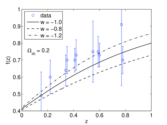
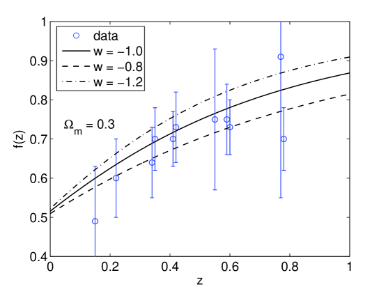
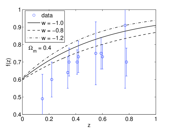
To get a sense of the dependence of the growth rate on different cosmological parameters, we plot the evolution behavior of as a function of redshift for different values of and in Fig. 1. We can see that the influence of on the growth rate is small at relatively low redshifts and becomes much larger at high redshifts. On the other hand, for the three values of considered in Fig. 1, the curve of deviate from each other. This is expected, as one can see from Eq. (7) that the contribution of comes from while mainly affects the index . The 11 observational data points are also shown in the figure. It can be seen that the error bars are quite large, which is still a serious problem for the current growth rate data. However, it can still be seen that the middle panel coincides with the data very well, suggesting that lies around 0.3, which is in agreement with other observational constraints. This preliminary result will be studied quantitatively in the next section.
4 SNIa, BAO and CMB data
As we have mentioned earlier, due to the large error bars of growth rate data, we need to integrate other data to obtain better constraints on the cosmological parameters. In this paper we use the SNIa, BAO and CMB data to place joint constraints on the dark energy models.
4.1 SNIa data
Currently, SN Ia is the most powerful tool to study the dark energy due to its reliability as standard candles. For the SNIa data, we use the latest UNION2 compilation [3] which, in total, contains 557 type Ia supernovae with redshifts ranging from 0.511 to 1.12. Since there are too many data points, we will not list them here. For details of the data, readers can refer to Amanullah et al. [3]. Cosmological constraints from the SNIa data are obtained through the distance modulus . The theoretical distance modulus is
| (12) |
where with being the Hubble constant in units of 100 km/s/Mpc, and the Hubble-free luminosity distance is defined as
| (13) |
where and is the present curvature density. Here the symbol sinn(x) stands for sinh(x) (), sin(x) () or just x ().
To compute the for the SNIa data, we follow [34] to analytically marginalize over the nuisance parameter ,
| (14) |
where
| (15) | ||||
Here is the uncertainty in the distance moduli. Eq. (14) has a minimum at where
| (16) |
This equation is independent of , so instead of we adopt to compute the likelihood.
4.2 BAO data
The competition between the gravitational force and the relativistic primordial plasma pressure gives rise to acoustic oscillations which leaves its signature in every epoch of the universe. Eisenstein et al. [22] first found a peak of this baryon acoustic oscillations in the large-scale correlation function at 100 Mpc separation from a spectroscopic sample of 46,748 luminous red galaxies of the Sloan Digital Sky Survey (SDSS). Percival et al. [38] performed a power-spectrum analysis of the SDSS DR7 dataset, considering both the main and LRG samples, and measured the BAO signal at both and . For low redshifts, the 6dF Galaxy Survey (6dFGS) group have reported a BAO detection at [5]. Most recently, Blake et al. [9] presented measurements of the BAO peak at redshifts and 0.73 in the galaxy correlation function of the final dataset of the WiggleZ Dark Energy Survey. They combined their WiggleZ BAO measurements with the SDSS DR7 and 6dFGS datasets to present tight constraints on the dark energy. In this work, We follow their methods to constrain different dark energy models by using their combined BAO datasets.
The data can be found in the above papers, but for completeness we summarize the BAO measurements from the three surveys and the way we use them.
The for the WiggleZ BAO data is given by [9],
| (17) |
where the data vector is for the effective redshift and 0.73. The corresponding theoretical value denotes the acoustic parameter introduced by [22]:
| (18) |
where the distance scale is defined as
| (19) |
Here is the Hubble-free angular diameter distance which relates to the Hubble-free luminosity distance through , and . The inverse covariance matrix is given by
| (20) |
Similarly, for the SDSS DR7 BAO distance measurements, the can be expressed as [38]
| (21) |
where is a vector containing the datapoints at and . denotes the theoretical distance ratio
| (22) |
Here, is the comoving sound horizon,
| (23) |
where the sound speed , with and = 2.726K.
in Eq. (21) is the inverse covariance matrix for the SDSS data set given by
| (26) |
For the 6dFGS BAO data [5], there is only one data point at , so the is easy to compute:
| (27) |
The total for all the BAO data sets can therefore be written as
| (28) |
For clarity, we have given all the BAO data sets used in our study in Table 2. The errors are contained in the inverse covariance matrixes presented in Eqs. (20) and (26).
4.3 CMB data
Since the SNIa and BAO data contain information about the universe at relatively low redshifts, we will include the CMB information by implementing the WMAP 7-year data [30] to probe the entire expansion history up to the last scattering surface. The for the CMB data is constructed as
| (29) |
where
| (30) |
Here is the “acoustic scale” defined as
| (31) |
where the redshift of decoupling is given by [27],
| (32) |
| (33) |
The “shift parameter” () in Eq. (30) is defined as [10]
| (34) |
and is the inverse covariance matrix
| (35) |
For completeness, we have also given the CMB data used in our study in Table 2. The errors are contained in the inverse covariance matrixes presented in Eq. (35).
5 Results
To show the function of the growth rate data, we first use these data alone to constrain the three dark energy models described in Section 2. We then combine the growth rate data with the SNIa, BAO and CMB data to get the joint results. We use the Markov Chain Monte Carlo (MCMC) method to search in the parameter spaces and determine the best-fit parameters. Our MCMC code is based on the publicly available CosmoMC package [31].
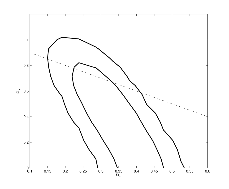
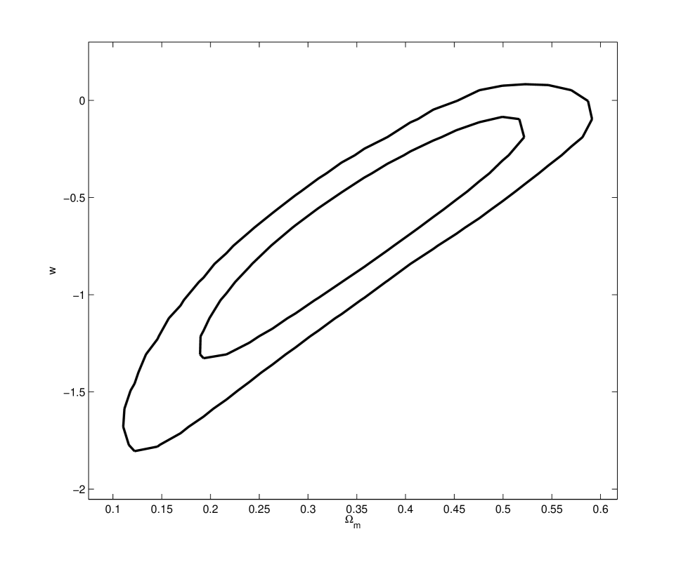
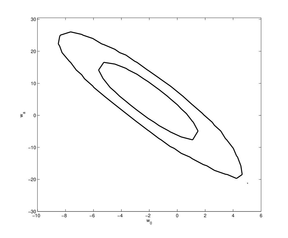
Figs. 24 show the constraints on the dark energy models from the growth rate data alone. It can be seen that the current growth rate data generally support the CDM model within the 1 confidence level. However, the contours are quite broad and are not as stringent as those from the SNIa or BAO + CMB data. Anyway, the results are comparable to those of the Hubble parameter data [16], the gamma-ray burst data [42], and the strong gravitational lensing data [14]. The best fit parameters are listed in Table 3. We notice that the growth rate data alone tend to favor a larger in the CDM and wCDM case. The constraints on and are not that stringent, mainly due to the sparsity and large error bars of current growth rate data. As for the CPL model, because of the large number of parameters, the constraints are much weaker. Despite the large error bars of current growth rate data, it can be seen that they still give reasonable results for the three dark energy models, and the concordance CDM model is still favored by these growth rate data.
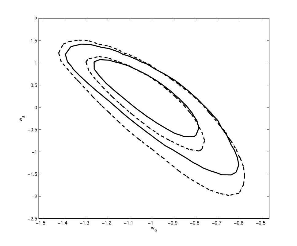
To get better constraints on the dark energy parameters and to see the influence on the results when adding the growth rate data to other data sets, we also perform a joint analysis combining the SNIa, BAO and CMB data. For this purpose, the total is defined as
| (36) |
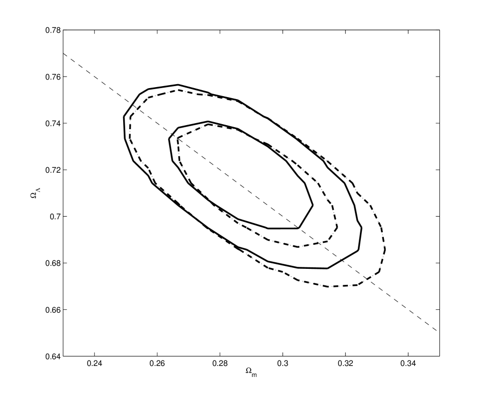
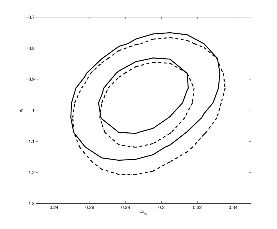
Figs. 57 show the constraints on the cosmological parameters with and without the growth rate data. It can be seen that adding the growth rate data to the combination of the SNIa, BAO and CMB data do affect the results. In all the three figures, including the growth rate data improves the joint constraints. This is most obvious in Fig. 5 and Fig. 7. In Fig. 6, the results are also improved slightly by adding the growth rate data. Meanwhile, the contours shift somewhat towards the high-w end, suggesting that the growth rate data prefer a larger , consistent with the earlier results we just obtained. Of course, currently these growth rate data are not able to compete with the three most powerful datasets – SNIa, CMB and BAO, but they can help strengthen the constraints on the dark energy, which is a good sign. Table 3 also presents the best-fit parameters of the three dark energy models using different combinations of the data sets. The results are consistent with those of Blake et al. [9], who have also tested the three dark energy models using the new SNIa, BAO and CMB data.
Generally speaking, the concordance CDM model is well consistent with currently available data. However, alternative models like the wCDM and CPL models cannot be excluded yet. Therefore, more observational data are required for a clear discrimination between these models. Anyway, our study shows that we can use the growth rate data as an important supplement to the SNIa, BAO and CMB data to probe the dark energy, as they can serve to strengthen the constraints. Currently these data are heavily restricted by the large errors. It is expected that future observations will provide more of these independent growth rate data along with higher accuracy, to help us place better constraints on the dark energy.
6 Conclusion and discussion
In this work, we have used the observational growth rate data to set constraints on three dark energy models. These growth rate data are mainly derived from redshift surveys using redshift distortions, including the latest WiggleZ dark energy survey data which are much more precise than previous data.
Because most of the data are obtained under the assumption of general relativity and the CDM model, we do not use them to constrain the modified gravity models as usually done in previous studies. To be conservative, we only use them to constrain the mildly time-evolving dark energy models which deviate not quite far from the CDM model. We expect that future redshift surveys would examine the AP effect more accurately, and thus could improve the usage of the growth rate data for constraining the cosmological parameters.
There is an important advantage in using these data to constrain the cosmological parameters. Unlike many other cosmological probes (e.g. the BAO, CMB and Observational Hubble parameter), the growth rate data are completely independent of the Hubble constant , thus they may help break the degeneracy between and other parameters. Due to the large error bars and the sparsity of the available data, the growth rate data alone currently cannot give quite stringent constraints on the model parameters. But they still support the concordance CDM model at the 1 confidence level, as shown in Figs. 24. Meanwhile, they seem to prefer larger values of and . Combined with other data sets, the growth rate data can improve the constraints, as can be seen in Figs. 57, where the contours become smaller after adding the growth rate data. Our joint analysises show that the CDM model is still in good agreement with current data, but a time-evolving dark energy can not be excluded yet. As an independent data set, the growth rate data can help tighten the constraints of the SNIa, BAO and CMB data. It is a good sign for using the growth rate data to constrain the cosmological parameters.
We anticipate that future redshift surveys will provide more reliable and accurate growth rate data. In conjunction with other observational data, the growth rate data should be quite helpful for us to understand the cosmic acceleration.
Acknowledgments
We thank the anonymous referee for helpful comments and suggestions. KS is very grateful to Luigi Guzzo for valuable discussions and suggestions. We also would like to thank Shi Qi and Bo Yu for useful discussions. This work was supported by the National Basic Research Program of China (973 program, Grant No. 2009CB824800), the National Natural Science Foundation of China (Grant Nos. 11033002 and 10973039).
| z | f(z) | Reference | |
|---|---|---|---|
| 0.15 | 0.49 | 0.14 | [25] |
| 0.22 | 0.60 | 0.10 | [7] |
| 0.34 | 0.64 | 0.09 | [11] |
| 0.35 | 0.70 | 0.08 | [47] |
| 0.41 | 0.70 | 0.07 | [7] |
| 0.42 | 0.73 | 0.09 | [8] |
| 0.55 | 0.75 | 0.18 | [41] |
| 0.59 | 0.75 | 0.09 | [8] |
| 0.60 | 0.73 | 0.07 | [7] |
| 0.77 | 0.91 | 0.36 | [25] |
| 0.78 | 0.70 | 0.08 | [7] |
| BAO | z | A(z) | Reference | |
| 6dFGS | 0.106 | 0.336 | [5] | |
| SDSS | 0.2 | 0.1905 | [38] | |
| SDSS | 0.35 | 0.1097 | [38] | |
| WiggleZ | 0.44 | 0.474 | [9] | |
| WiggleZ | 0.6 | 0.442 | [9] | |
| WiggleZ | 0.73 | 0.424 | [9] | |
| CMB | R | Reference | ||
| WMAP | 1091.3 | 302.09 | 1.725 | [30] |
| Model | growth rate | SNIa + BAO + CMB | SNIa + BAO + CMB + growth rate |
| CDM | = | = | = |
| wCDM | = | = | = |
| = | = | = | |
| CPL | = | = | = |
| = | = | ||
| = | = | = |
References
- Alcock & Paczynski [1979] Alcock, C. & Paczynski, B. 1979, Nature, 281, 358
- Allen et al. [2008] Allen, S. W., Rapetti, D. A., Schmidt, R. W., Ebeling, H., Morris, R. G., & Fabian, A. C. 2008, MNRAS, 383, 879
- Amanullah et al. [2010] Amanullah, R., Lidman, C., Rubin, D., Aldering, G., Astier, P., Barbary, K., Burns, M. S., Conley, A., Dawson, K. S., Deustua, S. E., Doi, M., Fabbro, S., Faccioli, L., Fakhouri, H. K., Folatelli, G., Fruchter, A. S., Furusawa, H., Garavini, G., Goldhaber, G., Goobar, A., Groom, D. E., Hook, I., Howell, D. A., Kashikawa, N., Kim, A. G., Knop, R. A., Kowalski, M., Linder, E., Meyers, J., Morokuma, T., Nobili, S., Nordin, J., Nugent, P. E., Östman, L., Pain, R., Panagia, N., Perlmutter, S., Raux, J., Ruiz-Lapuente, P., Spadafora, A. L., Strovink, M., Suzuki, N., Wang, L., Wood-Vasey, W. M., Yasuda, N., & Supernova Cosmology Project, T. 2010, ApJ, 716, 712
- Bertschinger [2006] Bertschinger, E. 2006, ApJ, 648, 797
- Beutler et al. [2011] Beutler, F., Blake, C., Colless, M., Jones, D. H., Staveley-Smith, L., Campbell, L., Parker, Q., Saunders, W., & Watson, F. 2011, MNRAS, 416, 3017
- Biesiada et al. [2010] Biesiada, M., Piórkowska, A., & Malec, B. 2010, MNRAS, 406, 1055
- Blake et al. [2011a] Blake, C., Brough, S., Colless, M., Contreras, C., Couch, W., Croom, S., Davis, T., Drinkwater, M. J., Forster, K., Gilbank, D., Gladders, M., Glazebrook, K., Jelliffe, B., Jurek, R. J., Li, I.-H., Madore, B., Martin, D. C., Pimbblet, K., Poole, G. B., Pracy, M., Sharp, R., Wisnioski, E., Woods, D., Wyder, T. K., & Yee, H. K. C. 2011a, MNRAS, 834
- Blake et al. [2010] Blake, C., Brough, S., Colless, M., Couch, W., Croom, S., Davis, T., Drinkwater, M. J., Forster, K., Glazebrook, K., Jelliffe, B., Jurek, R. J., Li, I.-H., Madore, B., Martin, C., Pimbblet, K., Poole, G. B., Pracy, M., Sharp, R., Wisnioski, E., Woods, D., & Wyder, T. 2010, MNRAS, 406, 803
- Blake et al. [2011b] Blake, C., Kazin, E. A., Beutler, F., Davis, T. M., Parkinson, D., Brough, S., Colless, M., Contreras, C., Couch, W., Croom, S., Croton, D., Drinkwater, M. J., Forster, K., Gilbank, D., Gladders, M., Glazebrook, K., Jelliffe, B., Jurek, R. J., Li, I.-H., Madore, B., Martin, D. C., Pimbblet, K., Poole, G. B., Pracy, M., Sharp, R., Wisnioski, E., Woods, D., Wyder, T. K., & Yee, H. K. C. 2011b, MNRAS, 1598
- Bond et al. [1997] Bond, J. R., Efstathiou, G., & Tegmark, M. 1997, MNRAS, 291, L33
- Cabré & Gaztañaga [2009] Cabré, A. & Gaztañaga, E. 2009, MNRAS, 393, 1183
- Caldwell [2002] Caldwell, R. R. 2002, Phys. Lett. B, 545, 23
- Caldwell et al. [1998] Caldwell, R. R., Dave, R., & Steinhardt, P. J. 1998, Phys. Rev. Lett., 80, 1582
- Cao et al. [2011] Cao, S., Pan, Y., Biesiada, M., Godlowski, W., & Zhu, Z.-H. 2011, ArXiv:1105.6226
- Capozziello et al. [2004] Capozziello, S., Cardone, V. F., Funaro, M., & Andreon, S. 2004, Phys. Rev. D, 70, 123501
- Chen & Ratra [2011] Chen, Y. & Ratra, B. 2011, ArXiv:1106.4294
- Chevallier & Polarski [2001] Chevallier, M. & Polarski, D. 2001, Int. J. Modern Phys. D, 10, 213
- Copeland et al. [2006] Copeland, E. J., Sami, M., & Tsujikawa, S. 2006, Int. J. Modern Phys. D, 15, 1753
- Courtin et al. [2011] Courtin, J., Rasera, Y., Alimi, J.-M., Corasaniti, P.-S., Boucher, V., & Füzfa, A. 2011, MNRAS, 410, 1911
- di Porto & Amendola [2008] di Porto, C. & Amendola, L. 2008, Phys. Rev. D, 77, 083508
- Eisenstein & Hu [1998] Eisenstein, D. J. & Hu, W. 1998, ApJ, 496, 605
- Eisenstein et al. [2005] Eisenstein, D. J., Zehavi, I., Hogg, D. W., Scoccimarro, R., Blanton, M. R., Nichol, R. C., Scranton, R., Seo, H.-J., Tegmark, M., Zheng, Z., Anderson, S. F., Annis, J., Bahcall, N., Brinkmann, J., Burles, S., Castander, F. J., Connolly, A., Csabai, I., Doi, M., Fukugita, M., Frieman, J. A., Glazebrook, K., Gunn, J. E., Hendry, J. S., Hennessy, G., Ivezić, Z., Kent, S., Knapp, G. R., Lin, H., Loh, Y.-S., Lupton, R. H., Margon, B., McKay, T. A., Meiksin, A., Munn, J. A., Pope, A., Richmond, M. W., Schlegel, D., Schneider, D. P., Shimasaku, K., Stoughton, C., Strauss, M. A., SubbaRao, M., Szalay, A. S., Szapudi, I., Tucker, D. L., Yanny, B., & York, D. G. 2005, ApJ, 633, 560
- Fu et al. [2008] Fu, L., Semboloni, E., Hoekstra, H., Kilbinger, M., van Waerbeke, L., Tereno, I., Mellier, Y., Heymans, C., Coupon, J., Benabed, K., Benjamin, J., Bertin, E., Doré, O., Hudson, M. J., Ilbert, O., Maoli, R., Marmo, C., McCracken, H. J., & Ménard, B. 2008, A&A, 479, 9
- Gironés et al. [2010] Gironés, Z., Marchetti, A., Mena, O., Peña-Garay, C., & Rius, N. 2010, J. Cosmology Astropart. Phys., 11, 4
- Guzzo et al. [2008] Guzzo, L., Pierleoni, M., Meneux, B., Branchini, E., Le Fèvre, O., Marinoni, C., Garilli, B., Blaizot, J., De Lucia, G., Pollo, A., McCracken, H. J., Bottini, D., Le Brun, V., Maccagni, D., Picat, J. P., Scaramella, R., Scodeggio, M., Tresse, L., Vettolani, G., Zanichelli, A., Adami, C., Arnouts, S., Bardelli, S., Bolzonella, M., Bongiorno, A., Cappi, A., Charlot, S., Ciliegi, P., Contini, T., Cucciati, O., de la Torre, S., Dolag, K., Foucaud, S., Franzetti, P., Gavignaud, I., Ilbert, O., Iovino, A., Lamareille, F., Marano, B., Mazure, A., Memeo, P., Merighi, R., Moscardini, L., Paltani, S., Pellò, R., Perez-Montero, E., Pozzetti, L., Radovich, M., Vergani, D., Zamorani, G., & Zucca, E. 2008, Nature, 451, 541
- Hirano et al. [2011] Hirano, K., Komiya, Z., & Shirai, H. 2011, ArXiv:1103.6133
- Hu & Sugiyama [1996] Hu, W. & Sugiyama, N. 1996, ApJ, 471, 542
- Johri & Rath [2007] Johri, V. B. & Rath, P. K. 2007, Int. J. Modern Phys. D, 16, 1581
- Kaiser [1987] Kaiser, N. 1987, MNRAS, 227, 1
- Komatsu et al. [2011] Komatsu, E., Smith, K. M., Dunkley, J., Bennett, C. L., Gold, B., Hinshaw, G., Jarosik, N., Larson, D., Nolta, M. R., Page, L., Spergel, D. N., Halpern, M., Hill, R. S., Kogut, A., Limon, M., Meyer, S. S., Odegard, N., Tucker, G. S., Weiland, J. L., Wollack, E., & Wright, E. L. 2011, ApJS, 192, 18
- Lewis & Bridle [2002] Lewis, A. & Bridle, S. 2002, Phys. Rev. D, 66, 103511
- Linder [2003] Linder, E. V. 2003, Phys. Rev. Lett., 90, 091301
- Linder [2005] —. 2005, Phys. Rev. D, 72, 043529
- Nesseris & Perivolaropoulos [2005] Nesseris, S. & Perivolaropoulos, L. 2005, Phys. Rev. D, 72, 123519
- Nesseris & Perivolaropoulos [2008] —. 2008, Phys. Rev. D, 77, 023504
- Peebles & Ratra [2003] Peebles, P. J. & Ratra, B. 2003, Rev. Mod. Phys., 75, 559
- Peebles [1980] Peebles, P. J. E. 1980, The large-scale structure of the universe, ed. Peebles, P. J. E.
- Percival et al. [2010] Percival, W. J., Reid, B. A., Eisenstein, D. J., Bahcall, N. A., Budavari, T., Frieman, J. A., Fukugita, M., Gunn, J. E., Ivezić, Ž., Knapp, G. R., Kron, R. G., Loveday, J., Lupton, R. H., McKay, T. A., Meiksin, A., Nichol, R. C., Pope, A. C., Schlegel, D. J., Schneider, D. P., Spergel, D. N., Stoughton, C., Strauss, M. A., Szalay, A. S., Tegmark, M., Vogeley, M. S., Weinberg, D. H., York, D. G., & Zehavi, I. 2010, MNRAS, 401, 2148
- Perlmutter et al. [1999] Perlmutter, S., Aldering, G., Goldhaber, G., Knop, R. A., Nugent, P., Castro, P. G., Deustua, S., Fabbro, S., Goobar, A., Groom, D. E., Hook, I. M., Kim, A. G., Kim, M. Y., Lee, J. C., Nunes, N. J., Pain, R., Pennypacker, C. R., Quimby, R., Lidman, C., Ellis, R. S., Irwin, M., McMahon, R. G., Ruiz-Lapuente, P., Walton, N., Schaefer, B., Boyle, B. J., Filippenko, A. V., Matheson, T., Fruchter, A. S., Panagia, N., Newberg, H. J. M., Couch, W. J., & The Supernova Cosmology Project. 1999, ApJ, 517, 565
- Riess et al. [1998] Riess, A. G., Filippenko, A. V., Challis, P., Clocchiatti, A., Diercks, A., Garnavich, P. M., Gilliland, R. L., Hogan, C. J., Jha, S., Kirshner, R. P., Leibundgut, B., Phillips, M. M., Reiss, D., Schmidt, B. P., Schommer, R. A., Smith, R. C., Spyromilio, J., Stubbs, C., Suntzeff, N. B., & Tonry, J. 1998, AJ, 116, 1009
- Ross et al. [2007] Ross, N. P., da Ângela, J., Shanks, T., Wake, D. A., Cannon, R. D., Edge, A. C., Nichol, R. C., Outram, P. J., Colless, M., Couch, W. J., Croom, S. M., de Propris, R., Drinkwater, M. J., Eisenstein, D. J., Loveday, J., Pimbblet, K. A., Roseboom, I. G., Schneider, D. P., Sharp, R. G., & Weilbacher, P. M. 2007, MNRAS, 381, 573
- Samushia & Ratra [2010] Samushia, L. & Ratra, B. 2010, ApJ, 714, 1347
- Schaefer [2007] Schaefer, B. E. 2007, ApJ, 660, 16
- Spergel et al. [2003] Spergel, D. N., Verde, L., Peiris, H. V., Komatsu, E., Nolta, M. R., Bennett, C. L., Halpern, M., Hinshaw, G., Jarosik, N., Kogut, A., Limon, M., Meyer, S. S., Page, L., Tucker, G. S., Weiland, J. L., Wollack, E., & Wright, E. L. 2003, ApJS, 148, 175
- Stern et al. [2010] Stern, D., Jimenez, R., Verde, L., Kamionkowski, M., & Stanford, S. A. 2010, J. Cosmology Astropart. Phys., 2, 8
- Sullivan et al. [2011] Sullivan, M., Guy, J., Conley, A., Regnault, N., Astier, P., Balland, C., Basa, S., Carlberg, R. G., Fouchez, D., Hardin, D., Hook, I. M., Howell, D. A., Pain, R., Palanque-Delabrouille, N., Perrett, K. M., Pritchet, C. J., Rich, J., Ruhlmann-Kleider, V., Balam, D., Baumont, S., Ellis, R. S., Fabbro, S., Fakhouri, H. K., Fourmanoit, N., Gonzalez-Gaitan, S., Graham, M. L., Hudson, M. J., Hsiao, E., Kronborg, T., Lidmam, C., Mourao, A. M., Neill, J. D., Perlmutter, S., Ripoche, P., Suzuki, N., & Walker, E. S. 2011, ArXiv:1104.1444
- Tegmark et al. [2006] Tegmark, M., Eisenstein, D. J., Strauss, M. A., Weinberg, D. H., Blanton, M. R., Frieman, J. A., Fukugita, M., Gunn, J. E., Hamilton, A. J. S., Knapp, G. R., Nichol, R. C., Ostriker, J. P., Padmanabhan, N., Percival, W. J., Schlegel, D. J., Schneider, D. P., Scoccimarro, R., Seljak, U., Seo, H.-J., Swanson, M., Szalay, A. S., Vogeley, M. S., Yoo, J., Zehavi, I., Abazajian, K., Anderson, S. F., Annis, J., Bahcall, N. A., Bassett, B., Berlind, A., Brinkmann, J., Budavari, T., Castander, F., Connolly, A., Csabai, I., Doi, M., Finkbeiner, D. P., Gillespie, B., Glazebrook, K., Hennessy, G. S., Hogg, D. W., Ivezić, Ž., Jain, B., Johnston, D., Kent, S., Lamb, D. Q., Lee, B. C., Lin, H., Loveday, J., Lupton, R. H., Munn, J. A., Pan, K., Park, C., Peoples, J., Pier, J. R., Pope, A., Richmond, M., Rockosi, C., Scranton, R., Sheth, R. K., Stebbins, A., Stoughton, C., Szapudi, I., Tucker, D. L., vanden Berk, D. E., Yanny, B., & York, D. G. 2006, Phys. Rev. D, 74, 123507
- Weinberg [1989] Weinberg, S. 1989, Rev. Mod. Phys., 61, 1
- Xia [2009] Xia, J.-Q. 2009, Phys. Rev. D, 79, 103527
- Zlatev et al. [1999] Zlatev, I., Wang, L., & Steinhardt, P. J. 1999, Phys. Rev. Lett., 82, 896