Critical network effect induces business oscillations in multi-level marketing systems

Abstract

Business-cycle phenomenon has long been regarded as an empirical curiosity in macroeconomics. Regarding its causes, recent evidence suggests that economic oscillations are engendered by fluctuations in the level of entrepreneurial activitybeamish2010 ; koellinger2011 . Opportunities promoting such activity are known to be embedded in social network structureseagle2010 ; granovetter2005 . However, predominant understanding of the dynamics of economic oscillations originates from stylised pendulum models on aggregate macroeconomic variablesminsky1957 ; sims1980 , which overlook the role of social networks to economic activity—echoing the so-called aggregation problem of reconciling macroeconomics with microeconomicscolander2008 ; elsner2007 . Here I demonstrate how oscillations can arise in a networked economy epitomised by an industry known as multi-level marketing or MLMalbaum2011 , the lifeblood of which is the profit-driven interactions among entrepreneurs. Quarterly data (over a decade) which I gathered from public MLMs reveal oscillatory time-series of entrepreneurial activity that display nontrivial scaling and persistencemorales2012 ; dimatteo2007 . I found through a stochastic population-dynamic model, which agrees with the notion of profit maximisation as the organising principle of capitalist enterprise, that oscillations exhibiting those characteristics arise at the brink of a critical balance between entrepreneurial activation and inactivation brought about by a homophily-driven network effect. Oscillations develop because of stochastic tunnelling permitted through the destabilisation by noise of an evolutionarily stable state. The results fit altogether as evidence to the Burns-Mitchell conjecture that economic oscillations must be induced by the workings of an underlying “network of free enterprises searching for profit”burns1954 . I anticipate that the findings, interpreted under a mesoeconomic frameworkdopfer2012 , could open a viable window for scrutinising the nature of business oscillations through the lens of the emerging field of network science. Enquiry along these lines could shed further light into the network origins of the business-cycle phenomenon.

Known widely in literature as network marketing, MLM executes through embedded social networks its essential business functions such as goods distribution, consumption, marketing, and direct sellingalbaum2011 ; coughlan1998 . That makes MLM a stark microcosm of a networked economy. One salient yet so far overlooked feature of MLM dynamics is the aperiodic oscillations in firm size $N(t)$, quantified by the number of participating entrepreneurs (Fig. 1). Empirical quarterly firm-size data have been collected from four public MLMs (Supplementary Data; Supplementary Methods, S1): NuSkin Enterprises (NUS), Nature Sunshine (NATR), USANA Health Sciences (USNA), and Mannatech Inc. (MTEX). Publicly-listed firms are chosen because they are required to disclose accurate business data on a regular basis. The average revenue (i.e., total revenue divided by $N$ for any given quarter) does not proportionately rise with $N$ (Fig. 1c,d), implying that firm-size expansion does not inevitably translate into revenue growth. Firm size is thus a more reliable quantifier for entrepreneurial activity than is total revenue.

The scaling property of the $N(t)$ time-series is examined via Hurst analysismorales2012 ; dimatteo2007 (Methods; Supplementary Methods, S1). The Hurst exponents, $H(1)$ and $H(2)$, quantify the scaling of the absolute increments and of the power spectrum, respectively. If time series were generated by a Wiener process, such as in the Black-Scholes modelborland2002 , then $H(1)=0.5$. But $H(1)>0.5$ indicates persistence, i.e., changes in one direction usually occur in consecutive periods; whereas $H(1)<0.5$ suggests anti-persistence, i.e., changes in opposite directions usually appear in sequencedimatteo2007 . Ideally, a single scaling regime means $H(1)=H(2)$, which applies to time-series generated by unifractal processes such as the Wiener process and the fractal Brownian motion. Table 1 presents Hurst exponents for different MLMs. Generally, $H(1)>0.5$ except for NUS North Asia and NATR with $H(1)\sim 0.5$ (within standard deviation); and $H(1)=H(2)$ within standard deviation. Overall, these features of the time-series suggest that MLM firm dynamics is a non-Wiener unifractal processdimatteo2007 . Unifractality implies self-similarity such that conclusions drawn at one timescale remains statistically valid at another timescale.

Table 1: Hurst exponents $H(1)$ and $H(2)$ for different MLMs estimated using the generalised Hurst methoddimatteo2007 ; morales2012 . $H(1)>0.5$ indicates persistence, whereas $H(1)<0.5$ indicates anti-persistence. $H(2)$ values, which are closely related to the scaling of the power spectrum, are also shown. Generally, $H(2)=H(1)$ within standard deviation. The standard deviation values are determined from a pre-testing procedure (Supplementary Methods, S1).

$MLM$	$H(1)$	$H(2)$
MTEX	$0.8328\pm 0.1140$	$0.7425\pm 0.1081$
USNA United States	$0.7602\pm 0.1140$	$0.6823\pm 0.1081$
USNA Canada	$0.6619\pm 0.1140$	$0.6013\pm 0.1081$
USNA SEA-Pacific	$0.6383\pm 0.1140$	$0.6139\pm 0.1081$
NUS Greater China	$0.6159\pm 0.1098$	$0.5387\pm 0.1038$
NATR	$0.5128\pm 0.1032$	$0.5126\pm 0.0876$
NUS North Asia	$0.4780\pm 0.1098$	$0.4789\pm 0.1038$

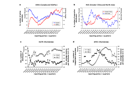
Figure 1: Empirical data for different publicly-listed MLM firms. $N(t)$ is the firm size, $R(t)$ is average revenue per member, and $t$ is time in quarters. a, USANA Health Sciences (USNA) in Canada, and Southeast Asia and Pacific (including Australia) from March 1998 to March 2012. b, NuSkin (NUS) in Greater China (including Hong Kong) and North Asia (Japan and South Korea) from March 1999 to March 2012. c, Nature Sunshine (NATR) worldwide showing $N$ and $R$ from September 1994 to March 2012. d, Mannatech Inc. (MTEX) worldwide showing $N$ and $R$ from April 1998 to March 2012. Data sets are provided in Supplementary Data.

An MLM firm is considered as a population of profit-seeking entrepreneurs. This population exhibits disorder through the presence of two entrepreneur types distinguished by socio-economic status (SES). Let $A$ and $B$ denote these types, wherein $A$ has higher SES than $B$, and $N_{A}$ and $N_{B}$ denote their subpopulation size, respectively. The total population at any given time $t$ is thus $N(t)=N=N_{A}+N_{B}$. Three major processes run the population dynamics: entrepreneurial activation by recruitment; competitive inactivation; and catalytic inactivation due to a network effect. Recruitment is expressed in the following reaction equations:

$$A\overset{\mu}{\longrightarrow}2A, \quad B\overset{\mu}{\longrightarrow}B+A,$$

$$B\overset{\lambda}{\longrightarrow}2B, \quad A\overset{\lambda}{\longrightarrow}A+B,$$ (1)

wherein $\mu$ and $\lambda$ are per-capita rates of recruitment of types $A$ and $B$, respectively, and $\mu>\lambda$ because $A$’s higher SES implies a faster rate of entrepreneurial activation through the support of bigger capital and vaster social resources. Competitive inactivation occurs due to market overlap, or niche overlapgimeno2004 , as participants can go head-to-head over the same clientele or market. An encounter rate $\delta$, which can be related to the density of the embedding social network, quantifies the probability of market overlaps. Thus, competitive inactivation is:

$$Z+A\overset{\delta}{\longrightarrow}Z,\quad Z+B\overset{\delta}{\longrightarrow}Z\quad\mathrm{for}\;Z\in\left\{A,B\right\}.$$ (2)

Lastly, catalytic inactivation, which denotes the network effect (Methods), is expressed as:

$$Z\underset{{\mathbf{MLM}}}{\overset{{\nu\Phi}}{\xrightarrow{\hskip 28.45274pt}}}\varnothing,\quad\mathrm{for}\;Z\in\left\{A,B\right\}.$$ (3)

The network structure of the MLM catalyses inactivation of existing participants at the rate $\nu\,\Phi$, where $\Phi=\dfrac{\sum_{Z\in\{A,B\}}N_{Z}\left(N_{Z}-1\right)}{N(N-1)}$ is a measure of the probability that two members drawn randomly from the MLM belong to the same type. It has been widely used in literature as a diversity indexsimpson1949 . Due to interconnectedness and homophilyapicella2012 , the inactivation of one could (like a contagion) infect another to follow suit.

Combining equations (1– 3) results to a Master equation (Supplementary Equation 1) for the state probability density. Perturbation analysis accounts for the fluctuations arising from demographic stochasticityvankampen2007 . In terms of the system size $\Omega$ (roughly the size of that part of the overall population considered fit for entrepreneurial activities) the following ansatz is made: $N_{A}=\Omega\alpha+\sqrt{\Omega}\,a$ and $N_{B}=\Omega\beta+\sqrt{\Omega}\,b$, where $\alpha$ and $\beta$ are the average concentrations, and $a$ and $b$ are the magnitude of the fluctuations of the stochastic variables $N_{A}$ and $N_{B}$, respectively (Supplementary Methods, S2). The highest order in the expansion expresses the macroscopic rate equations for $\alpha$ and $\beta$:

$$\dot{\alpha} =\mu(\alpha+\beta)-\nu\,\Phi\,(\alpha+\beta)-\delta\,(\alpha+\beta)\alpha;$$

$$\dot{\beta} =\lambda(\alpha+\beta)-\nu\,\Phi\,(\alpha+\beta)-\delta\,(\alpha+\beta)\beta.$$ (4)

Meanwhile, the next highest order term gives the Fokker-Planck equation, or FPE (Supplementary Equation 2), governing the dynamics of the probability density for the magnitude of the fluctuations. From the FPE, the expectation values of the stationary fluctuations are $\left\langle a\right\rangle=\left\langle b\right\rangle=0$, which supports the interpretation that the deterministic solutions to (4) are the correct average values.

The model is nondimensionalised by setting the characteristic timescale at $t_{c}=5$ days (Methods). Consequently, the rates can be squarely related to empirical data by rescaling to appropriate units. Dimensionless rates take on simplified yet meaningful values: $\lambda=1-\mu$; $\mu,\nu\in(0,1)$; and $\Delta=\dfrac{ut_{c}\delta}{\Omega}\in\left(10^{-4},10^{-3}\right)$. Bifurcation analysis (Supplementary Methods, S4) of the nondimensionalised equation (4) unveils a bifurcation manifold $\mu=\mu_{b}(\nu)$, where

$$\mu_{b}(\nu)=\dfrac{1}{2}+\sqrt{\dfrac{\left(1-\nu\right)^{3}}{27\nu}},\quad 0<\nu<1.$$ (5)

Equation (5) coincides with an evolutionarily stable state (ESS) of a population game between the types (Supplementary Methods, S3– S4). The fraction of $A$– entrepreneurs is $x_{A}=\overline{x}_{A}+\Omega^{-1/2}\,\xi$, where $\overline{x}_{A}=\dfrac{\alpha}{\alpha+\beta}$, and $\xi$ is the fluctuation component. Analysis of the second moments from the FPE shows that the variance diverges as $\left\langle\xi^{2}\right\rangle\sim\delta\left|\mu-\mu_{b}\right|^{-1}$ as $\mu\rightarrow\mu_{b}^{-}$ (Supplementary Methods, S5). That is a signature of criticality through which the ESS, where $\overline{x}_{A}=x^{*}$ and $N=N^{*}=\dfrac{1-2\nu\,\Phi(x^{*})}{\Delta}$, is (quite counterintuitively) destabilised as the bifurcation manifold is approached. This mechanism is hereby referred as stochastic tunnelling wherein noise enables the state trajectory to cross a phase barrier that could not have been otherwise traversed without actively tuning the bifurcation parameter (Supplementary Methods, S4).

Stochastic tunnelling drives the business oscillations (Fig. 2). Time series is generated by solving the model using a numerical technique, known as Gillespie’s stochastic simulation algorithmgillespie1976 , which directly integrates the master equation (Supplementary Methods, S6). Diverging variance indeed allows the solution to wander far enough from the ESS and closer to an unstable point (UEP) which pushes that solution toward the boundary state, where $x^{*}=1$ and $N^{*}=\dfrac{\mu-\nu\Phi}{\Delta}$ (Fig. 2a). That noise also enables the solution to sling back to the ESS consequently forming loops in the phase portrait, hence, oscillations in the time series (Fig. 2b). The time series consist of upswings associated with increasing diversity and downswings with decreasing diversity, i.e., $\Phi\rightarrow 1$ as $x_{A}\rightarrow 1$. The remarkable observation is that recovery from low points of the series coincide with periods when $A$ is dominant—a case of the fitter entrepreneurs surviving through “recessions”blume2002 .

Profit maximisation is an axiom of capitalist enterpriseblume2002 . MLM may enhance profitability by maximising the proportion of $A$ – entrepreneurs (Supplementary Methods, S7). Thus, the time-average value $\left\langle x_{A}\right\rangle_{t}$ is examined for various pairs of $\mu$ and $\nu$ which consequently depicts the phase diagram of the model (Fig. 3a). Business oscillations come about as a result of stochastic tunnelling through the critical boundary $\mu=\mu_{b}$. Phase II, where $A$ stably dominates (Supplementary Fig. S2b), can be considered Pareto-optimal as the MLM maximises profitability as a whole. But high levels of targeted recruitment, i.e., $\mu>\dfrac{4}{7}$, are required. Entrepreneurial activation, however, might in reality be less discriminatory and thus $\mu\approx\dfrac{1}{2}$, which denotes higher entropy (Supplementary Discussion). The critical boundary delineates, for any magnitude $\nu$ of the network effect, the minimum $\mu$ that promotes long-run dominance of $A$ – entrepreneurs. Nevertheless, a stronger network effect tends to frustrate that dominance as catalytic inactivation increasingly outpaces activation, leading to degradation of entrepreneurial activity (Supplementary Fig. S2d). The ESS at the III-IV boundary (Fig. 3a) is therefore Pareto-dominated webb2007 .

The Hurst maps (Fig. 3b, c) locate where the real MLMs are on the phase diagram. The Hurst exponents are determined from the same exact method. Clusters appear in the vicinity of the III-IV boundary. On these clusters $H(1)$ and $H(2)$ are approximately between $0.5$ and $0.8$, about the same range of values found in real MLMs (see Table 1). A correlative plot (Fig. 3d) between $H(1)$ and $H(2)$ further confirms not only agreement between model and empirical data, but also their unifractality. Overall, these findings suggest that real-world MLMs are Pareto-dominated economic systemselsner2007 , which are operating in an environment characterised by high entropy, i.e., $\mu\approx\dfrac{1}{2}$, and by a strong network effect (i.e., $\nu>\mu$).

The study paints an illuminating insight about the nature of MLM operations. MLMs have been accused in several instances by discontent participants for ethical violations concerning its business practiceskoehn2001 . The model justifies such disgruntlement for two reasons. First, that profit is closely associated with recruitment implies less selective entrepreneurial activation. Second, that recruitment proceeds through embedded networks connotes strong network effects. Less-fit entrepreneurs can join the market in droves but are weeded out too soonblume2002 because of the Pareto-dominated nature of the venture. The feeling of being victimised is thus not at all surprising.

The mesoeconomic framework (i.e., linking microeconomic foundations with macroeconomic phenomenadopfer2012 ) puts the present study in a broader economic context. A more network-dynamic approach to viewing business cycles is hereby encouraged. Lastly, the mathematical model could be extended or refined, such as by generalising the network effect using the Hölder mean such that $\Phi(x_{A},x_{B})=\sqrt[q-1]{x_{A}^{q}+x_{B}^{q}},\;\forall q>1$ (Supplementary Discussion, Supplementary Fig. S1); whereas empirical data of higher temporal resolution may become available in the future, to further test the implications that came forth.

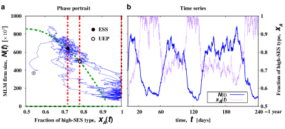
Figure 2: Business oscillations in the MLM. The model is simulated with the following parameters: $\mu=0.57$, $\nu=0.57$, $\Delta=5\times 10^{-4}$ for a total time of $t=240$ $1-$day periods $\approx 1$ year. a, Phase portrait showing one stochastic realization for $N(t)$ (in units $u=10^{3}$) versus $x_{A}(t)$; $\otimes$ marks the initial condition: $N(0)=400$ and $x_{A}(0)=0.54$. The dashed curves and lines are the nullclines of the replicator equations from the evolutionary game (Supplementary Methods, S3), which intersect at the evolutionarily stable state (ESS, $\bullet$) and at an unstable equilibrium point (UEP, $\circ$). The trajectory of the solution forms a loop indicating the oscillations. b, Time series for $N(t)$ and $x_{A}(t)$. Hurst analysis gives $H(1)=0.6668\pm 0.0235$ and $H(2)=0.6564\pm 0.0204$ for the $N(t)$ series.

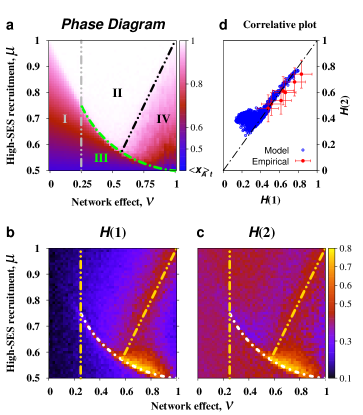
Figure 3: Phase diagram and Hurst maps of the MLM. a, $\left\langle x_{A}\right\rangle_{t}$ for different pairs of $\mu$ and $\nu$ (Resolution: $\Delta\mu\times\Delta\nu=0.01\times 0.02$). Phase I represents the regime $0\leq\nu\leq\dfrac{1}{4}$ where the critical manifold $\mu=\mu_{b}(\nu)$ is inaccessible due to the constraint $x_{A}\leq 1$. Phase II denotes the Pareto-optimal region $\mu>\mu_{b}(\nu)$ and $\mu>\nu$ where $x_{A}\approx 1$. Phase III, where $\mu<\mu_{b}$ is similar to phase I except that here the critical manifold is accessible. Phase IV is where $\mu>\mu_{b}$ but $\mu<\nu$ resulting to degradation of $N$ due to $\mu-\nu\,\Phi<0$ (Supplementary Fig. 2d). Phase boundaries: I–II,III, $\nu=\dfrac{1}{4}$; III—II,IV, $\mu=\mu_{b}(\nu)$; and II–IV, $\mu=\nu$. b, c, Map of the Hurst exponents $H(1)$ and $H(2)$, respectively. The phase boundaries are superimposed. The data are generated by simulating the model for $t=420$ $5-$day periods $\approx 8.75$ years with initial population $N(0)=100$ for different pairs of $\mu$ and $\nu$ (Resolution: $\Delta\mu\times\Delta\nu=0.01\times 0.02$). Each data pixel is an average of four stochastic realisations. d, Correlative plot between $H(1)$ and $H(2)$. Empirical data are those listed in Table 1. The dashed line $H(1)=H(2)$ denotes unifractality of the time series.

Methods

.1 Network effect.

The local network effect, which is a relatively new idea in economicssundararajan2008 ; galeotti2010 ; jackson2007 ; goeree2010 , means that the decision of one entity can influence those by whom that entity is connected to. Particularly, the network effect manifests through inactivation as the value of exiting the enterprise is enhanced through the catalytic action of the connections between participants. Homophilygoeree2010 ; apicella2012 spells that “a contact between similar people occurs at a higher rate than among dissimilar people”mcpherson2001 , and strongly influences contagions that diffuse through social linksaral2009 . MLM participants are thus more likely to connect with others of the same SES, consequently elevating homogeneity (or depressing diversity) in the firm. Diversity here is measured by the Simpson index $\Phi$ serving as a dimensionless potential function minimised when $N_{A}=N_{B}$ (at highest diversity). The network effect is constituted as $\nu\,\Phi$, for $\nu>0$; hence, the network effect is stronger at less diversity.

.2 Hurst analysis.

The generalized Hurst methodmorales2012 ; dimatteo2007 has been coded by one of its authors, T. Aste. The code was downloaded from Matlab File Exchange website, http://www.mathworks.com/matlabcentral/fileexchange/30076, and was used with default settings in the calculation of $H(1)$ and $H(2)$.

.3 Nondimensionalisation.

Dimensionless time is defined as $\widehat{t}=t/t_{c}$, wherein $t_{c}=\left(\mu+\lambda\right)^{-1}$. Population numbers are in units of $u$: $N_{A}=\widehat{N_{A}}\,u$ and $N_{B}=\widehat{N_{B}}\,u$. Consequently, equation (4) becomes:

$$\dfrac{d\widehat{N_{A}}}{d\widehat{t}} =\left(\mu t_{c}\right)\widehat{N_{A}}-\left(\nu t_{c}\right)\Phi(\widehat{N_{A}},\widehat{N_{B}})\,\left(\widehat{N_{A}}+\widehat{N_{B}}\right)-\left(ut_{c}\,\delta/\Omega\right)\left(\widehat{N_{A}}+\widehat{N_{B}}\right)\widehat{N_{A}},$$

$$\dfrac{d\widehat{N_{B}}}{d\widehat{t}} =\left(\lambda t_{c}\right)\widehat{N_{B}}-\left(\nu t_{c}\right)\Phi(\widehat{N_{A}},\widehat{N_{B}})\,\left(\widehat{N_{A}}+\widehat{N_{B}}\right)-\left(ut_{c}\,\delta/\Omega\right)\left(\widehat{N_{A}}+\widehat{N_{B}}\right)\widehat{N_{B}}.$$

Characteristic timescale is chosen at $t_{c}=5$ days (i.e., $1$ month $\equiv$ $20$ days). Assuming that the system-size parameter is of the order, $\Omega\sim 10^{6}$ individuals, and the unit $u\sim 10^{3}$ individuals, then setting $10^{-4}<\Delta=\dfrac{u\,t_{c}\,\delta}{\Omega}<10^{-3}$ implies an average per-capita encounter rate $\delta$ between $1$ and $10$ per month, which is a reasonable estimate.

References

- (1) Beamish, T. D. & Biggart N. W. Mesoeconomics: business cycles, entrepreneurship, and economic crisis in commercial building markets. In Lounsbury, M & Hirsch, P. M. (ed.), Markets on Trial: The Economic Sociology of the U.S. Financial Crisis: Part B Res. Soc. Org. 30, 245-280 (2010).
- (2) Koellinger, P. D. & Thurik, A. R. Entrepreneurship and the business cycle. Rev. Econ. Stat., doi:10.1162/REST_a_00224 (2011).
- (3) Eagle, N., Macy, M. & Claxton, R. Network diversity and economic development. Science 328, 1029-1031 (2010).
- (4) Granovetter, M. The impact of social structure on economic outcomes. J. Econ. Perspect. 19, 33-50 (2005).
- (5) Minsky, H. P. Monetary systems and accelerator models. Am. Econ. Rev. 47, 860-883 (1957).
- (6) Sims, C. A. Macroeconomics and reality. Econometrica 48, 1-48 (1980).
- (7) Colander, D., Howitt, P., Kirman, A., Leijonhufvud, A. & Mehrling, P. Beyond DSGE models: toward an empirically based macroeconomics. Am. Econ. Rev. Papers & Proc. 98, 236-240 (2008).
- (8) Elsner, W. Why meso? On “aggregation” and “emergence”, and why and how the meso level is essential in social economics. For. Soc. Econ. 36, 1-16 (2007).
- (9) Albaum, G. & Peterson, R. A. Multilevel (network) marketing: an objective view. The Market. Rev. 11, 347-361 (2011).
- (10) Morales, R., Di Matteo, T., Gramatica, R. & Aste, T. Dynamical generalized Hurst exponent as a tool to monitor unstable periods in financial time series. Physica A 391, 3180-3189 (2012).
- (11) Di Matteo, T. Multi-scaling in finance. Quant. Fin. 7, 21-36 (2007).
- (12) Burns, A. F. The Frontiers of Economic Knowledge (Princeton U. P., 1954).
- (13) Dopfer, K. The origins of meso economics: Schumperter’s legacy and beyond. J. Evol. Econ. 22, 133-160 (2012).
- (14) Coughlan, A. T. & Grayson, K. Network marketing organizations: compensation plans, retail network growth, and profitability. Int. J. Res. Market. 15, 401-426 (1998).
- (15) Borland, L. Option pricing formulas based on a non-gaussian stock price model. Phys. Rev. Lett. 89, 098701 (2002).
- (16) Gimeno, J. Competition within and between networks: the contingent effect of competitive embeddedness on alliance formation. Acad. Manag. J. 47, 820-842 (2004).
- (17) Simpson, E. H. Measurement of diversity. Nature 163, 688 (1949).
- (18) Sundararajan, A. Local network effects and complex network structure. B.E. J. Theor. Econ. 7, doi:10.2202/1935-1704.1319 (2008).
- (19) Galeotti, A., Goyal, S., Jackson, M. O., Vega-Redondo, F. & Yariv, L. Network games. Rev. Econ. Stud. 77, 218-244 (2010).
- (20) Jackson, M. O. & Yariv, L. Diffusion of behavior and equilibrium properties in network games. Am. Econ. Rev. 97, 92-98 (2007).
- (21) Goeree, J. K., McConnell, M. A., Mitchell, T., Tromp, T. & Yariv, L. The law of giving. Am. Econ. J. Microecon. 2, 183-203 (2010).
- (22) Apicella, C. L., Marlowe, F. W., Fowler, J. H. & Christakis, N. A. Social networks and cooperation in hunter-gatherers. Nature 481, 497-501 (2012).
- (23) McPherson, M., Smith-Lovin, L. & Cook, J. M. Birds of a feather: homophily in social networks. Annu. Rev. Sociol. 27, 415-444 (2001).
- (24) Aral, S., Muchnik, L. & Sundararajan, A. Distinguishing influence-based contagion from homophily-driven diffusion in dynamic networks. Proc. Natl. Acad. Sci. U S A 106, 21544-21549 (2009).
- (25) Campbell, K. E., Marsden, P. V. & Hulbert, J. S. Social resources and socioeconomic status. Social Networks 8, 97-117 (1986).
- (26) Van Kampen, N. G. Stochastic Processes in Physics and Chemistry (North-Holland, 2007).
- (27) Gillespie, D. T. A general method for numerically simulating the stochastic time evolution of coupled chemical reactions. J. Comput. Phys. 22, 403-434 (1976).
- (28) Blume, L. E. & Easley, D. Optimality and natural selection in markets. J. Econ. Theor. 107, 95-135 (2002).
- (29) Webb, J. N. Game Theory: Decisions, Interaction and Evolution (Springer-Verlag, 2007).
- (30) Koehn, D. Ethical issues connected with multi-level marketing schemes. J. Bus. Eth. 29, 153-160 (2001).