Rogue waves of the Fokas-Lenells equation

Abstract.

The Fokas-Lenells (FL) equation arises as a model eqution which describes for nonlinear pulse propagation in optical fibers by retaining terms up to the next leading asymptotic order (in the leading asymptotic order the nonlinear Schrödinger (NLS) equation results). Here we present an explicit analytical representation for the rogue waves of the FL equation. This representation is constructed by deriving an appropriate Darboux transformation (DT) and utilizing a Taylor series expansion of the associated breather solution. when certain higher-order nonlinear effects are considered, the propagation of rogue waves in optical fibers is given.

Key words: Nonlinear Schrödinger equation, Fokas-Lenells equation,
                           Darboux transformation, breather solution, rogue wave.

PACS(2010) numbers: 02.30.Ik, 42.81.Dp, 52.35.Bj, 52.35.Sb, 94.05.Fg

MSC(2010) numbers: 35C08, 37K10, 37K40

1. introduction

The Fokas-Lenells equation (FL)[1, 2, 3, 4, 5]

$$iq_{xt}-iq_{xx}+2q_{x}-q_{x}qq^{\ast}+iq=0,$$ (1)

is one of the important models from both mathematical and physical considerations. In eq.(1), $q$ represents complex field envelope and asterisk denotes complex conjugation, and subscript $x$ (or $t$) denotes partial derivative with respect to $x$ (or $t$). The FL equation [1, 3] is related to the nonlinear Schrödinger (NLS) equation in the same way that the Camassa-Holm equation is associated with the KdV equation. In optics, considering suitable higher order linear and nonlinear optical effects, the FL equation has been derived as a model to describe femtosecond pulse propagation through single mode optical silica fiber and several interesting solutions have been constrcuted [5].

Here, considering the physical significance of the FL equation and inspired by the importance of the recent interesting developments in the analysis of rogue waves of the NLS and the DNLS equations, we shall construct rogue wave solutions of the FL equation, by using the Darboux transformation (DT)[6, 7, 8, 9, 10, 11]. Our construction reveals that there exists a difference between the FL system and other integrable models, like the Ablowitz-Kaup-Newell-Segur (AKNS) [12, 13] system and the Kaup-Newell (KN) [13, 14] system.

Before discussing the DT of the FL system, let us briefly discuss the importance of rogue waves in mathematics and physics. Rogue waves have recently been the subject of intensive investigations in oceanography[15, 16, 17, 18, 19, 20], where they occur due to modulation instability [21, 22, 23, 24, 25, 26, 27, 28, 29] , either through random initial condition [20, 30] or via other processes [17, 18, 19, 21, 22, 23, 24, 26, 25, 27, 28, 29, 31, 32]. The first order rogue wave usually takes the form of a single peak hump with two caves in a plane with a nonzero boundary. One of the possible generating mechanisms for rogue waves is through the creation of breathers[17, 18, 19, 21, 22, 23, 25, 26, 27, 29, 31] which can be formed due to modulation instability. Then, larger rogue waves can emerge when two or more breathers collide with each other [33]. Rogue waves have also been observed in space plasmas[11, 34, 35, 36], as well as in optics when propagating high power optical radiation through photonic crystal fibers [37, 38, 39]. Considering higher order effects in the propagation of femtosecond pulses, rogue waves have been reported in the Hirota equation and the NLS-MB system[40, 41, 42].

This paper is organized as follows. Section 2, presents a simple approach to DT for the FL system, the determinant representation of the 1-fold DT, and formulae of $q^{[1]}$ and $r^{[1]}$ expressed in terms of eigenfunctions of the associated spectral problem. The reduction of DT to the FL equation is also discussed by choosing appropriate pairs of eigenvalues and eigenfunctions. Section 3 presents the construction of rogue wave solutions by using a Taylor series expansion about the breather solution generated by DT from a periodic seed solution with constant amplitude. Finally, in section 4 we conclude our results.

2. Darboux transformation

Let us start from the non-trivial flow of the FL (Fokas-Lenells) system[3] in the following modified form,

$$iq_{xt}-iq_{xx}+2q_{x}-q_{x}qr+iq=0,$$ (2)

$$ir_{xt}-ir_{xx}-2r_{x}+r_{x}rq+ir=0,$$ (3)

which are exactly reduced to the FL eq.(1) for $r=q^{\ast}$ while the choice $r=-q^{\ast}$ would lead to eq.(1) with change in sign of the nonlinear term. The Lax pairs corresponding to coupled FL eq.(2) and (3) can be given by the FL spectral problem of the form [3]

$$\partial_{x}\psi=(J\lambda^{2}+Q\lambda)\psi=U\psi,$$ (4)

$$\partial_{t}\psi=(J\lambda^{2}+Q\lambda+V_{0}+V_{-1}\lambda^{-1}+\dfrac{1}{4}J\lambda^{-2})\psi=V\psi,$$ (5)

with

$$\psi=\left(\begin{array}[]{c}\phi\\ \varphi\\ \end{array}\right),\\ \quad J=\left(\begin{array}[]{cc}-i&0\\ 0&i\\ \end{array}\right),\\ \quad Q=\left(\begin{array}[]{cc}0&q_{x}\\ r_{x}&0\\ \end{array}\right),\\$$

$$V_{0}=\left(\begin{array}[]{cc}i-\frac{1}{2}iqr&0\\ 0&-i+\frac{1}{2}iqr\\ \end{array}\right),\quad V_{-1}=\left(\begin{array}[]{cc}0&\frac{1}{2}iq\\ -\frac{1}{2}ir&0\\ \end{array}\right).\\$$

Here $\lambda$, an arbitrary complex number, is called the eigenvalue(or isospectral parameter), and $\psi$ is called the eigenfunction associated with $\lambda$ of the FL system. Equations (2) and (3) are equivalent to the compatibility condition $U_{t}-V_{x}+[U,V]=0$ of (4) and (5).

Now, let us consider a matrix $T$ of gauge transformation for the spectral problem (4) and (5) with the following form

$$\psi^{[1]}=T~{}\psi,$$ (6)

and then

$${\psi^{[1]}}_{x}=U^{[1]}~{}\psi^{[1]},\ \ U^{[1]}=(T_{x}+T~{}U)T^{-1}.$$ (7)

$${\psi^{[1]}}_{t}=V^{[1]}~{}\psi^{[1]},\ \ V^{[1]}=(T_{t}+T~{}V)T^{-1}.$$ (8)

By cross differentiating (7) and (8), we obtain

$${U^{[1]}}_{t}-{V^{[1]}}_{x}+[{U^{[1]}},{V^{[1]}}]=T(U_{t}-V_{x}+[U,V])T^{-1}.$$ (9)

This implies that, in order to prove eqs.(2) and (3) are invariant under the transformation (6), it is crucial to construct a matrix $T$ so that $U^{[1]}$ and $V^{[1]}$ have the same forms as that of $U$ and $V$. At the same time the old potentials (or seed solutions)($q$, $r$) in spectral matrixes $U$ and $V$ are mapped into new potentials (or new solutions)($q^{[1]}$, $r^{[1]}$) in terms of transformed spectral matrixes $U^{[1]}$ and $V^{[1]}$. This newly obtained matrix $T$ is a Darboux transformation of the FL system of eqs. (2) and (3).

Based on the DT for the NLS[6, 7, 8] and the DNLS[9, 10, 11], we suppose that a trial Darboux matrix $T$ in eq.(6) is assumed to be in the form

$$T_{1}=T_{1}(\lambda;\lambda_{1};\lambda_{2})=\left(\begin{array}[]{cc}a_{1}&0\\ 0&d_{1}\\ \end{array}\right)\lambda+\left(\begin{array}[]{cc}0&b_{0}\\ c_{0}&0\\ \end{array}\right)+\left(\begin{array}[]{cc}a_{-1}&0\\ 0&d_{-1}\\ \end{array}\right)\lambda^{-1}.$$ (10)

Here $a_{1},d_{1},b_{0},c_{0}$ are undetermined coefficients and they are function of ($x$, $t$), which will be expressed in terms of the eigenfunctions associated with $\lambda_{1}$ and $\lambda_{2}$ in the FL spectral problem and $a_{-1}$ and $d_{-1}$ are constants. For our further analysis, setting two eigenfunctions $\psi_{j}$ as

$$\psi_{j}=\left(\begin{array}[]{c}\phi_{j}\\ \varphi_{j}\\ \end{array}\right),\ \ j=1,2,\phi_{j}=\phi_{j}(x,t,\lambda_{j}),\ \varphi_{j}=\varphi_{j}(x,t,\lambda_{j}).$$ (13)

After tedious but straightforward calculations, we get the one-fold Darboux transformation of the FL system as

$$T_{1}(\lambda;\lambda_{1};\lambda_{2})=\left(\begin{array}[]{cc}a_{1}\lambda+a_{-1}\lambda^{-1}&b_{0}\\ c_{0}&d_{1}\lambda+d_{-1}\lambda^{-1}\end{array}\right),$$ (16)

and then the corresponding new solutions $q^{[1]}$ and $r^{[1]}$ are given by

$$q^{[1]}=q\dfrac{a_{-1}}{d_{-1}}+\dfrac{b_{0}}{d_{-1}},r^{[1]}=r\dfrac{d_{-1}}{a_{-1}}+\dfrac{c_{0}}{a_{-1}}.$$ (17)

With the condition $a_{-1}=d_{-1}=1$ and

$$a_{1}=\dfrac{\begin{vmatrix}-{\lambda_{1}}^{-1}\phi_{1}&\varphi_{1}\\ -{\lambda_{2}}^{-1}\phi_{2}&\varphi_{2}\\ \end{vmatrix}}{\begin{vmatrix}\lambda_{1}\phi_{1}&\varphi_{1}\\ \lambda_{2}\phi_{2}&\varphi_{2}\\ \end{vmatrix}},\quad d_{1}=\dfrac{\begin{vmatrix}-{\lambda_{1}}^{-1}\varphi_{1}&\phi_{1}\\ -{\lambda_{2}}^{-1}\varphi_{2}&\phi_{2}\\ \end{vmatrix}}{\begin{vmatrix}\lambda_{1}\varphi_{1}&\phi_{1}\\ \lambda_{2}\varphi_{2}&\phi_{2}\\ \end{vmatrix}},\quad b_{0}=\dfrac{\begin{vmatrix}\lambda_{1}\phi_{1}&-{\lambda_{1}}^{-1}\phi_{1}\\ \lambda_{2}\phi_{2}&-{\lambda_{2}}^{-1}\phi_{2}\\ \end{vmatrix}}{\begin{vmatrix}\lambda_{1}\phi_{1}&\varphi_{1}\\ \lambda_{2}\phi_{2}&\varphi_{2}\\ \end{vmatrix}},\quad c_{0}=\dfrac{\begin{vmatrix}\lambda_{1}\varphi_{1}&-{\lambda_{1}}^{-1}\varphi_{1}\\ \lambda_{2}\varphi_{2}&-{\lambda_{2}}^{-1}\varphi_{2}\\ \end{vmatrix}}{\begin{vmatrix}\lambda_{1}\varphi_{1}&\phi_{1}\\ \lambda_{2}\varphi_{2}&\phi_{2}\end{vmatrix}}$$

Having obtained the values of all the unknown coefficients, we are now in a position to consider the reduction of the DT so that $q^{[1]}=(r^{[1]})^{*}$, then the DT of the FL equation is given. Under the reduction condition $q=r^{*}$ with $\psi_{k}=\left(\begin{array}[]{c}\phi_{k}\\ \varphi_{k}\end{array}\right)$ is an eigenfunction associated with the eigenvalue $\lambda_{k}$, then ${\lambda_{l}}=\lambda_{k}^{*}(k\neq l)$ and $\phi_{l}={\varphi_{k}}^{\ast},\varphi_{l}={\phi_{k}}^{\ast}$. It is easy to check $q^{[1]}=(r^{[1]})^{*}$ with the help of following choice of eigenvalues and eigenfunctions:

$$\lambda_{1}\leftrightarrow\psi_{1}=\left(\begin{array}[]{c}\phi_{1}\\ \varphi_{1}\end{array}\right),\text{and}\lambda_{2}=\lambda_{1}^{*},\leftrightarrow\psi_{2}=\left(\begin{array}[]{c}\varphi_{1}^{*}\\ \phi_{1}^{*}\end{array}\right).$$ (18)

Thus, under the above choice of eigenfunctions and eigenvalues, the resulting $T_{1}$ in eq.(16) can be called as one-fold Darboux transformation of the FL equation. Further, taking one Pair of eigenvalues $\lambda_{1}=\alpha_{1}+i\beta_{1}$ and $\lambda_{2}=\alpha_{1}-i\beta_{1}$ and their corresponding eigenfunctions, the final form of one-fold DT eq.(16) reduces to a new solution of the form

$$q^{[1]}=q+\dfrac{({\lambda_{2}}^{2}-{\lambda_{1}}^{2})\phi_{1}{\varphi_{1}}^{\ast}}{\lambda_{2}\lambda_{1}(-\lambda_{2}\varphi_{1}{\varphi_{1}}^{\ast}+\lambda_{1}\phi_{1}{\phi_{1}}^{\ast})},$$ (19)

Notice that the denominator of $q^{[1]}$ has a nonzero imaginary part if $\beta_{1}$ is not zero, which clearly indicates that the new solution $q^{[1]}$ is a non-singular solution.

3. rogue waves

Using the results of DT constructed above, breather solutions of FL equation can be generated by assuming a periodic seed solution of eq.(19), then we can construct the rogue waves of the FL equation from a Taylor series expansion of the breather solutions.

For this purpose, assuming $a$ and $c$ as two real constants, then $q=ce^{(i(ax+(\dfrac{(a+1)^{2}}{a}-c^{2})t))}$ is a periodic solution of the FL equation, which will be used as a seed solution of the DT. Substituting the above form of $q$ into the spectral problem eq.(4) and eq.(5), and using the method of separation of variables and the superposition principle, the eigenfunction $(\phi_{1},\varphi_{1})$ associated with $\lambda_{1}$ are given explicitly. For simplicity, setting $c=-\dfrac{\sqrt{a+2{\alpha_{1}}^{2}-2{\beta_{1}}^{2}}}{a}$, taking $(\phi_{1},\varphi_{1})$ back into eq.(19), then the final form of the breather solution is obtained in the form

$$q^{[1]}=\hbox to0.0pt{$\displaystyle(\dfrac{-2\alpha_{1}\beta_{1}(w_{1}\cosh(H_{1})+w_{2}sinh(H_{1})+w_{3}\cos(H_{2})+w_{4}sin(H_{2}))}{w_{5}\cosh(H_{1})+w_{6}sinh(H_{1})+w_{7}\cos(H_{2})+w_{8}sin(H_{2})}{}$\hss}$$

$${}\mbox{\hskip 14.22636pt}-\dfrac{\sqrt{a+2{\alpha_{1}}^{2}-2{\beta_{1}}^{2}}}{a})\exp(i(ax+(a+2-\dfrac{2({\beta_{1}}^{2}-{\alpha_{1}}^{2})t}{a^{2}}))),$$ (20)

where

$$w_{1}=h_{1}(-h_{3}+2\sqrt{h_{3}}\alpha_{1}),w_{2}=i\sqrt{-h_{1}h_{2}}(-h_{3}+2\sqrt{h_{3}}\alpha_{1}),$$

$$w_{3}=2\alpha_{1}h_{1}(-2\alpha_{1}+\sqrt{h_{3}}),w_{4}=-2i\sqrt{-h_{1}h_{2}}\beta_{1}(-2\alpha_{1}+\sqrt{h_{3}}),$$

$$w_{5}=2\alpha_{1}\beta_{1}({\alpha_{1}}^{2}+{\beta_{1}}^{2})h_{1}(-2\alpha_{1}+\sqrt{h_{3}}),w_{6}=-2i\alpha_{1}\beta_{1}({\alpha_{1}}^{2}+{\beta_{1}}^{2})\sqrt{-h_{1}h_{2}}(-2\alpha_{1}+\sqrt{h_{3}}),$$

$$w_{7}=\beta_{1}({\alpha_{1}}^{2}+{\beta_{1}}^{2})h_{1}(-h_{3}+2\sqrt{h_{3}}\alpha_{1}),w_{8}=-i\alpha_{1}({\alpha_{1}}^{2}+{\beta_{1}}^{2})\sqrt{-h_{1}h_{2}}(-h_{3}+2\sqrt{h_{3}}\alpha_{1}),$$

$$H_{1}=\dfrac{\sqrt{-h_{1}h_{2}}}{2a({\alpha_{1}}^{2}+{\beta_{1}}^{2})^{2}}((2a({\alpha_{1}}^{2}+{\beta_{1}}^{2})^{2}+({\alpha_{1}}^{2}-{\beta_{1}}^{2}))t+2a({\alpha_{1}}^{2}+{\beta_{1}}^{2})^{2}x),$$

$$H_{2}=\dfrac{\sqrt{-h_{1}h_{2}}}{a({\alpha_{1}}^{2}+{\beta_{1}}^{2})^{2}}\alpha_{1}\beta_{1}t,h_{1}=a+2({\alpha_{1}}^{2}+{\beta_{1}}^{2}),$$

$$h_{2}=a-2({\alpha_{1}}^{2}+{\beta_{1}}^{2}),h_{3}=a+2({\alpha_{1}}^{2}-{\beta_{1}}^{2}).$$

From eq.(3), we can easily get the Ma breathers[26](time periodic breather solution) and the Akhmediev breathers [18, 19, 25] (space periodic breather solution) solution. In general, the solution in eq.(3) evolves periodically along the straight line with a certain angle between $x$ and $t$ axis. The dynamical evolution of $|q^{[1]}|^{2}$ in eq.(3) is plotted in Figure 1.

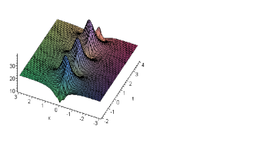
Figure 1. Dynamical evolution of $|q^{[1]}|^{2}$(time periodic breather) with specific parameters $\alpha_{1}=1,\beta_{1}=\dfrac{1}{2},a=-\dfrac{6}{25}$. The trajectory is a line at $x=0$.

Finally, a Taylor series expansion about the breather solution of the FL equation is used to construct the rogue wave of the FL equation in the following way. By letting $a\rightarrow 2({\alpha_{1}}^{2}+{\beta_{1}}^{2})$ in $(\ref{q2j3})$, we obtain the rogue wave solution in the form

$${q}^{[1]}_{rw}=\alpha_{1}\dfrac{s_{2}}{s_{3}}\exp{s_{1}}$$ (21)

with

$$s_{1}=i(2xs+\dfrac{1}{2s}t(4s^{2}-2\frac{-{\beta_{1}}^{2}+s}{s}+4s+1)),$$

$$s_{2}=\hbox to0.0pt{$\displaystyle(t^{2}(-{\beta_{1}}^{2}+s)k_{1}+16x^{2}(-{\beta_{1}}^{2}+s)s^{4}{}$\hss}$$

$${}\mbox{\hskip 22.76228pt}+8tx(-{\beta_{1}}^{2}+s)k_{2}s+2it(-{\beta_{1}}^{2}+s)(12s^{2}+1)s+24ix(-{\beta_{1}}^{2}+s)s^{3}-3s^{3}),$$

$$s_{3}=\hbox to0.0pt{$\displaystyle(t^{2}(-{\beta_{1}}^{2}+s)k_{1}+16x^{2}(-{\beta_{1}}^{2}+s)s^{4}{}$\hss}$$

$${}\mbox{\hskip 22.76228pt}+8tx(-{\beta_{1}}^{2}+s)k_{2}s-2it(-{\beta_{1}}^{2}+s)(4s^{2}-1)s-8ix(-{\beta_{1}}^{2}+s)s^{3}+s^{3})s,$$

$$k_{1}=\hbox to0.0pt{$\displaystyle 64(-{\beta_{1}}^{4}+s{\beta_{1}}^{2})(2{\beta_{1}}^{4}-2s{\beta_{1}}^{2}+s^{2})+128{\beta_{1}}^{8}-256s{\beta_{1}}^{6}{}$\hss}$$

$${}\mbox{\hskip 22.76228pt}+192s^{2}{\beta_{1}}^{4}+(-64s^{3}-16s){\beta_{1}}^{2}+8s^{2}+16s^{4}+1,$$

$$k_{2}=12(-{\beta_{1}}^{4}+s{\beta_{1}}^{2})s+12s{\beta_{1}}^{4}+(-12s^{2}-2){\beta_{1}}^{2}+s+4s^{3},$$

$$s={\alpha_{1}}^{2}+{\beta_{1}}^{2}.$$

By letting $x\rightarrow{\infty},\ t\rightarrow{\infty}$, so $|{q}^{[1]}_{rw}|^{2}\rightarrow$$\dfrac{{\alpha_{1}}^{2}}{({\alpha_{1}}^{2}+{\beta_{1}}^{2})^{2}}$. The maximum amplitude of $|{q}^{[1]}_{rw}|^{2}$ occurs at $t=0$ and $x=0$ and is equal to $\dfrac{9{\alpha_{1}}^{2}}{({\alpha_{1}}^{2}+{\beta_{1}}^{2})^{2}}$,and the minimum amplitude of $|{q}^{[1]}_{rw}|^{2}$ occurs at $t=\pm\dfrac{9({\alpha_{1}}^{2}+{\beta_{1}}^{2})^{2}}{2\sqrt{3({\alpha_{1}}^{2}+4{\beta_{1}}^{2})}{\alpha_{1}}}$ and $x=\mp\dfrac{3(12({\alpha_{1}}^{2}+{\beta_{1}}^{2})^{2}+1)}{8\sqrt{3({\alpha_{1}}^{2}+4{\beta_{1}}^{2})}{\alpha_{1}}}$ and is equal to $0$. Through Figure 2 and Figure 3 of $|{q}^{[1]}_{rw}|^{2}$, the main features (such as large amplitude and local property on (x-t) plane) of the rogue wave are clearly shown.

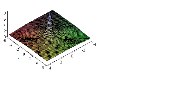
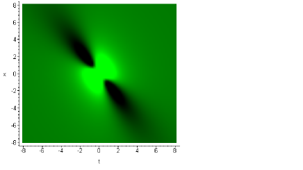
Figure 2. Dynamical evolution of $|{q}^{[1]}_{rw}|^{2}$ with specific parameters $\alpha_{1}=\dfrac{1}{2},\beta_{1}=\dfrac{1}{2}$, in the limit$x\rightarrow{\infty},\ t\rightarrow{\infty}$, so $|{q}^{[1]}_{rw}|^{2}\rightarrow 1$. The maximum amplitude of $|q^{[1]}_{rw}|^{2}$ occurs at $t=0$ and $x=0$ and is equal to 9,and the minimum amplitude of $|q^{[1]}_{rw}|^{2}$ occurs at $t=\pm\dfrac{3\sqrt{15}}{10}$ and $x=\mp\dfrac{2\sqrt{15}}{5}$ and is equal to $0$.

Figure 3. Contour plot of the wave amplitudes of $|{q}^{[1]}_{rw}|^{2}$ with $\alpha_{1}=\dfrac{1}{2},\beta_{1}=\dfrac{1}{2}$.

4. Conclusions

Thus, in this paper, considering FL system of equation which describes nonlinear pulse propagation through single mode optical fiber, the determinant representation of the one-fold DT for the FL system is given eqs.(16) and (17). By choosing pair of eigenvalues in the form $\lambda_{2}=\lambda_{1}^{*}$ and assuming suitable seed solutions, the breather solution and rogue waves of the FL equation are derived in eq. (3) and eq. (21). Our results provide an alternative possibility to observe rogue waves in optical system. From the one-fold DT, it is interesting to observe that the DT of the FL system exhibits the following novelty in comparison with other integrable models like the AKNS and the KN systems: the DT matrix of the FL system has three different terms depending on $\lambda$.

Thus, the DT as well as the rogue wave of the FL system present novel features, in comparison with the DT and rogue wave solutions of the standard integrable systems like the AKNS and the KN systems. The construction of higher order rogue wave of the FL equation by using the determinant representation of the DT will be published elsewhere.

Acknowledgments This work is supported by the NSF of China under Grant No.10971109 and K.C.Wong Magna Fund in Ningbo University. Jingsong He is also supported by Program for NCET under Grant No.NCET-08-0515 and Natural Science Foundation of Ningbo under Grant No.2011A610179. We thank Prof. Yishen Li(USTC,Hefei, China) for his useful suggestions on the rogue wave. J. He thank Prof. A.S.Fokas and Dr. Dionyssis Mantzavino(Cambridge University) for many helps on this paper. KP wishes to thank the DST, DAE-BRNS, UGC, CSIR, Government of India, for the financial support through major projects.

References

- [1] A.S.Fokas,Physica.D. 87 (1995) 145 .
- [2] J.Lenells and A.S.Fokas,Inverse.Probl. 25 (2009) 115006 .
- [3] J.Lenells and A.S.Fokas,Nonlinearity. 22 (2009) 11.
- [4] J.Lenells,J.Nonlinear.Sci. 20 (2010) 709.
- [5] J.Lenells, Stud. Appl. Math.123 (2009) 215.
- [6] G.Neugebauer and R.Meinel, Phys.Lett.A.100 (1984) 467.
- [7] V. B. Matveev, M.A. Salle, Darboux Transfromations and Solitons(Springer-Verlag, Berlin)(1991).
- [8] J.S.He, L.Zhang, Y.Cheng and Y.S.Li, Science in China Series A: Mathematics.12 (2006) 1867.
- [9] Kenji Imai, J.Phys.Soc.Japan.68 (1999) 355.
- [10] H Steudel, J.Phys.A: Math.Gen.36 (2003) 1931.
- [11] S.W. Xu, J.S.He and L.H.Wang, J. Phys. A: Math. Theor. 44 (2011) 305203.
- [12] M.J.Ablowitz, D.J.Kaup, A.C.Newell and H.Segur, Phys.Rev.Lett. 31 (1973) 125.
- [13] M.J.Ablowitz and P.A.Clarkson, Solitons, Nonlinear evolution equations and Inverse scattering (Cambridge: Cambridge University Press) (1991).
- [14] D.J.Kaup and A.C.Newell, J.Math.Phys. 19 (1978) 798.
- [15] C.Kharif and E.Pelinovsky, Eur.J.Mech.B (Fluids). 22 (2003) 603.
- [16] C.Kharif, E.Pelinovsky and A.Slunyaev, Rogue Waves in the Ocean (Berlin: Springer)(2009).
- [17] N. Akhmediev, A. Ankiewicz and M.Taki, Phys. Lett. A. 373 (2009) 675.
- [18] N. Akhmediev, J. M. Soto-Crespo and A. Ankiewicz, Phys. Lett. A. 373 (2009) 2137.
- [19] A.Chabchoub, N.P.Hoffmann and N.Akhmediev, Phys. Rev. Lett. 106 (2011) 204502.
- [20] I.Didenkulova1 and E.Pelinovsky, Nonlinearity. 24 (2011) R1.
- [21] D. H. Peregrine, Water waves, J. Aust. Math. Soc. Ser. B, Appl. Math. 25 (1983) 16.
- [22] Kristian, B.Dysthe and K.Trulsen, Phys Scri. 82 (1999) 48.
- [23] V.E.Zakharov and A.I.Dyachenko, Eur.J.Mech.B (Fluids). 29 (2008) 127.
- [24] V.E.Zakharov and L.A.Ostrovsky, Phys.D. 238 (2009) 540.
- [25] N.N.Akhmediev and V.I.Korneev, Theor. Math. Phys. 69 (1986) 1080.
- [26] Y.C.Ma, Stud.Appl.Math. 60 (1979) 43.
- [27] N. Akhmediev, A.Ankiewicz and J. M. Soto-Crespo,Phys. Rev. E. 80 (2009) 026601.
- [28] Zhenya.Yan, Phys. Lett.A. 374 (2009) 672.
- [29] Boling.Guo,Liming.Ling and Q.P.Liu, Phys.Rev.E 85 (2012) 026607.
- [30] L.H.Ying,Z.Zhuang,E. J.Heller and L.Kaplan, Nonlinearity. 24 (2011) R67.
- [31] Y.Otha, J.K.Yang, Proc. R. Soc. A 468 (2012) 1716.
- [32] Xuan Ni, Wen-Xu Wang and Ying-Cheng Lai, Europhysics.Lett. 96 (2011) 44002.
- [33] N. Akhmediev,J. M. Soto-Crespo and A. Ankiewicz, Phys. Rev. A. 80 (2009) 043818.
- [34] V. Fedun, M.S.Ruderman and R. Erdélyi, Phys. Lett.A. 372 (2008) 6107.
- [35] M.S. Ruderman, Euro. Phys. Jour, 185 (2010) 57.
- [36] W.M.Moslem, P.K.Shukla and B.Eliasson, Euro.Phys.Lett. 96 (2011) 25002.
- [37] D.R.Solli, C.Ropers, P.Koonath and B.Jalali, Nature, 450 (2007) 1054.
- [38] B.Kibler, J. Fatome, C.Finot, G.Millot,F. Dias, G. Genty, N. Akhmediev and J.M. Dudley, Nature.Physics. 6 (2010) 790.
- [39] F.T.Arecchi, U. Bortolozzo,A. Montina and S. Residori, Phys. Rev. Lett. 106 (2011) 153901.
- [40] Adrian Ankiewicz, J. M. Soto-Crespo and Nail Akhmediev, Phys. Rev. E. 81 (2010) 046602.
- [41] Yongsheng Tao and Jingsong He, Phys. Rev. E 85 (2012) 026601.
- [42] Jingsong He, Shuwei XU and Kuppuswamy Porseizan, J.Phys. Soc. Jpn. 81 (2012) 033002.