Genetic theory for cubic graphs

Abstract

We propose a partitioning of the set of unlabelled, connected cubic graphs into two disjoint subsets named genes and descendants, where the cardinality of the descendants is much larger than that of the genes. The key distinction between the two subsets is the presence of special edge cut sets, called crackers, in the descendants. We show that every descendant can be created by starting from a finite set of genes, and introducing the required crackers by special breeding operations. We prove that it is always possible to identify genes that can be used to generate any given descendant, and provide inverse operations that enable their reconstruction. A number of interesting properties of genes may be inherited by the descendant, and we therefore propose a natural algorithm that decomposes a descendant into its ancestor genes. We conjecture that each descendant can only be generated by starting with a unique set of ancestor genes. The latter is supported by numerical experiments.

1 Introduction

In this paper, we study the family $S:=S(N)$ of undirected, unlabelled, connected cubic graphs on $N=2m$ vertices, where $m$ is a positive integer greater or equal to $2$. We recall that a cubic graph has exactly three edges incident on every vertex. In our study we will be concerned with the problem of generating complex cubic graphs by appropriate compositions of simpler cubic graphs in a manner somewhat analogous to genetic “breeding”. This will be achieved with the help of six “breeding operations”. Cubic graphs that cannot be seen as resulting from such operations will be called “genes”, and all other cubic graphs will be called “descendants”. Of course, descendants constitute a majority of cubic graphs. We will prove that every descendant graph can be created from a finite set of genes. Since a lot of the structure in a descendant is inherited from the genes, many properties of those genes are inherited as well. This motivates the introduction of “inverse operations” that, ultimately, decompose a given descendant into a set of “ancestor genes”. Such a decomposition could subsequently be used with other graph theory algorithms to improve solving time.

Undirected cubic graphs have been extensively studied in the literature (e.g., see [Harary 69], [Balaban and Harary 71] [Holton and Sheehan 93]). In particular, there are now programs that enumerate all instances (up to an automorphism) of cubic graphs on $N$ vertices (e.g., see [Meringer 99]). A significant line of research concerns generation of cubic graphs with the help of an exponential generating function (e.g., see [Brinkmann 96], [Meringer 99], [Royle 87]). To the extent that, in this paper, we generate descendant cubic graphs, the present contribution is conceptually, but not methodologically, related to the preceding.

The construction of ancestors and descendants of cubic graphs could be seen as being related to the work of McKay and Royle [McKay and Royle 86]. However, a feature of our approach is that all ancestors and descendants remain in the class of cubic graphs, and collectively constitute the entire set of connected cubic graphs. This enables us to study those properties of cubic graphs that may be “inherited” from simpler cubic graphs. Furthermore, the construction methods are quite different from those in [McKay and Royle 86]. The work of Batagelj [Batagelj 86] is also similar to ours in that it is concerned with the generation of complex cubic graphs from simpler cubic graphs, where the former maintain the properties of the latter. In fact, some of the generating rules given in [Batagelj 86] are analogous to some of the breeding operations in this paper. However, the two approaches differ in that Batagelj’s approach involves starting with a single cubic graph and replacing particular structures within the graph sequentially. In our approach, the majority of development occurs by combining multiple cubic graphs together, with the resulting graph being more complex than both parents.

Importantly, preliminary numerical experimentation revealed a surprising “unique ancestors property” that is either very common or, as we believe, universal. Namely, we conjecture that: Given any descendant cubic graph $G_{D}$ there exists a unique set of genes from which $G_{D}$ can be derived by a finite sequence of the six breeding operations. Of course, there may well be a multitude of sequences of breeding operations that lead from the ancestor genes to $G_{D}$. However, if the above conjecture holds, then all possible decomposition pathways of $G_{D}$ into its ancestor genes will ultimately lead to a unique set of ancestor genes.

2 Preliminaries

At the conclusion of this manuscript, we conjecture that any given descendant can be obtained via our approach through a particular set of ancestor genes, and provide numerical evidence supporting this conjecture. If true, this conjecture, combined with the proof of existence of ancestor genes for any descendant, implies that our approach permits a unique decomposition for every cubic graph.

A standard concept in graph theory is that of edge connectivity. In the simple case in which removing a single, specific edge would disconnect the graph, that edge is called a bridge. Extending this notion a set of edges $EC$ constitutes an edge cut if their removal disconnects the graph. The smallest cardinality of an edge cut in a given graph $G$ is defined to be the edge-connectivity of that graph. Of course, cubic graphs can be $k-$edge-connected for only three values of $k$: $1,2$ or $3$.

We note, however, that in some $3-$edge-connected cubic graphs (e.g., the famous Petersen graph, see Figure 2) the removal of any minimal edge cut set isolates a single vertex. Arguably, such a partition of vertices is in a sense degenerate, and prevents a more refined classification of cubic graphs. To address this problem and achieve a finer classification we introduce a special class of edge cut sets that we name crackers. The latter are defined as follows.

Definition 2.1.

An edge cut set of a cubic graph $\Gamma$ consisting of $k$ edges is a $k$-cracker if no two edges are adjacent in the sense of being incident on the same vertex, and no proper subset of these edges disconnects the graph.

Lemma 2.2.

The removal of a cracker from a connected graph results in exactly two disjoint components.

Proof.  Since any cracker is an edge cut set, the removal of a cracker must result in at least two disjoint components. Assume there exists a cracker $C=\{e_{1},\ldots,e_{k}\}$ whose removal results in more than two disjoint components. We can think of the removal of $C$ as a series of individual edge removals, for each edge in $C$. It is clear that the removal of a single edge cannot result in more than one additional disjoint component. Therefore, after removing edges $e_{1},\ldots,e_{k-1}$, but before removing edge $e_{k}$, there must already be at least two disjoint components. However, this implies that a proper subset of $C$ also disconnects the graph, which violates Definition 2.1. Therefore, $C$ is not a cracker, and the initial assumption is false.    $\Box$

Of course, any cracker is not only an edge cut set, but in fact a cyclic edge cut set. This is clear because its removal disconnects the graph into two connected subgraphs, each of which must contain at least three vertices. Since each remaining vertex has degree at least two (as only non-adjacent edges were removed), these connected subgraphs must contain cycles. It is then clear that a minimal cyclic edge cut set in a given cubic graph is a cracker of minimal size for that graph. However, larger cyclic edge cut sets may contain adjacent edges, and therefore not all cyclic edge cut sets are crackers.

We recall that the girth, $g$, of a graph is the length of the shortest (nontrivial) cycle in the graph. In many cases, a nontrivial cycle determining a cubic graph’s girth automatically defines a $g$-cracker made up of edges that are not in the cycle but which have one vertex on the cycle. However, many graphs have crackers of size less than $g$. For instance, it is easy to see that in the graph given in Figure 1, $g=3$ but the edges $e_{1}$ and $e_{2}$ form a $2$-cracker and no $1$-cracker exists in this graph.

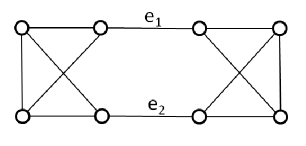
Figure 1: An 8-vertex cubic graph with girth $3$ and the two cracker $\{e_{1},e_{2}\}$

We note also that there are only two connected cubic graphs, on $4$ and $6$ vertices respectively, that contain no crackers at all (see Figure 3 and the discussion in Section 3).

Remark.

Note that, since the minimal cyclic edge cut set in a cubic graph is a cracker, it is clear that for any given cubic graph, the cyclic edge connectivity is equal to the size of the smallest cracker in that graph. For the sake of simplifying the notation, we will refer to a cyclically $k$-connected graph as a C$k$-connected graph. The class of all C$k$-connected cubic graphs on $N$ vertices will be denoted by $S_{k}(N)$, or simply by $S_{k}$, when the number of vertices is fixed.

We note that the famous Petersen graph is C5-connected in the above sense (see Figure 2), as the edges connecting the “inner-star” to the outer boundary form one of a number of $5-$crackers, and no smaller crackers exist in this graph.

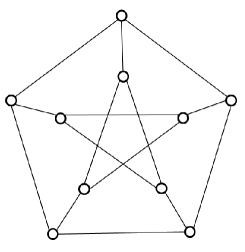
Figure 2: Petersen graph which is C5-connected

3 Motivation

It follows immediately from Remark Remark that (for fixed $N\geq 8$) the class $C$ of connected cubic graphs can be partitioned as

$$S=\bigcup_{i=1}^{M}S_{i},$$

where $M\leq\displaystyle\frac{N}{2}$. The choice of upper bound is conservative because at most $\displaystyle\frac{N}{2}$ non-adjacent edges can be chosen in any graph of size $N$, but in reality it is likely that far fewer than $\displaystyle\frac{N}{2}$ partitions will be required for any given $N$. For instance, when $N=20$, $M=6$.

Definition 3.1.

If a cubic graph $\Gamma$ is C$k$-connected for $k\geq 4$, we call it a gene. Otherwise, we call $\Gamma$ a descendant.

The reasoning behind the choice of names gene and descendant is made clear in Section 4, where we demonstrate that any descendant can be obtained from a set of genes, through the use of prescribed breeding operations that introduce crackers into a descendant. Experiments have shown that genes are far less numerous than descendants.

It was mentioned earlier that two cubic graphs, namely the 4-vertex gene $\Gamma_{4}^{*}$ and the 6-vertex gene $\Gamma_{6}^{*}$, contain no crackers at all. These two graphs can be seen in Figure 3. The following lemma proves that every other cubic graph contains at least one cracker, and that the size of the smallest cracker is bounded above by the girth of the graph.

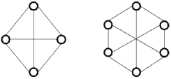
Figure 3: Cubic graphs $\Gamma_{4}^{*}$ and $\Gamma_{6}^{*}$, which contain no crackers

Lemma 3.2.

Except for $\Gamma_{4}^{*}$ and $\Gamma_{6}^{*}$, all connected cubic graphs contain at least one cracker of size no more than the girth $g$ of the graph.

Proof.  The cases of $\Gamma_{4}^{*}$ and $\Gamma_{6}^{*}$ can be confirmed by inspection. There is one other cubic graph containing 6 vertices, with girth 3, which contains a 3-cracker, as displayed in Figure 4. So the lemma is true for $N<8$.

For any cubic graph containing 8 or more vertices, it was proved in Lou et al [Lou et al. 01] that there exists at least one cyclic edge cut set of size $g$. The smallest cyclic edge cut set in a cubic graph is a cracker, so it is clear that the smallest cracker can be of size no bigger than $g$.    $\Box$

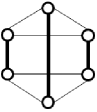
Figure 4: A 6-vertex cubic graph, with girth 3, which contains a 3-cracker comprising the highlighted edges

In Section 5, it is proved that any descendant graph can be obtained from a set of genes. It is our hope that descendants inherit many of their properties from the genes used to construct them. If so, any analysis of such a descendant could be reduced to the problem of analysing the component genes, which are often much smaller than the descendant. The subsequent investigation of graph theoretic properties in sets of genes is a natural topic for future research.

One such graph theoretic property of interest is that of Hamiltonicity, that is, the property of containing a simple cycle of length equal to the number of vertices in the graph. We observe that non-Hamiltonian genes are extremely rare. Even excluding the (trivially non-Hamiltonian) bridge graphs, non-Hamiltonian descendants constitute a large majority of the remaining non-Hamiltonian graphs; see Table 1. The second column of that table, labelled by $\mbox{NH}_{1}$, lists the percentages of bridge graphs relative to the total cardinality of non-Hamiltonian graphs, denoted by NH. The third column labelled by $\mbox{NH}_{2+}:=\mbox{NH}\setminus\mbox{NH}_{1}$, lists the percentages of graphs two or more cyclically edge connected relative to the cardinality of NH. The fourth column labelled by $\mbox{NH}_{4+}$, lists the percentages of graphs four or more cyclically edge connected relative to the cardinality of NH. Finally, the fifth column labelled by $\mbox{NH}_{4+}/\mbox{NH}_{2+}$, lists the percentages of graphs four or more cyclically edge connected relative to the cardinality of all non-bridge, non-Hamiltonian, graphs in $\mbox{NH}_{2+}$. We shall define graphs in $\mbox{NH}_{4+}$ as mutants, a name that properly reflects their exceptionality. For instance, we note from the fourth column of Table 1 that with $N=18$ only $0.12$ of one percent are mutants, which corresponds to two (out of 1666) non-Hamiltonian cubic graphs on $18$ vertices. These two mutants are the famous Blanus̆a Snarks [Blanus̆a 46].

In fact, it is no coincidence that the Blanus̆a Snarks appear as mutants in this framework. In Read and Wilson [Read and Wilson 98], the definition of an irreducible Snark is given as a cubic graph with edge chromatic number of 4, girth 5 or more, and not containing three edges whose deletion results in a disconnected graph, each of whose components is nontrivial. This final condition, along with the well known fact that all Snarks are non-Hamiltonian, is akin to our definition of a mutant. Therefore, the set of all mutants is a superset of the set of all irreducible Snarks. However, some non-Snark mutants do exist, and therefore have either girth 4 or an edge chromatic number of 3 (or both). In particular, the BH-Mutant, displayed in Figure 5 is the smallest non-Snark mutant, and has an edge chromatic number of 3. There are 16 further non-Snark mutants of size 22, one of which is the Zircon-Mutant, also displayed in Figure 5. The Zircon-Mutant also has an edge chromatic number of 3.

	$\mbox{NH}_{1}$	$\mbox{NH}_{2+}$	NH4+	$\mbox{NH}_{4+}/\mbox{NH}_{2+}$
$10$ Vertex	$50.00\%$	$50.00\%$	$50.00\%$	$100\%$
$12$ Vertex	$80.00\%$	$20.00\%$	$0\%$	$0\%$
$14$ Vertex	$82.86\%$	$17.14\%$	$0\%$	$0\%$
$16$ Vertex	$84.93\%$	$15.07\%$	$0\%$	$0\%$
$18$ Vertex	$86.13\%$	$13.86\%$	$0.12\%$	$0.86\%$
$20$ Vertex	$87.40\%$	$12.60\%$	$0.05\%$	$0.38\%$
$22$ Vertex	$88.59\%$	$11.41\%$	$0.02\%$	$0.21\%$

Table 1: Distribution of Non-Hamiltonian (NH) C$k$-connected graphs

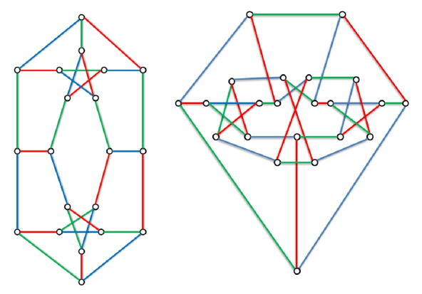
Figure 5: BH-Mutant which is a girth 5, C4-connected non-Hamiltonian non-Snark mutant containing 20 vertices, and Zircon-Mutant which is a girth 5, C5-connected non-Hamiltonian non-Snark mutant containing 22 vertices. The colours identify Tait Colorings

4 Breeding and parthenogenic operations

From Definition 3.1, it is clear that genes do not contain any 1-crackers, $2$-crackers, or $3$-crackers. Collectively, we refer to 1-crackers, $2$-crackers and $3$-crackers as cubic crackers. As a corollary, descendants must contain at least one cubic cracker. It then seems plausible that we might be able to construct any given descendant by combining two or more cubic graphs together in such a fashion as to create the cubic crackers present in that descendant graph. Since there are three different types of cubic crackers, we define three breeding operations that map two cubic graphs to a single descendant by inserting a cubic cracker between them in such a fashion as to retain cubicity. In such a case, we say that the descendant has been obtained by breeding. We refer to the original two cubic graphs as the parents of the descendant graph, and likewise the descendant graph is the child of the two parents.

Note that the following operations are defined only for cubic graphs. Although they work for disconnected cubic graphs, in this manuscript we are interested only in connected cubic graphs, and make the assumption that all input graphs are indeed connected and cubic.

4.1 Breeding operations

Definition 4.1.

A type 1 breeding operation is a function $\mathcal{B}_{1}$ defined on the tuple $(\Gamma_{1},\Gamma_{2},e_{1},e_{2})$, where $\Gamma_{1}=\left<V_{1},E_{1}\right>$ and $\Gamma_{2}=\left<V_{2},E_{2}\right>$ are cubic graphs, and furthermore, $e_{1}=(a,b)\in E_{1}$ and $e_{2}=(c,d)\in E_{2}$. This function maps such a tuple onto another tuple $(\Gamma_{D},e)$ as follows

$$\mathcal{B}_{1}(\Gamma_{1},\Gamma_{2},e_{1},e_{2}) = (\Gamma_{D},e),$$

where $\Gamma_{D}=\left<V_{D},E_{D}\right>$ and $\{e=(v_{1},v_{2})\}\in E_{D}$. The new set of vertices is $V_{D}=V_{1}\;\cup\;V_{2}\;\cup\;v_{1}\;\cup\;v_{2}$. The new set of edges is $E_{D}=(E_{1}\backslash e_{1})\;\cup\;(E_{2}\backslash e_{2})\;\cup\;\{(a,v_{1}),(b,v_{1}),(c,v_{2}),(d,v_{2}),(v_{1},v_{2})\}$.

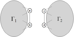
Figure 6: Graphs $\Gamma_{1}$, $\Gamma_{2}$ and $\Gamma_{D}$ as described in Definition 4.1

Note that a type 1 breeding operation always outputs a bridge graph (that is, a C1-connected graph). See Figure 6 for an illustration.

Definition 4.2.

A type 2 breeding operation is a function $\mathcal{B}_{2}$ defined on the tuple $(\Gamma_{1},\Gamma_{2},e_{1},e_{2})$, where $\Gamma_{1}=\left<V_{1},E_{1}\right>$ and $\Gamma_{2}=\left<V_{2},E_{2}\right>$ are cubic graphs, and furthermore, $e_{1}=(a,b)\in E_{1}$ and $e_{2}=(c,d)\in E_{2}$ and neither edge is a $1$-cracker. This function maps such a tuple onto another tuple $(\Gamma_{D},e_{3},e_{4})$ as follows

$$\mathcal{B}_{2}(\Gamma_{1},\Gamma_{2},e_{1},e_{2}) = (\Gamma_{D},e_{3},e_{4}),$$

where $\Gamma_{D}=\left<V_{D},E_{D}\right>$ and $\{e_{3}=(a,c),e_{4}=(b,d)\}\in E_{D}$. The new set of vertices is $V_{D}=V_{1}\;\cup\;V_{2}$. The new set of edges is $E_{D}=(E_{1}\backslash e_{1})\;\cup\;(E_{2}\backslash e_{2})\;\cup\;\{(a,c),(b,d)\}$.

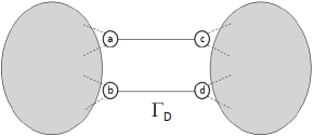
Figure 7: Graphs $\Gamma_{1}$, $\Gamma_{2}$ and $\Gamma_{D}$ as described in Definition 4.2

Clearly $\Gamma_{D}$ contains the $2$-cracker $\{(a,c),(b,d)\}$. See Figure 7 for an illustration. Note also that a type 2 breeding operation always creates a 2-edge-connected descendant, unless either of $\Gamma_{1}$ or $\Gamma_{2}$ is 1-edge-connected (in which case, $\Gamma_{D}$ is also 1-edge-connected).

Definition 4.3.

A type 3 breeding operation is a function $\mathcal{B}_{3}$ defined on the tuple $(\Gamma_{1},\Gamma_{2},v_{1},v_{2},a,b,\\ c,d,e,f)$, where $\Gamma_{1}=\left<V_{1},E_{1}\right>$ and $\Gamma_{2}=\left<V_{2},E_{2}\right>$ are cubic graphs, and furthermore, $v_{1}\in V_{1}$ is incident to vertices $a$ , $b$ and $c\in V_{1}$ and $v_{2}\in V_{2}$ is incident to vertices $d$, $e$ and $f\in V_{2}$. None of the edges adjacent to $v_{1}$ or $v_{2}$ are $1$-crackers. This function maps such a tuple onto another tuple $(\Gamma_{D},e_{1},e_{2},e_{3})$ as follows

$$\mathcal{B}_{3}(\Gamma_{1},\Gamma_{2},v_{1},v_{2},a,b,c,d,e,f) = (\Gamma_{D},e_{1},e_{2},e_{3}),$$

where $\Gamma_{D}=\left<V_{D},E_{D}\right>$, and also, $\{e_{1}=(a,d),e_{2}=(b,e),e_{3}=(c,f)\}\in E_{D}$). The new set of vertices is $V_{D}=(V_{1}\backslash v_{1})\;\cup\;(V_{2}\backslash v_{2})$. The new set of edges is $E_{D}=(E_{1}\backslash\{(v_{1},a),(v_{1},b),(v_{1},c)\})\;\cup\;(E_{2}\backslash\{(v_{2},d),(v_{2},e),(v_{2},f)\})\cup\;\{(a,d),(b,e),(c,f)\}$.

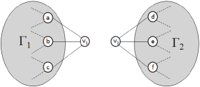
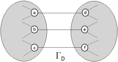
Figure 8: Graphs $\Gamma_{1}$, $\Gamma_{2}$ and $\Gamma_{D}$ as described in Definition 4.3

See Figure 8 for an illustration of type 3 breeding.

4.2 Parthenogenic operations

In addition to the preceding three breeding operations, we also define three parthenogenic operations. These are operations that map a single descendant to a new, more complex, descendant by replacing a cracker in the original descendant with two new crackers. We say that such a new descendant has been obtained from parthenogenesis. For simplicity of terminology, we again refer to the original descendant as the parent of the new descendant, and likewise we refer to the new descendant as the child of the original descendant. Also for simplicity of terminology, we refer to the the three breeding operations and the three parthenogenic operations collectively as the six breeding operations.

Definition 4.4.

A type 1 parthenogenic operation is a function $\mathcal{P}_{1}$ defined on the tuple $(\Gamma_{1},e_{1})$ where $\Gamma_{1}=\left<V_{1},E_{1}\right>$ is a bridge graph and $e_{1}=(a,b)\in E_{1}$ is a 1-cracker. This function maps such a tuple onto another tuple $(\Gamma_{D},v_{1},v_{4})$ as follows

$$\mathcal{P}_{1}(\Gamma_{1},e_{1}) = (\Gamma_{D},v_{1},v_{4}),$$

where $\Gamma_{D}=\left<V_{D},E_{D}\right>$ and $\{v_{1},v_{4}\}\in V_{D}$. The new set of vertices is $V_{D}=V_{1}\;\cup\;\{v_{1},v_{2},v_{3},v_{4}\}$. The new set of edges is $E_{D}=(E_{1}\backslash e_{1})\;\cup\;\{(a,v_{1}),(v_{1},v_{2}),(v_{1},v_{3}),(v_{2},v_{3}),(v_{2},v_{4}),(v_{3},v_{4}),\\ (v_{4},b)\}$. This process inserts an additional $1$-cracker into $\Gamma_{D}$.

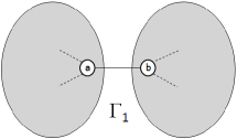
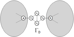
Figure 9: Graphs $\Gamma_{1}$ and $\Gamma_{D}$ as described in Definition 4.4

We refer to the subgraph $\Gamma_{S}=\left<\{v_{1},v_{2},v_{3},v_{4}\},\{(v_{1},v_{2}),(v_{1},v_{3}),(v_{2},v_{3}),(v_{2},v_{4}),(v_{3},v_{4})\}\right>$ as the parthenogenic diamond, and say that a type 1 parthenogenic operation inserts a parthenogenic diamond into a bridge. See Figure 9 for an illustration.

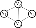
Figure 10: A parthenogenic diamond

Definition 4.5.

A type 2 parthenogenic operation is a function $\mathcal{P}_{2}$ defined on the tuple $(\Gamma_{1},e_{1},e_{2})$ where $\Gamma_{1}=\left<V_{1},E_{1}\right>$ is a cubic graph containing a $2$-cracker comprising two edges $e_{1}=(a,b)$ and $e_{2}=(c,d)$. This function maps such a tuple onto another tuple $(\Gamma_{D},v_{1},v_{2})$ as follows

$$\mathcal{P}_{2}(\Gamma_{1},e_{1},e_{2}) = (\Gamma_{D},v_{1},v_{2}),$$

where $\Gamma_{D}=\left<V_{D},E_{D}\right>$ and $\{v_{1},v_{2}\}\in V_{D}$. The new set of vertices is $V_{D}=V_{1}\;\cup\;\{v_{1},v_{2}\}$. The new set of edges is $E_{D}=(E_{1}\backslash\{e_{1},e_{2}\})\;\cup\;\{(a,v_{1}),(b,v_{1}),(c,v_{2}),(d,v_{2}),(v_{1},v_{2})\}$. This process inserts an additional $2$-cracker into $\Gamma_{D}$.

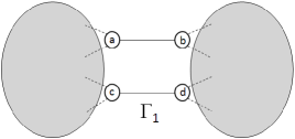
Figure 11: Graphs $\Gamma_{1}$ and $\Gamma_{D}$ as described in Definition 4.5

We refer to the subgraph $\Gamma_{S}=\left<\{v_{1},v_{2}\},(v_{1},v_{2})\right>$ as the parthenogenic bridge, and say that a type 2 parthenogenic operation inserts a parthenogenic bridge into a $2$-cracker. See Figure 11 for an illustration.

Figure 12: A parthenogenic bridge

Definition 4.6.

A type 3 parthenogenic operation is a function $\mathcal{P}_{3}$ defined on the tuple $(\Gamma_{1},a)$ where $\Gamma_{1}=\left<V_{1},E_{1}\right>$ is a bridge graph and $a\in V_{1}$ is a vertex incident to a $1$-cracker composing an edge $e_{1}=(a,b)\in E_{1}$ and is adjacent to vertices $c$ and $d\in V_{1}$. This function maps such a tuple onto another tuple $(\Gamma_{D},a,v_{1},v_{2})$ as follows

$$\mathcal{P}_{3}(\Gamma_{1},a) = (\Gamma_{D},a,v_{1},v_{2}),$$

where $\Gamma_{D}=\left<V_{D},E_{D}\right>$ and $\{a,v_{1},v_{2}\}\in V_{D}$. The new set of vertices is $V_{D}=V_{1}\;\cup\;\{v_{1},v_{2}\}$. The new set of edges is $E_{D}=(E_{1}\backslash\{(a,c),(a,d)\})\;\cup\;\{(a,v_{1}),(a,v_{2}),(v_{1},v_{2}),(v_{1},c),(v_{2},d)\}$.

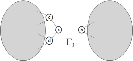
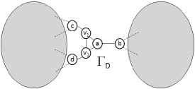
Figure 13: Graphs $\Gamma_{1}$ and $\Gamma_{D}$ as described in Definition 4.6

We refer to the subgraph $\Gamma_{S}=\left<\{a,v_{1},v_{2}\},\{(a,v_{1}),(a,v_{2}),(v_{1},v_{2})\}\right>$ as the parthenogenic triangle, and say that a type 3 parthenogenic operation inserts a parthenogenic triangle next to the 1-cracker. See Figure 13 for an illustration.

Figure 14: A parthenogenic triangle

Lemma 4.7.

A child graph resulting from any of the six breeding operations is connected.

Proof.  The nature of the six breeding operations is that the parent graphs are mostly unaltered, and are changed only in a neighbourhood of the introduced cubic cracker. Therefore, we can focus just on these areas. Since the parent graphs are (by definition) connected to begin with, we only need to be concerned with which edges, present in the parent graphs, are not present in the child graph.

For the cases of type 2 breeding, and types 1 and 2 parthenogenesis, only a single edge from the parent graph (or from each of the parent graphs in the case of type 2 breeding) is missing in the child graph. By definition this edge cannot be a 1-cracker, and therefore, the parent graphs remain connected, and by construction it is clear that the adjoining cracker ensures the child graph is also connected.

For type 1 breeding, only a single edge is removed from each parent graph. If neither edge is a 1-cracker, then the argument in the previous paragraph can be used to show the child graph is connected. However, it is possible that one or both removed edges could be 1-crackers. If so, the corresponding parent graphs become disconnected. However, if this is the case, the graphs are reconnected by the introduction of vertices $v_{1}$ and $v_{2}$ (see Definition 4.1). It is then clear by construction that the adjoining cracker ensures the child graph is also connected.

For type 3 breeding, a vertex is removed from both parent graphs. From Definition 4.3, we know that none of the edges adjacent to these two vertices constitute 1-crackers. Therefore, the removal of these vertices cannot disconnect either graph. By construction it is then clear that the adjoining cracker ensures the child graph is also connected.

Finally, for type 3 parthenogenesis, although two (adjacent) edges from the parent graph are missing in the child graph, it is clear from the latter’s construction that this can not result in a disconnected descendant.    $\Box$

4.3 Inverse breeding and inverse parthenogenic operations

For some tuples $(\Gamma_{D},e)$ where $\{e\}\in E_{D}$ is a $1$-cracker, the inverse operation $\mathcal{B}^{-1}_{1}(\Gamma_{D},e)=(\Gamma_{1},\Gamma_{2},e_{1},e_{2})$ is well defined. In such a case $\{e\}$ is called an irreducible $1$-cracker. If not $\{e\}$ will be called a reducible $1$-cracker. Similarly if the inverse operation $\mathcal{B}^{-1}_{2}(\Gamma_{D},e_{3},e_{4})=(\Gamma_{1},\Gamma_{2},e_{1},e_{2})$ is well defined, where $\{e_{3},e_{4}\}\in E_{D}$ is a $2$-cracker, the 2-cracker is called an irreducible $2$-cracker and reducible $2$-cracker otherwise. We will show later that the inverse operation $\mathcal{B}^{-1}_{3}(\Gamma_{D},e_{1},e_{2},e_{3})=(\Gamma_{1},\Gamma_{2},v_{1},v_{2},a,b,c,d,e,f)$ is always defined where $\{e_{1},e_{2},e_{3}\}\in E_{D}$ is a $3$-cracker. Therefore every 3-cracker is irreducible.

Definition 4.8.

Whenever a cubic cracker is irreducible one of the equations (1), (2) and (3) defines the corresponding inverse breeding operation $\mathcal{B}^{-1}_{1}(.)$ , $\mathcal{B}^{-1}_{2}(.)$ or $\mathcal{B}^{-1}_{3}(.)$. The two cubic graphs $(\Gamma_{1},\Gamma_{2})$ from the tuple produced by these operations are parents of $\Gamma_{D}$. In particular,

$$\mathcal{B}^{-1}_{1}(\Gamma_{D},e)=(\Gamma_{1},\Gamma_{2},e_{1},e_{2})$$ (1)

where $\Gamma_{D}$, $e$, $\Gamma_{1}$, $\Gamma_{2}$, $e_{1}$ and $e_{2}$ are defined in Definition 4.1. Similarly,

$$\mathcal{B}^{-1}_{2}(\Gamma_{D},e_{3},e_{4})=(\Gamma_{1},\Gamma_{2},e_{1},e_{2})$$ (2)

where $\Gamma_{D}$, $e_{3}$, $e_{4}$, $\Gamma_{1}$, $\Gamma_{2}$, $e_{1}$ and $e_{2}$ are defined in Definition 4.2. Also,

$$\mathcal{B}^{-1}_{3}(\Gamma_{D},e_{1},e_{2},e_{3})=(\Gamma_{1},\Gamma_{2},v_{1},v_{2},a,b,c,d,e,f)$$ (3)

where $\Gamma_{D}$, $e_{1}$, $e_{2}$, $e_{3}$, $\Gamma_{1}$, $\Gamma_{2}$, $v_{1}$, $v_{2}$, $a$, $b$, $c$, $d$, $e$ and $f$ are defined in Definition 4.3.

Similarly, inverse parthenogenic operations can be defined as follows.

Definition 4.9.

Equations (4), (5) and (6) define the corresponding inverse parthenogenic operations $\mathcal{P}^{-1}_{1}(.)$ , $\mathcal{P}^{-1}_{2}(.)$ or $\mathcal{P}^{-1}_{3}(.)$. The cubic graph $(\Gamma_{1})$ from the tuple produced by these operations is a parent of $\Gamma_{D}$. In particular,

$$\mathcal{P}^{-1}_{1}(\Gamma_{D},v_{1},v_{4})=(\Gamma_{1},e_{1}),$$ (4)

where $\Gamma_{D}$, $v_{1}$, $v_{4}$, $\Gamma_{1}$ and $e_{1}$ are defined in Definition 4.4. Similarly,

$$\mathcal{P}^{-1}_{2}(\Gamma_{D},v_{1},v_{2})=(\Gamma_{1},e_{1},e_{2}),$$ (5)

where $\Gamma_{D}$, $v_{1}$, $v_{2}$, $\Gamma_{1}$, $e_{1}$ and $e_{2}$ are defined in Definition 4.5. Also,

$$\mathcal{P}^{-1}_{3}(\Gamma_{D},a,v_{1},v_{2})=(\Gamma_{1},a),$$ (6)

Where $\Gamma_{D}$, $a$, $\Gamma_{1}$, $\Gamma_{2}$, $v_{1}$ and $v_{2}$ are defined in Definition 4.6.

Collectively, we refer to the three inverse breeding operations and the three inverse parthenogenic operations as the six inverse operations.

It is important to note that the six breeding operations and the six inverse operations presented here are not entirely new, and have been used in various forms in other cubic graph generation routines. For example, type 2 parthenogenesis induces an H-subgraph which is well-studied in literature (e.g. see Ore [Ore 67]). Type 1 inverse parthenogenesis and type 1 inverse breeding appear as Operation $O_{2}(K_{4})$ and Operations $\mathcal{R}$ respectively in Ding and Kanno [Ding and Kanno 06]. Types 1 and 2 parthenogenesis appear in Brinkmann [Brinkmann 96]. All of the six breeding operations except type 3 breeding appear in some sense as generating rules in Batagelj [Batagelj 86], specifically generating rules P1, P2, P3, P4 an P8. However, all of the above works involve growing the complexity of a single graph by the evolution of subgraphs, rather than combining several cubic graphs together. In addition, the operations in the above works that are analogous to our parthenogenic operations are not confined to the same conditions as ours (that is, they must occur on $1$-crackers and $2$-crackers). Little consideration is given in the above works to procedures that are analogous to our inverse operations. The benefits and potency of the particular set of breeding and inverse operations that we have detailed in this section are demonstrated in the following section.

5 Results

The following three propositions relate to the different possible methods of creation of cubic crackers by the six breeding operations, and are used in the proof of the main theorem for this section, Theorem 5.5.

Proposition 5.1.

Any descendant involving a 1-cracker can be obtained from either type 1 breeding, type 1 parthenogenesis, or type 3 parthenogenesis.

Proof.   Consider a descendant $\Gamma_{D}=\left<V_{D},E_{D}\right>$ containing a 1-cracker comprising an edge $(v_{1},v_{2})$. Since $\Gamma_{D}$ is cubic, $v_{1}$ and $v_{2}$ will both be adjacent to two more vertices, say $\{a,b\}$ and $\{c,d\}$ respectively. Since the 1-cracker comprises edge $(v_{1},v_{2})$, we know that $\{a,b\}$ and $\{c,d\}$ are disjoint sets. Then, we can consider two cases.

Case 1: The edges $(a,b)$ and $(c,d)$ are not present in $\Gamma_{D}$. In this case, the 1-cracker is irreducible. Suppose the bridge $(v_{1},v_{2})$ is removed from $\Gamma_{D}$, separating the graph into two subgraphs, $\Gamma_{S1}=\left<V_{S1},E_{S1}\right>$ and $\Gamma_{S2}=\left<V_{S2},E_{S2}\right>$. Without loss of generality, we assume that $v_{1}\in V_{S1}$, and $v_{2}\in V_{S2}$. Then, we define a cubic graph $\Gamma_{1}=\left<V_{1},E_{1}\right>$, where $V_{1}=V_{S1}\backslash v_{1}$ and $E_{1}=(E_{S1}\backslash\{(a,v_{1}),(b,v_{1})\})\;\cup\;(a,b)$. Similarly, we define a second cubic graph $\Gamma_{2}=\left<V_{2},E_{2}\right>$, where $V_{2}=V_{S2}\backslash v_{2}$ and $E_{2}=(E_{S2}\backslash\{(c,v_{2}),(d,v_{2})\})\;\cup\;(c,d)$. Then, $\Gamma_{D}$ can be obtained from the type 1 breeding operation $\mathcal{B}_{1}(\Gamma_{1},\Gamma_{2},(a,b),(c,d))$.

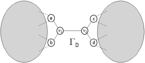
Figure 15: Graphs $\Gamma_{1}$, $\Gamma_{2}$ and $\Gamma_{D}$ as described in Case 1 of Proposition 5.1

Case 2: At least one of the edges $(a,b)$ or $(c,d)$ is present in $\Gamma_{D}$. In this case, the 1-cracker cannot be obtained from a type 1 breeding operation, as such an operation would remove these edges. A 1-cracker of this type is, therefore, reducible. If both edges are present, we can focus on either one. Without loss of generality, we will assume that edge $(a,b)\in E_{D}$. Then, since $\Gamma_{D}$ is cubic, and vertices $a$ and $b$ are both adjacent to vertex $v_{1}$ and to each other, they will also be adjacent to one more vertex each, say vertices $e$ and $f$ respectively. Note that is is possible that $e=f$, so we need to consider the cases separately.

Case 2.1: $e=f$. Then, both edges $(a,e)$ and $(b,e)$ are in $E_{D}$, as seen in the right panel of Figure 16. Since $\Gamma_{D}$ is cubic, vertex $e$ is adjacent to a third vertex, say $g$. Clearly, edge $(e,g)$ is a bridge, since edge $(v_{1},v_{2})$ is a bridge. Then, we define a cubic graph $\Gamma_{1}=\left<V_{1},E_{1}\right>$, where $E_{1}=(E_{D}\backslash\{(v_{1},v_{2}),(a,v_{1}),(b,v_{1}),(a,b),(a,e),(b,e),(e,g)\})\;\cup\;(g,v_{2})$ and $V_{1}=V_{D}\backslash\{v_{1},a,b,e\}$. We can then obtain $\Gamma_{D}$ from the type 1 parthenogenic operation $\mathcal{P}_{1}(\Gamma_{1},(g,v_{2}))$.

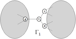
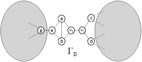
Figure 16: Graphs $\Gamma_{1}$ and $\Gamma_{D}$ as described in Case 2.1 of Proposition 5.1

Case 2.2: $e\neq f$. Then, as illustrated in Figure 17, we define a cubic graph $\Gamma_{1}=\left<V_{1},E_{1}\right>$, where $E_{1}=(E_{D}\backslash\{(a,v_{1}),(b,v_{1}),(a,b),(a,e),(b,f)\})\;\cup\;\{(e,v_{1}),(f,v_{1})\}$ and $V_{1}=V_{D}\backslash\{a,b\}$. Then, we can obtain $\Gamma_{D}$ from the type 3 parthenogenic operation $\mathcal{P}_{3}(\Gamma_{1},v_{1})$.    $\Box$

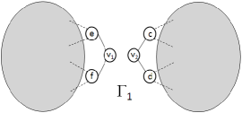
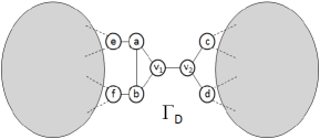
Figure 17: Graphs $\Gamma_{1}$ and $\Gamma_{D}$ as described in Case 2.2 of Proposition 5.1

Proposition 5.2.

Any descendant involving a $2$-cracker can be obtained from either type 1 breeding, type 2 breeding, type 1 parthenogenesis, type 2 parthenogenesis, or type 3 parthenogenesis.

Proof.   Consider a descendant $\Gamma_{D}=\left<V_{D},E_{D}\right>$ containing a $2$-cracker comprising edges $(v_{1},v_{2})$ and $(v_{3},v_{4})$. We consider two cases.

Case 1: Neither edge $(v_{1},v_{3})$ nor $(v_{2},v_{4})$ are not present in $\Gamma_{D}$, as illustrated in Figure 18. In this case, the 2-cracker is irreducible. Suppose the edges $(v_{1},v_{2})$ and $(v_{3},v_{4})$ are removed from $\Gamma_{D}$, separating the graph into two subgraphs $\Gamma_{S1}=\left<V_{S1},E_{S1}\right>$ and $\Gamma_{S2}=\left<V_{S2},E_{S2}\right>$. Without loss of generality, we assume that $v_{1},v_{3}\in V_{S1}$ and $v_{2},v_{4}\in V_{S2}$. Then, we define a cubic graph $\Gamma_{1}=\left<V_{1},E_{1}\right>$, where $V_{1}=V_{S1}$ and $E_{1}=E_{S1}\;\cup\;(v_{1},v_{3})$. Similarly, we define a second cubic graph $\Gamma_{2}=\left<V_{2},E_{2}\right>$, where $V_{2}=V_{S2}$ and $E_{2}=E_{S2}\;\cup\;(v_{2},v_{4})$. Then, $\Gamma_{D}$ is obtained from the type 2 breeding operation $\mathcal{B}_{2}(\Gamma_{1},\Gamma_{2},(v_{1},v_{3}),(v_{2},v_{4}))$.

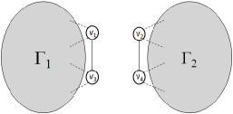
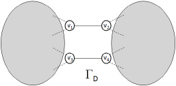
Figure 18: Graphs $\Gamma_{1}$, $\Gamma_{2}$ and $\Gamma_{D}$ as described in Case 1 of Proposition 5.2

Case 2: At least one of the edges $(v_{1},v_{3})$ or $(v_{2},v_{4})$ is present in $\Gamma_{D}$. In this case, the 2-cracker cannot be obtained from a type 2 breeding operation, as such an operation would remove these edges. A 2-cracker of this type is therefore reducible. If both edges are present, we can focus on either one. Without loss of generality, we will assume that edge $(v_{1},v_{3})\in E_{D}$. Then, since $\Gamma_{D}$ is cubic, and vertex $v_{1}$ is adjacent to vertices $v_{2}$ and $v_{3}$, it will be adjacent to one more vertex, say vertex $a$. Similarly, since vertex $v_{3}$ is adjacent to vertices $v_{1}$ and $v_{4}$, it will be adjacent to one more vertex, say vertex $b$. Note that it is possible that $a=b$, so we need to consider the cases separately.

Case 2.1: $a=b$. In this case, edge $(v_{1},a)\in E_{D}$ and edge $(v_{3},a)\in E_{D}$, as illustrated in Figure 19. Since $\Gamma_{D}$ is cubic, vertex $a$ is adjacent to a third vertex, say $c$. Clearly, edge $(a,c)$ is a bridge. Then, we define a cubic graph $\Gamma_{1}=\left<V_{1},E_{1}\right>$, where $V_{1}=V_{D}\backslash\{v_{1},v_{3}\}$ and $E_{1}=E_{D}\backslash\{(v_{1},v_{2}),(v_{3},v_{4}),(v_{1},v_{3}),(a,v_{1}),(a,v_{3})\}\;\cup\;\{(a,v_{2}),(a,v_{4})\}$. Then, we can obtain $\Gamma_{D}$ from the type 3 parthenogenic operation $\mathcal{P}_{3}(\Gamma_{1},a)$. Note that this case is essentially the same as Case 2.2 in Proposition 5.1.

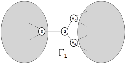
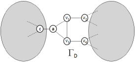
Figure 19: Graphs $\Gamma_{1}$ and $\Gamma_{D}$ as described in Case 2.1 of Proposition 5.2

Case 2.2: $a\neq b$. It is obvious that the non-adjacent edges $(v_{1},a)$ and $(v_{3},b)$ form a cutset. This implies that either both edges are $1$-crackers, or together they form a $2$-cracker. The former situation is covered in Proposition LABEL:prop:graphs_With_1_cracker and $\Gamma_{D}$ can be obtained from either type 1 breeding, type 1 parthenogenesis, or type 3 parthenogenesis. For the latter situation, let us define a cubic graph $\Gamma_{1}=\left<V_{1},E_{1}\right>$, where $V_{1}=V_{D}\backslash\{v_{1},v_{3}\}$ and $E_{1}=E_{D}\backslash\{(v_{1},v_{2}),(v_{3},v_{4}),(v_{1},v_{3}),(a,v_{1}),(b,v_{3})\}\;\cup\;\{(a,v_{2}),(b,v_{4})\}$, as illustrated in Figure 20. We can then obtain $\Gamma_{D}$ from the type 2 parthenogenic operation $\mathcal{P}_{2}(\Gamma_{1},(a,v_{2}),(b,v_{4}))$.    $\Box$

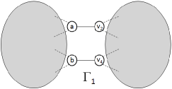
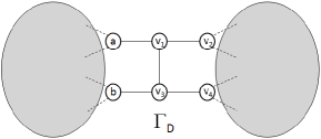
Figure 20: Graphs $\Gamma_{1}$ and $\Gamma_{D}$ as described in Case 2.2 of Proposition 5.2

Proposition 5.3.

Any descendant involving a $3$-cracker can be obtained from type 3 breeding.

Proof.   Consider a descendant $\Gamma_{D}=\left<V_{D},E_{D}\right>$ containing a $3$-cracker comprising edges $(v_{1},v_{2})$, $(v_{3},v_{4})$ and $(v_{5},v_{6})$, as illustrated in Figure 21. Then, suppose the edges $(v_{1},v_{2})$, $(v_{3},v_{4})$ and $(v_{5},v_{6})$ are removed from $\Gamma_{D}$, separating the graph into two subgraphs $\Gamma_{S1}=\left<V_{S1},E_{S1}\right>$ and $\Gamma_{S2}=\left<V_{S2},E_{S2}\right>$. Without loss of generality, we assume that $\{v_{1},v_{3},v_{5}\}\in V_{S1}$ and $\{v_{2},v_{4},v_{6}\}\in V_{S1}$. Then, we introduce a new vertex $v_{7}$, and define a cubic graph $\Gamma_{1}=\left<V_{1},E_{1}\right>$, where $V_{1}=V_{S1}\;\cup\;\{v_{7}\}$ and $E_{1}=E_{S1}\;\cup\;\{(v_{1},v_{7}),(v_{3},v_{7}),(v_{5},v_{7})\}$. Similarly, we introduce a new vertex $v_{8}$, and define a second cubic graph $\Gamma_{2}=\left<V_{2},E_{2}\right>$, where $V_{2}=V_{S2}\;\cup\;\{v_{8}\}$ and $E_{2}=E_{S2}\;\cup\;\{(v_{2},v_{8}),(v_{4},v_{8}),(v_{6},v_{8})\}$. Then, we can obtain $\Gamma_{D}$ from the type 3 breeding operation $\mathcal{B}_{3}(\Gamma_{1},\Gamma_{2},v_{7},v_{8},v_{1},v_{3},v_{5},v_{2},v_{4},v_{6})$.    $\Box$

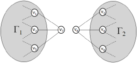
Figure 21: Graphs $\Gamma_{1}$, $\Gamma_{2}$ and $\Gamma_{D}$ as described in Proposition 5.3

Note that any 3-cracker can be obtained from a type 3 breeding operation, and therefore all 3-crackers are irreducible.

Definition 5.4.

We refer to a set of genes that can, through a series of breeding and parthenogenic operations, be used to produce a descendant $\Gamma_{D}$ as ancestor genes for $\Gamma_{D}$.

Propositions 5.1 – 5.3 and Definition 5.4 allow us to derive the main theorem of this section.

Theorem 5.5.

Consider any descendant cubic graph $\Gamma_{D}.$ Then,

1. $\Gamma_{D}$ can be obtained from one or two parents by at least one of the six operations $\mathcal{B}_{1}(\cdot)$, $\mathcal{B}_{2}(\cdot)$, $\mathcal{B}_{3}(\cdot)$, $\mathcal{P}_{1}(\cdot)$, $\mathcal{P}_{2}(\cdot)$, $\mathcal{P}_{3}(\cdot)$.

2. Every descendant $\Gamma_{D}$ has a set of ancestor genes.

Proof.   Any descendant graph contains at least one cubic cracker. Any one of these cubic crackers can be selected, which will be either a 1-cracker, a $2$-cracker, or a $3$-cracker. Then, from Propositions 5.1, 5.2 and 5.3, we can obtain $\Gamma_{D}$, from either one or two parents, using one of the six operations. Therefore (1) is proved.

Next, consider how $\Gamma_{D}$ is obtained. If $\Gamma_{D}$ is obtained through breeding, it has two parent graphs. If $\Gamma_{D}$ is obtained through parthenogenesis, it has one parent graph. These parent graphs may be either genes, or descendants. If any of them are descendants, then by part (1) they also have one or two parent graphs each. Inductively, we can continue to consider the parents of descendants, while recording which operations are used to produce them, thereby obtaining an ancestral family tree of $\Gamma_{D}$. Once the entire tree is determined, all of the top nodes are genes, and we can recall the sequence of operations that produces $\Gamma_{D}$ from these genes. Therefore (2) is proved.    $\Box$

See Figure 22 for an example of an ancestral family tree for a descendant with 14 vertices.

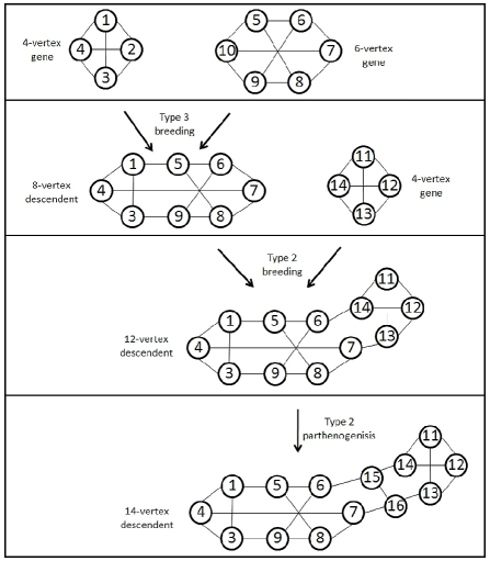
Figure 22: An ancestral family tree for a 14-vertex descendant, with three ancestor genes

Theorem 5.5 indicates that, for any descendant, we can obtain a set of ancestor genes by first applying an inverse operation to obtain one or two parents. Then we can apply an inverse operation on the parent(s) to obtain new parents (grandparents of the original descendant), and continue to apply inverse operations until a set of ancestor genes is obtained.

However, a given descendant may contain only reducible cubic crackers, which do not permit inverse breeding operations. In these cases, inverse parthenogenic operations can be performed, if one of the three parthenogenic objects are present within the descendant. The removal of such a parthenogenic object often changes a reducible cracker into an irreducible cracker which, in turn, permits an inverse breeding operation to be carried out. The following proposition ensures that, for any descendant, at least one of the cubic crackers permits an inverse operation, and furthermore that every reducible cracker in a given descendant can be changed into an irreducible cracker by a sequence of inverse parthenogenic operations.

Proposition 5.6.

If a graph $\Gamma_{D}$ is a descendant, one of the following must be true.

1. $\Gamma_{D}$ contains at least one irreducible cubic cracker, or

2. It is possible to perform a sequence of inverse parthenogenic operations, each time obtaining a new parent, until a parent is obtained that contains at least one irreducible cubic cracker.

Proof.   Since $\Gamma_{D}$ is a descendant, it contains one or more cubic crackers. If any of them are irreducible, then (1) is true. If all the cubic crackers are reducible, then $\Gamma_{D}$ contains at least one $1$-cracker or $2$-cracker (as $3$-crackers are always irreducible). We can therefore select either a reducible $1$-cracker or a reducible $2$-cracker in $\Gamma_{D}$. We will consider both cases separately.

Case 1: We select a reducible $1$-cracker $C_{1}=\{(a,b)\}$. Since $\Gamma_{D}$ is cubic, we know that $a$ must be adjacent to two more vertices, say $c$ and $d$. Since $C_{1}$ is reducible, then without loss of generality, we can assume that edge $(c,d)$ is present in $\Gamma_{D}$. Then, the cubicity of $\Gamma_{D}$ also ensures that vertices $c$ and $d$ must each be adjacent to one more vertex, say $e$ and $f$ respectively. Note that it is possible that $e=f$.

Case 1.1: If $e=f$, then the cubicity of $\Gamma_{D}$ ensures that vertex $e$ must be adjacent to one more vertex, say $g$ (see Figure 23). Then, removing edges $(a,b)$ and $(e,g)$ from $\Gamma_{D}$ disconnects a parthenogenic diamond, which we can remove from $\Gamma_{D}$ by use of the inverse type 1 parthenogenic operation $\mathcal{P}^{-1}_{1}(\Gamma_{D},(a,b),(e,g))$. In the parent graph $\Gamma_{P}$, there is a new $1$-cracker comprising edge $(b,g)$. Note that the new $1$-cracker may also be reducible.

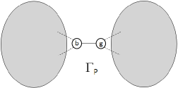
Figure 23: Graphs $\Gamma_{D}$ and $\Gamma_{P}$ as described in Case 1.1

Case 1.2: If $e\neq f$, then removing edges $(a,b)$, $(c,e)$ and $(d,f)$ from $\Gamma_{D}$ isolates a parthenogenic triangle (see Figure 24), which we can remove from $\Gamma_{D}$ by use of the inverse type 3 parthenogenic operation $\mathcal{P}^{-1}_{3}(\Gamma_{D},a,c,d)$. In the parent graph $\Gamma_{P}$, the original $1$-cracker $C_{1}=\{(a,b)\}$ remains. Note that the $1$-cracker may still be reducible.

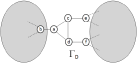
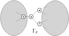
Figure 24: Graphs $\Gamma_{D}$ and $\Gamma_{P}$ as described in Case 1.2

Case 2: We select a reducible $2$-cracker $C_{2}=\{(a,b),(c,d)\}$. Since $C_{2}$ is reducible, then without loss of generality, we can assume that edge $(a,c)$ is present in $\Gamma_{D}$. Then, the cubicity of $\Gamma_{D}$ also ensures that vertices $a$ and $c$ must each be adjacent to one more vertex, say $e$ and $f$, respectively. Note that it is possible that $e=f$.

Case 2.1: If $e=f$, then as illustrated in Figure 25, the cubicity of $\Gamma_{D}$ ensures that vertex $e$ must be adjacent to one more vertex, say $g$. Then, removing edges $(a,b)$, $(c,d)$ and $(e,g)$ from $\Gamma_{D}$ disconnects a parthenogenic triangle, which we can remove from $\Gamma_{D}$ by use of the inverse type 1 parthenogenic operation $\mathcal{P}^{-1}_{1}(\Gamma_{D},a,c)$. In the parent graph $\Gamma_{P}$, a $1$-cracker comprising edge $(e,g)$ remains. Note that this $1$-cracker may still be reducible.

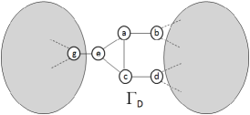
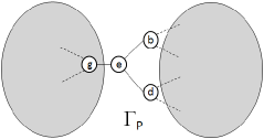
Figure 25: Graphs $\Gamma_{D}$ and $\Gamma_{P}$ as described in Case 2.1

Case 2.2: If $e\neq f$, then as illustrated in Figure 26, the removal of edges $(a,b)$, $(c,d)$, $(a,e)$ and $(c,f)$ from $\Gamma_{D}$ disconnects a parthenogenic bridge, which we can remove from $\Gamma_{D}$ by use of the inverse type 2 parthenogenic operation $\mathcal{P}^{-1}_{2}(\Gamma_{D},a,c)$. In the parent graph $\Gamma_{P}$, there is a new $2$-cracker comprising edges $(e,b)$ and $(f,d)$. Note that this $2$-cracker may be reducible.

Figure 26: Graphs $\Gamma_{D}$ and $\Gamma_{P}$ as described in Case 2.2

Since in all cases considered, the parent graph contains a cubic cracker (either a new one introduced by an inverse parthenogenic operation, or one that remains from the original descendant), the parent is itself always a descendant. Then, either (1) is true for this parent, or if not, we can repeat the above procedure until we obtain a parent for which (1) is true. Since each inverse parthenogenic process outputs a parent with fewer vertices than its child, we are guaranteed to eventually converge to such a case.    $\Box$

6 Conclusions

The theory presented above allows us to separate the set $S$ of connected cubic graphs into two distinct and encompassing categories - the comparatively smaller set of genes, that form the basic building blocks of $S$, and the much larger set of descendants, that inherit a lot of their structure from the genes. Theorem 5.5 and Proposition 5.6 give both a proof of existence, and a guarantee of obtaining a set of ancestor genes for any given descendant. An algorithm to identify a set of ancestor genes, given a descendant, would be a simple task of identifying all the crackers, surveying each until one is found that permits an inverse operation, and recursively repeating the process in each parent obtained until only genes remain. Such an algorithm would terminate in polynomial time.

In addition to the aesthetic beauty of rendering the ancestry of cubic graphs as finite sets of smaller cubic graphs, there are some important algorithmic benefits as well. Since descendants inherit much of their structure from genes, it is possible that a search for graph theoretic properties within a descendant could be more efficiently recast as a search of the (typically much smaller) genes instead. In this context, Theorem 5.5 and Proposition 5.6 give rise to a generic decomposition algorithm that could be applied on most cubic graphs. Since the ancestor genes also lie within the set of connected cubic graphs, any existing algorithms designed for cubic graphs will work for the genes.

For example, experimental evidence indicates that many non-bridge non-Hamiltonian cubic graphs are descendants that contain at least one mutant ancestor gene. In these cases, it is clear that the descendant has inherited the non-Hamiltonicity property from its ancestor mutant gene (or genes). Then, an obvious heuristic for determining Hamiltonicity in a descendant is to identify a set of ancestor genes and determine their Hamiltonicity instead, using whatever state of the art algorithms are available (e.g. see Eppstein [Eppstein 03]). Since determining Hamiltonicity is an NP-complete problem, and therefore the best known algorithms have exponential solving time, such a decomposition represents a large saving in solving time. It is potentially possible that the Hamiltonian cycle problem, already known to be NP-complete even when considering only cubic graphs [Garey and Johnson 79], could be further refined to requiring the consideration of only genes. If so, the extreme rarity of mutants indicates such an avenue could potentially be fruitful. The inheritance of non-Hamiltonicity, and other such graph theoretic properties, is a subject for future research.

Given that properties can be inherited from a set of ancestor genes, a natural question to ask is how many different sets of ancestor genes a descendant graph might have, and how their various (potentially conflicting) properties may influence the single descendant. The following conjecture, if correct, removes any such confusion.

Conjecture 6.1.

Any descendant $\Gamma_{D}$ has a unique set of ancestor genes.

To support Conjecture 6.1, we conducted experiments on individual graphs in which we considered all possible ways to decompose the graph into a set of ancestor genes, and verified that each of these approaches gave the same set of ancestor genes. This experiment was performed on all cubic graphs containing up to 18 vertices, and all triangle-free 20-vertex cubic graphs, constituting 143,528 graphs. For these sizes, there can be up to 7! = 5040 possible ways to decompose a graph into ancestor genes. No counterexample to Conjecture 6.1 was found among the tested graphs.

If Conjecture 6.1 is true it provides, along with Theorem 5.5, a guarantee of existence and uniqueness of ancestor genes for every cubic graph. For such a graph, the above implies that it is either a gene, or there is a unique set of ancestor genes which can be identified in polynomial time, and that these ancestor genes provide the majority of structure in the descendant. If false, Conjecture 6.1 may still be true for all but very special classes of descendants. Note that although the conjecture postulates the existence of a unique set of ancestor genes for any given descendant, the order of breeding operations used to obtain the descendant is clearly not unique.

References

- [Balaban and Harary 71] Balaban, A.T. and Harary, F.: The characteristic polynomial does not uniquely determine the topology of a molecule. J. Chem. Doc. 11, 258–259 (1971)
- [Batagelj 86] Batagelj, V.: Inductive classes of graphs. Proc. Sixth. Yugosl. Semin. Graph Th., Dubrovnik, 1985, 43–56 (1986)
- [Blanus̆a 46] Blanus̆a, D.: Problem cetiriju boja. Glasnik Mat. Fiz. Astr. Ser. II 1, 31–42 (1946)
- [Brinkmann 96] Brinkmann, G.: Fast Generation of Cubic Graphs. J. Graph Th. 23, 139–149 (1996)
- [Ding and Kanno 06] Ding, G. and Kanno, J.: Splitter theorems from cubic graphs. Combin. Probab. Comput. 1̱5, 355–375 (2006)
- [Eppstein 03] Eppstein, D.: The traveling salesman problem for cubic graphs. In: Dehne, F., Sack, J-R., and Smid, M. (eds.) Algorithms and Data Structures, volume 2748 of Lecture Notes in Computer Science, pp. 307–318. Springer, Heidelberg (2003)
- [Filar et al. 10] Filar, J.A., Haythorpe, M. and Nguyen, G.T.: A conjecture on the prevalence of cubic bridge graphs. Discuss. Mat. Graph Th. 30(1), 175–179 (2010)
- [Garey and Johnson 79] Garey, M.R. and Johnson, D.S.: Computers and intractiability: A Guide to the Theory of NP-Completeness. W. H. Freeman (1979)
- [Harary 69] Harary, F.: Graph Theory. Addison-Wesley, Reading, MA (1969)
- [Holton and Sheehan 93] Holton, D.A. and Sheehan, J.: The Petersen Graph. Cambridge University Press, Cambridge (1993)
- [Lou et al. 01] Lou, D., Teng, L. and Wu, X.: A polynomial algorithm for cyclic edge connectivity of cubic graphs. Australas. J. Combin. 24, 247–259 (2001)
- [McKay and Royle 86] McKay, B.D. and Royle, G.F.: Constructing the cubic graphs on up to 20 vertices. Ars Combin. 12A, 129–140 (1986)
- [Meringer 99] Meringer, M.: Fast generation of regular graphs and construction of cages. J. Graph Th. 30, 137–146 (1999)
- [Ore 67] Ore, O.: The Four-Colour Problem. Academic Press, New York (1967)
- [Read and Wilson 98] Read, R.C. and Wilson, R.J.: An Atlas of Graphs. Oxford, England: Oxford University Press, p. 263 (1998)
- [Royle 87] Royle, G.: Constructive enumeration of graphs. PhD thesis, University of Western Australia (1987)