Exact Non-Markovian Master Equation and Dispersive Probing of Non-Markovian Process

Abstract

For a bosonic (fermionic) open system in a bath with many bosons (fermions) modes, we derive the exact non-Markovian master equation in which the memory effect of the bath is reflected in the time dependent decay rates. In this approach, the reduced density operator is constructed from the formal solution of the corresponding Heisenberg equations. As an application of the exact master equation, we study the active probing of non-Markovianity of the quantum dissipation of a single boson mode of electromagnetic (EM) field in a cavity QED system. The non-Markovianity of the bath of the cavity is explicitly reflected by the atomic decoherence factor.

I INTRODUCTION

The open quantum system approach is of much significance due to its various applications in physics, e.g., quantum information, quantum transport, and quantum chemistry, etc. Since a realistic quantum system is inevitably coupled to many degrees of freedom in its environment that leads to decoherence of the systems, a general approach to the open quantum system is needed for its dissipative and dephasing process. The dynamics of an open system is conventionally described with three approaches: effective Hamiltonian eff_Hamiltonian1 ; eff_Hamiltonian2 ; CPSun1995 ; CPSun1998 ; LHYu1994 , quantum master equations Breuer ; master_equaiton , and quantum Langevin equations Langevin_equation ; Louisell . The last two approaches are both based on the modeling with system plus bath, while the first one is phenomenologically given by a time-dependent or non-Hermitian Hamiltonian, which could lead to the dissipative motion equations.

About twenty years ago, Yu and one (C. P. S.) of the authors revealed an intrinsic relation between the effective Hamiltonian and quantum Langevin equation, obtained from the Heisenberg equations LHYu1994 ; CPSun1995 . By discarding the quantum fluctuation for the wide wave packet, they derived the effective Hamiltonian of the system through the formally exact solution for the time-dependent wave function of the total system. However, the resulting effective Hamiltonian ignores the memory effect, which is induced by the back action of the bath with time delay. Therefore, if one wanted to recover the non-Markovian phenomenon with memory effect, the quantum fluctuation of the bath must be taken into account in the above Heisenberg equation based approach. To this end, we need start from the Heisenberg equations of the total system, which can reflect the original role of the bath. In this paper, without any approximation, we derive the exact non-Markovian master equation of the system from the formal solution of the Heisenberg equations. The non-Markovian effect is contained in the time-dependent decay rates in a straightforward way PRB08_WMZ .

It is commonly believed that the Markov process happens when the system-bath coupling is weak. However, with the rapid development of experimental technology, the strong-coupling limit can be reached. The theory of open quantum systems in the strong-coupling regime is required for a proper description of the non-Markovian dynamics. Recently, many works on exact quantum master equations have been done  PRD1992 ; PRA04_TYu ; PRA07_WMZ ; AnnP12_WMZ ; PRB08_WMZ ; NJP10_JSJin ; PRA10_WMZ ; PRA10_Breuer ; HFL . In particular, one (W. M. Z.) of the authors and his collaborators derived the exact non-Markovian master equations with a Lindblad-form for both Bose PRA07_WMZ ; AnnP12_WMZ and Fermi PRB08_WMZ ; NJP10_JSJin systems by a path-integral method in coherent-state representation. We now revisit these non-Markovian master equations by generalizing our previous approach CPSun1998 , which was used to derive a partially factorized wave function for open quantum system. Using the present generalization to derive the reduced density matrix is quite straightforward. Here, we first construct the total density matrix with the help of the formal solution of the Heisenberg equations, and then trace over the degrees of freedom of the bath to obtain the reduced density matrix of the system in the coherent state representation, instead of using the Feynman-Vernon influence functional, as was done in Refs. PRB08_WMZ ; NJP10_JSJin ; AnnP12_WMZ . It reproduces the same reduced density matrix that satisfies a time-local master equation where the non-Markovian memory effect is fully taken into account.

With the help of the exact reduced density matrix, the dynamics of an open quantum system could be well described. Meanwhile, there are several proposals to measure the degree of the non-Markovianity of open quantum process PRL09_Breuer ; PRA10_Sun . Very recently, the general non-Markovian dynamics of the environment on its surrounding open quantum system are explored within the exact master equation arXiv12_WMZhang . The question is how to probe the general non-Markovian dynamics. We thereby propose in this paper a promising approach to probe the time-dependent memory effect of a bath on a damped micro-cavity by coupling the cavity to a two-level atom dispersively. To probe the non-Markovianity of the dissipation of the single model EM field in a cavity, we let atoms of large detuning pass through the cavity. We found that the non-Markovianity of the bath is explicitly reflected by the atomic decoherence factor. In the week coupling region, the periodically reviving amplitude decreases along with the cavity-bath coupling strength and decays to $0$ finally. On the the contrary, in the strong coupling region, the reviving amplitude increases with the coupling strength and almost does not decay in the ultra-strong coupling case, as a significant non-Markovian effect arXiv12_WMZhang . This atomic decoherence factor could be detected through the Ramsey interference in experiments.

In the next section, we solve the Heisenberg equations of the unified quantum system plus bath model (Bose and Fermi) and obtain their formal solutions. In Sec. III, the derivation of the exact master equation of Bose system is presented. The exact master equation of Fermi case is addressed in Sec. IV. In Sec. V, we propose to probe the non-Markovian dynamics of a damped cavity with largely detuned two-level atoms. Finally, the summery of our main results is given in Sec. VI. Some detailed calculations are displayed in the Appendices.

II UNIFIED QUANTUM BATH MODEL AND FORMAL SOLUTION OF THE HEISENBERG EQUATIONS

We consider an open quantum system $S$, which interacts with another large system $B$ called bath. The combined system $S+B$ is usually assumed to be closed, thus regarded as a Universe. The coupling of $S$ to $B$ will lead to the dissipation and dephasing of $S$. There are various types of bath, but the most commonly employed baths are modeled with non-interacting bosons and fermions. In this paper we consider the specific cases: a Bose system is surrounded by a Bose bath, or a Fermi system is immersed in a Fermi bath. Here, we first solve the Heisenberg equations for both the Bose and Fermi cases and obtain their formally exact solutions.

The Universe Hamiltonian $H=H_{s}+H_{b}+H_{\mathrm{int}}$ is decomposed into three parts: the Hamiltonian of the system is taken to be a quadratic form

$$H_{s}=\left[a_{1}^{\dagger},a_{2}^{\dagger},\cdots,a_{N_{s}}^{\dagger}\right]M\left[a_{1},a_{2},\dots,a_{N_{s}}\right]^{T},$$ (1)

which describes $N_{s}$ linearly coupled bosons or fermions. $a_{i}(a_{i}^{\dagger})$ is the annihilation (creation) operator of the $i$th mode of the system satisfying the commutation relation $\left[a_{i},a_{i^{\prime}}^{\dagger}\right]_{\mp}=\delta_{ii^{\prime}}$ ($\mp$ corresponds to the boson and fermion, respectively) and $M$ is a positive definite Hermitian matrix. The Hamiltonian of the Bose or Fermi bath is given by

$$H_{b}=\sum_{l=1}^{N_{b}}\omega_{l}b_{l}^{\dagger}b_{l},$$ (2)

with the number of the uncoupled modes of the bath $N_{b}(\gg N_{s})$ and annihilation (creation) operators $b_{l}$ ($b_{l}^{\dagger}$) which satisfy corresponding commutation relations $\left[b_{l},b_{l^{\prime}}^{\dagger}\right]_{\mp}=$$\delta_{ll^{\prime}}$. As proofed in master_equaiton , the most usual environment coupled to the open system could be well approximated as a collection of harmonic oscillators with linear quadratic couplings. Here, the interaction Hamiltonian is taken as the form of

$$H_{\mathrm{int}}=\sum_{i=1}^{N_{s}}\sum_{l=1}^{N_{b}}\left(\eta_{il}a_{i}^{\dagger}b_{l}+\eta_{il}^{*}b_{l}^{\dagger}a_{i}\right).$$ (3)

In the Heisenberg picture, the dynamics of the system is governed by the Heisenberg equations:

$$\dot{a}_{i}\left(t\right) = -\mathrm{i}\sum_{j}M_{ij}a_{j}\left(t\right)-\mathrm{i}\sum_{l}\eta_{il}b_{l}\left(t\right),$$ (4)

$$\dot{b}_{l}\left(t\right) = -\mathrm{i}\omega_{l}b_{l}\left(t\right)-\mathrm{i}\sum_{i}\eta_{li}^{*}a_{i}\left(t\right).$$ (5)

For convenience, we introduce the $\left(N_{s}+N_{b}\right)$ operator-valued vector

$$\vec{c}\left(t\right)\!\!=\!\!\left[\!\vec{a},\vec{b}\right]^{T}\!\!\!\!=\!\!\left[a_{1}\!\!\left(\!t\!\right)\!,a_{2}\!\!\left(\!t\!\right)\!,\!\cdots\!,a_{N_{s}}\!\!\left(\!t\!\right)\!,b_{1}\!\!\left(\!t\!\right)\!,b_{2}\!\!\left(\!t\!\right)\!,\!\cdots\!,b_{N_{b}}\!\!\left(\!t\!\right)\right]^{T}\!\!\!\!\!,$$

and the $\left(N_{s}+N_{b}\right)\times\left(N_{s}+N_{b}\right)$ coefficient matrix

$$\mathcal{H}=\left[\begin{array}[]{cc}M&R\\ R^{\dagger}&E\end{array}\right],$$ (6)

where

$$R=\left[\begin{array}[]{cccc}\eta_{11}&\eta_{12}&\dots&\eta_{1N_{b}}\\ \eta_{21}&\eta_{22}&\cdots&\eta_{2N_{b}}\\ \vdots&\vdots&\vdots&\vdots\\ \eta_{N_{s}1}&\eta_{N_{s}2}&\cdots&\eta_{N_{s}N_{b}}\end{array}\right],$$

and

$$E=\mathrm{diag}\left[\omega_{1},\omega_{2},\cdots,\omega_{N_{b}}\right].$$

Then Eqs. (4) and (5) are re-expressed in a compact form

$$\frac{d}{dt}\vec{c}\left(t\right)=-\mathrm{i}\mathcal{H}\vec{c}\left(t\right).$$ (7)

It follows from Eq. (6) that $\mathcal{H}$ is a time-independent Hermitian matrix. Consequently, the formal solution of Eq. (7) is given by

$$\vec{c}\left(t\right)=\exp\left[-\mathrm{i}\mathcal{H}t\right]\vec{c}\left(0\right)\equiv\mathcal{U}\left(t\right)\vec{c}\left(0\right),$$

where $\mathcal{U}\left(t\right)=\exp\left[-\mathrm{i}\mathcal{H}t\right]$ is the time-evolution operator. Splitting the matrix $\mathcal{U}\left(t\right)$ into four blocks

$$\mathcal{U}\left(t\right)\equiv\left[\begin{array}[]{cc}\left[W\left(t\right)\right]_{N_{s}\times N_{s}}&\left[T\left(t\right)\right]_{N_{s}\times N_{b}}\\ \left[P\left(t\right)\right]_{N_{b}\times N_{s}}&\left[Q\left(t\right)\right]_{N_{b}\times N_{b}}\end{array}\right],$$ (8)

we obtain formal solution of Eq. (7) as

$$\vec{a}\left(t\right) = W\left(t\right)\vec{a}\left(0\right)+T\left(t\right)\vec{b}\left(0\right),$$ (9)

$$\vec{b}\left(t\right) = P\left(t\right)\vec{a}\left(0\right)+Q\left(t\right)\vec{b}\left(0\right).$$ (10)

The dynamics of total system is governed by these four time-dependent coefficient matrices $W\left(t\right)$, $T\left(t\right)$, $Q\left(t\right)$, and $P\left(t\right)$.

Up to now, all the results are obtained by formal operations, since these coefficient matrices need to be determined by the differential equations. As shown in Appendix B, there are some connections between these coefficient matrices, which take a crucial role in derivation of the exact master equation.

II.1 Differential equations of the coefficient matrices

Substituting Eqs. (9) and (10) into Eqs. (4) and (5), we obtain the equations of the coefficient matrices

$$\dot{W}\left(t\right) = -\mathrm{i}\left[MW\left(t\right)+RP\left(t\right)\right],$$ (11)

$$\dot{T}\left(t\right) = -\mathrm{i}\left[MT\left(t\right)+RQ\left(t\right)\right],$$ (12)

$$\dot{P}\left(t\right) = -\mathrm{i}\left[EP\left(t\right)+R^{\dagger}W\left(t\right)\right],$$ (13)

$$\dot{Q}\left(t\right) = -i\left[EQ\left(t\right)+R^{\dagger}T\left(t\right)\right],$$ (14)

with the initial conditions

$$W\left(0\right)=I,\ T\left(0\right)=\mathbf{0},\ P\left(0\right)=\mathbf{0},\ Q\left(0\right)=I.$$ (15)

Here, $I$ is the identity matrix and $\mathbf{0}$ is the null matrix. The differential equations of $P\left(t\right)$ and $Q\left(t\right)$ are integrated to yield

$$P\left(t\right) = -\mathrm{i}\int_{0}^{t}d\tau e^{-\mathrm{i}E\left(t-\tau\right)}R^{\dagger}W\left(\tau\right)d\tau,$$ (16)

$$Q\left(t\right) = e^{-\mathrm{i}Et}\left[-\mathrm{i}\int_{0}^{t}d\tau e^{\mathrm{i}E\tau}R^{\dagger}T\left(\tau\right)+I\right].$$ (17)

Then, we obtain the integrodifferential equations about $W\left(t\right)$ and $T\left(t\right)$:

$$\dot{W}\left(t\right)+\mathrm{i}MW\left(t\right)+\int_{0}^{t}d\tau G\left(t-\tau\right)W\left(\tau\right) = 0,$$ (18)

$$\dot{T}\left(t\right)+\mathrm{i}MT\left(t\right)+\int_{0}^{t}d\tau G\left(t-\tau\right)T\left(\tau\right)=-\mathrm{i}Re^{-\mathrm{i}Et}\!.$$ (19)

Here the ($N_{s}\times N_{s}$) kernel matrix $G\left(t\right)=Re^{-\mathrm{i}Et}R^{\dagger}$ characterizes the non-Markovian memory structure of $S$. Defining the interaction spectral function

$$J_{ij}\left(\omega\right)=\sum_{l}\eta_{il}\eta_{lj}^{*}\delta\left(\omega-\omega_{l}\right),$$

we rewrite the element of the kernel matrix $G\left(t\right)$ as

$$G_{ij}\left(t\right)=\int d\omega J_{ij}\left(\omega\right)e^{-i\omega t}.$$

Thus, the matrix $G\left(t\right)$ is fully determined by the interaction spectrum.

On the other hand, the coefficient matrices $W\left(t\right)$ and $T\left(t\right)$ are not independent. By taking the Laplace transform of the integral differential equations (18) and (19), we get

$$W[p] = \mathcal{L}\left(W\right)=\left[p+\mathrm{i}M+G\left(p\right)\right]^{-1},$$ (20)

$$T[p] = W[p]\mathcal{L}\left(-\mathrm{i}Re^{-\mathrm{i}Et}\right),$$ (21)

where $\mathcal{L}\left(\cdots\right)$ represents the Laplace transform. Consequently, after the inverse Laplace transform, the matrix $T\left(t\right)$ is given by

$$T\left(t\right)=-\mathrm{i}\int_{0}^{t}d\tau W\left(t-\tau\right)Re^{-\mathrm{i}E\tau}.$$ (22)

Thus the dynamics of $S$ could be completely described by a single coefficient matrix $W\left(t\right)$, It is well known that, under the Wigner-Weisskopff approximation, one can obtain the quantum Langevin equations of the operators of $S$ by means of the approximate solution of Eqs.(18) and (19) together with the Heisenberg equations (4) and (5) Louisell . In this paper, it will be shown that the exact master equation of the reduced density matrix can also be obtained based on the formal solutions (9-10) of the Heisenberg equations. And the Wigner-Weisskopff approximation leads to the quantum Born-Markov master equation.

III BOSON CASE IN COHERENT-STATE REPRESENTATION

In this section, we derive the exact master equation for $N_{s}$ coupled bosons in a Bose bath. In the Schr$\ddot{\mathrm{o}}$dinger picture, the total density matrix $\rho\left(t\right)=U\left(t\right)\rho\left(0\right)U^{\dagger}\left(t\right)$ of $S+B$ obeys the Liouville-von Neumann equation $\mathrm{i}\hbar\dot{\rho}\left(t\right)=\left[H,\rho\left(t\right)\right]$, where $U\left(t\right)=\exp\left(-\mathrm{i}Ht\right)$ is the time evolution operator of the total system. We assume that the total system is initially in the direct product initial state $\rho\left(0\right)=\rho_{s}\left(0\right)\otimes\rho_{b}\left(0\right)$, with density matrices $\rho_{s}\left(0\right)$ and $\rho_{b}\left(0\right)$ of $S$ and $B$, respectively. Through a lengthy calculation in Appendix C, the reduced density matrix of $S$ is expressed in terms of the coherent state $\left|\vec{x}\right\rangle$ of the system

$$\rho_{s}\left(t\right) = \int d\mu\left(\vec{\alpha},\vec{\alpha}^{\prime}\right)d\mu\left(\vec{\xi},\vec{\xi}^{\prime}\right)\left|\vec{\alpha}\right\rangle\!\left\langle\vec{\alpha}^{\prime}\right|$$ (23)

$$K\left(\vec{\alpha}^{\dagger},\vec{\alpha}^{\prime},\vec{\xi},\vec{\xi}^{\prime\dagger},t\right)\left\langle\vec{\xi}\right|\rho_{s}\left(0\right)\left|\vec{\xi}^{\prime}\right\rangle,$$

with $\vec{x}=\left[x_{1},x_{2},\cdots,x_{N_{s}}\right]^{T}$ ($\vec{x}=\vec{\alpha},\vec{\alpha}^{\prime},\vec{\xi},\vec{\xi}^{\prime}$). The propagator, which governs the dynamics of the reduced density matrix, is defined as

$$K\left(\vec{\alpha}^{\dagger},\vec{\alpha}^{\prime},\vec{\xi},\vec{\xi}^{\prime\dagger};t\right) = \int d\mu\left(\vec{z}\right)\left\langle\vec{\alpha},\vec{z}\right|U\left(t\right)\left|\vec{\xi}\right\rangle$$ (24)

$$\!\times\!\left\langle\vec{\xi}^{\prime}\right|\rho_{b}\left(0\right)U^{\dagger}\left(t\right)\left|\vec{\alpha}^{\prime},\vec{z}\right\rangle.$$

Here $\left|\vec{z}\right\rangle$$\left(\vec{z}=\left[z_{1},z_{2},\cdots,z_{N_{b}}\right]\right)$ is the coherent state of $B$. Different from the previous derivation PRB08_WMZ ; NJP10_JSJin ; AnnP12_WMZ where the propagating function is obtained using the coherent-state path integral method and tracing over the environmental degrees of freedom completely through the Feynman-Vernon influence functional, the propagator could also be evaluated in the coherent state representation by constructing the explicit total wave function CPSun1998

$$U^{\dagger}\left(t\right)\left|\vec{\alpha}^{\prime},\vec{z}\right\rangle=\exp\left[\vec{a}^{\dagger}\left(t\right)\cdot\vec{\alpha}^{\prime}+\vec{b}^{\dagger}\left(t\right)\cdot\vec{z}\right]\left|0\right\rangle,$$ (25)

as shown in Appendix C. It deserves to be noted that we have used the identities $U^{\dagger}\left(t\right)\left|0\right\rangle=\left|0\right\rangle$ and $O\left(t\right)=U^{\dagger}\left(t\right)OU\left(t\right)$.

III.1 Propagating Function

Generally speaking, the bath is initially in its thermal equilibrium state

$$\rho_{b}\left(0\right)=\left(\prod_{l}\frac{1}{f_{l}+1}\right)\exp\left[-\beta\vec{b}^{\dagger}E\vec{b}\right],$$ (26)

where $f_{l}=1/\left[\exp\left(\beta\omega_{l}\right)-1\right]$ is the mean occupation number of the $l$th bath mode at temperature $T=1/(k_{B}\beta)$. In this case, the integral over the bath in the propagator (24) is carried out to give (please refer to Appendix C for the detail),

$$\!\!\!\!\!\!\!\!\!\!\!\!\!K(\vec{\alpha}^{\dagger},\vec{\alpha}^{\prime},\vec{\xi},\vec{\xi}^{\prime\dagger},t)\! = \!A(t)\!\exp\!\!\left[\!\!\begin{array}[]{c}\vec{\alpha}^{\dagger}J_{1}(t)\vec{\xi}+\vec{\xi}^{\prime\dagger}J_{1}^{\dagger}(t)\vec{\alpha}^{\prime}\\ +\vec{\alpha}^{\dagger}J_{2}(t)\vec{\alpha}^{\prime}+\vec{\xi}^{\prime\dagger}J_{3}\vec{\xi}\!\!\!\!\end{array}\right]\!,$$ (29)

where

$$A\left(t\right)=\mathrm{det}\left[[I+V\left(t\right)]^{-1}\right],$$

$$J_{1}\left(t\right)=[I+V\left(t\right)]^{-1}W\left(t\right),$$

$$J_{2}\left(t\right)=V[I+V\left(t\right)]^{-1},$$

$$J_{3}\left(t\right)=I-W^{\dagger}\left(t\right)[I+V\left(t\right)]^{-1}W\left(t\right).$$

This reproduces the propagating function obtained by the coherent state path-integral method in the previous works, e.g., Eq. (31) in AnnP12_WMZ . For convenience, we have introduced a new $N_{s}\times N_{s}$ Hermitian matrix $V\left(t\right)=T\left(t\right)fT^{\dagger}\left(t\right)$. Utilizing the relationship in Eq. (22) between the matrices $T\left(t\right)$ and $W\left(t\right)$, we have

$$V\left(t\right)=\int_{0}^{t}d\tau_{1}\int_{0}^{t}d\tau_{2}W\left(\tau_{1}\right)\tilde{G}\left(\tau_{2}-\tau_{1}\right)W^{\dagger}\left(\tau_{2}\right),$$ (30)

with

$$\tilde{G}\left(t\right)=Rfe^{-\mathrm{i}Et}R^{\dagger}.$$ (31)

Without any additional hypothesis, the exact propagating function of the reduced density matrix of $S$ is obtained. The dynamics of $S$ is governed by the single coefficient matrix $W\left(t\right)$, which is determined by integral differential equation (18). And the influence of the bath on the dynamics of $S$ is characterized by two memory-kernel matrices $G\left(t\right)$ and $\tilde{G}\left(t\right)$ PRB08_WMZ ; NJP10_JSJin ; AnnP12_WMZ .

III.2 The Exact Non-Markovian Master equation for Bosons

In the proceeding subsection, we have obtained the exact reduced density matrix of $S$ as in Eq. (23). Now we construct the master equation through its time derivative

$$\dot{\rho}_{s} = \int d\mu\left(\vec{\alpha},\vec{\alpha}^{\prime}\right)d\mu\left(\vec{\xi},\!\vec{\xi}^{\prime}\right)\left|\vec{\alpha}\right\rangle\left\langle\vec{\alpha}^{\prime}\right|$$ (32)

$$\dot{K}\!\!\left(\!\vec{\alpha}^{\dagger},\vec{\alpha}^{\prime},\vec{\xi},\vec{\xi}^{\prime\dagger};t\right)\left\langle\vec{\xi}\right|\rho_{s}\left(0\right)\left|\vec{\xi}^{\prime}\right\rangle.$$

And it is found that the time differential of the propagating function takes the following form (please refer to Appendix D for the detail)

$$\!\!\!\dot{K} = \vec{\alpha}^{\dagger}\tilde{\Gamma}K\vec{\alpha}^{\prime}-\mathrm{Tr}\left[\tilde{\Gamma}\right]K-\vec{\alpha}^{\dagger}\left(\Gamma+\mathrm{i}\tilde{\Omega}+\tilde{\Gamma}\right)\overset{\rightarrow}{\nabla}_{\alpha^{*}}K$$ (33)

$$\!\!\!\!-\!\left(\!\overset{\rightarrow}{\nabla}_{\alpha^{\prime}}^{T}\!K\right)\!\left(\Gamma\!-\!\mathrm{i}\tilde{\Omega}\!+\!\tilde{\Gamma}\right)\!\vec{\alpha}^{\prime}\!+\!\overset{\rightarrow}{\nabla}_{\alpha^{\prime}}^{T}\!\left(\tilde{\Gamma}\!+\!2\Gamma\right)\!\!\overset{\rightarrow}{\nabla}_{\alpha^{*}}K,$$

with Hermitian matrices

$$\tilde{\Gamma}\left(t\right)=\dot{V}\left(t\right)-\dot{W}\left(t\right)W^{-1}\left(t\right)V\left(t\right)-V\left(\dot{W}\left(t\right)W^{-1}\left(t\right)\right)^{\dagger},$$ (34)

$$\Gamma\left(t\right)=-\frac{1}{2}\left[\dot{W}\left(t\right)W^{-1}\left(t\right)+\left(\dot{W}\left(t\right)W^{-1}\left(t\right)\right)^{\dagger}\right],$$ (35)

and

$$\tilde{\Omega}\left(t\right)=\frac{\mathrm{i}}{2}\left[\dot{W}\left(t\right)W^{-1}\left(t\right)-\left(\dot{W}\left(t\right)W^{-1}\left(t\right)\right)^{\dagger}\right].$$ (36)

For coherent state defined in Eq. (53), there exist the following relations PRA1994_correspondence

$$\vec{\alpha}\left|\vec{\alpha}\right\rangle = \vec{a}\left|\vec{\alpha}\right\rangle,\ \vec{\alpha}^{\dagger}\left\langle\vec{\alpha}\right|=\left\langle\vec{\alpha}\right|\vec{a}^{\dagger},$$

$$\overset{\rightarrow}{\nabla}_{\alpha}^{T}\left|\alpha\right\rangle = \vec{a}^{\dagger}\left|\vec{\alpha}\right\rangle,\ \overset{\rightarrow}{\nabla}_{\alpha^{*}}\left\langle\vec{\alpha}\right|=\left\langle\vec{\alpha}\right|\vec{a}.$$

With these mapping, we can construct the exact master equation of the reduced density matrix of the Bose system $S$, i.e. Eq. (32) in Ref. AnnP12_WMZ ,

$$\dot{\rho}_{s}\left(t\right)\! = -\mathrm{i}\left[\tilde{H}_{s}\left(t\right),\rho_{s}\left(t\right)\right]+\sum_{ij}\left[\tilde{\Gamma}_{ij}\left(t\right)+2\Gamma_{ij}\left(t\right)\right]\left[a_{j}\rho_{s}\left(t\right)a_{i}^{\dagger}-\frac{1}{2}a_{i}^{\dagger}a_{j}\rho_{s}\left(t\right)-\frac{1}{2}\rho_{s}a_{i}^{\dagger}a_{j}\right]$$ (37)

$$+\sum_{ij}\tilde{\Gamma}_{ij}\left(t\right)\left[a_{i}^{\dagger}\rho_{s}\left(t\right)a_{j}-\frac{1}{2}a_{j}a_{i}^{\dagger}\rho_{s}\left(t\right)-\frac{1}{2}\rho_{s}\left(t\right)a_{j}a_{i}^{\dagger}\right],$$

where $\tilde{H}_{s}=\vec{a}^{\dagger}\tilde{\Omega}\vec{a}$ is the effective time-dependent Hamiltonian of the system $S$. The diagonal elements of $\tilde{\Omega}\left(t\right)$ are the modified time-dependent frequencies of the different modes of $S$ and the off-diagonals represent the new interaction strength between the modes of the system. Without Markov approximation, the dissipation of the system and the fluctuation of the bath could not be separated. The original role of the bath is reflected by the time-dependent decay coefficients $\Gamma\left(t\right)$ and $\tilde{\Gamma}\left(t\right)$ AnnP12_WMZ .

III.3 From Wigner-Weisskopff Approximation to Markov Master Equation

In this subsection, it will be shown that the Markov master equation can be obtained from the exact master equation by taking Wiger-Weisskopff approximation Louisell , instead of making a direct Markov approximation PRA10_WMZ . Here the exact master equation is applied to the simplest dissipative system consisting of a single harmonic oscillator with frequency $\Omega_{0}$ and a Bose environment. In this case, $\tilde{\Omega}$, $\Gamma\left(t\right)$, and $\tilde{\Gamma}\left(t\right)$ are just time-dependent numbers instead of matrices, which are all determined by $W\left(t\right)$ in Eqs. (34-36). Under the Wigner-Weisskopff approximation, the solution of Eq. (18) is given by

$$W(t)=\exp\left[-\Gamma_{0}t-i(\Omega_{0}+\Delta\omega)t\right],$$ (38)

where

$$\Gamma_{0}=\pi J\left(\Omega_{0}\right),$$ (39)

is the decay rate of the oscillator induced by the coupling to the vacuum and

$$\Delta\omega=-\mathcal{P}\int\frac{J\left(\Omega_{0}\right)}{\omega-\Omega_{0}}d\omega,$$ (40)

is the small frequency shift, with the interaction spectrum $J\left(\omega\right)$. It is easy to find that, in this case, the parameters of the master equation become time-independent

$$\tilde{\Omega}=\Omega_{0}+\Delta\omega,\ \Gamma=\Gamma_{0},\ \tilde{\Gamma}=2f\left(\Omega_{0}\right)\gamma_{0},$$ (41)

where $f\left(\Omega_{0}\right)$ is the mean occupation number of the oscillator. As we know, $\Gamma$ characterizes the dissipation of the system and $\tilde{\Gamma}$ corresponds to the fluctuation of the bath.

Then the Born-Markov master equation of a damped harmonic resonator is obtained as

$$\dot{\rho}_{s}(t)= -i[\tilde{\Omega}a^{\dagger}a,\rho_{s}(t)]+\left[1+f(\Omega_{0})\right]\Gamma_{0}\left[2a\rho_{s}(t)a^{\dagger}-\left(a^{\dagger}a\rho_{s}(t)+\rho_{s}(t)a^{\dagger}a\right)\right]$$

$$+f(\Omega_{0})\Gamma_{0}\left[2a^{\dagger}\rho_{s}(t)a-\left(aa^{\dagger}\rho_{s}(t)-\rho_{s}(t)aa^{\dagger}\right)\right].$$ (42)

It is known that, for a damped harmonic oscillator, the quantum Langevin equation of the number operator obtained from the Markov approximation is same as the one from the Wigner-Weisskopff approximation Louisell . In this sense, these two approximations are equivalent.

IV FERMI CASE IN COHERENT STATE REPRESENTATION

In the previous section, we obtained the exact master equation of the Bose system. Analogously, in the case of Fermi system, the reduced density matrix in the fermion coherent state representation fermion_coherent1 ; fermion_coherent2 reads

$$\rho_{s}\left(t\right) = \int d\mu\left(\vec{\alpha},\vec{\alpha}^{\prime}\right)d\mu\left(\vec{\xi},\vec{\xi}^{\prime}\right)\left|\vec{\alpha}\right\rangle\left\langle\vec{\alpha}^{\prime}\right|$$ (43)

$$\times K\left(\vec{\alpha}^{\dagger},\vec{\alpha}^{\prime},\vec{\xi},\vec{\xi}^{\prime\dagger},t\right)\left\langle\vec{\xi}\right|\rho_{s}\left(0\right)\left|\vec{\xi}^{\prime}\right\rangle,$$

where the components of vectors $\vec{\alpha}$, $\vec{\alpha}^{\prime}$, $\vec{\xi}$, and $\vec{\xi}^{\prime}$ are Grassmann variables, $\rho_{s}\left(0\right)$ is the initial state of $S$. And the initial state of the bath is still assumed to be the thermal state

$$\rho_{b}\left(0\right)=\prod_{l}\left(1-f_{l}\right)\exp\left[-\beta\vec{b}^{\dagger}E\vec{b}\right].$$ (44)

where $f_{k}=1/\left[\exp\left(\beta\omega_{l}\right)+1\right]$ is the mean occupation number of the $l$th Fermi mode with $\beta=1/\left(k_{B}T\right)$. After tracing over the degrees of freedom of the bath, we find that the propagator is of the same form as the Bose case PRB08_WMZ ,

$$K=A\exp\left[\vec{\alpha}^{\dagger}J_{1}\vec{\xi}+\vec{\xi}^{\prime}J_{1}^{\dagger}\vec{\alpha}^{\prime}+\vec{\alpha}J_{2}\vec{\alpha}^{\prime}+\vec{\xi}^{\prime\dagger}J_{3}\vec{\xi}\right],$$

but the matrices in $K$ change into

$$A\left(t\right)=\mathrm{det}\left[[I-V\left(t\right)]^{-1}\right],$$

$$J_{1}\left(t\right)=\left[I-V\left(t\right)\right]^{-1}W\left(t\right),$$

$$J_{2}\left(t\right)=\left[I-V\left(t\right)\right]^{-1}-I,$$

$$J_{3}\left(t\right)=W^{\dagger}\left(t\right)\left[I-V\left(t\right)\right]^{-1}W\left(t\right)-I.$$

After the same procedure as the Bose system, the exact master equation of the Fermi system is obtained as the same one given by Eq. (8) in NJP10_JSJin

$$\dot{\rho}_{s}\left(t\right) = -\mathrm{i}\left[\tilde{H}_{s}\left(t\right),\rho_{s}\left(t\right)\right]+\sum_{ij}\left[2\Gamma_{ij}\left(t\right)-\tilde{\Gamma}_{ij}\left(t\right)\right]\left[a_{j}\rho_{s}\left(t\right)a_{i}^{\dagger}-\frac{1}{2}a_{i}^{\dagger}a_{j}\rho_{s}\left(t\right)-\frac{1}{2}\rho_{s}\left(t\right)a_{i}^{\dagger}a_{j}\right]$$ (45)

$$+\sum_{ij}\tilde{\Gamma}_{ij}\left(t\right)\left[a_{i}^{\dagger}\rho_{s}\left(t\right)a_{j}-\frac{1}{2}a_{j}a_{i}^{\dagger}\rho_{s}\left(t\right)-\frac{1}{2}\rho_{s}\left(t\right)a_{j}a_{i}^{\dagger}\right],$$

where $\tilde{H}_{s}\left(t\right)$, $\Gamma\left(t\right)$, and $\tilde{\Gamma}\left(t\right)$ are defined in the same way as the bosons’ PRB08_WMZ ; NJP10_JSJin .

V PROBING NON-MARKOVIANIANITY OF AN OPEN QUANTUM SYSTEM

In this section, we consider how to probe the non-Markovianity of a quantum dissipation process in a realistic physical system. We understand that such an ideal probing scheme is usually based on the non-demolition measurementQuantum_Measurement . The interaction between the probing apparatus and the system to be detected commutes with the free Hamiltonian of the system, thus such kind of measurement does not change the energy of the system. But it will retain the information of the system on the probing apparatus. Such non-demolition interaction can be implemented in the cavity-QED as the dispersive interaction between the atom and cavity PRL90_QND ; PRA92_QND . On the other hand, it is feasible to prepare and analyze a two-level Rydberg atom in a state corresponding to an arbitrary point on the Bloch sphere in the quantum optics experiments.

To realize the probing non-Markovianity in the cavity QED system, we consider an open quantum system: a single cavity mode coupled to its bath of many bosonic excitation modes resulting from the cavity leakage. Let an atom pass through the cavity, and then examine the quantum coherence of the atom. In this case, the atom could record the intrinsic information of the cavity field to accomplish the probing of the non-Markovianity of the cavity dynamics. This kind of approach was also used to probe the quantum criticality of many body system PRL06_HTQuan , where the sensitive change of the atom decoherence factor, which is characterized by the Loschmidt echo Lochsmidt , could reflect the quantum criticality of its surrounding environment.

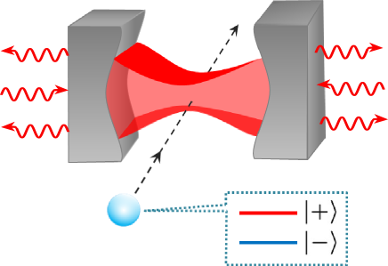
Figure 1: (Color online) Schematic diagram for probing of the non-Markovian dynamics of an open quantum system: a leaking cavity. The two-level atom passing through the cavity is largely detuned from the frequency of the cavity mode to approach the non-demolition measurement.

In our case, the frequency of the atom $\omega_{a}$ is drastically detuned from the the cavity resonance frequency $\omega_{0}$, i.e., $\Delta=\omega_{0}-\omega_{a}\gg g_{a-f}$, where $g_{a-f}$ is the vacuum Rabi frequency characterizing the atom-cavity coupling. By making use of an adiabatic elimination procedure, we obtain the effective Hamiltonian

$$H_{p}=\hbar\omega_{0}a^{\dagger}a+\hbar\omega_{a}\sigma_{z}+\hbar\delta a^{\dagger}a\sigma_{z},$$ (46)

for our probing scheme from the usual Jaynes-Cummings model Scully . Here, $a(a^{\dagger})$ is the annihilation (creation) operator of the cavity, $\sigma_{z}=\left|e\right\rangle\left\langle e\right|-\left|g\right\rangle\left\langle g\right|$ is the Pauli matrix of the atom with the ground (excited) state of the atom $\left|g\right\rangle(\left|e\right\rangle)$, and $\delta=g_{a-f}^{2}/\Delta$ is the effective dispersive coupling constant PRL1996_Haroche ; PRL1997_Haroche . Meanwhile, the cavity is coupled to a bosonic bath

$$H_{b}+H_{\mathrm{int}}=\sum_{l}\hbar\omega_{l}b_{l}^{\dagger}b_{l}+\hbar\sum_{l}\left(\eta_{l}a^{\dagger}b_{l}+\mathrm{H.c.}\right).$$

Here, the atom has enough long coherence time and we neglect the decay of the atom during the strong probing process.

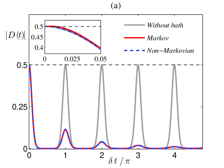
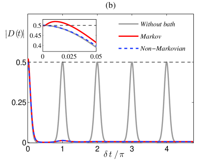
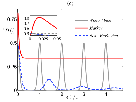
Figure 2: (Color online) Decoherence factor with different cavity-bath coupling strength. ($a$) $\lambda=0.002$. ($b$) $\lambda=0.01$. ($c$) $\lambda=0.1$.

Before entering the cavity, the atom is initialized in the superposition state $\left(\left|e\right\rangle+\left|g\right\rangle\right)/\sqrt{2}$ and the cavity is initially in the coherent state $\left|\alpha\right\rangle$. For simplicity, we assume that the bath is at zero temperature with initial density matrix $\rho_{b}\left(0\right)=\left|\mathbf{0}\right\rangle\left\langle\mathbf{0}\right|$, where $\left|\mathbf{0}\right\rangle$ is the vacuum state of the bath. It is well known that the bath of the cavity will decrease the coherence of the atom by disturbing the phase of the cavity field, but it does not change the population of the atom as the result of the dispersive atom-cavity coupling. However, we can detect this decoherence effect by observing the Ramsey interference fringes of the out-coming atom. The exact density matrix of the atom and field is obtained by tracing over the degrees of freedom of the bath

$$\!\!\!\rho_{a-f} = \mathrm{Tr}_{b}\left[e^{-iHt}\left(\left|\psi\left(0\right)\right\rangle\left\langle\psi\left(0\right)\right|\right)\otimes\rho_{b}\left(0\right)e^{iHt}\right],$$ (47)

where $H=H_{p}+H_{b}+H_{\mathrm{int}}$ and $\left|\psi\left(0\right)\right\rangle=\left(\left|e\right\rangle+\left|g\right\rangle\right)\otimes\left|\alpha\right\rangle/2$. In order to describe the decoherence process of the atom, we introduce the decoherence factor decoh_factor

$$D\left(t\right)=\frac{1}{2}e^{-\left|\alpha\right|^{2}}\mathrm{Tr}_{f}\left[\left\langle g\right|\rho_{a-f}\left|e\right\rangle\right],$$ (48)

where we have added a normalization factor $\exp(-\left|\alpha\right|^{2})$.

If there were no bath present, the decoherence factor would read

$$D_{0}\left(t\right)=\frac{1}{2}\exp\left[\left|\alpha\right|^{2}\left(e^{-2i\delta t}-1\right)\right],$$ (49)

which is similar to the result in Ref. PRL1997_Haroche . Thus the norm of the decoherence factor will decline to a very small value for $\left|\alpha\right|^{2}\gg 1$ at the beginning and revive at $\delta t=n\pi,(n=1,2,3,\dots)$ as depicted by the gray solid lines in Fig. 2. Since the cavity evolves along two-pronged path in the Hilbert space corresponding to different atomic states and the two paths cross periodically.

When the environment of the cavity is taken into account, we obtain the decoherence factor from Eq. (48)

$$D\left(t\right)\!=\!\frac{1}{2}\!\exp\!\left[\left(\!W_{\sigma}^{*}\!\left(t\right)\!W_{\sigma^{\prime}}\!\left(t\right)\!+\!J_{3,\sigma\sigma^{\prime}}\!\left(t\right)\!-\!1\!\right)\!\left|\alpha\right|^{2}\right]\!,\!\!$$ (50)

where $W_{\sigma}$ is determined by Eq. (18) with $M=\omega_{0}\pm\delta$ ($\pm$ corresponding to $\left|e\right\rangle$ and $\left|g\right\rangle$ states, respectively), and

$$J_{3,\sigma\sigma^{\prime}}\!=\!\!\int_{0}^{t}\!\!\!d\tau\!\!\!\int_{0}^{t}\!\!\!d\tau^{\prime}W_{\sigma^{\prime}}^{*}\!\left(\tau\right)\!W_{\sigma}\!\left(\tau^{\prime}\right)\!\!\int_{0}^{\infty}\!\!\!d\omega\!J\!\left(\omega\right)\!e^{-i\omega\left(\tau-\tau^{\prime}\right)}\!.$$

Here, we choose the Ohmic spectral density with cut-off frequency $\Omega_{c}$:

$$J\left(\omega\right)=\lambda\omega\exp\left(-\frac{\omega}{\Omega_{c}}\right),$$

where $\lambda$ is a dimensionless constant characterizing cavity-bath coupling strength.

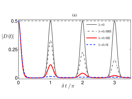
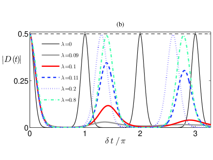
Figure 3: Norm of the decoherence factor without Markov approximation. (a) If the cavity-bath coupling strength is weak, the recovering amplitude of the decoherence factor decreases along with $\lambda$. (a) When the cavity-bath coupling strength is large enough, the recovering amplitude of the decoherence factor increases along with $\lambda$ but its recovering period is changed by the bath.

Next we numerically calculate the norm of decoherence factor with or without Markov approximation with parameters: $\omega_{0}=1$, $\delta=0.1$, $\left|\alpha\right|^{2}=5$, and $\Omega_{c}=10$. It is found that when the cavity-bath coupling is small ($\lambda=0.002$), the decoherence factors with or without Markov are nearly the same Figs. 2(a), but they diverge from each other when the coupling strength becomes large ($\lambda=0.01$) as in Figs. 2(b). And the Markov approximation loses its validity in strong-coupling regime ($\lambda=0.1$). From the insets of Figs. 2(a-c), we find that the Markov approximation also becomes invalid for a short-time dynamics (the norm of the decoherence factor under Markov approximation exceeds $0.5$).

When the cavity-bath coupling is weak, the decoherence factor without Markov approximation will still revive at $\delta t=n\pi,(n=1,2,3,\dots)$, but the recovering amplitude decreases along with the cavity-bath coupling $\lambda$ and will decay to $0$ finally (Fig. 3 (a)), due to the dephasing of the cavity field induced by the bath. On the contrary, if the cavity-bath coupling becomes strong enough, the reviving magnitude will increase with the coupling strength $\lambda$ (Fig. 3(b)). Especially, when the coupling strength become to be ultra-strong ($\lambda>0.1$), the recovering amplitude almost does not decay, just like that the bath does not exist. This is because when $\lambda>\omega_{0}/\Omega_{c}=0.1$ (for Ohmic bath), the cavity will stay in the system-bath coupling-induced dissipationless localized mode arXiv12_WMZhang . As a result, the recovering amplitude almost does not decay but the recovering period is shifted.

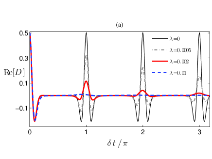
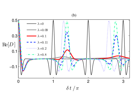
Figure 4: Ramsey interference is used to detect the decoherence factor. (a) Real part of the decoherence factor in weak coupling region without the Markov approximation. (b) Real part of the decoherence factor in strong coupling region without the Markov approximation.

Finally, we can utilize the Ramsey interference to detect the decoherence factor. After interacting with the cavity, the atom undergoes an additional resonant microwave $\pi/2$ pulse performing the following transformation

$$\left|e\right\rangle\rightarrow\frac{1}{\sqrt{2}}\left(\left|e\right\rangle+\left|g\right\rangle\right),\ \left|g\right\rangle\rightarrow\frac{1}{\sqrt{2}}\left(-\left|e\right\rangle+\left|g\right\rangle\right).$$

And it is found that (please refer to Appendix E for the detailed calculation)

$$\mathrm{Re}[D\left(t\right)]=\frac{1}{2}\left[\Pi_{g}\left(t\right)-\Pi_{e}\left(t\right)\right],$$ (51)

where

$$\Pi_{\sigma}=e^{-\left|\alpha\right|^{2}}\mathrm{Tr}_{f}\left\{\left\langle\sigma\right|e^{-i\theta\sigma_{y}/2}\rho_{a-f}e^{i\theta\sigma_{y}/2}\left|\sigma\right\rangle\right\},$$ (52)

is the population of the atoms in the rotated state $\exp(i\theta\sigma_{y}/2)\left|\sigma\right\rangle(\sigma=g,e)$ with rotation angle $\theta=\pi/2$ corresponding to the final $\pi/2$ pulse. Thus we can measure the real part of the decoherence factor through detecting the population difference of the out-coming atom. As shown in Figs. 4, the real part of the decoherence factor can also reflect the non-Markovianity of the bath.

VI SUMMERY

By constructing the reduced density matrix from the formal solution of the Heisenberg equations, we revisited the exact non-Markovian master equations for open quantum systems of Bose or Fermi type. The non-Markovianity can be reflected by the time-dependent decay coefficients such as $\Gamma\left(t\right)$ and $\tilde{\Gamma}\left(t\right)$, with historical memory. To probe the non-Markovianity of the dissipation of the single model EM field in a cavity, we let large detuning atoms pass through the cavity. It displayed that the non-Markovianity of the bath is explicitly reflected by the atomic decoherence factor. In the week coupling regime, the periodically reviving amplitude decreases along with the cavity-bath coupling strength $\lambda$ and decays to $0$ finally. However, in the strong coupling regime, the reviving amplitude increases with $\lambda$ and almost does not decay in the ultra-strong coupling case. But the recovering period is shifted by the bath. We expect our results to be verified by experiments.

Appendix A BOSON AND FERMION COHERENT STATES

A.1 Boson coherent state

For an arbitrary complex number $\alpha=r\exp\left(i\varphi\right)$, the coherent state of a Bose mode with frequency $\omega_{0}$ could be defined as

$$\left|\alpha\right\rangle\equiv e^{\alpha a^{\dagger}}\left|0\right\rangle=\sum_{n=0}^{\infty}\frac{\alpha^{n}}{\sqrt{n!}}\left|n\right\rangle,$$ (53)

where $a^{\dagger}$ is the creation operator of the boson and $\left|n\right\rangle$ is the $n$th Fock state. It is found that the coherent state defined in Eq. (53) is not normalized and different coherent states are generally not orthogonal

$$\left\langle\alpha\mid\alpha^{\prime}\right\rangle=\left\langle 0\right|e^{\alpha^{*}a}e^{\alpha^{\prime}a^{\dagger}}\left|0\right\rangle=\exp\left(\alpha^{*}\alpha^{\prime}\right).$$ (54)

All the coherent states form an over-complete sets

$$\int d\mu\left(\alpha\right)\left|\alpha\right\rangle\left\langle\alpha\right|=1,$$ (55)

with the measures

$$d\mu\left(\alpha\right)\equiv e^{-\left|\alpha\right|^{2}}\frac{d^{2}\alpha}{\pi}=e^{-\left|\alpha\right|^{2}}\frac{r}{\pi}drd\varphi.$$ (56)

And the density matrix of the thermal equilibrium state in this coherent-state representation reads

$$\rho_{T} = \frac{1}{1+f(\omega_{0})}\exp\left(-\beta\omega_{0}a^{\dagger}a\right)$$ (57)

$$= \int d\mu\left(\alpha\right)\frac{1}{f(\omega_{0})}\exp\left[-\frac{\left|\alpha\right|^{2}}{f(\omega_{0})}\right]\left|\alpha\right\rangle\left\langle a\right|,$$ (58)

where $f\left(\omega_{0}\right)=1/\left[\exp(\beta\omega_{0})-1\right]$ is the mean occupation number, with temperature $T=1/(k_{B}\beta)$.

A.2 Fermion coherent state

The fermion coherent state is defined of a similar form as bosons

$$\left|\alpha\right\rangle\equiv e^{-\alpha a^{\dagger}}\left|0\right\rangle.$$ (59)

The only difference lies in the fact that $\alpha$ is a generator of a Grassmann algebra instead of an ordinary complex number and $a^{\dagger}$ is the creation operator for Fermi particles and they satisfy the anti-commutation relations

$$\left\{\alpha,\alpha^{\prime}\right\}=\left\{\alpha,a\right\}=\left\{\alpha,a^{\dagger}\right\}=0.$$ (60)

The overlap of two fermion coherent states is

$$\left\langle\alpha\mid\alpha^{\prime}\right\rangle=\exp\left(\alpha^{*}\alpha^{\prime}\right),$$ (61)

and the completeness relation reads

$$\int d\mu\left(\alpha\right)\left|\alpha\right\rangle\left\langle\alpha\right|=1,$$ (62)

with

$$d\mu\left(\alpha\right)=d\alpha^{*}d\alpha e^{-\alpha^{*}\alpha}.$$ (63)

Appendix B Constrains of blocks of $\mathcal{U}\left(t\right)$

Due to hermiticity of matrix $\mathcal{H}$, the time-evolution operator $\mathcal{U}\left(t\right)$ in Liouville space is a unitary matrix, i.e.,

$$\left[\begin{array}[]{cc}W\left(t\right)&T\left(t\right)\\ P\left(t\right)&Q\left(t\right)\end{array}\right]\left[\begin{array}[]{cc}W^{\dagger}\left(t\right)&P^{\dagger}\left(t\right)\\ T^{\dagger}\left(t\right)&Q^{\dagger}\left(t\right)\end{array}\right]=I,$$ (64)

which leads to

$$WW^{\dagger}+TT^{\dagger}=I,$$ (65)

$$PP^{\dagger}+QQ^{\dagger}=I,$$ (66)

$$WP^{\dagger}+TQ^{\dagger}=\mathbf{0},$$ (67)

$$PW^{\dagger}+QT^{\dagger} = \mathbf{0}.$$ (68)

Except some special time $t$, the matrices $W\left(t\right)$ and $Q\left(t\right)$ are reversible. Then we have

$$P=-QT^{\dagger}\left(W^{\dagger}\right)^{-1},$$ (69)

$$P^{\dagger} = -W^{-1}TQ^{\dagger}.$$ (70)

Appendix C CALCULATION OF THE PROPAGATING FUNCTION

The reduced density matrix $\rho_{s}\left(t\right)$ of the system is obtained by tracing over the degrees of freedom of $B$ in $\rho\left(t\right)$

$$\rho_{s}\left(t\right) \!\!= \int d\mu\!\left(\vec{z}\right)\!\left\langle\vec{z}\right|\!\rho\left(t\right)\!\left|\vec{z}\right\rangle$$ (71)

$$\equiv \int\!\!d\mu\!\left(\vec{\alpha},\vec{\alpha}^{\prime}\right)\!\rho_{s}\left(\vec{\alpha},\vec{\alpha}^{\prime};t\right)\!\left|\vec{\alpha}\right\rangle\!\left\langle\vec{\alpha}^{\prime}\right|,$$ (72)

where $\left|\vec{\alpha}\right\rangle(\left|\vec{\alpha}^{\prime}\right\rangle)$ and $\left|\vec{z}\right\rangle$ are coherent states of $S$ and $B$, respectively. The element of the reduced density matrix is explicitly given by

$$\!\!\!\!\!\!\!\!\!\!\rho_{s}\left(\vec{\alpha},\vec{\alpha}^{\prime};t\right) = \int d\mu\!\left(\vec{z}\right)\!\left\langle\vec{\alpha},\vec{z}\right|\!\rho\left(t\right)\!\left|\vec{\alpha}^{\prime},\vec{z}\right\rangle$$ (74)

$$\!\!\!\!\!\!\!\!\!\!\!= \!\!\!\int\!\!d\mu\!\left(\vec{z}\right)\!d\mu\!\left(\!\vec{\xi},\!\vec{z}^{\prime}\!,\vec{\xi}^{\prime}\!,\!\vec{z}^{\prime\prime}\!\right)\left\langle\vec{\alpha},\vec{z}\right|\!U\!\left(t\right)\!\left|\vec{\xi},\vec{z}^{\prime}\right\rangle$$

$$\!\!\!\!\!\!\!\!\!\!\!\!\!\times\!\left\langle\!\vec{\xi},\vec{z}^{\prime}\right|\!\rho_{s}\!\left(0\right)\!\rho_{b}\!\left(0\right)\!\left|\!\vec{\xi}^{\prime},\vec{z}^{\prime\prime}\!\right\rangle\!\!\left\langle\!\vec{\xi}^{\prime},\vec{z}^{\prime\prime}\right|\!U^{\dagger}\!\left|\vec{\alpha}^{\prime},\vec{z}\right\rangle$$

$$\!\!\!\!\!\!\!\!\!\!\!\!\!\!\!\equiv \!\!\!\!\!\!\!\!\!\int\!\!\!d\mu\!\left(\!\vec{\xi},\vec{\xi}^{\prime}\!\right)\!K\!\left(\vec{\alpha}^{\dagger},\vec{\alpha}^{\prime},\vec{\xi},\vec{\xi}^{\prime\dagger},t\right)\!\!\left\langle\vec{\xi}\right|\!\rho_{s}\!\left(0\right)\!\left|\vec{\xi}^{\prime}\right\rangle\!\!,$$ (75)

with

$$K = \int d\mu\!\left(\vec{z}\right)\left\langle\vec{\alpha},\vec{z}\right|U\left(t\right)\left|\vec{\xi}\right\rangle$$ (76)

$$\times\!\left\langle\vec{\xi}^{\prime}\right|\rho_{b}\left(0\right)U^{\dagger}\left(t\right)\left|\vec{\alpha}^{\prime},\vec{z}\right\rangle.$$

Here, we have used the fact the initial state of the total system is of the direct product form and the completeness of the coherent states $\left\{\left|\vec{z}^{\prime}\right\rangle\right\}$ and $\left\{\left|\vec{z}^{\prime\prime}\right\rangle\right\}$ of the bath.

With the help of Eqs. (9), (10), (25), (24), and (26), the propagator is re-expressed in terms of the coefficient matrices

$$K\left(\vec{\alpha}^{\dagger},\vec{\alpha}^{\prime},\vec{\xi},\vec{\xi}^{\prime\dagger};t\right)$$ (77)

$$= \int d\mu\left(\vec{z}\right)\left\langle W^{\dagger}\vec{\alpha}+P^{\dagger}\vec{z}\mid\vec{\xi}\right\rangle\left\langle\vec{\xi}^{\prime}\mid W^{\dagger}\vec{\alpha}^{\prime}+P^{\dagger}\vec{z}\right\rangle$$

$$\!\!\!\!\!\!\!\!\!\times\!\left(\!\!\prod_{l}\!\frac{1}{f_{l}\!+\!1}\!\!\right)\!\left\langle T^{\dagger}\!\vec{\alpha}\!+\!Q^{\dagger}\vec{z}\right|\!\exp\!\!\left[\!-\!\vec{b}^{\dagger}\!\beta E\vec{b}\right]\!\!\left|T^{\dagger}\!\vec{\alpha}^{\prime}\!+\!Q^{\dagger}\!\vec{z}\right\rangle\!\!.$$

Using formulas $\left\langle\alpha\right|\exp\left(\delta b^{\dagger}b\right)\left|\alpha^{\prime}\right\rangle=\exp\left[\alpha^{*}\alpha^{\prime}\exp\left(\delta\right)\right]$ and

$$\int d\mu\left(\vec{z}\right)e^{\vec{z}^{\dagger}D\vec{z}+\vec{u}^{\dagger}\cdot\vec{z}+\vec{z}^{\dagger}\cdot\vec{v}}=\frac{\exp\left[\vec{u}^{\dagger}\left(I-D\right)^{-1}\vec{v}\right]}{\mathrm{det}\left[I-D\right]},$$ (78)

(for any $N_{s}\times N_{s}$ Hermitian matrix $D$ makes $\left(I-D\right)$ positive-definite), one goes to

$$\!\!\!\!\!\!\!\!\!\!\!\!\!K(\vec{\alpha}^{\dagger},\vec{\alpha}^{\prime},\vec{\xi},\vec{\xi}^{\prime\dagger},t)\! = \!A(t)\!\exp\!\!\left[\!\!\begin{array}[]{c}\vec{\alpha}^{\dagger}J_{1}(t)\vec{\xi}+\vec{\xi}^{\prime\dagger}J_{1}^{\dagger}(t)\vec{\alpha}^{\prime}\\ +\vec{\alpha}^{\dagger}J_{2}(t)\vec{\alpha}^{\prime}+\vec{\xi}^{\prime\dagger}J_{3}\vec{\xi}\!\!\!\!\end{array}\right]\!,$$ (81)

where

$$A=\left(\prod_{l}\frac{1}{f_{l}\!+\!1}\right)\mathrm{det}\left[I-Qf\left(I+f\right)^{-1}Q^{\dagger}\right]^{-1},$$ (82)

$$\!\!J_{1}\!=W\!+\!Tf\!\left(I\!+\!f\right)^{-1}\!Q^{\dagger}\!\!\left[I\!-\!Qf\!\left(I\!+\!f\right)^{-1}\!Q^{\dagger}\right]^{-1}\!\!\!P\!\!,$$ (83)

$$\!\!\!\!\!\!\!\!\!\!\!\!J_{2} = Tf\!\left(I\!+\!f\right)^{-1}T^{\dagger}+\!T\!f\!\left(I\!+\!f\right)^{-1}\!Q^{\dagger}$$ (84)

$$\times\left[I-Qf\left(I\!+\!f\right)^{-1}\!Q^{\dagger}\right]^{-1}\!Q\!f\!\left(I\!+\!f\right)^{-1}T^{\dagger},$$

$$J_{3} = P^{\dagger}\left[I-Qf\left(I\!+\!f\right)^{-1}\!Q^{\dagger}\right]^{-1}\!P,$$ (85)

and we have introduced a diagonal matrix $f=\mathrm{diag}[f_{1},f_{2},\cdots,f_{N_{b}}]$.

Then we will deal with these four terms one by one. First we make some pretreatment to obtain an expanding series. From Eqs. (66), (69), and (70), one finds

$$\!I\!-\!Q\!f\!\left(I\!+\!f\right)^{-1}\!\!Q^{\dagger}\!\!=\!\!Q\!\!\left[T^{\dagger}\!\left(WW^{\dagger}\right)^{-1}\!\!T\!+\!\left(\!I\!+\!f\right)^{-1}\right]\!Q^{\dagger}\!\!.\!\!\!\!\!$$ (86)

So that

$$\left[I-Qf\left(I\!+\!f\right)^{-1}\!Q^{\dagger}\right]^{-1}$$ (87)

$$=\!\! \left(Q^{\dagger}\right)^{-1}\!\!\left(\!I\!+\!f\right)\!\!\sum_{n=0}^{\infty}\!\left(-1\right)^{n}\!\!\left[\!T^{\dagger}\!\!\left(WW^{\dagger}\right)^{-1}\!T\!\left(I\!+\!f\right)\right]^{n}\!\!Q^{-1}\!\!\!.$$

C.1 $J_{1}\left(t\right)$, $J_{2}\left(t\right)$, and $J_{3}\left(t\right)$

According to Eqs. (69), (83), and (87), $J_{1}\left(t\right)$ is explicitly expanded to

$$J_{1} = W-Tf\sum_{n=0}^{\infty}\left(-1\right)^{n}\!\!\left[\!T^{\dagger}\!\!\left(WW^{\dagger}\right)^{-1}\!T\!\left(I\!+\!f\right)\right]^{n}T^{\dagger}\left(W^{\dagger}\right)^{-1}$$ (88)

$$= W-TfT^{\dagger}\sum_{n=0}^{\infty}\left(-1\right)^{n}\!\!\left[\!\!\left(WW^{\dagger}\right)^{-1}\!T\!\left(I\!+\!f\right)T^{\dagger}\!\right]^{n}\left(W^{\dagger}\right)^{-1}$$

$$= W-V\left[1+\left(WW^{\dagger}\right)^{-1}\!T\!\left(I\!+\!f\right)T^{\dagger}\right]^{-1}\left(W^{\dagger}\right)^{-1}$$

$$= W-V\left[WW^{\dagger}+T\!\left(I\!+\!f\right)T^{\dagger}\right]^{-1}W$$

$$= \left(1+V\right)^{-1}W.$$ (89)

The third step we have introduced a new $N_{s}\times N_{s}$-matrix $V\left(t\right)=T\left(t\right)fT^{\dagger}\left(t\right)$. Similarly, one obtains

$$J_{3}=I-W^{\dagger}\left(1+V\right)^{-1}W.$$ (90)

The calculation of $J_{2}$ is a little more complicated

$$\!\!\!\!\!\!\!\!\!J_{2} = T\left\{I+\!f\!\sum_{n=0}^{\infty}\left(-1\right)^{n}\!\!\left[\!T^{\dagger}\!\!\left(WW^{\dagger}\right)^{-1}\!T\!\left(I\!+\!f\right)\right]^{n}\right\}$$ (94)

$$\times f\!\left(I\!+\!f\right)^{-1}T^{\dagger}$$

$$= V+Tf\left(\sum_{n=1}^{\infty}\left(-1\right)^{n}\!\!\left[\!T^{\dagger}\!\!\left(WW^{\dagger}\right)^{-1}\!T\!\left(I\!+\!f\right)\right]^{n-1}\right)$$

$$\times T^{\dagger}\left(WW^{\dagger}\right)^{-1}TfT^{\dagger}$$

$$= V+Tf\left(\sum_{n=1}^{\infty}\left(-1\right)^{n}\!\!\left[\!T^{\dagger}\!\!\left(WW^{\dagger}\right)^{-1}\!T\!\left(I\!+\!f\right)\right]^{n-1}\right)$$

$$\times T^{\dagger}\left(WW^{\dagger}\right)^{-1}T\left(I+f-I\right)T^{\dagger}$$

$$= V\left\{I+\sum_{n=1}^{\infty}\left(-1\right)^{n}\!\!\left[\!\left(WW^{\dagger}\right)^{-1}\!T\!\left(I\!+\!f\right)\!T^{\dagger}\!\right]^{n}\right\}$$

$$\!\!\!\!\!\!+V\!\!\sum_{n=0}^{\infty}\!\left(\!-1\right)^{n}\!\!\left[\!\left(W\!W^{\dagger}\!\right)^{-1}\!T\!\left(I\!+\!f\right)\!T^{\dagger}\!\right]^{n}\!\!\!\left(\!W\!W^{\dagger}\right)^{\!-1}\!\!\!TT^{\dagger}$$

$$= V\left[WW^{\dagger}+T\left(I+f\right)T^{\dagger}\right]^{-1}\left(WW^{\dagger}+TT^{\dagger}\right)$$ (95)

$$= V\left(I+V\right)^{-1}.$$ (96)

C.2 $A\left(t\right)$

The matrix $A\left(t\right)$ is determined by the normalization condition,

$$\!\!\!1 = \mathrm{Tr}\!\left[\rho_{s}\!\left(\!t\!\right)\right]$$ (97)

$$= \int\!\!\!d\!\!\mu\!\left(\vec{\alpha}\right)\!\!d\!\mu\!\!\left(\vec{\xi},\vec{\xi}^{\prime}\right)\!\!K\!\!\left(\!\vec{\alpha},\!\vec{\alpha},\!\vec{\xi},\!\vec{\xi}^{\prime}\!,t\right)\!\!\left\langle\!\vec{\xi}\right|\!\rho_{s}\!\left(0\right)\!\left|\!\vec{\xi}^{\prime}\right\rangle$$ (98)

$$= A\mathrm{det}\!\left[I\!+\!V\right]\!\!\!\int\!\!d\!\mu\!\!\left(\!\vec{\xi},\vec{\xi}^{\prime}\right)\!\!\left\langle\!\vec{\xi}\right|\!\rho_{s}\!\left(0\right)\!\left|\!\vec{\xi}^{\prime}\right\rangle\!\exp\!\left(\!\vec{\xi}^{\prime\dagger}\!\cdot\!\vec{\xi}\right)$$ (99)

$$= A\mathrm{det}\left[I+V\right]\int\!\!d\!\mu\!\!\left(\vec{\xi}\right)\!\!\left\langle\!\vec{\xi}\right|\!\rho_{s}\!\left(0\right)\!\left|\!\vec{\xi}\right\rangle.$$ (100)

In the second step, we carried out the integral over $\vec{\alpha}$ of Eq. (29) and used the identity

$$J_{3}\left(t\right)+J_{1}^{\dagger}\left(I+V\right)J_{1}\left(t\right)=I.$$ (101)

And the last step, the following formula is used

$$\int d\mu\left(\alpha^{\prime}\right)\left(\alpha^{\prime}\right)^{n}e^{\alpha^{\prime*}\alpha}=\alpha^{n}.$$ (102)

Since the initial density matrix is also normalized, thus

$$A\left(t\right)=\mathrm{det}\left[\left(I+V\right)^{-1}\right].$$

Appendix D TIME DIFFERENTIAL OF THE PROPAGATING FUNCTION

The time differential of the propagating function is given by

$$\dot{K}=\left[\frac{\dot{A}}{A}\!+\!\vec{\alpha}^{\dagger}\dot{J}_{1}\vec{\xi}\!+\!\vec{\xi}^{\prime\dagger}\dot{J}_{1}^{\dagger}\vec{\alpha}^{\prime}\!+\!\vec{\alpha}^{\dagger}\dot{J}_{2}\vec{\alpha}^{\prime}\!+\!\vec{\xi}^{\prime\dagger}\dot{J}_{3}\vec{\xi}\right]K.$$ (103)

We define the differential operators

$$\overset{\rightarrow}{\nabla}_{\alpha^{*}}\equiv\left[\frac{\partial}{\partial\alpha_{1}^{*}},\frac{\partial}{\partial\alpha_{2}^{*}},\cdots,\frac{\partial}{\partial\alpha_{N_{s}}^{*}}\right]^{T},$$ (104)

and

$$\overset{\rightarrow}{\nabla}_{\alpha}^{T} \equiv \left[\frac{\partial}{\partial\alpha_{1}},\frac{\partial}{\partial\alpha_{2}},\cdots,\frac{\partial}{\partial\alpha_{N_{s}}}\right].$$ (105)

It is ready to find that

$$\vec{\xi}K=J_{1}^{-1}\left(\overset{\rightarrow}{\nabla}_{\alpha^{*}}-J_{2}\vec{\alpha}^{\prime}\right)K,$$ (106)

$$\vec{\xi}^{\prime\dagger}K=\left(\overset{\rightarrow}{\nabla}_{\alpha^{\prime}}^{T}-\vec{\alpha}^{\dagger}J_{2}\right)\left(J_{1}^{\dagger}\right)^{-1}K,$$ (107)

$$\!\!\!\!\!\!\!\!\vec{\xi}^{\prime\dagger}\!K\!\vec{\xi} \!\!=\!\!\! \left(\!\overset{\rightarrow}{\nabla}_{\alpha^{\prime}}^{T}\!-\!\vec{\alpha}^{\dagger}\!J_{2}\!\!\right)\!\left(\!J_{1}^{\dagger}\!\right)^{-1}\!\!J_{1}^{-1}\!\!\left(\!\overset{\rightarrow}{\nabla}_{\alpha^{*}}\!-\!J_{2}\vec{\alpha}^{\prime}\!\right)\!K.$$ (108)

These relations lead to

$$\dot{K}\!\! =\!\! \vec{\alpha}^{\dagger}\!\!\left[\!\dot{J}_{2}\!-\!\dot{J}_{1}\!J_{1}^{-1}J_{2}\!\!-\!J_{2}\!\left(\!J_{1}^{\dagger}\!\right)^{-1}\!\!\dot{J}_{1}^{\dagger}\!+\!J_{2}\!\left(\!J_{1}^{\dagger}\!\right)^{-1}\!\!\dot{J}_{3}J_{1}^{-1}\!J_{2}\!\right]\!\!K\!\vec{\alpha}^{\prime}$$ (110)

$$+\left\{\frac{\dot{A}}{A}-\mathrm{Tr}\left[\left(J_{1}^{\dagger}\right)^{-1}\dot{J}_{3}J_{1}^{-1}J_{2}\right]\right\}K$$

$$+\vec{\alpha}^{\dagger}\left[\!\dot{J}_{1}\!J_{1}^{-1}-\!J_{2}\!\left(\!J_{1}^{\dagger}\!\right)^{-1}\!\!\dot{J}_{3}J_{1}^{-1}\!\right]\overset{\rightarrow}{\nabla}_{\alpha^{*}}K$$

$$+\left(\overset{\rightarrow}{\nabla}_{\alpha^{\prime}}^{T}\!K\right)\left[\!\left(\!J_{1}^{\dagger}\!\right)^{-1}\!\!\dot{J}_{1}^{\dagger}-\left(\!J_{1}^{\dagger}\!\right)^{-1}\!\!\dot{J}_{3}J_{1}^{-1}\!J_{2}\!\right]\vec{\alpha}^{\prime}$$

$$+\overset{\rightarrow}{\nabla}_{\alpha^{\prime}}^{T}\!\left(\!J_{1}^{\dagger}\!\right)^{-1}\!\!\dot{J}_{3}J_{1}^{-1}\overset{\rightarrow}{\nabla}_{\alpha^{*}}K$$

$$\equiv \vec{\alpha}^{\dagger}\tilde{\Gamma}K\vec{\alpha}^{\prime}-\mathrm{Tr}\left[\tilde{\Gamma}\right]K-\vec{\alpha}^{\dagger}\left(\Gamma+\mathrm{i}\tilde{\Omega}+\tilde{\Gamma}\right)\overset{\rightarrow}{\nabla}_{\alpha^{*}}K$$

$$-\!\left(\!\overset{\rightarrow}{\nabla}_{\alpha^{\prime}}^{T}\!K\!\right)\!\!\left(\Gamma\!-\mathrm{i}\tilde{\Omega}\!+\!\tilde{\Gamma}\!\right)\!\vec{\alpha}^{\prime}\!+\!\overset{\rightarrow}{\nabla}_{\alpha^{\prime}}^{T}\!\left(\tilde{\Gamma}\!+\!2\Gamma\!\right)\!\overset{\rightarrow}{\nabla}_{\alpha^{*}}\!K\!,$$

with Hermitian matrices

$$\tilde{\Gamma}=\dot{V}-\dot{W}W^{-1}V-V\left(\dot{W}W^{-1}\right)^{\dagger},$$ (111)

$$\Gamma=-\frac{1}{2}\left[\dot{W}W^{-1}+\left(\dot{W}W^{-1}\right)^{\dagger}\right],$$ (112)

and

$$\tilde{\Omega}=\frac{\mathrm{i}}{2}\left[\dot{W}W^{-1}-\left(\dot{W}W^{-1}\right)^{\dagger}\right].$$ (113)

The last step the following relations have been used

$$\!\!\!\!\!\!\!\!\!\!\!\!\!\!\!\!\!\!\!\dot{J}_{1}\!J_{1}^{-1}\!\! = \!\!\left[\!\frac{d}{dt}\!\!\left(I\!+\!V\right)^{-1}\!\right]\!\!\!\left(I\!+\!V\right)\!\!+\!\!\left(I\!+\!V\right)^{-1}\!\!\left(\!\dot{W}W^{-1}\!\right)\!\!\left(I\!\!+\!\!V\right)$$ (115)

$$= -\left[\left(I+V\right)^{-1}\dot{V}\left(I+V\right)^{-1}\right]\left(I+V\right)$$

$$+\left(I+V\right)^{-1}\left(\dot{W}W^{-1}\right)\left(I+V\right)$$

$$= \!\!-\!\left(I\!+\!V\right)^{-1}\!\!\left[\dot{V}-\!\!\left(\!\dot{W}W^{-1}\!\right)\!\!\left(I\!+V\right)\!\right]\!\!,$$ (116)

$$\left(\!J_{1}^{\dagger}\!\right)^{-1}\!\!\!\dot{J}_{3}J_{1}^{-1}\!\!=\!\!-\!\left(I\!\!+\!\!V\!\right)\!\!\left(\!\dot{W}\!W^{-1}\!\right)^{\dagger}\!\!\!-\!\dot{W}\!W^{-1}\!\!\left(I\!\!+\!\!V\right)\!+\!\dot{V}\!,$$ (117)

and

$$\frac{\dot{A}}{A}-\mathrm{Tr}\left[\left(J_{1}^{\dagger}\right)^{-1}\dot{J}_{3}J_{1}^{-1}J_{2}\right]$$ (120)

$$=\!\! \frac{d}{dt}\mathrm{ln}A\!+\!\mathrm{Tr}\!\left[\begin{array}[]{c}\!\!V\left(\dot{W}W^{-1}\!\right)^{\dagger}\!+\!\left(\!\dot{W}W^{-1}\!\right)\!\!V\!\!\\ -\dot{V}\left[I-\left(I+V\right)^{-1}\right]\end{array}\right]$$

$$= \!\!\frac{d}{dt}\mathrm{Tr}\!\left[\mathrm{ln}\left(I\!+\!V\right)^{-1}\right]\!+\!\mathrm{Tr}\!\left[-\tilde{\Gamma}\!+\!\dot{V}\!\left(I\!+\!V\right)^{-1}\!\right]$$ (121)

$$= -\mathrm{Tr}\left[\tilde{\Gamma}\right]$$ (122)

Appendix E DECOHERENCE FACTOR

Through the approach in Appendix C, we can obtain the element of the reduced density in Eq (47)

$$\rho_{a-f}\left(\!\alpha_{f},\sigma;\alpha_{f}^{\prime},\sigma^{\prime}\!\right)$$ (125)

$$= \frac{1}{2}A_{\sigma\sigma^{\prime}}\exp\left[\begin{array}[]{c}\alpha_{f}^{*}J_{1,\sigma\sigma^{\prime}}\alpha+\alpha^{*}J_{1,\sigma^{\prime}\sigma}^{\dagger}\alpha_{f}^{\prime}\\ +\alpha_{f}^{*}J_{2,\sigma\sigma^{\prime}}\alpha_{f}^{\prime}+\alpha^{*}J_{3,\sigma\sigma^{\prime}}\alpha\end{array}\right],$$

where in the case of zero temperature bath

$$\!A_{\sigma\sigma^{\prime}}\!=\!1,J_{1,\sigma\sigma^{\prime}}\!=\!W_{\sigma}\left(t\right),J_{2,\sigma\sigma^{\prime}}\!=\!0,J_{3,\sigma\sigma^{\prime}}\!=\!P_{\sigma^{\prime}}^{\dagger}P_{\sigma}.\!\!\!\!$$ (126)

Here $W_{\sigma}$ is determined by Eq. (18) with $M=\omega_{0}\pm\delta$ ($\pm$ corresponding to $\left|e\right\rangle$ and $\left|g\right\rangle$ states, respectively) and $P_{\sigma}$ is given by Eq. (16). Following from Eq. (48), we find that the population difference of the out-coming atom just gives the decoherence factor

$$\Pi_{g}\left(t\right)-\Pi_{e}\left(t\right)$$ (129)

$$= e^{-\left|\alpha\right|^{2}}\mathrm{Tr}_{f}\left\{\begin{array}[]{c}\left\langle g\right|e^{-i\theta\sigma_{y}/2}\rho_{a-f}e^{i\theta\sigma_{y}/2}\left|g\right\rangle\\ -\left\langle e\right|e^{-i\theta\sigma_{y}/2}\rho_{a-f}e^{i\theta\sigma_{y}/2}\left|e\right\rangle\end{array}\right\}$$

$$= D\left(t\right),$$ (130)

where $\theta=\pi/2$ and $\sigma_{y}=i\left(\left|g\right\rangle\left\langle e\right|-\left|e\right\rangle\left\langle g\right|\right)$. With the help of Eq. (125), we obtain the decoherence factor as

$$D\left(t\right)\!\!=\!\!\mathrm{Re}\!\left\{\!\exp\!\left[\!\left(\!W_{\sigma}^{*}\!\left(t\right)\!W_{\sigma^{\prime}}\!\left(t\right)\!+\!J_{3,\sigma\sigma^{\prime}}\!\left(t\right)\!-\!1\!\right)\!\left|\alpha\right|^{2}\!\right]\!\right\}\!.\!\!$$ (131)

References

(1)E. Kanai, Prog. Theor. Phys. 3,
440 (1948).
(2)P. Caldirola, Nuovo Cimento 18,
393 (1941).
(3)L. H. Yu and C. P. Sun, Phys. Rev. A 49,
592 (1994).
(4)C. P. Sun and L. H. Yu, Phys. Rev. A 51,
1845 (1995).
(5)C. P. Sun, Y. B. Gao, H. F. Dong, and S. R. Zhao,
Phys. Rev. E 57, 3900 (1998).
(6)A. O. Caldeira and A. J. Leggett, Ann. Phys.
(N. Y.) 149, 374 (1983).
(7)H.-P. Breuer and F. Petruccione, The Theory
of Open Quantum Systems, (Oxford University Press, Oxford, 2002).
(8)M. Lax, J. Phys. Chem. Solids 25,
487 (1964); Phys. Rev. A, 145, 110 (1966).
(9)W. H. Louisell, Quantum Statistical Properties
of Radiation, (John Wiley and Sons, New York, 1973), Chapter 7.
(10)B. L. Hu, J. P. Paz, and Y. H. Zhang, Phys. Rev.
D 45, 2843 (1992); J. J. Halliwell and T. Yu, Phys. Rev.
D 53, 2012 (1996).
(11)T. Yu, Phys. Rev. A 69, 062107 (2004).
(12)J. H. An and W. M. Zhang, Phys. Rev. A 76,
042127 (2007); J. H. An, M. Feng, and W. M. Zhang, Quantum Inf. Comput.
9, 0317 (2009).
(13)C. U. Lei and W. M. Zhang, Ann. Phys. 327,
1048 (2012).
(14)M. W. Y. Tu and W. M. Zhang, Phys. Rev. B 78,
235311 (2008).
(15)J. S. Jin, M. W. Y. Tu, W. M. Zhang, and Y.
J. Yan, New J. Phys. 12, 086013 (2010).
(16)H. N. Xiong, W. M. Zhang, X. G. Wang, and M. H.
Wu, Phys. Rev. A 82, 012105 (2010).
(17)B. Vacchini and H.-P. Breuer, Phys. Rev. A
81, 042103 (2010).
(18)H. F. Li and Jiushu Shao, e-print arXiv:1205.4616.
(19)H.-P. Breuer, E.-M. Laine, and J. Piilo, Phys.
Rev. Lett. 103, 210401 (2009).
(20)X. M. Lu, X. G Wang, and C. P. Sun, Phys. Rev.
A 82, 042103 (2010).
(21)W. M. Zhang, P. Y. Lo, H. N. Xiong, M. W. Y. Tu, and F. Nori,
Phys. Rev. Lett. 109, 170402 (2012).
(22)A. Vourdas and R. F. Bishop, Phy.
Rev. A 50, 3331 (1994).
(23)L. D. Faddeev and A. A. Slavnov, Gauge
Fields: Introduction to Quantum Theory, (Benjamin-Cummings, Reading,
MA, 1980).
(24)A. Das, Quantum Theory: A Path Integral Approach,
(World Scientific, 2006).
(25)V. B. Braginshy, F. Y. Khalili, K. S.
Thorne, Quantum Measurement (Cambridge University Press,
Cambridge, UK, 1995).
(26)M. Brune, S. Haroche, V. Lefevre, J. M. Raimond,
and N. Zagury, Phys. Rev. Lett. 65, 976 (1990).
(27)M. Brune, S. Haroche, J. M. Raimond, L. Davidovich,
and N. Zagury, Phys. Rev. A 45, 5193 (1992).
(28)H. T. Quan, Z. Song, X. F. Liu, P. Zanardi,
and C. P. Sun, Phys. Rev. Lett. 96, 140604 (2006).
(29)Z. P. Karkuszewski, C. Jarzynski, and W. H. Zurek,
Phys. Rev. Lett. 89, 170405 (2002); F. M. Cucchietti, D.
A. R. Dalvit, J. P. Paz, and W. H. Zurek, ibid. 91,
210403 (2003); R. A.Jalabert and H. M. Pastawski, ibid. 86,
2490 (2001)
(30)M. O. Scully and M. S. Zubairy, Quantum Optics,
(Cambridge University Press, Cambridge, 1997).
(31)M. Brune, E. Hagley, J. Dreyer, X. Maitre,
A. Maali, C. Wunderlich, J. M. Raimond, and S. Haroche, Phys. Rev.
Lett. 77, 4887 (1996).
(32)J. M. Raimond, M. Brune, and S. Haroche,
Phys. Rev. Lett. 79, 1964 (1997).
(33)C. Kiefer, Phys. Rev. D 46, 1658 (1992);
C. P. Sun, X. F. Liu, D. L. Zhou, and S. X. Yu, Phys. Rev. A 63, 012111 (2000);
F. M. Cucchietti, J. P. Paz, and W. H. Zurek, Phys. Rev. A 72, 052113 (2005);
Z. Sun, X. G. Wang, and C. P. Sun, Phys. Rev. A 75, 062312 (2007).