Published in Phys. Rev. B. 84, 214509 (2011) [doi: 10.1103/PhysRevB.00.004500].
Surface States, Edge Currents and the Angular Momentum of Chiral p-wave Superfluids

Abstract

The spectra of fermionic excitations, pairing correlations and edge currents confined near the boundary of a chiral p-wave superfluid are calculated to leading order in $\hbar/p_{f}\xi$. Results for the energy- and momentum-resolved spectral functions, including the spectral current density, of a chiral p-wave superfluid near a confining boundary are reported. The spectral functions reveal the subtle role of the chiral edge states in relation to the edge current and the angular momentum of a chiral p-wave superfluid, including the rapid suppression of $L_{z}(T)$ for $0\lesssim T\ll T_{c}$ in the fully gapped 2D chiral superfluid. The edge current and ground-state angular momentum are shown to be sensitive to boundary conditions, and as a consequence the topology and geometry of the confining boundaries. For perfect specular boundaries the edge current accounts for the ground-state angular momentum, $L_{z}=(N/2)\hbar$, of a cylindrical disk of chiral superfluid with $N/2$ fermion pairs. Non-specular scattering can dramatically suppress the edge current. In the limit of perfect retro-reflection the edge states form a flat band of zero modes that are non-chiral and generate no edge current. For a chiral superfluid film confined in a cylindrical toroidal geometry the ground-state angular momentum is, in general, non-extensive, and can have a value ranging from $L_{z}>(N/2)\hbar$ to $L_{z}<-(N/2)\hbar$ depending on the ratio of the inner and outer radii and the degree of back scattering on the inner and outer surfaces. Non-extensive scaling of $L_{z}$, and the reversal of the ground-state angular momentum for a toroidal geometry, would provide a signature of broken time-reversal symmetry of the ground state of superfluid ³He-A, as well as direct observation of chiral edge currents.

.1 Introduction

Among the remarkable phases of liquid ³He is the A-phase. In addition to being a superfluid which supports persistent currents, this fluid is believed to possess a spontaneous mass current in its ground state. Ground state currents are associated with the chirality of Cooper pairs that condense to form the A-phase and conspire to produce a macroscopic angular momentum. Chirality is encoded in the p-wave orbital order parameter, $\Delta({\bf p})=\Delta\,{\bf p}\cdot\left(\hat{\bf m}+i\hat{\bf n}\right)/p_{f}=\Delta\sin\theta_{{\bf p}}\,e^{i\phi_{{\bf p}}}$, where ${\bf p}$ is the relative momentum of a Cooper pair, $\{\hat{\bf m},\hat{\bf n},\hat{\bf l}\}$ is an orthonormal triad of unit vectors that define the orbital coordinates of the Cooper pair wave function, and $\Delta\sim k_{B}T_{c}$ is the pairing energy.Vollhardt and Wölfle (1990) This order parameter is an eigenfunction of the orbital angular momentum along $\hat{\bf l}=\hat{\bf m}\times\hat{\bf n}$ with eigenvalue $+\hbar$. Such broken symmetries in bulk condensed matter systems have implications for the spectrum of excitations bound to surfaces and topological defects.Volovik (1992a) This phase breaks time-reversal symmetry as well as parity, and is realized at all pressures below melting in thin superfluid ³He-A films. In the 2D limit the Fermi surface is fully gapped, and belongs to the topological class of integer quantum Hall systems.Read and Green (2000); Volovik (1988, 1992b) The 2D A-phase is also representative of layered p-wave superconductors with broken time-reversal symmetry, e.g. the proposed order parameter for superconducting Sr₂RuO₄.Mackenzie and Maeno (2003)

The macroscopic manifestation of chiral order in ³He-A is the ground-state angular momentum, ${\bf L}=\int_{V}dV{\bf r}\times{\bf g}({\bf r})$, where ${\bf g}$ is the mass current density. For 2D chiral p-wave superfluids in the BCS limit, where the size of Cooper pairs is large compared to Fermi wavelength, $\xi\gg\hbar/p_{f}$, the ground state currents are predominantly confined to boundaries. I discuss effects of surface scattering on the pairing correlations, the fermionic spectrum and ground state currents in the vicinity of boundaries confining a chiral p-wave superfluid. Results for the spectral current density highlight the fermionic spectrum that is responsible for the edge current and the ground state angular momentum. The theory is extended to finite temperatures, non-specular boundaries and multiply connected geometries. The results reported here are discussed in context with the results of Kita,Kita (1998) and Stone and Roy.Stone and Roy (2004)

Starting from Bogoliubov’s equations in Sec. .2, I introduce Eileberger’s quasiclassical equation for the Nambu propagator that is the basis for investigating the pairing correlations, spectrum of surface states and edge currents for chiral p-wave superfluids. The bound-state spectrum and results for the spectral current density are discussed in Secs. .3 and .4. Analysis of the continuum spectrum, edge current and the spectral analysis of the ground state angular momentum are reported in Sec. .5, which is followed by results and a discussion of the temperature dependence of the edge current and angular momentum in Sec. .6. In Sec. .7 I discuss the sensitivity of the edge current and ground-state angular momentum to boundary scattering and geometry, and in Sec. .8 discuss the non-extensive behavior of the ground-state angular momentum that develops for multiply connected geometries in which there is an asymmetry in the specularity on different surfaces. I start with some background on the ground state current and angular momentum of superfluid ³He-A.

The magnitude of the ground-state angular momentum, $L_{z}$, has been the subject of considerable theoretical investigation. Predictions for $L_{z}$ of ³He-A in a cylindrically symmetric vessel vary over many orders of magnitude,Anderson and Morel (1961); Volovik (1975); Cross (1977); Ishikawa (1977); Leggett and Takagi (1978); McClure and Takagi (1979) from $L_{z}\simeq(N/2)\hbar\,(\Delta/E_{f})^{2}$ to $L_{z}=(N/2)\hbar$, where $N/2$ is the total number of fermion pairs in the volume $V$. This latter result is what one intuitively expects for Bose-Einstein condensate (BEC) of tightly bound molecules, each carrying one unit of angular momentum, and whose molecular size $\xi$, is small compared to the mean distance between molecules, $a\equiv\sqrt[3]{\mbox{\small$2V/N$}}\gg\xi$. However, this result is also obtained in the opposite limit, $\xi\gg a$, appropriate to BCS condensation of Cooper pairs, each with angular momentum $\hbar\,\hat{\bf l}$ and radial size $\xi=\hbar v_{f}/\pi\Delta$, where one expects almost exact cancellation of the internal currents from overlapping Cooper pairs.Ishikawa (1977) In particular, McClure and Takagi McClure and Takagi (1979) showed that an N-particle ground state of the form,

$$\mbox{$\displaystyle|\,N\,\rangle$}=\left[\iint\,d{\bf r}d{\bf r}^{\prime}\varphi_{\alpha\beta}({\bf r},{\bf r}^{\prime})\,\psi^{\dagger}_{\alpha}({\bf r})\psi^{\dagger}_{\beta}({\bf r}^{\prime})\right]^{N/2}\mbox{$\displaystyle|\,\mbox{vac}\,\rangle$}\,,$$ (1)

with an equal-spin, odd-parity chiral pairing amplitude,

$${\cal F}_{\alpha\beta} \equiv \mbox{$\displaystyle\langle\,N-2\,|$}\psi_{\alpha}({\bf r}+{\bf x}/2)\psi_{\beta}({\bf r}-{\bf x}/2)\mbox{$\displaystyle|\,N\,\rangle$}$$ (2)

$$= {\cal F}(|{\bf r}|)\,\vec{{\bf d}}\cdot(i\vec{}\mbox{\boldmath$\sigma$}\sigma_{y})_{\alpha\beta}\,\left(\hat{\bf m}({\bf r})+i\hat{\bf n}({\bf r})\right)\cdot{\bf x}\,,$$

of the AM form that preserves cylindrical symmetry is an eigenstate of the total angular momentum with $L_{z}=(N/2)\hbar$. Thus, the ground-state angular momentum of a chiral condensate is the same for $N/2$ Bose molecules or $N/2$ Cooper pairs. However, the magnitude and spatial distribution of the mass currents that give rise to the total angular momentum differ in the BEC and BCS limits. This somewhat non-intuitive result is intimately connected with the symmetry of the ground state and its implications for the surface fermionic spectrum and associated currents.Volovik (1997); Stone and Roy (2004) Numerous authors have addressed the question of the current distribution responsible for the ground state angular momentum.Ishikawa (1977); Cross (1977); Mermin and Muzikar (1980); Balatsky and Mineev (1985)^, Starting from the N-particle BCS wavefunction in Eq. 1, IshikawaIshikawa (1977) and Mermin and MuzikarMermin and Muzikar (1980) calculated the current density in the long wavelength limit, ${\cal L}\gg\xi$, for the AM state at $T=0$. For spatially uniform $\hat{\bf l}$ and no center of mass supercurrent,

$${\bf g}=\mbox{\boldmath$\nabla$}\times{(\frac{1}{4}\,n\,\hbar\,\hat{\bf l})}\,.$$ (3)

In the BCS limit the density, $n({\bf r})$, is spatially uniform except near the boundary, ${\bf r}={\bf R}$, where $n({\bf R})=0$. The current is then confined at the boundary, ${\bf g}=\frac{1}{4}\hbar\,(-\partial n/\partial r)\,\hat{\phi}$, from which one recovers the result for the ground-state angular momentum ${\bf L}=\int_{\text{V}}dV\,{\bf r}\times{\bf g}=(N/2)\hbar\,\hat{\bf l}$. This highlights a limitation of the gradient expansion and hydrodynamic limit. The order parameter is assumed to be the local equilibrium the AM state, and spatial variations are assumed to be long wavelength on the scale of $\xi\gg a$. However, the density varies on atomic length scales near the surface, whereas the order parameter is, in general, strongly deformed on on length scales of order $\xi$ near a boundary. Thus, Eq. 3, and the gradient expansion in particular, do not accurately describe the current density near the boundary, nor do they account for the source of the surface current. This requires a theory valid for spatial variations of the condensate on length scales comparable to or smaller than the correlation length $\xi$.

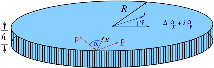
Figure 1: A thin film of $p_{x}+ip_{y}$ superfluid (“2D ³He-A”) confined in a cylindrical geometry with thickness $\mathit{h}\ll\xi$, radius $R\gg\xi$ bounded by specular surfaces which reflect excitations, ${\bf p}\rightarrow\underline{{\bf p}}$.

.2 Bogoliubov-Andreev-Eilenberger

For a thin film of ³He-A, as shown in Fig. 1, the orbital quantization axis is locked normal to the surface of the film, $\hat{\bf l}||\hat{\bf z}$.Ambegaokar et al. (1975) The A-phase also belongs to the class of equal spin pairing (ESP) states with spin structure of the order parameter given by a linear combination of the symmetric Pauli matrices,

$$\Delta_{\alpha\beta}({\bf p})={\bf d}\cdot(i\vec{\sigma}\sigma_{y})_{\alpha\beta}\,\Delta({\bf p})\,,$$ (4)

where $\alpha,\beta$ label the projections of fermion spins of the Cooper pair and ${\bf d}$ is the direction in spin space along which Cooper pairs have zero spin projection. Thus, for ${\bf d}=\hat{\bf z}$ the spin state of the Cooper pairs is given by $i\vec{\sigma}\sigma_{y}\cdot{\bf d}=\sigma_{x}$, which is the triplet state with equal amplitude for the Cooper pairs to be spin polarized along $+\hat{\bf x}$ or $-\hat{\bf x}$: $\mbox{$\displaystyle|\,{\bf d}\,\rangle$}=\frac{1}{\sqrt{2}}\left(\mbox{$\displaystyle|\,\rightrightarrows\,\rangle$}+\mbox{$\displaystyle|\,\leftleftarrows\,\rangle$}\right)$. Spin textures described by spatial variations of the ${\bf d}$ vector are possible; however, in what follows I assume the spin state is fixed by the nuclear dipolar energy which locks the ${\bf d}\,||\,\hat{\bf l}$.Leggett (1975) The bulk A-phase of ³He in 3D has gapless excitations for momenta along the nodal directions, ${\bf p}\,||\pm\,\hat{\bf l}$. Here I consider 2D ³He-A with a cylindrical Fermi surface, (or a set of cylindrical Fermi surfaces generated by dimensional quantization), and an orbital order parameter given by

$$\Delta({\bf p})=\Delta\left(p_{x}+i\,p_{y}\right)/p_{f}\,,$$ (5)

which generates a bulk excitation spectrum that is fully gapped on the Fermi surface.

Near a boundary, or domain wall, the orbital order parameter can deviate from the pure A-phase form. Thus, a more general form of the orbital p-wave order parameter is parametrized by two real amplitudes,

$$\Delta({\bf r},{\bf p})=\Big{(}\Delta_{1}({\bf r})\,p_{x}+i\,\Delta_{2}({\bf r})\,p_{y}\Big{)}/p_{f}\,,$$ (6)

with $\Delta_{1,2}({\bf r})\rightarrow\Delta$ far from a boundary. Inhomogeneous states are described by the Bogoliubov’s equationsVolovik (1988); Kurkijärvi and Rainer (1990); Volovik (1997)

$$\,\left(-\frac{\hbar^{2}}{2m^{*}}\nabla^{2}-\mu\right)u_{\alpha}({\bf r})+\Delta_{\alpha\beta}({\bf r},{\bf p})\,v_{\beta}({\bf r})=\varepsilon\,u_{\alpha}({\bf r})\,,$$ (7)

$$-\left(-\frac{\hbar^{2}}{2m^{*}}\nabla^{2}-\mu\right)v_{\alpha}({\bf r})+\Delta^{{\dagger}}_{\beta\alpha}({\bf r},{\bf p})\,u_{\beta}({\bf r})=\varepsilon\,v_{\alpha}({\bf r})\,.$$ (8)

for the particle ($u_{\alpha}({\bf r})$) and hole ($v_{\alpha}({\bf r})$) wavefunctions. For ${\bf d}={\bf z}$ the Bogoliubov equations reduce to $2\times 2$ equations for Bogoliubov spinors, $\mbox{$\displaystyle|\,\varphi\,\rangle$}=\left(u,v\right)^{\text{T}}$, in Nambu (particle-hole) space,

$$\widehat{{\cal H}}_{\text{B}}\mbox{$\displaystyle|\,\varphi\,\rangle$}=\varepsilon\mbox{$\displaystyle|\,\varphi\,\rangle$}\,,$$ (9)

where $\widehat{{\cal H}}_{\text{B}}$ is the Bogoliubov Hamiltonian expressed in terms of Nambu matrices, ${\widehat{\tau}_{1}},{\widehat{\tau}_{2}},{\widehat{\tau}_{3}}$,

$$\widehat{{\cal H}}_{\text{B}}=\xi({\bf p}){\widehat{\tau}_{3}}+\Delta_{1}({\bf r},{\bf p}){\widehat{\tau}_{1}}+\Delta_{2}({\bf r},{\bf p}){\widehat{\tau}_{2}}\,,$$ (10)

with ${\bf p}=\hbar/i\mbox{\boldmath$\nabla$}$, and the off-diagonal pair potentials interpreted as symmetrized operators,

$$\Delta_{1,2}({\bf r},{\bf p})=\frac{\hbar}{2i}\left(\Delta_{1,2}({\bf r})\,\partial_{x,y}+\partial_{x,y}\,\Delta_{1,2}({\bf r})\right)\,.$$ (11)

The large difference between the Fermi wavelength, $\hbar/p_{f}$, and the size of Cooper pairs, $\xi$, is the basis for Andreev’s quasiclassical approximation to the Bogoliubov equations.Andreev (1964) The expansion is achieved by factoring the fast- and slow spatial variations of the Bogoliubov spinor,

$$\mbox{$\displaystyle|\,\varphi\,\rangle$}=e^{i{\bf p}_{f}\cdot{\bf r}/\hbar}\,\mbox{$\displaystyle|\,\psi_{{\bf p}_{f}}\,\rangle$}\,,$$ (12)

and retaining leading order terms in $\hbar/p_{f}\xi\ll 1$, which yields Andreev’s equation,

$$\widehat{{\cal H}}_{\text{A}}\,\mbox{$\displaystyle|\,\psi_{{\bf p}}\,\rangle$}+i\hbar\,{\bf v}_{{\bf p}}\cdot\mbox{\boldmath$\nabla$}\,\mbox{$\displaystyle|\,\psi_{{\bf p}}\,\rangle$}=0\,.$$ (13)

with operator ${\cal H}_{\text{A}}$ defined by

$$\widehat{{\cal H}}_{\text{A}}=\varepsilon{\widehat{\tau}_{3}}-\widehat{\Delta}({\bf r},{\bf p})\,,$$ (14)

and the Nambu matrix order parameter given is by

$$\widehat{\Delta}({\bf r},{\bf p})=i\sigma_{x}\left({\widehat{\tau}_{1}}\Delta_{2}({\bf r},{\bf p})+{\widehat{\tau}_{2}}\Delta_{1}({\bf r},{\bf p})\right)\,,$$ (15)

where ${\bf p}=p_{f}\hat{p}$ is the Fermi momentum, ${\bf v}_{{\bf p}}=v_{f}\hat{p}$ is the Fermi velocity. The latter defines classical straight-line trajectories for the propagation of wavepackets of Bogoliubov excitations, which are coherent superpositions of particles and holes with amplitudes given by the Andreev-Nambu spinor,

$$\mbox{$\displaystyle|\,\psi_{{\bf p}}\,\rangle$}=\begin{pmatrix}{u}_{{\bf p}}\cr{v}_{{\bf p}}\end{pmatrix}\,.$$ (16)

Andreev’s equation expressed in terms of a row spinor is

$$\mbox{$\displaystyle\langle\,\tilde{\psi}_{{\bf p}}\,|$}\widehat{{\cal H}}_{\text{A}}-i\hbar{\bf v}_{{\bf p}}\cdot\mbox{\boldmath$\nabla$}\,\mbox{$\displaystyle\langle\,\tilde{\psi}_{{\bf p}}\,|$}=0\,,$$ (17)

with the normalization of the Andreev-Nambu spinor given by $\mbox{$\displaystyle\langle\,\tilde{\psi}_{{\bf p}}\,|\,\psi_{{\bf p}}\,\rangle$}=1$. There are two solutions (branches) to Andreev’s equation for a single trajectory defined by ${\bf p}$. For $|\varepsilon|>\Delta$, the two branches are propagating solutions; a particle-like solution, $\displaystyle|\,\psi_{{\bf p}\,+}\,\rangle$, with group velocity ${\bf v}(\varepsilon)||{\bf p}$ and hole-like solution, $\displaystyle|\,\psi_{{\bf p}\,-}\,\rangle$, with reversed group velocity, ${\bf v}(\varepsilon)||-{\bf p}$. For energies within the bulk gap the solutions are exploding and decaying amplitudes along the trajectory, and thus relevant only in the vicinity of boundaries, domain walls, etc.

The product of the particle- and hole amplitudes in Eq. 16,

$$\mathfrak{f}_{\alpha\beta}({\bf r},{\bf p};\varepsilon)={u}_{\alpha}({\bf r},{\bf p};\varepsilon){v}_{\beta}({\bf r},{\bf p};\varepsilon)\,,$$ (18)

is the pair propagator, which determines the spectral composition of the Cooper pair amplitude,

$${\cal F}_{\alpha\beta}({\bf r},{\bf p})=\int d\varepsilon\,f(\varepsilon)\,\,\mathfrak{f}_{\alpha\beta}({\bf r},{\bf p};\varepsilon)\,,$$ (19)

where $f(\varepsilon)=1/(e^{\varepsilon/T}+1)$ is the Fermi distribution. The pair propagator is one component of the Nambu matrix

$$\widehat{\mathfrak{g}}({\bf r},{\bf p};\varepsilon)=\sum_{\mu,\nu}\,g_{\mu\nu}\,\mbox{$\displaystyle|\,\psi_{{\bf p}\mu}\,\rangle$}\mbox{$\displaystyle\langle\,\tilde{\psi}_{{\bf p}\nu}\,|$}\,,$$ (20)

which satisfies Eilenberger’s transport equation,Eilenberger (1968)

$$\left[\widehat{{\cal H}}_{\text{A}}\,,\,\widehat{\mathfrak{g}}({\bf r},{\bf p};\varepsilon)\right]+i\hbar{\bf v}_{{\bf p}}\cdot\mbox{\boldmath$\nabla$}\,\widehat{\mathfrak{g}}({\bf r},{\bf p};\varepsilon)=0\,.$$ (21)

Physical solutions to Eq. 21 must also satisfy Eilenberger’s normalization condition,Eilenberger (1968)

$$\left(\widehat{\mathfrak{g}}({\bf r},{\bf p};\varepsilon)\right)^{2}=-\pi^{2}\widehat{1}\,.$$ (22)

An advantage of Eilenberger’s formulation is that the spectral functions for both quasiparticle and pair excitations are obtained as components of the quasiclassical propagator. For a fixed spin quantization axis, ${\bf d}=\hat{\bf z}$, the off-diagonal components of the propagator describe pure equal-spin pairing correlations. As a result the Nambu propagator can be expressed in the form,

$$\widehat{\mathfrak{g}}^{\text{R}}=\mathfrak{g}^{\text{R}}_{3}{\widehat{\tau}_{3}}+i\sigma_{x}\,\left(\mathfrak{f}^{\text{R}}_{2}{\widehat{\tau}_{1}}-\mathfrak{f}^{\text{R}}_{1}{\widehat{\tau}_{2}}\right)\,.$$ (23)

The superscript refers to the causal (retarded in time) propagator, obtained from Eq. 21 with the shift, $\varepsilon\rightarrow\varepsilon+i0^{+}$. The diagonal propagator in Nambu space, $\mathfrak{g}^{\text{R}}_{3}{\widehat{\tau}_{3}}$, determines the spectral function, or local density of states, for the fermionic excitations with momentum ${\bf p}=p_{f}\hat{p}$,

$${\cal N}({\bf r},{\bf p};\varepsilon)=-\frac{1}{\pi}\mathfrak{Im}\,\,\mathfrak{g}^{\text{R}}_{3}({\bf r},{\bf p};\varepsilon)\,,$$ (24)

while the off-diagonal propagators, $\mathfrak{f}^{\text{R}}_{1}{\widehat{\tau}_{2}}$ and $\mathfrak{f}^{\text{R}}_{2}{\widehat{\tau}_{1}}$, determine the spectral function for the correlated pairs,

$${\cal P}_{1,2}({\bf r},{\bf p};\varepsilon)=-\frac{1}{\pi}\mathfrak{Im}\,\,\mathfrak{f}^{\text{R}}_{1,2}({\bf r},{\bf p};\varepsilon)\,.$$ (25)

These functions determine the mean pair potentials, $\Delta_{1}$ and $\Delta_{2}$, through the BCS self-consistency condition,

$$\Delta_{1,2}({\bf r},{\bf p})=\langle v({\bf p},{\bf p}^{\prime})\int^{+\Omega_{\text{c}}}_{-\Omega_{\text{c}}}d\varepsilon\tanh\left(\frac{\varepsilon}{2T}\right){\cal P}_{1,2}({\bf r},{\bf p}^{\prime};\varepsilon)\rangle_{{\bf p}^{\prime}}\,,$$ (26)

where $\Omega_{c}\ll E_{F}$ is the bandwidth of attraction for the spin-triplet, p-wave pairing interaction, $v({\bf p},{\bf p}^{\prime})$, which is integrated over the occupied states defining the pair spectrum and averaged over the Fermi surface, $\langle\ldots\rangle_{{\bf p}^{\prime}}\equiv\int\,d\Omega_{{\bf p}^{\prime}}/4\pi(\ldots)$.

.3 Chiral Edge State

For a boundary far from other boundaries only single reflections, ${\bf p}\rightarrow\underline{{\bf p}}$, couple the propagators for the incoming (${\bf p}$) and outgoing ($\underline{{\bf p}}$) trajectories. In particular, for the pair of specularly reflected trajectories on the boundary shown in Fig. 1, with radius of curvature large compared to the correlation length, $R\gg\xi$, the solutions for the components of the propagator are (see Appendix I)

$$\mathfrak{f}^{\text{R}}_{1}(x,{\bf p};\varepsilon) = \frac{\pi\Delta_{1}}{\lambda(\varepsilon)}\,\left(1-e^{-2\lambda(\varepsilon)x/v_{x}}\right)\,,$$ (27)

$$\mathfrak{f}^{\text{R}}_{2}(x,{\bf p};\varepsilon) = \frac{\pi\Delta_{2}}{\lambda(\varepsilon)}\,-\frac{\pi\Delta_{1}}{\lambda(\varepsilon)}\,\frac{\Delta_{1}^{2}-(\tilde{\varepsilon}^{\text{R}})^{2}}{\lambda\tilde{\varepsilon}^{\text{R}}-\Delta_{1}\Delta_{2}}\,e^{-2\lambda(\varepsilon)x/v_{x}}\,,$$ (28)

$$\mathfrak{g}^{\text{R}}_{3}(x,{\bf p};\varepsilon) = -\frac{\pi\tilde{\varepsilon}^{\text{R}}}{\lambda(\varepsilon)}+\frac{\pi\Delta_{1}}{\lambda(\varepsilon)}\,\frac{\tilde{\varepsilon}^{\text{R}}\Delta_{1}+\lambda\Delta_{2}}{(\tilde{\varepsilon}^{\text{R}})^{2}-\Delta_{2}^{2}}\,e^{-2\lambda(\varepsilon)x/v_{x}}\,.\qquad$$ (29)

where $v_{x}=v_{f}\cos(\alpha)$ for $-\pi/2<\alpha<\pi/2$ and $x\geq 0$ is the coordinate normal to the boundary as shown in Fig. 1.

Note that the propagator corresponding to Cooper pairs with relative momentum normal to the boundary vanishes at the boundary, $\mathfrak{f}^{\text{R}}_{1}(x=0,{\bf p};\varepsilon)\equiv 0$. De-pairing of the normal amplitude is partially compensated by an increase in the pairing correlations for pairs with relative momenta parallel to the boundary. The origin of this enhancement is the fermionic state, bound to the surface, which appears as a pole in the propagators of Eqs. 28 and 29 at the energies,

$$\varepsilon_{\text{bs}}({\bf p})=-\Delta_{2}({\bf p})=-c\,p_{||}\,.$$ (30)

The surface state disperses with momentum $p_{||}=p_{f}\sin\alpha$ parallel to the surface, $-p_{f}\leq p_{||}\leq+p_{f}$, and $c=\Delta/p_{f}\ll v_{f}$.

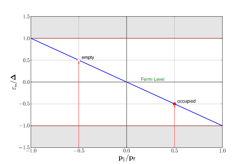
Figure 2: Chiral edge state dispersion, $\varepsilon_{\text{bs}}({\bf p})=-c\,p_{||}$, illustrating the asymmetry in the occupation of pairs of time-reversed states.

The important feature of the spectrum of surface fermions, shown in Fig. 2, is that there is no branch with the opposite phase velocity. The spectrum describes Weyl or chiral fermions.Volovik (1997)^, For each pair of time-reversed fermions the state with $+p_{||}$ is occupied while its time-reversed partner with momentum $-p_{||}$ is empty. As a result the pairs of surface states generate a net mass or charge current. This asymmetry in the occupation of the surface spectrum is a reflection of the chirality of the ground state order parameter and specular reflection at the boundary which preserves translation symmetry locally along the boundary. The absence of a branch of fermions with energy $\varepsilon_{+}({\bf p}_{||})=+\Delta_{2}({\bf p})$ is demonstrated by evaluating the residue of $\mathfrak{g}^{\text{R}}_{3}(x,{\bf p};\varepsilon)$ at the apparent pole, $\varepsilon_{+}$: $\mbox{Res}\,\mathfrak{g}^{\text{R}}_{3}(x,{\bf p};\varepsilon)|_{\varepsilon_{+}}\equiv 0$. For energies in the vicinity of the bound-state pole, $|\varepsilon-\varepsilon_{\text{bs}}|\ll|\Delta|$, the quasiparticle propagator reduces to

$$\mathfrak{g}^{\text{R}}_{\text{bs}}(x,{\bf p};\varepsilon)=\frac{\pi|\Delta_{1}({\bf p})|}{\varepsilon+i\gamma-\varepsilon_{\text{bs}}({\bf p})}\,e^{-2\Delta\,x/v_{f}}\,,$$ (31)

where I include the line-width, $\gamma\ll\Delta$, of the surface state due to weak disorder. For $\gamma\rightarrow 0^{+}$ the states are sharp and the spectral function consists of delta functions at $\varepsilon_{\text{bs}}({\bf p})$,

$${\cal N}_{\text{bs}}(x,{\bf p};\varepsilon)=\pi|\Delta_{1}({\bf p})|\,e^{-2\Delta\,x/v_{f}}\,\delta(\varepsilon-\varepsilon_{\text{bs}}({\bf p}))\,.$$ (32)

The spectral weight is maximum for trajectories at normal incidence and vanishes for grazing incidence. Note that every edge state is confined to the surface on the length scale

$$\xi_{\text{$\Delta$}}=\hbar v_{f}/2\Delta\,,$$ (33)

independent of momentum ${\bf p}_{||}$, and of order the Cooper pair size, $\xi_{\text{$\Delta$}}=\hbar v_{f}/2\Delta\simeq 1.6\,\xi$.

.4 Spectral Current Density

The spectral current density is defined as the local density of current carrying states in the energy interval $(\varepsilon,\varepsilon+d\varepsilon)$ for states with momentum ${\bf p}$,

$${\cal J}(x,{\bf p};\varepsilon)=2N_{f}{\bf v}_{{\bf p}}\,\left[{\cal N}_{\text{in}}(x,{\bf p};\varepsilon)-{\cal N}_{\text{in}}(x,{\bf p}^{\prime};\varepsilon)\right]\,,$$ (34)

where ${\cal N}_{\text{in}}(x,{\bf p};\varepsilon)$ is the spectral function calculated for the incident trajectory with momentum ${\bf p}$, $N_{f}$ is the normal-state density of states at the Fermi level for one spin, and ${\bf p}$ and ${\bf p}^{\prime}$ define the pair of time-reversed incident trajectories shown in Fig. 3a, for which ${\bf v}_{\underline{{\bf p}}^{\prime}}=-{\bf v}_{{\bf p}}$.

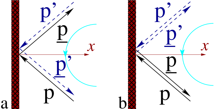
Figure 3: a) Time-reversed trajectory pairs that define the spectral current density, ${\cal J}(x,{\bf p};\varepsilon)$, for specular reflections. b) Retro-reflections are time-reversed partners for any incident angle. The chirality of the bulk order parameter is indicated by the direction of the arc.

The resulting local current density is obtained by thermally occupying the spectrum and integrating over all incoming trajectories,

$${\bf j}(x)=\int_{\text{in}}\frac{d\Omega_{{\bf p}}}{4\pi}\int_{-\infty}^{+\infty}\,d\varepsilon\,f(\varepsilon)\,{\cal J}(x,{\bf p};\varepsilon)\,,$$ (35)

where $f(\varepsilon)=1/(e^{\varepsilon/T}+1)$ is the Fermi distribution.

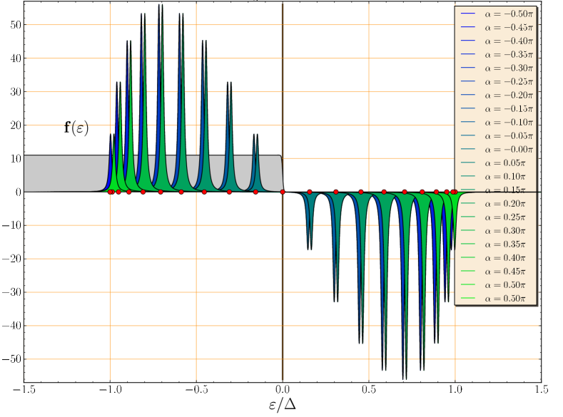
Figure 4: Spectral current density ${\cal J}_{y}$ for $x=0$ as a function of $p_{||}=p_{f}\sin\alpha$ for linewidth $\gamma=0.025\Delta$. States with $\pm p_{||}$ are slightly offset to show the contributions to the current from time-reversed pairs.

The spectral current density for the bound-state spectrum obtained from Eqs. 31 and 34 is shown in Fig. 4 for the full range of incident trajectories. Note that time-reversed states, incident angles $\alpha$ and $-\alpha$, add coherently to the spectral current density. Thus, the net current density parallel to the boundary carried by the surface bound states is given by

$$j_{y}^{\text{bs}}(x) = I(\Delta/T)\times N_{f}\,v_{f}\,\Delta\,e^{-x/\xi_{\text{$\Delta$}}}\,,$$ (36)

where the integration over the spectrum reduces to

$$I=\int_{-1}^{+1}\,du\,u\,\tanh(\Delta\,u/2T)=\Bigg{\{}\begin{array}[]{ll}1&\,,\,T\rightarrow 0\cr\frac{\Delta(T)}{12T_{c}}&\,,\,T\rightarrow T_{c}\end{array}\,.$$ (39)

Note that near the transition the magnitude of the current decreases as $j_{y}\sim\Delta^{2}(T)/T_{c}\sim(1-T/T_{c})$, but also penetrates deeper into the bulk as $\xi_{\text{$\Delta$}}=\hbar v_{f}/2\Delta(T)\sim(1-T/T_{c})^{-\frac{1}{2}}$.

.5 Edge Currents and Angular Momentum

Mass currents confined near the boundary (“edge currents”) generate macroscopic angular momentum. For a Galilean invariant system such as liquid ³He the mass current density is obtained from the spectral current density in Eq. 34 by the replacement ${\bf v}_{{\bf p}}\rightarrow m^{*}{\bf v}_{{\bf p}}={\bf p}$, where $m^{*}$ is the quasiparticle effective mass, ${\bf p}=p_{f}\hat{\bf p}$ is the Fermi momentum. In addition, $v_{f}$, $p_{f}$ and the normal-state density of states, $N_{f}$, determine the particle number density, which for a 2D Fermi surface gives $n\equiv N/V=N_{f}\,p_{f}\,v_{f}$.

For a chiral p-wave superfluid confined within a thin cylindrical vessel of radius $R$ and height $h$ in the 2D limit, $h\ll\xi_{\text{$\Delta$}}\ll R$, the angular momentum relative to the $z$-axis is determined by the radial moment of the azimuthal component of the mass current density, $g_{\varphi}({\bf r})$,

$$L_{z}=\int_{\text{V}}d^{3}r\,\left[r\,g_{\varphi}({\bf r})\right]\,.$$ (40)

For $R\gg\xi_{\text{$\Delta$}}$ we can neglect the curvature of the surface, in which case the azimuthal mass current is given by the tangential component of the boundary current calculated from Eq. 35. Thus, the bound-state contribution to $L_{z}$ at $T=0$ obtained from Eqs. 40 and 36, with $v_{f}\rightarrow p_{f}$ becomes,

$$L_{z}^{\text{bs}} = N_{f}\,p_{f}\,\Delta\,\times\,2\pi\,h\int_{0}^{R}r^{2}\,dr\,e^{-(R-r)/\xi_{\text{$\Delta$}}}=N\,\hbar\,,$$ (41)

which is a factor of two larger than that predicted by Ishikawa Ishikawa (1977) and McClure and TakagiMcClure and Takagi (1979) based on the real-space N-particle wave function of Eq. 1. Finite size corrections from Eq. 41 are negligible - of order $\xi_{\text{$\Delta$}}/R\lll 1$. As Stone and Roy pointed out the discrepancy is resolved by including the contribution to $L_{z}$ from the states comprising the continuum spectrum.Stone and Roy (2004) Below I analyze the continuum contributions to the edge current and ground state angular momentum. In particular, I show that there are two contributions to the continuum spectral current density: (i) an isolated scattering resonance that exactly cancels the bound-state contribution to the edge current for each value of ${\bf p}$ and (ii) a non-resonant response of the bound continuum that accounts exactly for the MT result of $L_{z}=(N/2)\hbar$.

The energy range $\varepsilon<-\Delta$ constitutes the bound continuum, while the range $\varepsilon>+\Delta$ represents excitations above the gap. At finite temperatures sub-gap surface excited states $0<\varepsilon<\Delta$ also play an important role. The spectral weight associated with the continuum spectrum is modified near the boundary. For $|\varepsilon|>\Delta$, $\lambda(\varepsilon)=i\,\mbox{sgn}(\varepsilon)\sqrt{\varepsilon^{2}-\Delta^{2}}$ and the spectral function becomes,

$${\cal N}_{\text{c}}(x,{\bf p};\varepsilon) = \frac{|\varepsilon|}{\sqrt{\varepsilon^{2}-\Delta^{2}}}$$

$$- \frac{|\varepsilon|}{\sqrt{\varepsilon^{2}-\Delta^{2}}}\frac{\Delta^{2}_{1}({\bf p})}{\varepsilon^{2}-\Delta^{2}_{2}({\bf p})}\cos(2\sqrt{\varepsilon^{2}-\Delta^{2}}\,x/v_{x})$$

$$- \mbox{sgn}(\varepsilon)\,\left(\frac{\Delta_{1}({\bf p})\Delta_{2}({\bf p})}{\varepsilon^{2}-\Delta^{2}_{2}({\bf p})}\right)\sin(2\sqrt{\varepsilon^{2}-\Delta^{2}}\,x/v_{x})\,.$$

The first term is the bulk continuum spectrum, while the corrections to the continuum spectrum are given by second and third lines in Eq. .5. The third term is odd under either $\varepsilon\rightarrow-\varepsilon$ or ${\bf p}\rightarrow-{\bf p}$, and thus gives a non-vanishing contribution to the spectral current density,

$${\cal J}_{\text{c}}(x,{\bf p};\varepsilon) = -2N_{f}{\bf v}_{{\bf p}}\,\mbox{sgn}(\varepsilon)\left(\frac{\Delta_{1}({\bf p})\Delta_{2}({\bf p})}{\varepsilon^{2}-\Delta^{2}_{2}({\bf p})}\right)$$ (43)

$$\times \sin(2\sqrt{\varepsilon^{2}-\Delta^{2}}\,x/v_{x})$$

Note that for fixed energy $\varepsilon$ and momentum ${\bf p}$ the effect of surface scattering on the continuum spectrum is large and propagates into the bulk. Thus, it is not a priori clear that the current is confined to the surface. However, the wavelength of the disturbance is given by the Tomasch wavelength for a specific trajectory,

$$\lambda_{\text{T}}({\bf p},\varepsilon)=\frac{\pi\hbar v_{f}\hat{p}_{x}}{\sqrt{\varepsilon^{2}-\Delta^{2}}}\,.$$ (44)

The net current parallel to the boundary is given by the sum over all incident trajectories,

$$j_{y}^{\text{c}}(x)=2N_{f}v_{f}\,\int_{-\pi/2}^{+\pi/2}\,\frac{d\alpha}{\pi}\,\hat{p}_{y}\,\Delta_{1}({\bf p})\Delta_{2}({\bf p})\times J({\bf p})\,,$$ (45)

where $J({\bf p})$ is given by

$$J({\bf p})=\int_{\Delta}^{\infty}\,d\varepsilon\frac{\tanh(\varepsilon/2T)}{\varepsilon^{2}-\Delta^{2}_{2}({\bf p})}\times\sin(2\sqrt{\varepsilon^{2}-\Delta^{2}}\,x/v_{x})\,.$$ (46)

The integration over the spectral current density leads to phase cancellation away from the boundary, and a net current that is confined to the edge. Although the integration is over the continuum spectrum, the chiral edge state nevertheless modifies the current carried by the continuum states. Trajectories near grazing incidence give a large enhancement to the kernel $J({\bf p})$ coming from the off-resonant bound state. The kernel is weighted by the product $\hat{p}_{y}\,\Delta_{1}({\bf p})\Delta_{2}({\bf p})$, which is peaked near $\alpha\approx\pm 55^{o}$.

At zero temperature the kernel is evaluated by transforming to an integration over the radial momentum $p$, or equivalently $\xi=v_{f}(p-p_{f})$ with $\xi^{2}=\varepsilon^{2}-\Delta^{2}$,

$$J({\bf p})=\frac{\mbox{\small 1}}{\mbox{\small 2}}\mathfrak{Im}\,\,\int_{{\cal C}_{\text{R}}}\,d\xi\frac{\xi}{(\xi^{2}+\Delta_{1}^{2})\sqrt{\xi^{2}+\Delta^{2}}}\times e^{2i\xi\,x/v_{x}}\,.$$ (47)

The singularities shown in the upper half of the complex $\xi$-plane determine the continuum current response. In particular, the integral along the real axis is transformed to an integral around the pole at $i|\Delta_{1}|$ and the branch cut from $i\Delta$ to $i\,\infty$: $J_{{\cal C}_{\text{R}}}=J_{{\cal C}_{\text{1}}}+J_{{\cal C}_{\text{2}}}$.

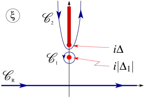
Figure 5: Integration in the complex $\xi$ plane. Integration along the real axis (${\cal C}_{\text{R}}$) is transformed into the sum of an integral around the isolated pole at $i|\Delta_{1}|$ and the branch cut along the imaginary $\xi$-axis.

The pole at $\xi=i|\Delta_{1}|$ is an isolated resonance that gives a contribution to the continuum current that is confined to the boundary on the length scale $\xi_{\text{$\Delta$}}$,

$$J_{{\cal C}_{\text{1}}}=\frac{\pi}{2|\Delta_{2}({\bf p})|}\,e^{-x/\xi_{\text{$\Delta$}}}\,.$$ (48)

The current generated by this resonance exactly cancels the bound-state edge current and bound-state contribution to the angular momentum,

$$L_{z}^{{\cal C}_{\text{1}}}=\int_{\text{V}}d^{2}r\,\left[r\,g_{\varphi}^{{\cal C}_{\text{1}}}({\bf r})\right]=-N\hbar\,.$$ (49)

Thus, the ground-state current and angular momentum come entirely from the non-resonant contribution to the continuum spectrum defined by the branch cut ${\cal C}_{\text{2}}$ which evaluates to

$$J_{{\cal C}_{\text{2}}}=-\int_{0}^{\infty}\frac{d\varepsilon}{\varepsilon^{2}+|\Delta_{2}({\bf p})|^{2}}\,e^{-2\sqrt{\varepsilon^{2}+\Delta^{2}}\,x/v_{x}}\,.$$ (50)

The current density is then given by

$$j_{y}^{{\cal C}_{\text{2}}}(x) = 2N_{f}v_{f}\,\int_{-\pi/2}^{+\pi/2}\,\frac{d\alpha}{\pi}\,\hat{p}_{y}\,|\Delta_{1}({\bf p})|\Delta_{2}({\bf p})$$ (51)

$$\times \int_{0}^{\infty}\frac{d\varepsilon}{\varepsilon^{2}+|\Delta_{2}({\bf p})|^{2}}\,e^{-2\sqrt{\varepsilon^{2}+\Delta^{2}}\,x/v_{x}}\,,$$

which is confined to the edge, but in contrast to the bound-state and resonance terms, there is not a single confinement length, but rather a weighted average of exponential confinement on length scales $\pi\hbar v_{f}\,\cos\alpha/\Delta$. For this reason an analytic expression for the net current density analogous to Eq. 36 does not appear possible. However, the total edge current and ground state angular momentum can be computed by first carrying out the integration over the region of the edge current. In the limit $R\gg\xi_{\text{$\Delta$}}$ the resulting ground-state angular momentum reduces to the following integration over the continuum spectrum,

$$L_{z}^{{\cal C}_{\text{2}}}=N\hbar \times \frac{2}{\pi}\int_{-\pi/2}^{+\pi/2}\,d\alpha\,p_{x}\,p_{y}\,\Delta_{1}({\bf p})\Delta_{2}({\bf p})$$

$$\times \int_{0}^{\infty}\frac{d\varepsilon}{(\varepsilon^{2}+|\Delta_{2}({\bf p})|^{2})\sqrt{\varepsilon^{2}+\Delta^{2}}}\,,$$

which evaluates to (see Appendix II)

$$L_{z}^{{\cal C}_{\text{2}}}=\frac{N}{2}\hbar\,.$$ (53)

Thus, IshikawaIshikawa (1977), McClure and TakagiMcClure and Takagi (1979) and Stone and Roy’sStone and Roy (2004) results are recovered from the continuum response to the formation of the chiral edge state.

.6 Temperature Dependence of $L_{z}$

For $T\neq 0$ thermal excitations out of the ground state lead to a reduction of the order parameter $\Delta(T)$, the edge current and angular momentum. The latter can be expressed as

$$L_{z}(T)=\frac{N}{2}\hbar\,\times{\cal Y}_{\text{$L_{z}$}}(T)\,,$$ (54)

where ${\cal Y}_{\text{$L_{z}$}}(T)\rightarrow 1$ for $T\rightarrow 0$, vanishes for $T\rightarrow T_{c}$, and can be calculated from the edge current at finite temperature.

Calculations of the temperature dependence of the angular momentum for ³He-A were carried out by T. Kita on the basis of numerical solutions to the Bogoliubov equations for mesoscopic cylindrical (3D) geometries with dimensions $R\sim 4h\sim 2\xi$. Kita showed that ${\cal Y}_{\text{$L_{z}$}}(T)$ decreases rapidly for $T\gtrsim 0$, indicating that there are low-lying excitations that are thermally populated even at low temperatures which reduce the ground-state angular momentum. Based on his numerical results (Fig. 2a of Ref. Kita, 1998), Kita conjectured that the temperature dependence of ${\cal Y}_{\text{$L_{z}$}}(T)$ resulted from the excitations responsible for the suppression of the superfluid density $\rho_{s,||}(T)$ of bulk ³He-A corresponding to superflow along the nodal direction for the 3D chiral p-wave superfluid. For 3D bulk superfluid ³He-A the stiffness for ${\bf p}_{s}||\,\hat{\bf l}$ is strongly suppressed at finite temperature compared to the stiffness for superflow perpendicular to the nodal direction, i.e. $\rho_{s,\perp}\gg\rho_{s,||}$. However, as I discuss below, the softness of the angular momentum response function ${\cal Y}_{\text{$L_{z}$}}(T)$ that Kita found numerically, including its near equality with $\rho_{s,||}(T)$ for the 3D A-phase, is also present in the 2D limit in which the chiral p-wave superfluid is fully gapped.

For $T\neq 0$ the edge current is determined by the continuum contribution to the spectrum defined in Eq. 45 with,

$$J({\bf p})=\frac{\mbox{\small 1}}{\mbox{\small 2}}\mathfrak{Im}\,\,\int_{{\cal C}_{\text{R}}}\,d\xi\frac{\xi\,\tanh(\sqrt{\xi^{2}+\Delta^{2}}/2T)}{(\xi^{2}+\Delta_{1}^{2})\sqrt{\xi^{2}+\Delta^{2}}}\times e^{2i\xi\,x/v_{x}}\,.$$ (55)

As is the case for $T=0$, the resonant contribution to the continuum current density coming from the isolated pole at $\xi=+i|\Delta_{1}|$ exactly cancels the bound state contribution. However, the total edge current and angular momentum, which at $T=0$ is calculated from the branch cut in Fig. 5, now results from the sum of contributions from a discrete set of poles at the complex momenta defined by

$$\xi_{n}=i\sqrt{\varepsilon_{n}^{2}+\Delta^{2}}\,,$$ (56)

where $\varepsilon_{n}=(2n+1)\pi T$, $n=0,\pm 1,\pm 2,\ldots$, are the fermion Matsubara frequencies. The resulting edge current density is given by

$$j_{y}^{{\cal C}_{\text{2}}}(x) = 2N_{f}v_{f}\,\int_{-\pi/2}^{+\pi/2}\,\frac{d\alpha}{\pi}\,p_{y}\,|\Delta_{1}({\bf p})|\Delta_{2}({\bf p})$$ (57)

$$\times \pi T\sum_{\varepsilon_{n}}\frac{1}{\epsilon_{n}^{2}+|\Delta_{2}({\bf p})|^{2}}\,e^{-2\sqrt{\epsilon_{n}^{2}+\Delta^{2}}\,x/v_{x}}\,.$$

Multiple confinement scales are manifest in Eq. 57. The total surface current obtained by integrating over the boundary region determines the equilibrium angular momentum generated by these edge currents,

$${\cal Y}_{\text{$L_{z}$}}(T)=\frac{8}{\pi}\int_{0}^{1}dx\,(1-x^{2})^{\frac{\mbox{\tiny 1}}{\mbox{\tiny 2}}}\pi T\sum_{\varepsilon_{n}}\frac{\Delta^{2}\,x^{2}}{\varepsilon_{n}^{2}+\Delta^{2}x^{2}}\frac{1}{\sqrt{\varepsilon_{n}^{2}+\Delta^{2}}}\,,$$ (58)

where $x=\hat{p}_{y}=\sin\alpha$. Figure 6 shows the temperature dependence of the equilibrium angular momentum, ${\cal Y}_{\text{$L_{z}$}}(T)$, calculated from Eq. 58. Also shown for comparison is the bulk excitation gap and superfluid stiffness for both 2D and 3D chiral p-wave states. Note that the temperature dependence of the angular momentum is much softer than the bulk superfluid stiffness for the gapless 2D phase.

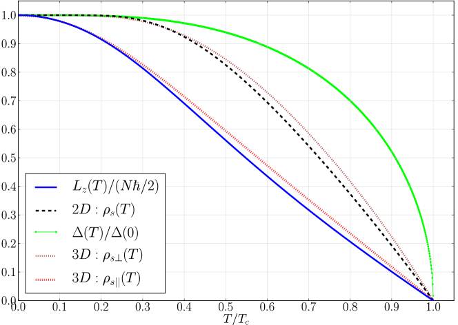
Figure 6: Temperature dependence of the angular momentum, $L_{z}(T)$, for the 2D chiral p-wave superfluid (–). Also shown is the superfluid stiffness (–) and the bulk gap (–) for the fully gapped 2D chiral p-wave state. Shown for comparison are the two components of the superfluid stiffness for the 3D chiral, p-wave superfluid phase (³He-A) - $\rho_{s,||}$ for ${\bf p}_{s}||\hat{\bf l}$ (–) and $\rho_{s,\perp}$ for ${\bf p}_{s}\perp\hat{\bf l}$ (–).

Just as Kita found for his 3D mesoscopic geometry, the temperature dependence of $L_{z}(T)$ for the fully gapped 2D phase is nearly identical to the superfluid stiffness for superflow parallel to the nodal direction for the 3D phase. However, the reasons for the rapid suppression of $L_{z}(T)$ and $\rho_{s,||}(T)$ are of different physical origin. For the bulk 3D phase $\rho_{s,||}(T)$ is strongly reduced compared to $\rho_{s,\perp}(T)$ due to the backflow current carried by the nodal excitations when ${\bf p}_{s}||\,\hat{\bf l}$.Xu et al. (1995) By contrast, for the fully gapped 2D chiral phase there are low-energy backflow surface currents for $0<\varepsilon<\Delta$ that reduce the edge current when thermally populated (cf Fig. 4). The presence of low-energy surface excitations is also evident in the spectral sums that define the edge current and angular momentum in Eqs. 57-58.

.7 Robustness of the Edge Currents

The result of Ishikawa,Ishikawa (1977) and McClure and Takagi,McClure and Takagi (1979), for the ground-state angular momentum is based a geometry with cylindrical symmetry, a chiral p-wave order parameter and many-body wave function that is an eigenfunction of the angular momentum operator and two-particle wave functions that vanish at the boundary. The analysis presented above relies on the formation of edge states by boundary scattering in the presence of a chiral order parameter. The resulting chiral edge states, and their dispersion relation shown in Fig. 2, play a key role in generating the edge current carried by the continuum states and the resulting ground-state angular momentum of $(N/2)\hbar$. One can ask “how robust are these results to boundary conditions, geometry and topology?”

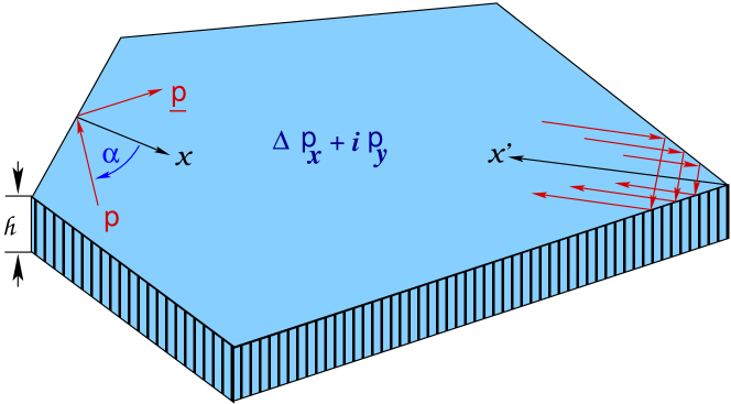
Figure 7: A thin film ($h\ll\xi$) of $p_{x}+ip_{y}$ superfluid (“2D ³He-A”) confined in a non-cylindrical geometry with area ${\cal A}\ggg\xi^{2}$ bounded in the $x-y$ plane by specular surfaces. Double reflections are important in determining the surface spectrum and edge current near a corner.

For example, consider the spectrum, edge currents and ground-state angular momentum for a geometry such as that shown in Fig. 7. There are two classes of trajectories that determine the local spectral current density. Far from a corner ($\approx 5\xi$) trajectories with a single reflection determine the local surface spectrum, and for specular reflections we obtain the chiral edge states and the local edge currents of Eqs. 30 and 51. However, near a corner the sharp change in curvature leads to double reflections as shown in Fig. 7. These double reflections dramatically alter the local excitation spectrum. They are also essential for enforcing current conservation near the corner, and they provide the mechanism for the edge currents to “turn the corner” and maintain continuity of the current circulating near the boundary. Furthermore, since the double reflections are relevant only for incident trajectories within a few coherence lengths of a corner the ground-state angular momentum measured from the center of mass of the film is given by $(N/2)\hbar$ for a finite number of corners, with corrections that are of order $\xi/\bar{R}\lll 1$, where $\bar{R}$ is the minimum linear dimension of the film.

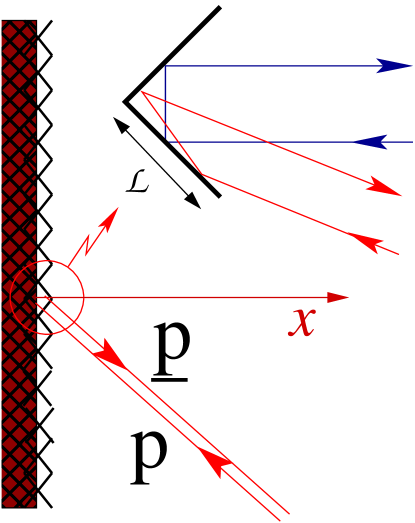
Figure 8: Mesoscopic facets of dimension $\hbar/p_{f}\ll{\cal L}\ll\xi$ are retro-reflectors of quasiparticles.

This example also indicates how non-specular scattering can dramatically alter the surface spectrum, reduce or even eliminate the edge currents. To illustrate the effect non-specular scattering consider a surface that is facetted with mesoscopic mirror surfaces that are large compared to the Fermi wavelength, but small compared to the coherence length, $a\ll{\cal L}\ll\xi$, and oriented at right angles to one another as shown in Fig. 8. Such a surface is a retro-reflector analogous to optical retro-reflectors constructed from dense packing of corner reflectors.Barrett and Jacobs (1979) Note that a retro-reflecting surface does not break time-inversion symmetry or reflection symmetry in a plane containing the normal to the surface, but translational invariance is broken on short-wavelength scales, ${\cal L}\ll\xi$. As a result, retro-reflection can dramatically modify the spectrum of edge states. In the limit of perfect retro-reflection - i.e. retro-reflection of all incident trajectories - the spectrum of edge states is obtained by an analogous calculation to that of perfect specular reflection since every incident trajectory is paired with a single reflected trajectory. In particular, the quasiparticle propagator, and the corresponding bound-state spectral function, are given by (see Appendix I)

$$\mathfrak{g}^{\text{R}}_{3}(x,{\bf p};\varepsilon) = -\frac{\pi\tilde{\varepsilon}^{\text{R}}}{\lambda(\varepsilon)}+\frac{\pi\Delta^{2}}{\lambda(\varepsilon)\tilde{\varepsilon}^{\text{R}}}\,\,e^{-2\lambda(\varepsilon)x/v_{x}}\,,$$ (59)

$${\cal N}_{\text{bs}}(x,{\bf p};\varepsilon) = \pi|\Delta|\,e^{-2\Delta\,x/v_{x}}\,\delta(\varepsilon)\,.$$ (60)

In place of the chiral branch of edge states for perfect specular reflection (Fig. 2), perfect retro-reflection leads to an edge state at the Fermi level, $\varepsilon_{\text{bs}}({\bf p})=0$, i.e. a zero-mode for every incident trajectory, ${\bf p}$. These modes do not carry current, nor do they generate continuum currents. Indeed the spectral current density (Eq. 34) vanishes identically, and thus the ground-state angular momentum resulting from the edge states vanishes as well.

The spectrum of zero-modes is also inferred from the observation that $\Delta(\underline{{\bf p}},x)=-\Delta({\bf p},x)$ for any pair ($\underline{{\bf p}},{\bf p})$ of retro-reflected trajectories. Thus, Andreev’s equation for a pair of retro-reflected trajectories is equivalent to Dirac fermions in 1D coupled to a scalar field $\varphi(z)=\Delta\,\mbox{sgn}(z)$ ($z$ being the coordinate measured along the classical trajectory), which has the well-known Jackiw-Rebbi zero-mode bound to the domain wall at $z=0$.Jackiw and Rebbi (1976)

However, the zero modes generated by retro-reflection and a chiral p-wave order parameter are fragile and unprotected from small perturbations. For an imperfect retro-reflecting surface some incident trajectories will be reflected forward and generate edge currents and a ground-state angular momentum with a magnitude in proportion to the probability for forward reflection. Thus, depending on the distribution of trajectories with forward vs. retro-reflection the resulting ground-state angular momentum will generally be less than $(N/2)\hbar$, and may take on any value in the range, $L_{z}^{\text{min}}\lesssim L_{z}\leq(N/2)\hbar$, with the lower limit set by the intrinsic angular momentum,Volovik (1975); Cross (1977); Balatsky and Mineev (1985)

$$L_{z}^{\text{min}}=(N/2)\hbar\times\frac{1}{4}\,\left(\Delta/E_{f}\right)^{2}\ln(E_{f}/\Delta)\,.$$ (61)

For ³He-A confined by the walls of an experimental cell a realistic estimate for $L_{z}$ is likely below $(N/2)\hbar$, but much larger than the intrinsic limit, and determined by the mean fraction $f$ of forward reflections by the boundary, i.e. $\mbox{sgn}(p_{y})=\mbox{sgn}(\underline{p}_{y}$),

$$L_{z}=f\,\times\,(N/2)\hbar\,,$$ (62)

with $f^{\text{min}}\leq f\leq 1$. The sensitivity of the ground-state angular momentum to retro-reflection is at first sight in conflict with the result of McClure and Takagi (MT). However, the MT boundary condition does not account for retro-reflection on mesoscopic scales because it assumes perfect cylindrical symmetry on the atomic scale. This result highlights the fact that spectrum of edge states, currents and the ground-state angular momentum is sensitive to surface scattering on all scales from several coherence lengths down to the atomic scale.

Figure 9: A thin film of chiral p-wave superfluid (“2D ³He-A”) with $\mathit{h}\ll\xi$, inner and outer radii $R_{2}$, $R_{1}$ and area ${\cal A}=\pi(R_{1}^{2}-R_{2}^{2})$ bounded by specular surfaces which reflect quasiparticles ${\bf p}\rightarrow\underline{{\bf p}}={\bf p}-2\hat{\bf x}(\hat{\bf x}\cdot{\bf p})$. For $R_{1},R_{2},\,R_{1}-R_{2}\gg\xi$ only single reflections are relevant to determining the surface spectrum and edgecurrents on the inner and outer boundaries.

.8 Toroidal Geometry

The combination of geometry and surface boundary conditions can lead to dramatically different results for the ground-state angular momentum of a chiral p-wave superfluid. Consider the toroidal geometry shown in Fig. 9 in which the superfluid is confined between inner and outer baoundaries with radii $R_{2}$ and $R_{1}$, respectively. I assume both radii are large compared to the confinement scale of the chiral edge currents, and that the edge states on the inner and outer boundaries are well separated; i.e. $R_{1},R_{2},R_{1}-R_{2}\gg\xi_{\text{$\Delta$}}$. The ground state angular momentum is given the radial moment of the mass current density in Eq. 40, which in these limits is determined by the mass sheet current on the inner and outer boundaries, $K_{2}$ and $K_{1}$, respectively,

$$L_{z}=2\pi\,h\,\left(K_{1}\,R_{1}^{2}+K_{2}\,R_{2}^{2}\right)\,.$$ (63)

At $T=0$ the magnitude of the mass sheet current (with units of “action/volume”) for a specular boundary is obtained from Eq. 51 with $v_{f}\rightarrow p_{f}$, and evaluates to

$$K=\int_{0}^{\infty}dx\,g_{\varphi}(x)=\frac{1}{4}\,N_{f}\,v_{f}\,p_{f}\,\hbar=\frac{1}{4}\,n\,\hbar\,.$$ (64)

For perfect specular reflection on both boundaries we obtain edge currents of equal magnitude flowing in opposite directions, $K_{1}=-K_{2}=K$, as indicated in Fig. 9, and thus once again the MT result for the ground-state angular momentum,

$$L_{z}=2\pi\,h\,\left(R_{1}^{2}-R_{2}^{2}\right)\,\frac{1}{4}\,n\,\hbar=\frac{N}{2}\hbar\,.$$ (65)

Note that the counter-propagating edge currents conspire to give a ground-state angular momentum, in units of $\hbar/2$, that is extensive and proportional to the volume, or total number of particles. If the boundary is not perfectly specular then the corresponding sheet current is reduced by the suppression of the edge currents by retro-reflection: $K_{f}=f\times\frac{1}{4}\,n\,\hbar$, with suppression factor $0<f<1$.

For the toroidal geometry the inner and outer boundaries may have different degrees of specularity, i.e. $K_{1}=f_{1}\,K$ and $K_{2}=-f_{2}\,K$ with $f_{1}\neq f_{2}$. The generalization of Eq. 65 is

$$L_{z}=\frac{N}{2}\hbar\,\times\left(\frac{f_{1}-r\,f_{2}}{1-r}\right)\,,$$ (66)

where $1<r\leq 0$ is the ratio of the radii, $r=R_{2}/R_{1}$. The asymmetry in the counter-propagating edge currents now leads to a ground-state angular momentum that no longer scales with the volume. Two cases highlight the non-extensive property of $L_{z}$, and its sensitivity to the asymmetry in the edge currents on different boundaries.

For perfect specular reflection on the outer boundary, $f_{1}=1$, and perfect retro-reflection on the inner boundary, $f_{2}=0$, the resulting ground-state angular momentum

$$L_{z}=\frac{N}{2}\hbar\,\times\left(\frac{1}{1-r}\right)\,,$$ (67)

can be much larger than the MT result $(N/2)\hbar$ for $1-r\ll 1$.

Equally dramatic would be to engineer the outer boundary to be retro-reflecting, $f_{1}=0$, and the inner boundary to be specular reflecting, $f_{2}=1$. In this limit only the counter-circulating current on the inner boundary survives, which leads to a ground-state angular momentum that is opposite to the chirality of the Cooper pairs,

$$L_{z}=\frac{N}{2}\hbar\,\times\left(\frac{-r}{1-r}\right)\,.$$ (68)

This reversal of the ground-state angular momentum for a toroidal geometry would provide both be a signature of the broken time-reversal symmetry of the ground state of superfluid ³He-A, and also establish its origin as the edge current from the inner boundary.

I Appendix: Boundary Solutions

Using the representation for $\widehat{\mathfrak{g}}^{\text{R}}$ in Eq. 23, Eilenberger’s equation can be expressed as coupled equations for the quasiparticle and pair propagators in a three-dimensional vector space,

$$\frac{1}{2}\,{\bf v}_{{\bf p}}\cdot\mbox{\boldmath$\nabla$}\mbox{$\displaystyle|\,g\,\rangle$}=\widehat{M}\mbox{$\displaystyle|\,g\,\rangle$}\,,$$ (69)

with

$$\mbox{$\displaystyle|\,g\,\rangle$}\equiv\begin{pmatrix}\mathfrak{f}^{\text{R}}_{1}\cr\mathfrak{f}^{\text{R}}_{2}\cr\mathfrak{g}^{\text{R}}_{3}\end{pmatrix}\,,\quad\widehat{M}=\begin{pmatrix}0&\tilde{\varepsilon}^{R}&\Delta_{2}\cr-\tilde{\varepsilon}^{R}&0&-\Delta_{1}\cr\Delta_{2}&-\Delta_{1}&0\end{pmatrix}$$ (70)

For a uniform order parameter defined by trajectory ${\bf p}$ we express $\displaystyle|\,g\,\rangle$ in terms of the eigenvectors of $\widehat{M}$, $\widehat{M}\mbox{$\displaystyle|\,\mu\,\rangle$}=\mu\mbox{$\displaystyle|\,\mu\,\rangle$}$. The eigenvector with $\mu=0$,

$$\mbox{$\displaystyle|\,0;{\bf p}\,\rangle$}=\frac{1}{\lambda({\bf p},\varepsilon)}\begin{pmatrix}-\Delta_{1}({\bf p})\cr-\Delta_{2}({\bf p})\cr+\tilde{\varepsilon}^{\text{R}}\end{pmatrix}\,,$$ (71)

generates the bulk equilibrium propagator,

$$\widehat{\mathfrak{g}}^{\text{R}}_{0}=-\frac{\pi}{\lambda}\left(\tilde{\varepsilon}^{\text{R}}{\widehat{\tau}_{3}}-\widehat{\Delta}({\bf p})\right)\,,$$ (72)

where $\lambda=\sqrt{|\Delta({\bf p})|^{2}-(\tilde{\varepsilon}^{\text{R}})^{2}}$ and $|\Delta({\bf p})|^{2}=\Delta_{1}^{2}({\bf p})+\Delta_{2}^{2}({\bf p})=\Delta^{2}$. This solution satisfies Eilenberger’s normalization condition in Eq. 22. There is also a pair of eigenvectors with eigenvalues $\mu=\pm\lambda$

$$\mbox{$\displaystyle|\,\pm;{\bf p}\,\rangle$}=\frac{1}{\sqrt{2}\lambda\lambda_{1}}\begin{pmatrix}\pm\lambda\tilde{\varepsilon}^{\text{R}}-\Delta_{1}\Delta_{2}\cr\lambda_{1}^{2}\cr\tilde{\varepsilon}^{\text{R}}\Delta_{2}\mp\lambda\Delta_{1}\end{pmatrix}\,,$$ (73)

with $\lambda_{1}\equiv\sqrt{\Delta_{1}^{2}({\bf p})-(\tilde{\varepsilon}^{\text{R}})^{2}}$. These eigenvectors generate “exploding solutions” to Eq. 69 for energies within the gap of the bulk quasiparticle spectrum, $|\varepsilon|<|\Delta({\bf p})|$, and thus are physical solutions only in the vicinity of a boundary, or near a localized defect such as a vortex or domain wall.Thuneberg et al. (1984) For the same value of momentum, ${\bf p}$, the eigenvectors are orthonormal, $\mbox{$\displaystyle\langle\,\mu;{\bf p}\,|\,\nu;{\bf p}\,\rangle$}=\delta_{\mu\nu}$. The Nambu propagators corresponding to the eigenvectors $\displaystyle|\,\pm,{\bf p}\,\rangle$ are

$$\widehat{\mathfrak{g}}^{\text{R}}_{\pm}({\bf p},\varepsilon)=\frac{1}{\sqrt{2}\lambda\lambda_{1}} \Big{(} (\tilde{\varepsilon}^{\text{R}}\Delta_{2}\mp\lambda\Delta_{1})\,{\widehat{\tau}_{3}}$$ (74)

$$\mp i\sigma_{x}\,(\lambda\tilde{\varepsilon}^{\text{R}}\mp\Delta_{1}\Delta_{2})\,{\widehat{\tau}_{2}}$$

$$+ i\sigma_{x}\,\lambda_{1}^{2}\,{\widehat{\tau}_{1}}\Big{)}\,.$$

These matrices are non-normalizable and anti-commute with the bulk propagator,

$$\left(\widehat{\mathfrak{g}}^{\text{R}}_{\pm}\right)^{2}=0\,\,,\qquad\mbox{$\displaystyle\left[\,\widehat{\mathfrak{g}}^{\text{R}}_{0}\,,\,\widehat{\mathfrak{g}}^{\text{R}}_{\pm}\,\right]$}_{+}=0\,.$$ (75)

For a boundary far from other boundaries or defects we must exclude solutions that explode into the bulk of the superfluid. In particular, for a pair of specular or retro-reflected trajectories the solutions for the incident and reflected trajectories are

$$|\,g_{\text{in}}({\bf p},x)\,\rangle = \mbox{$\displaystyle|\,0;{\bf p}\,\rangle$}+C_{\text{in}}({\bf p})\,e^{-2\lambda({\bf p},\varepsilon)x/v_{x}}\mbox{$\displaystyle|\,+;{\bf p}\,\rangle$}\,,$$ (76)

$$|\,g_{\text{out}}(\underline{{\bf p}},x)\,\rangle = \mbox{$\displaystyle|\,0;\underline{{\bf p}}\,\rangle$}+C_{\text{out}}(\underline{{\bf p}})\,e^{-2\lambda(\underline{{\bf p}},\varepsilon)x/v_{x}}\mbox{$\displaystyle|\,-;\underline{{\bf p}}\,\rangle$}\,,$$ (77)

where $v_{x}=v_{f}\cos(\alpha)$ for $-\pi/2<\alpha<\pi/2$ and $x\geq 0$ is the coordinate normal to the boundary as shown in Fig. 3. The corresponding Nambu propagator for the incident trajectory in the vicinity of the boundary is constructed from these solutions with Eqs. 22 and 75 to fix the normalization,

$$\widehat{\mathfrak{g}}^{\text{R}}_{\text{in}}=-\pi\,\Big{(}\widehat{\mathfrak{g}}^{\text{R}}_{0}({\bf p},\varepsilon)+C_{\text{in}}({\bf p},\varepsilon)\,\widehat{\mathfrak{g}}^{\text{R}}_{+}({\bf p},\varepsilon)\,e^{-2\lambda(\varepsilon)\,x/v_{x}}\Big{)}\,.$$ (78)

I.1 Specular Reflection

For an incident trajectory ${\bf p}=(p_{x},p_{y})$, the specularly reflected trajectory is ${\underline{{\bf p}}}=(-p_{x},p_{y})$. Thus, the eigenvectors for the specularly reflected trajectory $\underline{{\bf p}}$ are obtained from Eqs. 71 and 73 by the replacement, $\Delta_{1}\rightarrow-\Delta_{1}$. The specular boundary condition requires continuity of the incoming and outgoing propagators at $x=0$, which fixes the amplitudes, $C_{\text{in}}({\bf p},\varepsilon)$ and $C_{\text{out}}(\underline{{\bf p}},\varepsilon)$. For the incident trajectory,

$$C^{\text{spec}}_{\text{in}}({\bf p})=\frac{1-\mbox{$\displaystyle\langle\,0;\underline{{\bf p}}\,|\,0;{\bf p}\,\rangle$}}{\mbox{$\displaystyle\langle\,0;\underline{{\bf p}}\,|\,+;{\bf p}\,\rangle$}}=\frac{\sqrt{2}\Delta_{1}({\bf p})\lambda_{1}({\bf p},\varepsilon)}{\lambda(\varepsilon)\tilde{\varepsilon}^{\text{R}}-\Delta_{1}({\bf p})\Delta_{2}({\bf p})}\,.$$ (79)

Similarly for the specularly reflected trajectory: $C^{\text{spec}}_{\text{out}}(\underline{{\bf p}},\varepsilon)=C^{\text{spec}}_{\text{in}}({\bf p},\varepsilon)$. The resulting propagator from Eqs. 78 and 79 gives the results for the pair propagators, $\mathfrak{f}^{\text{R}}_{1,2}$, and quasiparticle propagator $\mathfrak{g}^{\text{R}}_{3}$ in Eqs. 27-29.

I.2 Retro-Reflection

For retro-reflection we have $\underline{{\bf p}}=(-p_{x},-p_{y})$, and in this case the eigenvectors are obtained from Eqs. 71 and 73 by the replacements, $\Delta_{1}\rightarrow-\Delta_{1}$ and $\Delta_{2}\rightarrow-\Delta_{2}$. This boundary condition dramatically alters the propagator near the boundary with

$$C^{\text{retro}}_{\text{in}}({\bf p})=\frac{\sqrt{2}\,\Delta^{2}\lambda_{1}({\bf p},\varepsilon)}{\tilde{\varepsilon}^{\text{R}}\,\left(\lambda(\varepsilon)\Delta_{1}({\bf p})-\tilde{\varepsilon}^{\text{R}}\Delta_{2}({\bf p})\right)}\,,$$ (80)

which gives the propagator for retro-reflection in Eq. 59, with a spectrum of zero-modes replacing the branch of chiral edge states for specular reflection.

II Appendix: Angular Momentum Integration

The second integral in Eq. .5, derived from the branch cut in Fig. 5, evaluates to

$$\int_{0}^{\infty}\frac{d\varepsilon}{(\varepsilon^{2}+|\Delta_{2}({\bf p})|^{2})\sqrt{\varepsilon^{2}+\Delta^{2}}}=\frac{1}{|\Delta_{1}|\,|\Delta_{2}|}\,\tan^{-1}\left(\frac{|\Delta_{1}|}{|\Delta_{2}|}\right)\,.$$ (81)

Setting $|\Delta_{2}|=\Delta\,t$, $|\Delta_{1}|=\Delta\,\sqrt{1-t^{2}}$ reduces Eq. .5 to

$$L_{z}^{{\cal C}_{\text{2}}}=N\hbar \times \frac{4}{\pi}\,\times\,\int_{0}^{1}\,dt\,\,t\,\tan^{-1}\left(\frac{\sqrt{1-t^{2}}}{t}\right)\,.$$ (82)

Integration by parts reduces to a Beta function,Abramowitz and Stegun (1970)

$$\int_{0}^{1}\,dt\,\,t\,\tan^{-1}\left(\frac{\sqrt{1-t^{2}}}{t}\right) = \frac{1}{4}\,{\cal B}(\frac{3}{2},\frac{1}{2})=\frac{\pi}{8}\,,$$ (83)

which yields the MT result, $L_{z}=(N/2)\hbar$, given in Eq. 53.

References

- Vollhardt and Wölfle (1990) D. Vollhardt and P. Wölfle, The Superfluid Phases of 3He (Taylor & Francis, New York, 1990).
- Volovik (1992a) G. E. Volovik, Exotic Properties of Superfluid 3He (World Scientific, Singapore, 1992a).
- Read and Green (2000) N. Read and D. Green, Physical Review B 61, 10267 (2000).
- Volovik (1988) G. E. Volovik, Sov. Phys. JETP 67, 1804 (1988).
- Volovik (1992b) G. Volovik, JETP Letters 55, 368 (1992b).
- Mackenzie and Maeno (2003) A. P. Mackenzie and Y. Maeno, Rev. Mod. Phys. 75, 657 (2003).
- Kita (1998) T. Kita, J. Phys. Soc. Jpn. 67, 216 (1998).
- Stone and Roy (2004) M. Stone and R. Roy, Physical Review B 69, 184511 (2004).
- Anderson and Morel (1961) P. W. Anderson and P. Morel, Phys. Rev. 123, 1911 (1961).
- Volovik (1975) G. Volovik, JETP Letters 22, 108 (1975).
- Cross (1977) M. C. Cross, J. Low Temp. Phys. 26, 165 (1977).
- Ishikawa (1977) M. Ishikawa, Prog. Theor. Phys. 57, 1836 (1977).
- Leggett and Takagi (1978) A. J. Leggett and S. Takagi, Annals of Physics 110, 353 (1978).
- McClure and Takagi (1979) M. G. McClure and S. Takagi, Phys. Rev. Lett. 43, 596 (1979).
- Volovik (1997) G. E. Volovik, JETP Letters 66, 522 (1997).
- Mermin and Muzikar (1980) N. Mermin and P. Muzikar, Phys. Rev. B21, 980 (1980).
- Balatsky and Mineev (1985) A. V. Balatsky and V. P. Mineev, JETP 62, 1195 (1985).
- Ambegaokar et al. (1975) V. Ambegaokar, P. deGennes, and D. Rainer, Phys. Rev. A 9, 2676 (1975).
- Leggett (1975) A. J. Leggett, Rev. Mod. Phys. 47, 331 (1975).
- Kurkijärvi and Rainer (1990) J. Kurkijärvi and D. Rainer, in Helium Three, edited by edited by W. P. Halperin and L. P. Pitaevskii (Elsevier Science Publishers, Amsterdam, 1990), p. 313.
- Andreev (1964) A. F. Andreev, Sov. Phys. JETP 19, 1228 (1964).
- Eilenberger (1968) G. Eilenberger, Zeit. f. Physik 214, 195 (1968).
- Xu et al. (1995) D. Xu, S. K. Yip, and J. A. Sauls, Phys. Rev. 51, 16233 (1995).
- Barrett and Jacobs (1979) H. H. Barrett and S. F. Jacobs, Opt. Lett. 4, 190 (1979).
- Jackiw and Rebbi (1976) R. Jackiw and C. Rebbi, Phys. Rev. D 13, 3398 (1976).
- Thuneberg et al. (1984) E. Thuneberg, J. Kurkijärvi, and D. Rainer, Phys. Rev. B 29, 3913 (1984).
- Abramowitz and Stegun (1970) M. Abramowitz and I. A. Stegun, Handbook of Mathematical Functions (Dover, New York, 1970).
- Anderson and Brinkman (1975) P. W. Anderson and W. F. Brinkman, in Helium Liquids, edited by edited by J. G. M. Armitage and I. E. Farquhar (Academic Press, New York, 1975)), p. p. 315.
- Mermin and Ho (1976) N. D. Mermin and T.-L. Ho, Phys. Rev. Lett. 36, 594 (1976).
- Volovik and Mineev (1981) G. E. Volovik and V. P. Mineev, Sov. Phys. JETP 54, 524 (1981).