Water and Methanol Maser Activities in the NGC 2024 FIR 6 Region

Abstract

The NGC 2024 FIR 6 region was observed in the water maser line at 22 GHz and the methanol class I maser lines at 44, 95, and 133 GHz. The water maser spectra displayed several velocity components and month-scale time variabilities. Most of the velocity components may be associated with FIR 6n, while one component was associated with FIR 4. A typical life time of the water-maser velocity-components is about 8 months. The components showed velocity fluctuations with a typical drift rate of about 0.01 km s^-1 day^-1. The methanol class I masers were detected toward FIR 6. The methanol emission is confined within a narrow range around the systemic velocity of the FIR 6 cloud core. The methanol masers suggest the existence of shocks driven by either the expanding H II region of FIR 6c or the outflow of FIR 6n.

1 INTRODUCTION

The NGC 2024 region is a site of star formation at a distance of 415 pc from the Sun (Anthony-Twarog 1982). FIR 6 is one of the dense cores in the NGC 2024 molecular ridge (FIR 1–7), first identified by observations in the dust continuum (Mezger et al. 1988), and was known to be associated with an H₂O maser source and a molecular outflow (Genzel & Downes 1977; Richer 1990). Studies with the millimeter continuum and molecular lines suggested that FIR 6 may contain a protostar (Schulz et al. 1991; Chandler & Carlstrom 1996; Wiesemeyer et al. 1997; Visser et al. 1998; Mangum et al. 1999).

High-resolution imaging observations revealed a binary system (Lai et al. 2002). The projected separation between the binary members, FIR 6c and 6n, is 3$\farcs$9 or 1600 AU, and both of them are associated with H₂O maser sources (Choi et al. 2012). The primary (in the millimeter continuum), FIR 6c, has a flat continuum spectrum around 1 mm and suggested to be a hypercompact H II region probably powered by a B1 star (Choi et al. 2012). The H₂O maser line of FIR 6c detected in 1996 was blueshifted by $\sim$20 km s^-1 with respect to the ambient cloud velocity, suggesting the existence of an outflow activity (Choi et al. 2012). The secondary, FIR 6n, exhibits relatively stronger H₂O maser emission and drives a bipolar outflow (Furuya et al. 2003; Alves et al. 2011; Choi et al. 2012). FIR 6n may be a low-mass young stellar object (YSO), probably an active protostar (Choi et al. 2012). As the observed phenomena displayed by FIR 6 are a mixture of high- and low-mass star formation activities, further investigations are needed to understand this interesting region.

In this paper, we present the results of our observations of the NGC 2024 FIR 6 region in the H₂O, CH₃OH, and ¹³CS lines with the Korean Very Long Baseline Interferometry Network (KVN) antennas. We describe our spectral line observations in Section 2. In Section 3, we report the results. In Section 4, we discuss the star-forming activities in the FIR 6 and 4 regions. A summary is given in Section 5.

2 OBSERVATIONS

The NGC 2024 FIR 6 region was observed using the KVN 21 m antennas in the single-dish telescope mode during the 2011–2012 observing season. The observations were carried out with the KVN Yonsei telescope at Seoul, Korea in 2011 November and 2012 January, and the KVN Ulsan telescope at Ulsan, Korea in 2012 April-May.

The data were obtained using the high-electron-mobility-transistor receivers in the 22, 44, and 86 GHz bands and the superconductor-insulator-superconductor receivers in the 129 GHz band. Digital filters and spectrometers were used as the back end (Lee et al. 2011). The spectrometers were used in the mode of 4 intermediate-frequency data streams. Each intermediate-frequency stream was configured to have a band width of 64 MHz and 4096 channels, which gives a spectral channel width of 15.625 kHz. The antenna temperature was calibrated by the standard chopper-wheel method, which automatically corrected for the effects of atmospheric attenuation.

Table 1: Parameters of Detected Maser Lines

	Frequency
Line	(GHz)	Observing Run
H2O $6_{16}\rightarrow 5_{23}$	022.2350771	2011 Nov 6, 2012 Jan 27, 2012 Apr 12–14, 2012 May 11–12
CH3OH $7_{0}\rightarrow 6_{1}$ $A^{+}$	044.0694760	2012 Apr 12–15, 2012 May 11–13
CH3OH $8_{0}\rightarrow 7_{1}$ $A^{+}$	095.1695160	2012 Jan 27, 2012 Apr 12–15
CH3OH $6_{-1}\rightarrow 5_{0}$ $E$	132.8908000	2012 Apr 12–15

Table 2: Telescope Parameters

		Frequency	Beam			$f$
Telescope	Observing Run	(GHz)	(arcsec)	$\eta_{A}$	$\eta_{\rm mb}$	(Jy K-1)
KVN Yonsei	2011 Nov, 2012 Jan	022	118	0.65	0.46	15.3
		086	028	0.48	0.36	20.7
KVN Ulsan	2012 Apr, 2012 May	022	119	0.62	0.44	16.0
		044	062	0.62	0.47	16.0
		086	029	0.49	0.39	20.3
		129	022	0.32	0.29	38.8

The main target source was NGC 2024 FIR 6 at $\alpha_{2000}$ = 05^h41^m45$\fs$14, $\delta_{2000}$ = –01°56^′04$\farcs$4, which corresponds to the 6.9 mm continuum source FIR 6c (Choi et al. 2012). The data were taken by position switching with the off position of (05^h43^m05$\fs$19, –01°56^′04$\farcs$4), which is a nearby empty area in the CS $J$ = 2 $\rightarrow$ 1 map of Lada et al. (1991).

Telescope pointing was checked by observing Orion IRc2 (Baudry et al. 1995) in the SiO $v$ = 1 $J$ = 1 $\rightarrow$ 0 maser line. The pointing observations were performed about once in an hour. The telescope pointing was good within $\sim$4^′′.

2.1 Main Target Lines

The main target lines were the H₂O $6_{16}\rightarrow 5_{23}$ (22 GHz) line and the CH₃OH $7_{0}\rightarrow 6_{1}$ $A^{+}$, $8_{0}\rightarrow 7_{1}$ $A^{+}$, and $6_{-1}\rightarrow 5_{0}$ $E$ (44, 95, and 133 GHz, respectively) lines. These CH₃OH lines are class I maser lines. Table 1 lists the parameters of these lines. The spectrometer setting gives a velocity channel width of 0.21 km s^-1 for the H₂O line and 0.11 km s^-1 for the CH₃OH 44 GHz line, and we present the data of these lines without further resampling. For the CH₃OH 95 GHz line, the spectra were smoothed using a Hanning window over three channels, which gives a velocity channel width of 0.098 km s^-1. For the CH₃OH 133 GHz line, the Hanning smoothing was applied twice, which gives a velocity channel width of 0.14 km s^-1.

In the 2012 May run, a map was made in the H₂O line, covering a 4$\farcm$8 $\times$ 4$\farcm$8 region around the FIR 1–7 cores. The mapping grid size was 12^′′ near FIR 3–7 and 48^′′ in the periphery of the map. Some extra integrations were made toward FIR 4 at (05^h41^m44$\fs$14, –01°54^′46$\farcs$0).

The data were calibrated using the standard efficiencies of KVN for the 2011–2012 observing season (Table 2; also see Lee et al. 2011 and http://kvn-web.kasi.re.kr/). We will present the maser data in the flux density scale. For each spectrum, a first-order baseline was removed. The baseline was determined from the velocity intervals of $V_{\rm LSR}$ = (–10, 0) and (20, 30) km s^-1 for the H₂O line and from (1, 6) and (16, 21) km s^-1 for the CH₃OH lines.

2.2 Other Methanol Lines

In addition to the class I maser lines described above, FIR 6 was observed in most of the known CH₃OH lines in the tuning ranges of the KVN receivers. These observations were carried out in the 2012 April–May observing runs. Table 3 lists the line parameters. None of these lines was detected.

Table 3: Parameters of Undetected Methanol Lines

	Frequency	rms	rms
Line	(GHz)	(K)	(Jy)
CH3OH $12_{2}\rightarrow 11_{1}$ $A^{-}$ $v_{t}=1$	021.550342	0.16	…
CH3OH $9_{2}\rightarrow 10_{1}$ $A^{+}$	023.121024	0.14	0.7
CH3OH $6_{-2}\rightarrow 7_{-1}$ $E$	085.568074	0.27	1.7
CH3OH $7_{2}\rightarrow 6_{3}$ $A^{-}$	086.615602	0.24	1.5
CH3OH $7_{2}\rightarrow 6_{3}$ $A^{+}$	086.902947	0.21	1.3
CH3OH $15_{3}\rightarrow 14_{4}$ $A^{+}$	088.594809	0.23	…
CH3OH $15_{3}\rightarrow 14_{4}$ $A^{-}$	088.939993	0.21	…
CH3OH $8_{-4}\rightarrow 9_{-3}$ $E$	089.505778	0.31	…
CH3OH $20_{-3}\rightarrow 19_{-2}$ $E$ $v_{t}=1$	090.812390	0.29	…
CH3OH $8_{3}\rightarrow 9_{2}$ $E$	094.541806	0.31	1.6
CH3OH $6_{0}\rightarrow 5_{1}$ $E$	124.569976	0.45	…
CH3OH $12_{1}\rightarrow 11_{2}$ $A^{-}$	129.433406	0.41	…
CH3OH $6_{2}\rightarrow 7_{1}$ $A^{-}$	132.621859	0.43	3.0
CH3OH $5_{-2}\rightarrow 6_{-1}$ $E$	133.605385	0.87	5.9
CH3OH $12_{-3}\rightarrow 13_{-2}$ $E$	134.231013	0.37	…
CH3OH $7_{-4}\rightarrow 8_{-3}$ $E$	137.902997	0.41	…
CH3OH $23_{-2}\rightarrow 23_{1}$ $E$	140.033140	0.57	…
CH3OH $18_{0}\rightarrow 18_{-1}$ $E$	140.151188	0.38	…
CH3OH $0_{0}\rightarrow 1_{1}$ $E$ $v_{t}=1$	141.441249	0.52	…

2.3 The ¹³CS $J$ = 2 $\rightarrow$ 1 Line

FIR 6 was also observed in the ¹³CS $J$ = 2 $\rightarrow$ 1 line (92.494270 GHz) in the 2012 April observing run. The spectra were smoothed using a Hanning window over three channels, which gives a velocity channel width of 0.10 km s^-1. For each spectrum, a first-order baseline was removed. The spectral baseline was determined from the velocity intervals of (1, 6) and (16, 21) km s^-1. We will present the ¹³CS data in the main-beam temperature ($T_{\rm mb}$) scale.

3 RESULTS

3.1 The Water Maser

The H₂O maser line was detected in all the four observing runs. The spectra showed several velocity components, and each of them displayed significant month-scale time-variability. Figure 1 shows the spectra from each observing run.

Figure 1: Spectra of the H₂O 22 GHz maser line. (a–d) Spectra toward FIR 6. (e) Spectrum toward FIR 4. The observation dates are labeled. Vertical dotted line: velocity of the ambient dense gas ($V_{\rm LSR}$ = 10.8 km s^-1; Section 3.3).

Inspecting the spectra closely, five velocity components can be identified: $V_{\rm LSR}\approx$ 3, 5, 6, 8, and 13 km s^-1. The 3 km s^-1 component was present in the first observing run, became stronger in 2012 January, weakened in April, and then disappeared. The 5 km s^-1 component was present in 2012 April (as a shoulder of the 6 km s^-1 component), and could be seen clearly in May. The 6 km s^-1 component “flared” in 2012 April, and weakened in May. The 8 km s^-1 component appeared in 2012 April, and became stronger in May. The 13 km s^-1 component appeared in 2012 January, became stronger in April, and weakened in May. The map data showed that most of the velocity components are associated with FIR 6 while the 13 km s^-1 component is associated with FIR 4 (Section 3.1.1). Table 4 lists the line-profile parameters (centroid velocity, peak intensity, line FWHM, and integrated intensity) derived by Gaussian fits to each velocity component.

Table 4: Parameters of the Water Maser Spectra

	$V_{0}$	$S_{p}$	$\Delta V$	$\int SdV$
Run	(km s-1)	(Jy)	(km s-1)	(Jy km s-1)
2011 Nov	03.34	5.1	0.72	03.9 $\pm$ 0.7
2012 Jan	02.74	8.0	0.84	07.2 $\pm$ 0.3
	13.41	11.1	1.03	12.1 $\pm$ 0.3
2012 Apr	02.98	4.1	1.17	05.1 $\pm$ 0.5
	05.38	21.1	1.85	41.5 $\pm$ 5.4
	06.38	63.1	1.32	88.8 $\pm$ 5.4
	08.09	16.9	0.64	11.4 $\pm$ 0.3
	12.86	32.4	0.71	24.4 $\pm$ 0.3
2012 May	04.91	42.1	0.77	34.7 $\pm$ 1.3
	06.19	11.5	1.06	12.9 $\pm$ 1.6
	07.57	43.0	0.88	40.4 $\pm$ 1.3
	13.17	49.4	0.89	46.6 $\pm$ 0.9

3.1.1 Source Positions

Examinations of the map data showed that the 5, 6, and 8 km s^-1 components come from sources near FIR 6, and they (if different) cannot be distinguished with the KVN beam. By contrast, the 13 km s^-1 component clearly comes from a different source near FIR 4. (The 3 km s^-1 component had already disappeared, and its relation to these sources is not clear.) Figure 2 shows the H₂O line maps. The intensity distribution in each panel is consistent with what is expected from a point-like source (convolved with the beam). To find the source position, each map was fitted with a Gaussian intensity profile having the same FWHM as the beam.

Figure 2: Maps of the H₂O 22 GHz maser emission in 2012 May. The contour levels are 25, 50, and 75% of the maximum value in each panel. (a) Map of the 5/6/8 km s^-1 components. (b) Map of the 13 km s^-1 component. The velocity interval for the integration of intensity is labeled in each panel. Plus signs: H₂O maser source positions derived by Gaussian fits. The size of plus sign corresponds to the position uncertainty. Diamond symbols: millimeter continuum sources FIR 1–7 (Chandler & Carlstrom 1996; Visser et al. 1998; Choi et al. 2012).

The best-fit source position of the 5/6/8 km s^-1 components is (–2^′′ $\pm$ 7^′′, 7^′′ $\pm$ 6^′′) with respect to FIR 6c. Among the two known H₂O maser sources in this region (Choi et al. 2012; Furuya et al. 2003), FIR 6n is located within the position uncertainty boundary, and FIR 6c is just outside the boundary. We presume that the source of the 5/6/8 km s^-1 components is closely associated with FIR 6n, while FIR 6c cannot be completely ruled out.

The best-fit source position of the 13 km s^-1 component is (–1^′′ $\pm$ 9^′′, 4^′′ $\pm$ 8^′′) with respect to FIR 4. There is no previous report of an H₂O maser detection in this region. Since FIR 4 is the only known YSO within the uncertainty boundary, we presume that the source of the 13 km s^-1 component is associated with FIR 4.

Note that the first detection of the H₂O maser in the Orion B region was reported by Johnston et al. (1973). However, their position uncertainty was large (1^′), and FIR 3–6 are in the uncertainty boundary. Therefore, it is difficult to identify the object responsible for the H₂O emission detected by them.

3.1.2 Variabilities

Month-scale variabilities of the H₂O maser flux density are shown in Figure 3(a). Since four of the velocity components showed flux maxima in the middle observing runs, a rough estimate of timescale can be derived. The FWHM of each light curve ranges from 60 to 180 days. If the occurrence of each velocity component is a one-off event (that is, shows a peak flux and disappears without a recurrence), a typical life time (2FWHM) would be $\sim$8 months.

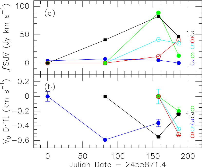
Figure 3: Variabilities of the H₂O 22 GHz maser for each velocity component. The horizontal axis shows the time since the first observing run. (a) Light curve. For the 3, 5, 6, and 8 km s^-1 components, the integrated flux densities are from the spectra toward FIR 6. For the 13 km s^-1 component, the integrated flux densities of the 2012 January/April runs are from the spectra toward FIR 6, corrected for the primary beam attenuation, and that of the 2012 May run is from the spectrum toward FIR 4. (b) Time evolution of centroid velocity with respect to the velocity at the first detection. The velocities of the identified velocity components are labeled.

Figure 3(b) shows variabilities of the centroid velocity. Interestingly, in all cases, the velocity drifted to a lower value (that is, blueshifted) in the first time interval after the appearance. It is unlikely that this phenomenon is owing to an instrumental artifact because the amount and sense of the drifts are all different even in the same time interval. (For example, in the last time interval of Figure 3(b), the 13 km s^-1 component drifted to a higher velocity while the others drifted to lower velocities at various rates.) Those detected three times (the 3 and 13 km s^-1 components) changed the sense of velocity drift. Therefore, the centroid velocity is fluctuating rather than drifting steadily. A typical drift rate is $\sim$0.01 km s^-1 day^-1. The velocity drift is usually interpreted as the acceleration of emission source (e.g., Tofani et al. 1995), but the fluctuations of the velocity seen in the FIR 4/6 masers suggest that the cause of velocity variability is more complicated.

Day-scale variabilities were studied in the 2012 April observing run. Figure 4 shows the change of spectra in two days. A difference of line profile can be seen in the 6 km s^-1 component only. This component became stronger by 10% and redshifted by $\sim$0.09 km s^-1. (For comparison, the intensity variation of the 13 km s^-1 component was smaller than 2%.) The information we can extract from the two spectra is rather limited. Nevertheless, it is clear that the sign of velocity drift in these two days is the opposite of what was seen in a month as describe in the paragraph above, which reinforces the finding that the velocity of emission source fluctuates.

Figure 4: Daily spectra of the H₂O 22 GHz maser line toward FIR 6 in the 2012 April run. (a) Spectra on April 12 (solid line) and 14 (dotted line). (b) Difference between the two days.

3.2 The Methanol Masers

All the three CH₃OH class I maser lines in the tuning ranges of the KVN receivers were detected toward FIR 6. By contrast, other CH₃OH lines were undetected (Table 3), which suggests that the detected lines are amplified emission. Each of the 44 and 95 GHz lines was observed in two observing runs, and there was no detectable time variability.

Figure 5 shows the spectra for each line, and Table 5 lists the line-profile parameters. All the detected CH₃OH emission is confined in a velocity interval around the systemic velocity, within $\sim$2 km s^-1. For the 44 GHz line, the residual spectra of single-component and double-component Gaussian fits show a peak at $\sim$10 km s^-1 higher than the noise level. Therefore, the 44 GHz line seems to show three velocity components. The signal-to-noise ratios of the 95 and 133 GHz lines are too small to tell if there are multiple velocity components.

Figure 5: Spectra of the CH₃OH class I maser lines toward FIR 6. (a) CH₃OH $7_{0}\rightarrow 6_{1}$ $A^{+}$ line. (b) CH₃OH $8_{0}\rightarrow 7_{1}$ $A^{+}$ line. (c) CH₃OH $6_{-1}\rightarrow 5_{0}$ $E$ line. For each line, all the data from the 2011–2012 season were averaged.

Table 5: Parameters of the Methanol Maser Spectra

	$V_{0}$	$S_{p}$	$\Delta V$	$\int SdV$
Line	(km s-1)	(Jy)	(km s-1)	(Jy km s-1)
CH3OH 44 GHz	11.12 $\pm$ 0.08	1.4	2.2 $\pm$ 0.2	03.2 $\pm$ 0.2
CH3OH 44 GHz	10.32 $\pm$ 0.08	1.3	0.8 $\pm$ 0.2	01.1 $\pm$ 0.3
	11.32 $\pm$ 0.08	1.6	0.7 $\pm$ 0.2	01.2 $\pm$ 0.4
	12.21 $\pm$ 0.14	0.9	0.7 $\pm$ 0.3	00.7 $\pm$ 0.3
CH3OH 95 GHz	10.99 $\pm$ 0.13	2.5	1.8 $\pm$ 0.3	04.7 $\pm$ 0.7
CH3OH 133 GHz	10.41 $\pm$ 0.19	7.7	1.7 $\pm$ 0.4	13.7 $\pm$ 2.7

Considering the non-detection of the other CH₃OH lines and the small width of each velocity component of the 44 GHz line, we favor the interpretation that the detected lines are maser emission. However, it is possible that the detected emission can be a mixture of thermal and maser components (e.g., Kalenskii et al. 2010). Additional observations such as interferometric imaging are needed to confirm the nature of this emission.

There is no map of the CH₃OH lines with a sensitivity good enough to constrain the source position, and the YSO(s) responsible for the maser emission can only be deduced from the beam size. Since these lines have different beam sizes (Table 2), it is possible that some emission structure in the beam of a low-frequency line can be outside the beam of a high-frequency line. It is difficult to specify the source of the 44 GHz maser line because there are several embedded objects (FIR 5w/e, 6c/n, and 7) and other YSOs within the beam (Barnes et al. 1989; Skinner et al. 2003; Rodríguez et al. 2003; also see Figure 1(b) of Choi et al. 2012). For the 95 and 133 GHz maser lines, the source is most likely associated with FIR 6c/n because the angular separations of FIR 5 and 7 from FIR 6c ($\sim$25^′′ and 21^′′, respectively) are larger than or comparable to the beam sizes. Note that IRS 22 (Class I YSO; Comerón et al. 1996) is located within the beam.

3.3 The ¹³CS $J$ = 2 $\rightarrow$ 1 Line

The ¹³CS line was observed to measure the systemic velocity of the dense cloud core containing FIR 6. Figure 6 shows the spectrum. The best-fit Gaussian profile gives $V_{0}$ = 10.77 $\pm$ 0.05 km s^-1, peak $T_{\rm mb}$ = 1.95 $\pm$ 0.03 K, $\Delta V$ = 1.66 $\pm$ 0.11 km s^-1, and $\int T_{\rm mb}dV$ = 3.44 $\pm$ 0.19 K km s^-1.

Figure 6: Spectrum of the ¹³CS $J$ = 2 $\rightarrow$ 1 line toward FIR 6. Vertical dotted line: centroid velocity of the best-fit Gaussian profile ($V_{\rm LSR}$ = 10.8 km s^-1).

The systemic velocity of the FIR 6 dense core has been known somewhat poorly because the values in the literature were measured using lines with relatively higher optical depths. Schulz et al. (1991) derived 11.3 km s^-1 using the CS/C³⁴S $J$ = 5 $\rightarrow$ 4 and 7 $\rightarrow$ 6 lines showing widths of 2.5–2.9 km s^-1. Mangum et al. (1999) derived 10.6–10.9 km s^-1 using the H₂CO lines showing widths of 2.3–2.5 km s^-1. For the derivation of systemic velocity, ¹³CS is a better tracer than C³⁴S because of its smaller abundance (Shirley et al. 2003). Indeed, the ¹³CS $J$ = 2 $\rightarrow$ 1 line is much narrower than the lines listed above. Therefore, the systemic velocity of 10.8 km s^-1 derived from the ¹³CS line may be more reliable.

4 DISCUSSION

4.1 FIR 6

The detection of the H₂O and CH₃OH masers suggests that the NGC 2024 FIR 6 region is actively forming stars, which produces shocks in the warm and dense molecular gas around the YSOs. The two maser species show the well-known contrasting characteristics (Menten 1991; Elitzur 1992). The H₂O maser emission can be seen in a relatively wide range of velocities while the CH₃OH maser emission is confined in a narrow range around the systemic velocity of the cloud. The H₂O maser also displays strong variabilities in both amplitude and velocity, while the CH₃OH masers show no detectable variability.

The most likely exciting source of the H₂O maser reported in this paper is FIR 6n. The maser probably comes from the base of the bipolar outflow driven by FIR 6n (Richer 1990; Choi et al. 2012). During the observation period covered in this study, all the H₂O emission was blueshifted with respect to the systemic velocity of the FIR 6 core, and the blueshifted outflow may have been responsible for the observed H₂O maser emission. However, the emission was nearly at the systemic velocity in 1995/1996 (Choi et al. 2012), and both blueshifted and redshifted velocity components were detected in 1999 (Furuya et al. 2003).

The variability of the FIR 6 H₂O maser is typical of low-mass YSO. The typical life time of each velocity component is $\sim$8 months. This timescale is generally consistent with the values reported in surveys toward low-mass YSOs, which range from $\sim$2 weeks to $\sim$8 months (Wilking et al. 1994; Furuya et al. 2003). The velocity drift rate of the FIR 6 H₂O maser is similar to that reported by Tofani et al. (1995). Note that the time interval between observing runs in this study is not short enough to trace variabilities at timescales shorter than about a month.

The interpretation of the CH₃OH class I masers is unclear. Soon after the discovery of the CH₃OH masers, it was found that class I masers trace outflows driven by high-mass YSOs and are located away from the responsible YSOs up to $\sim$2 pc (Plambeck & Menten 1990; Kurtz et al. 2004). Recently, however, it was found that some class I masers may be associated with shocks driven into molecular clouds by expanding H II regions (Voronkov et al. 2010; Chen et al. 2011) and that several low-mass star forming regions emit class I masers (Kalenskii et al. 2010). If the FIR 6 CH₃OH masers trace an expanding H II region, the FIR 6c hypercompact H II region (candidate) may be responsible. If they trace an outflow, the FIR 6n bipolar outflow may be responsible for the masers. If the maser emission comes from the FIR 6n outflow, it would be one of the rare examples of CH₃OH maser associated with low-mass YSOs. This issue can be settled by future observations using interferometers.

4.2 FIR 4

The detection of the H₂O maser toward FIR 4 illustrates the importance of mapping in single-dish observations of H₂O masers. While this paper gives the first confirmation of the H₂O maser associated with FIR 4, it is not necessarily the first detection. For example, Furuya et al. (2003) reported single-dish observations toward FIR 5/6 (see their Figure 13(a)). Since FIR 4–6 are within their beam, it is likely that the detected emission in their spectra were mostly from FIR 4/6. (Note that interferometric observations never showed an H₂O maser associated with FIR 5.) Our recent survey also confirmed that multiple H₂O maser sources in a single-dish beam is a common occurrence in cluster-forming regions such as the Orion cloud (M. Kang et al. 2012, in preparation). The exciting source of H₂O maser emission in a given detection is not necessarily the previously known source, the youngest YSO in the beam, or the most powerful outflow source in the beam. This problem can affect some statistical quantities derived from single-dish surveys, such as detection rates, and can be worse in massive star forming regions far away from the Sun.

The H₂O maser suggests that there are shocks produced by the star formation activities of FIR 4. The nature of FIR 4, however, has been controversial. Early studies indicated the existence of dense gas in the NGC 2024 region (Evans et al. 1987). Mezger et al. (1988, 1992) suggested that the FIR 1–7 cores are isothermal protostars without luminous stellar objects, based on their dust continuum observations. Studies with molecular (thermal) lines suggested that they contain more evolved YSOs (Schulz et al. 1991; Mangum et al. 1999). The discovery of a near-IR reflection nebula and a CO outflow revealed that FIR 4 contains a low-mass YSO driving a bipolar outflow (Moore & Chandler 1989; Moore & Yamashita 1995; Chandler & Carlstrom 1996). A very different view was proposed by Minier et al. (2003). They detected the CH₃OH class II maser line at 6.7 GHz in emission and argued that FIR 4 contains an intermediate or high-mass YSO. Future investigations are needed to tell whether low-mass protostars can produce CH₃OH class II maser emission or FIR 4 is a site of high-mass star formation. The detection of the H₂O maser does not necessarily favor one or the other possibility.

It is interesting to note that there are position offsets of $\sim$2^′′ among the 3 mm continuum, CH₃OH class II maser, and hard X-ray positions (Chandler & Carlstrom 1996; Minier et al. 2003; Skinner et al. 2003). Future determinations of the accurate position of the H₂O maser source will be helpful in understanding the nature of FIR 4.

5 SUMMARY

The NGC 2024 FIR 6 region was observed using the KVN in the H₂O 22 GHz maser line, the CH₃OH 44, 95, and 133 GHz class I maser lines, other CH₃OH lines in the tuning ranges, and the ¹³CS $J$ = 2 $\rightarrow$ 1 line in the single-dish telescope mode. In addition, the FIR 4 region was observed in the H₂O line. The main results are summarized as follows.

1. Several velocity components were identified in the H₂O spectra. The H₂O maps revealed that most of them seem to be associated with FIR 6n while one is associated with FIR 4. None is associated with FIR 5.

2. Month-scale variabilities of the H₂O maser were seen clearly. A typical life time of each velocity component is $\sim$8 months. The centroid velocity fluctuates with a drift rate of $\sim$0.01 km s^-1 day^-1.

3. The CH₃OH class I maser lines were detected toward FIR 6. They were interpreted as maser emission. The maser emission is confined within $\sim$2 km s^-1 around the systemic velocity of the cloud. It is not clear whether the exciting source is FIR 6c or 6n. The CH₃OH masers did not show a detectable time-variability. High-resolution imaging is needed to understand whether the CH₃OH maser emitting region is shocked by an outflow or an expanding H II region.

4. The other CH₃OH lines, thermal or class II maser, were not detected.

5. The ¹³CS spectrum showed that the systemic velocity of the FIR 6 dense core is $\sim$10.8 km s^-1.

References

- (1) Alves, F. O., Girart, J. M., Lai, S.-P., Rao, R., & Zhang, Q. 2011, ApJ, 726, 63
- (2) Anthony-Twarog, B. J. 1982, AJ, 87, 1213
- (3) Barnes, P. J., Crutcher, R. M., Bieging, J. H., Storey, J. W. V., & Willner, S. P. 1989, ApJ, 342, 883
- (4) Baudry, A., Lucas, R., & Guilloteau, S. 1995, A&A, 293, 594
- (5) Chandler, C. J., & Carlstrom, J. E. 1996, ApJ, 466, 338
- (6) Chen, X., Ellingsen, S. P., Shen, Z.-Q., Titmarsh, A., & Gan, C.-G. 2011, ApJS, 196, 9
- (7) Choi, M., Lee, J.-E., & Kang, M. 2012, ApJ, 747, 112
- (8) Comerón, F., Rieke, G. H., & Rieke, M. J. 1996, ApJ, 473, 294
- (9) Cragg, D. M., Johns, K. P., Godfrey, P. D., & Brown, R. D. 1992, MNRAS, 259, 203
- (10) Crutcher, R. M., Henkel, C., Wilson, T. L., Johnston, K. J., & Bieging, J. H. 1986, ApJ, 307, 302
- (11) Elitzur, M. 1992, ARA&A, 30, 75
- (12) Evans, N. J., II, Davis, J. H., Mundy, L. G., & Vanden Bout, P. 1987, ApJ, 312, 344
- (13) Furuya, R. S., Kitamura, Y., Wootten, A., Claussen, M. J., & Kawabe, R. 2003, ApJS, 144, 71
- (14) Genzel, R., & Downes, D. 1977, A&AS, 30, 145
- (15) Johnston, K. J., Sloanaker, R. M., & Bologna, J. M. 1973, ApJ, 182, 67
- (16) Kalenskii, S. V., Johansson, L. E. B., Bergman, P., et al. 2010, MNRAS, 405, 613
- (17) Kurtz, S., Hofner, P., & Álvarez, C. V. 2004, ApJS, 155, 149
- (18) Lada, E. A., Bally, J., & Stark, A. A. 1991, ApJ, 368, 432
- (19) Lai, S.-P., Crutcher, R. M., Girart, J. M., & Rao, R. 2002, ApJ, 566, 925
- (20) Lee, S.-S., Byun, D.-Y., Oh, C. S., et al. 2011, PASP, 123, 1398
- (21) Mangum, J. G., Wootten, A., & Barsony, M. 1999, ApJ, 526, 845
- (22) Menten, K. 1991, Atoms, Ions and Molecules: New Results in Spectral Line Astrophysics (ASP Conf. Ser. 16), ed. A. D. Haschick & P. T. P. Ho (San Francisco, CA: ASP), 119
- (23) Mezger, P. G., Chini, R., Kreysa, E., Wink, J. E., & Salter, C. J. 1988, A&A, 191, 44
- (24) Mezger, P. G., Sievers, A. W., Haslam, C. G. T., et al. 1992, A&A, 256, 631
- (25) Minier, V., Ellingsen, S. P., Norris, R. P., & Booth, R. S. 2003, A&A, 403, 1095
- (26) Moore, T. J. T., & Chandler, C. J. 1989, MNRAS, 241, 19P
- (27) Moore, T. J. T., & Yamashita, T. 1995, ApJ, 440, 722
- (28) Müller, H. S. P., Menten, K. M., & Mäder, H. 2004, A&A, 428, 1019
- (29) Plambeck, R. L., & Menten, K. M. 1990, ApJ, 364, 555
- (30) Richer, J. S. 1990, MNRAS, 245, 24P
- (31) Rodríguez, L. F., Gómez, Y., & Reipurth, B. 2003, ApJ, 598, 1100
- (32) Schulz, A., Güsten, R., Zylka, R., & Serabyn, E. 1991, A&A, 246, 570
- (33) Shirley, Y. L., Evans, N. J., II, Young, K. E., Knez, C., & Jaffe, D. T. 2003, ApJS, 149, 375
- (34) Skinner, S., Gagné, M., & Belzer, E. 2003, ApJ, 598, 375
- (35) Tofani, G., Felli, M., Taylor, G. B., & Hunter, T. R. 1995, A&AS, 112, 299
- (36) Visser, A. E., Richer, J. S., Chandler, C. J., & Padman, R. 1998, MNRAS, 301, 585
- (37) Voronkov, M. A., Caswell, J. L., Ellingsen, S. P., & Sobolev, A. M. 2010, MNRAS, 405, 2471
- (38) Wiesemeyer, H., Guesten, R., Wink, J. E., & Yorke, H. W. 1997, A&A, 320, 287
- (39) Wilking, B. A., Claussen, M. J., Benson, P. J., et al. 1994, ApJ, 431, L119