An Improved dqds algorithm

Abstract

In this paper we present an improved dqds algorithm for computing all the singular values of a bidiagonal matrix to high relative accuracy. There are two key contributions: a novel deflation strategy that improves the convergence for badly scaled matrices, and some modifications to certain shift strategies that accelerate the convergence for most bidiagonal matrices. These techniques together ensure linear worst case complexity of the improved algorithm (denoted by V5). Our extensive numerical experiments indicate that V5 is typically 1.2x–4x faster than DLASQ (the LAPACK-3.4.0 implementation of dqds) without any degradation in accuracy. On matrices for which DLASQ shows very slow convergence, V5 can be 3x–10x faster. At the end of this paper, a hybrid algorithm (HDLASQ) is developed by combining our improvements with the aggressive early deflation strategy (AggDef2 in [SIAM J. Matrix Anal. Appl., 33(2012), 22-51]). Numerical results show that HDLASQ is the fastest among these different versions.

1 Introduction

The dqds (differential quotient difference with shifts) algorithm of [5] computes the singular values of bidiagonal matrices to high relative accuracy. A detailed account of its efficient implementation, which is essentially the LAPACK code, can be found in [16]. One critical technique responsible for its success is the rather complex shift strategy. An aggressive early deflation (AED) strategy is suggested in [12] to further enhance performance for large matrices.

Our work is motivated by the recent discovery of significant slowdown of the LAPACK routine DLASQ on certain matrices which have diagonal and off-diagonal entries that are of varying magnitude and are disordered (far from monotone decreasing). The improvements of our algorithm are

1. the ability to deflate converged singular values that are far from the bottom of the matrix;

2. an improved bound on the current smallest singular value;

3. some modifications to certain shift strategies;

4. a guarantee that the convergence is never slower than that for the bisection algorithm.

Our improved implementation (denoted by V5) is 1.2x-4x faster than DLASQ in general and up to 10x faster for matrices for which the dqds algorithm converges slowly. It should be mentioned that the dqds algorithm has found other uses than computation of the singular values and the ideas in this paper may be of value in those situations as well [6].

V5 is never slower than the bisection algorithm in convergence, which establishes its linear complexity in the worst case and ensures a more robust implementation of the dqds algorithm. There is a similar result for the QR algorithm with Wilkinson shift for the symmetric tridiagonal eigenproblems [14].

V5 and AED are complementary: AED may help for matrices which are easy for dqds, whereas V5 improves the convergence for the disordered matrices. By combining V5 with AED, a more efficient algorithm is obtained in section 6. This hybrid algorithm would be denoted by HDLASQ and is shown to be faster than DLASQ, V5 and AggDef2 (proposed in [12]) for both the easy and difficult matrices.

This paper is organized as follows. Sections 2 and 3 introduce the dqds algorithm and its LAPACK implementation DLASQ, respectively. Section 4 discusses the five important improvements over DLASQ. Section 5 proves the linear worst case complexity of V5. Section 6 compares V5 with DLASQ and AggDef2, and introduces the hybrid algorithm HDLASQ. Numerous experiments on synthetic and practical matrices are also reported in section 6. Section 7 presents the conclusions.

2 Essential information on dqds

In this section we gather essential properties of the dqds algorithm. The reader is expected to have some acquaintance with this algorithm. For an introduction to the topic we recommend [13] and for historical details [5]. By convention our bidiagonal matrices are all upper bidiagonal. Our notation is as follows

$$B=\begin{bmatrix}a_{1}&b_{1}&&&&\\ &a_{2}&b_{2}&&&\\ &&\cdotp&\cdotp&&\\ &&&\cdotp&\cdotp&\\ &&&&a_{n-1}&b_{n-1}\\ &&&&&a_{n}\end{bmatrix},$$ (1)

and all the elements of $B$ are positive.

In addition to the dqds algorithm we refer to a simpler procedure oqd (orthogonal qd) that transforms $B$ into $\hat{B}$ so that

$$BB^{T}=\hat{B}^{T}\hat{B},$$

see [5].

Algorithm 1. [oqd] $\tilde{a}_{1}=a_{1}$ for $k=1,\cdots,n-1$ $\hat{a}_{k}:=\sqrt{\tilde{a}_{k}^{2}+b_{k}^{2}}$ $\hat{b}_{k}:=b_{k}*(a_{k+1}/\hat{a}_{k})$ $\tilde{a}_{k+1}:=\tilde{a}_{k}*(a_{k+1}/\hat{a}_{k})$ end for $\hat{a}_{n}:=\tilde{a}_{n}$   Algorithm 2. [dqds] $d_{1}=q_{1}-s$, for $k=1,\cdots,n-1$ $\hat{q}_{k}:=d_{k}+e_{k}$ $\hat{e}_{k}:=e_{k}*(q_{k+1}/\hat{q}_{k})$ $d_{k+1}=d_{k}*(q_{k+1}/\hat{q}_{k})-s$ end for $\hat{q}_{n}:=d_{n}$

The dqd algorithm can be obtained by squaring the variables in the oqd algorithm,

$$q_{k}=a_{k}^{2},\quad e_{k}=b_{k}^{2},\quad k=1,2,\cdots,n,\quad b_{n}=0.$$ (2)

The dqds algorithm is obtained by incorporating a shift in the dqd algorithm. The shift will be denoted by s.

The point of introducing oqd is to exhibit the relation of the $\{q,e\}$ variables to the $\{a,b\}$ variables of $B$. However an alternative connection is to define

$$L=\begin{bmatrix}1&&&&&\\ e_{1}&1&&&&\\ &e_{2}&.&&&\\ &&.&.&&\\ &&&.&1&\\ &&&&e_{n-1}&1\end{bmatrix},\quad U=\begin{bmatrix}q_{1}&1&&&&\\ &q_{2}&1&&&\\ &&.&.&&\\ &&&.&.&\\ &&&&.&1\\ &&&&&q_{n}\end{bmatrix}.$$

With some algebraic manipulations, one can show that the dqds algorithm implements the transform

$$\hat{L}\hat{U}=UL-sI.$$ (3)

One step of the dqds transform is to compute $\hat{L}$ and $\hat{U}$ from $L$ and $U$.

An essential ingredient in the success of dqds is that it never explicitly forms any products $UL$ or $LU$ but works entirely with the factors. Furthermore, $LU$ and $B^{T}B$ are connected by a diagonal similarity transformation [13],

$$LU=\Delta B^{T}B\Delta^{-1},$$ (4)

where

$$\Delta=\mathop{\operator@font diag}\nolimits(1,\pi_{1},\pi_{1}\pi_{2},\ldots,\pi_{1}\cdots\pi_{n-1}),\quad\pi_{i}=a_{i}b_{i}.$$

Therefore $LU$ and $B^{T}B$ have the same eigenvalues, and $\sigma(B)=\sqrt{\lambda(LU)}$.

Recall that one step of the LR algorithm [15] transforms the matrix $A$ into matrix $\hat{A}$ by

$$\begin{split}A-sI&=\tilde{L}\tilde{U},\\ \hat{A}&=\tilde{U}\tilde{L}+sI,\end{split}$$

where $\tilde{L}$ is a lower triangular matrix and $\tilde{U}$ is an upper triangular matrix. Note that $\hat{A}=\tilde{L}^{-1}A\tilde{L}$. We say that the shift is restored. In contrast to the LR algorithm, the dqds transform is a non-restoring similarity transformation on $UL$,

$$\hat{U}\hat{L}=\hat{L}^{-1}(\hat{L}\hat{U})\hat{L}=\hat{L}^{-1}(UL-sI)\hat{L}.$$ (5)

Notice that $\hat{U}\hat{L}$ is not similar to $UL$ and the shift $s$ is not restored. After each dqds transform, all eigenvalues are reduced by $s$. Because of the non-restoring feature, the dqds algorithm must keep track of the accumulated shifts, $S=\sum_{i=1}^{k}s_{i}$.

The dqds algorithm is the repeated applications of the dqds transform with a sequence of well chosen shifts. This algorithm checks, before each transform, whether $e_{n-2}$ or $e_{n-1}$ is negligible. If so then one or two eigenvalues have been computed accurately and the computation resumes on a smaller array. This process is called deflation. A well known feature of the QR-type and LR-type algorithms is that the larger entries migrate gradually to the top of the matrix and the smaller ones precipitate to the bottom. The smaller they are the quicker they fall. That is why the classical deflation strategies detect the bottom $2\times 2$ submatrix.

Detecting small entries above the bottom is also very important. Setting a negligible $e_{k}$ to zero where $k<n-2$ is usually called splitting [16] instead of deflation. In this case, a big problem breaks into two independent smaller problems. It is vital to check for splitting since, if $e_{k}=0$, the two subarrays should be treated independently; whereas a tiny $e_{k}\neq 0$ could signficantly slow down convergence if left untreated. The criteria for negligibility have received careful attention and the tests can be complicated. A novel deflation strategy is proposed in section 4.1 for the case when an intermediate variable ($e_{k}$ or $d_{k}$ for $k<n-2$) is negligible.

In the 1960s Kahan proved that a bidiagonal matrix defines all its singular values to high relative accuracy, see [3]. In the context of dqds this precious feature will be preserved if all the $\{q,e\}$ variables remain positive [5]. Thus the shift $s$ must obey

$$s<\lambda_{\min}(BB^{T}).$$ (6)

This constraint means that the singular values must be found in monotone increasing order. This is in contrast to the QR algorithm with shifts but the QR algorithm does not claim to compute the eigenvalues to high relative accuracy except when the shifts are zero.

The $\{q,e\}$ variables require so little storage that it is sensible to compute $\{\hat{q},\hat{e}\}$ in a separate location from $\{q,e\}$, and then decide whether to accept or reject the transform. If any new variables are negative the algorithm rejects the transform and chooses a smaller shift. This is called a failure. The ability to reject a transform permits an aggressive shift strategy.

2.1 Some theoretical results

In the following sections we use the $B$ notation to describe the dqds algorithm.

Theorem 1 (Theorem 2 in [5]).

Apply the dqd transform (not dqds) to a positive bidiagonal matrix $B$ and $d_{1},\cdots,d_{n}$ are the intermediate values. Then

1. $\sigma_{\min}^{2}(\hat{B})\leq\min_{k}\{d_{k}\}$,

2. $[(BB^{T})^{-1}]_{k,k}=d_{k}^{-1}$,

3. $(\sum_{k=1}^{n}d_{k}^{-1})^{-1}\leq\sigma_{\min}^{2}$.

From item 1 $d_{\min}=\min_{k}\{d_{k}\}\geq\sigma_{\min}^{2}(\hat{B})$. Asymptotically $d_{\min}$ is a very good estimate of $\sigma_{\min}^{2}(\hat{B})$, and therefore DLASQ records $d_{\min}$ as a guide to choosing a shift. But at the early stage $d_{\min}$ may be too big. There is more on this topic later.

Corollary 2.

With the notation in Theorem 1, we have

$$\frac{1}{n}d_{\min}\leq\sigma_{\min}^{2}(\hat{B})\leq d_{\min}\leq n\sigma_{\min}^{2}(\hat{B}).$$ (7)

Corollary 2 implies that $d_{\min}$ becomes negligible when the matrix becomes nearly singular. It is the basis of our deflation strategy in section 4.1. There are similar results for the dqds algorithm.

Theorem 3 (Theorem 3 in [5]).

If the dqds with shift $s\geq 0$ transforms positive bidiagonal matrix $B$ into positive $\hat{B}$ with intermediate quantities $d_{1},\cdots,d_{n}$ then

1. $\sigma_{\min}^{2}(\hat{B})\leq\min_{k}\{d_{k}\}$,

2. $[(BB^{T})^{-1}]_{k,k}<d_{k}^{-1}$,

3. $(\sum_{k=1}^{n}d_{k}^{-1})^{-1}<\sigma_{\min}^{2}(\hat{B})$.

Corollary 4.

$$\begin{split}\frac{1}{n}d_{\min}<&\sigma_{\min}^{2}(\hat{B})\leq d_{\min}<n\sigma_{\min}^{2}(\hat{B}).\end{split}$$ (8)

These two corollaries have very important practical implications.

• A good shift should always be in $[\frac{d_{\min}}{n},d_{\min}]$.

• A very small $\sigma_{n}^{2}(\hat{B})$ automatically implies a very small $d_{\min}$. If $d_{\min}$ is negligible then it is possible to deflate the matrix even if $d_{\min}=d_{k}$, $k\ll n$, see section 4.1.

3 Features of the current LAPACK implementation

The algorithm presented in [16] was designed for speed on all the test matrices available before 2000. It was on average 5x faster than the Demmel-Kahan QR code for computing singular values [16]. The drive for efficiency produced a more complex shift strategy than that used in the previous LR/QR codes for the tridiagonal eigenvalue problems. As an example, by unrolling the last 3 minor steps, the code keeps values $d_{n-2},d_{n-1}$ and $d_{n}$ available so that, in the asymptotic regime, there is enough information to make a good approximation to the new $\sigma_{\min}$ even after one or two eigenvalues are deflated. For example, $d_{n-2}$ might be $d_{\min}$ for the deflated array.

The code keeps the information for both $\{q,e\}$ and $\{\hat{q},\hat{e}\}$. If any entry in $\hat{q}$ or $\hat{e}$ is negative the transform is rejected and the step is considered a failure and aborted. Consequently an aggressive shift strategy may be employed. But the number of failures should be kept small. Too many failures will surely degrade the performance. To enhance data locality, the variables are held in one linear array

$$Z=\{q_{1},\hat{q}_{1},e_{1},\hat{e}_{1},q_{2},\hat{q}_{2},e_{2},\hat{e}_{2},\cdots,q_{n},\hat{q}_{n}\}.$$

The dqds maps $\{q,e\}$ to $\{\hat{q},\hat{e}\}$ and vice versa to avoid data movement. This is called ping-pong implementation in [16].

The implementation of dqds in the LAPACK, as of 2000, is based on the following perception.

“An explicit conditional statement (if-then-else) in an inner loop impedes efficient implementation on a pipelined arithmetic unit.”

Consequently the division in the dqds loop, $t=q_{k+1}/\hat{q}_{k}$, is not protected from incurring an exception (divide by zero or overflow). However, the powerful feature of arithmetic units conforming to IEEE floating point standard 754 is that computation is not held up by an exception. At the end of the loop the code tests whether an $\infty$ or a NaN (not a number) occurred and acts appropriately.

The LAPACK implementation also assumes that a good compiler will implement the intrinsic FORTRAN functions such as MIN(A,B) or MAX(A,B) efficiently. Hence the valuable variable $d_{\min}$ is computed via $d_{\min}$= MIN($d_{k},d_{\min}$) in the inner loop.

This implementation also gives up the knowledge of the index at which $d_{\min}$ receives its final value since this would require an explicit conditional,

1. if $d_{k}<d_{\min}$ then

2. dmink=$k$; $d_{\min}=d_{k}$;

3. end if

where the position of $d_{\min}$ is denoted by $dmink$. However, our efficiency enhancements require knowledge of the index of $d_{\min}$. This explicit conditional statement need not impede performance provided that it is placed, not in its natural position, but immediately after the division. This is because division is so slow relative to other operations, such as comparison, that the conditional statement can be completed before the preceding division finishes. Technically this requires us to update $d_{\min}$ one minor step late but that is easily dealt with. Algorithm 3 is the inner loop of a new implementation.

Algorithm 3. [inner loop of the dqds algorithm] for $k=1$ to $n-1$ $\hat{q}_{k}=d_{k}+e_{k}$; $t=q_{k+1}/\hat{q}_{k}$; if $d_{k}<0$ then exit (early failure); else if $d_{k}<d_{\min}$ then dmink=$k$; $d_{\min}=d_{k}$; end if end if $\hat{e}_{k}=e_{k}\cdotp t$; $d_{k+1}=d_{k}\cdotp t-s$; end for if $d_{n}<0$ then continue (late failure); else if $d_{n}<d_{\min}$ then dmink=$n$; $d_{\min}=d_{n}$; end if

If $d_{k}<0$ ($k<n$) and shift $s>0$, then by Algorithm 2 the dqds algorithm may fail in three possible ways: $\hat{q}_{j}$ ($k<j<n$) is negative or zero, or $\hat{q}_{n}<0$. The case ($d_{k}<0,k<n$) is called an early failure. A late failure occurs when the arrays $\{\hat{q}_{k},\hat{e}_{k}\}$ are all positive except for the last $\hat{q}_{n}=d_{n}<0$. In the case of a late failure, a smaller shift can be chosen as $s+d_{n}$, which is guaranteed to succeed. This property was discovered by H. Rutishauser. See [16] for details.

4 Improvements

In this section, we summarize the improvements of our implementation over DLASQ, which can be divided into two types: deflation strategies and shift strategies.

4.1 Setting negligible $d_{\min}$ to zero

Recall that the dqds algorithm is non-restoring. The algorithm tries at every step to make the current matrix singular. The positive $\{q,e\}$ array defines both a positive bidiagonal matrix $B$ and the matrices $L$, $U$, see [13]. It can happen that a leading principal submatrix of $B$ becomes almost singular long before any negligible entries appear at the bottom of the matrix. This situation is not easily detected by a simple inspection of the entries $\{q_{k},e_{k}\}$, or say $\{a_{k},b_{k}\}$.

To explain, it is best to go back to the oqd transform from $B^{T}$ to $\hat{B}$, and consider the process after ($k-1$) minor steps shown in the following equation,

$$B^{(k)}=Q_{k}B^{T}=\begin{bmatrix}\hat{a}_{1}&\hat{b}_{1}&&&&&&&&\\ 0&\hat{a}_{2}&\hat{b}_{2}&&&&&&&\\ &0&\cdotp&\cdotp&&&&&&\\ &&0&\hat{a}_{k-1}&\hat{b}_{k-1}&&&&&\\ &&&0&\tilde{a}_{k}&0&&&&\\ &&&&b_{k}&a_{k+1}&0&&&\\ &&&&&b_{k+1}&a_{k+2}&&\\ &&&&&&\cdotp&\cdotp&0&\\ &&&&&&&b_{n-1}&a_{n}\end{bmatrix}.$$ (9)

The striking feature is that row $k$ is a singleton, its entry is $\tilde{a}_{k}$ and $\tilde{a}_{k}^{2}=d_{k}$. Rows ($1:k$) are upper bidiagonal, rows ($k:n$) are lower bidiagonal. Such matrices are often described as twisted. Corollary 2 says $\tilde{a}_{k}$ would be small when $\hat{B}$ is nearly singular. How small must $\tilde{a}_{k}$ be to declare it negligible? Define new matrices $\tilde{B}$ and $E$, using equation (9), by

$$B^{(k)}=Q_{k}B^{T}=\tilde{B}+E,$$

where row $k$ of $\tilde{B}$ is null and $E=\text{diag}(0,\cdots,0,\tilde{a}_{k},0,\cdots,0)$. Observe that $E\tilde{B}=E^{T}\tilde{B}=0$. Hence,

$$\begin{split}B^{(k)T}B^{(k)}&=(\tilde{B}+E)^{T}(\tilde{B}+E)\\ &=\tilde{B}^{T}\tilde{B}+\tilde{B}^{T}E+E^{T}\tilde{B}+E^{T}E\\ &=\tilde{B}^{T}\tilde{B}+E^{T}E.\end{split}$$ (10)

By Weyl’s monotonicity theorem [8, Thm. 3.3.16]), for $i=1:n$,

$$|\sigma_{i}^{2}-\tilde{\sigma}_{i}^{2}|\leq\|E^{2}\|=d_{k}.$$ (11)

Here $\{\tilde{\sigma}_{i}^{2}\}$ are the ordered singular values of $\tilde{B}$. The non-restoring character of the dqds algorithm entails that the desired eigenvalues are $\{\sigma_{i}^{2}+S\}$ where $S$ is the accumulated sum of shifts so far. Consequently, $d_{k}$ ($\tilde{a}_{k}^{2}$) may be set to zero, when

$$d_{k}\leq\epsilon S\leq\epsilon(S+\sigma_{i}^{2}).$$

How to deflate by exploiting such an event? Examination of the inner loop of oqd, Algorithm 2, shows that with $\tilde{a}_{k}=0$, the algorithm simply moves the remaining variables into new positions

$$\hat{a}_{j}=b_{j},\text{ }\hat{b}_{j}=a_{j+1},\text{ }j=k,\ldots,n-1,\text{ and }\hat{a}_{n}=\tilde{a}_{k}=0.$$

The bidiagonal $\hat{B}$ reveals its singularity ($\hat{a}_{n}=0$) but deflation requires that $\hat{b}_{n-1}$ also vanishes. More work needs to be done since $\hat{b}_{n-1}=a_{n}$ may not be negligible. There are two options.

Option A. Apply the oqd transform to $\hat{B}$ to obtain $\bar{B}$ and note that $\bar{b}_{n-1}=\hat{b}_{n-1}(\hat{a}_{n}/\bar{a}_{n-1})=0$, $\bar{a}_{n}=\tilde{a}_{n-1}(\hat{a}_{n}/\bar{a}_{n-1})=0$. The new singular value is $S+\hat{a}_{n}=S$ and $n\leftarrow n-1$. In practice the dqd transform is used, not oqd.

Option B. The procedure invoked in the aggressive early deflation algorithm, see [12], is useful here. In our implementation we use this option since we found it usually saves some floating point operations over Option A. We describe it briefly.

Apply a carefully chosen sequence of plane rotations on the right of $\hat{B}$ to chase the entry $\hat{b}_{n-1}$ up in the last column of $\hat{B}$. The sequence of ‘planes’ is $(n-1,n)$, $(n-2,n),(n-3,n),\cdots,(1,n)$. The single nonzero entry $\psi$ in the last column is called the bulge. Its initial value is $\hat{b}_{n-1}$ and it shrinks as it rises up. The expectation is that the bulge will become negligible quickly, in fewer than 10 rotations.

Let ${\bf e}_{i}$, $i=1,\ldots,n$, be the $i$-th column of an $n\times n$ identity matrix (to distinguish from $e_{i}$). When the bulge is in position $(k,n),k\leq n-1$, the matrix can be written as $\overset{o}{B}+E$ where $E=\psi{\bf e}_{k}{\bf e}_{n}^{T}$ and $\overset{o}{B}$’s last row and column are null. Then $(\overset{o}{B}+E)(\overset{o}{B}+E)^{T}=\overset{o}{B}\overset{o}{B^{T}}+\psi^{2}{\bf e}_{k}{\bf e}_{k}^{T}$. It turns out that the criterion for neglecting the bulge $\psi$ is the same as the criterion for neglecting $d_{k}$, namely

$$\psi^{2}\leq\epsilon S,$$

and $\psi^{2}$ is expressible in terms of $\{q_{i},e_{i}\}$.

To be more specific, let $\psi=\sqrt{x}$. The bulge moves upward by one position by applying a Givens transformation from the right [12]:

$$\begin{bmatrix}*&*&&&\\ &*&*&&\\ &&*&\sqrt{e_{k}}&\\ &&&\sqrt{q_{k+1}}&\sqrt{x}\\ &&&&0\end{bmatrix}\underrightarrow{G_{k}}\begin{bmatrix}*&*&&&\\ &*&*&&\\ &&&\sqrt{\bar{e}_{k}}&\sqrt{\bar{x}}\\ &&&\sqrt{\bar{q}_{k+1}}&0\\ &&&&0\end{bmatrix},$$

where $G_{k}$ is an orthogonal matrix of the form $\begin{bmatrix}c&s\\ s&-c\end{bmatrix}$ to keep the entries of $B$ positive. The values $\bar{q}_{k+1}$, $\bar{e}_{k}$ and $\bar{x}$ can be computed as

$$\bar{q}_{k+1}=q_{k+1}+x,\quad\bar{e}_{k}=\frac{q_{k+1}e_{k}}{q_{k+1}+x},\quad\bar{x}=\frac{xe_{k}}{q_{k+1}+x}.$$

The whole algorithm is described as follows, where $\bar{q},\bar{e}$ and $\bar{x}$ are also denoted by $q,e$ and $x$ respectively.

Algorithm 4. [Option B] $x=e_{n-1}$; for $k=n$-$1,n$-$2,\cdots,2$ $t_{1}=q_{k}$; $q_{k}=q_{k}+x$; $t_{2}=1/q_{k}$; $x=x\cdotp e_{k-1}\cdotp t_{2}$; $e_{k-1}=e_{k-1}\cdotp t_{1}\cdotp t_{2}$; if $x$ is negligible, break; end for if $k=1$,  $q_{1}=q_{1}+x$;

Remark 4.5.

The deflation strategy, setting negligible $d_{\min}$ to zero, is the most important improvement over DLASQ and is ‘tailor-made’ for the disordered matrices for which the dqds algorithm shows slow convergence. This deflation will be called d-deflation strategy in later sections.

4.2 Improved criterion for late deflation

A crude, but adequate, criterion for setting $b_{n-1}$ (in $B$) to zero, is

$$|b_{n-1}|<c\epsilon(\sqrt{S}+\sigma_{{\min}}(B)),$$

where $\epsilon$ is the machine precision and $c$ is a modest constant, for example $c=10$ in DLASQ and in our implementation. In the context of a $\{q,e\}$ array this same criterion becomes approximately

$$e_{n-1}<(c\epsilon)^{2}S.$$ (12)

Note that $q_{n}=d_{n}$ usually becomes very small, see Lemma 5.3 [1] or Lemma .12 in the Appendix. Instead of only testing $e_{n-1}$, a more refined criterion arises from considering the trailing $2\times 2$ submatrix of $BB^{T}$,

$$\begin{bmatrix}a_{n-1}^{2}+b_{n-1}^{2}&b_{n-1}a_{n}\\ b_{n-1}a_{n}&a_{n}^{2}\end{bmatrix}.$$

By Weyl’s theorem no eigenvalue of $BB^{T}$ changes by no more than $b_{n-1}a_{n}$ if the $2\times 2$ matrix $\begin{bmatrix}0&b_{n-1}a_{n}\\ b_{n-1}a_{n}&0\end{bmatrix}$ is subtracted from the trailing $2\times 2$ submatrix shown above. However the $(n-1,n-1)$ entry of $BB^{T}$ still involves $b_{n-1}^{2}$. No eigenvalue of $BB^{T}$ can change by more than $b_{n-1}^{2}$ if it is neglected. We can set it to zero when it is negligible compared to either $S+\lambda_{\min}(BB^{T})$ or $a_{n-1}^{2}$. Consequently the crude criterion (12) may be replaced by the following pair of tests:

$$b_{n-1}^{2}<c\epsilon\max(S,a_{n-1}^{2})\text{ and }b_{n-1}a_{n}<c\epsilon(S+\lambda_{\min}(BB^{T}).$$

In the context of $\{q,e\}$ array, we use

$$e_{n-1}<c\epsilon\max(S,q_{n-1})\text{ and }e_{n-1}q_{n}<(c\epsilon S)^{2}.$$ (13)

The same arguments can give us a more refined test for splitting $B$ whenever $e_{k}$ and $e_{k}q_{k+1}$ are negligible.

4.3 Updating the upper bound

In his original papers on the qd algorithm, Rutishauser proposed updating the upper and lower bounds, sup and inf, on $\sigma_{\min}^{2}(B)$ at all times. The original paper [5] on the dqds algorithm followed the recommendation but the implementation DLASQ [16] omitted to update sup when a transform failed.

A transform $\{q,e\}$ into $\{\hat{q},\hat{e}\}$ fails if any entry in $\hat{q}$ or $\hat{e}$ is nonpositive (but $\hat{q}_{n}=0$ is permitted). In this case the connection to a bidiagonal $\hat{B}$ is lost. It can only happen if the shift $s$ exceeds $\sigma_{\min}(B)^{2}$ and thus sup can be set to $s$. This is valuable information.

Here is the pseudo-code, with $s$ being the shift.

Algorithm 5. [updating the upper bound] if shift $s$ succeeds, then $sup$=$\min${$d_{\min}$, $sup$-$s$}, else if shift $s$ fails, then $sup$=$\min${$s$, $sup$}, end if

In case of failure the transform $\hat{q}$ and $\hat{e}$ is discarded. The shift is usually computed as $s=\alpha\cdotp d_{\min}$ in DLASQ, where $\alpha$ is a parameter in $(0,1)$. We replace DLASQ’s $d_{\min}$ by sup and the reward is a reduction in the number of failures. As mentioned before, $d_{\min}$ is used to estimate $\lambda_{\min}(BB^{T})$. At the early stage, $d_{\min}$ may be too large and $sup$ may be a much better upper bound than $d_{\min}$.

The negligibility of sup or $d_{\min}$ reveals the convergence of a shifted singular value to 0. DLASQ does not check its negligibility, and so computes a complicated shift when shift = 0 would suffice.

4.4 Twisted shift in the last $p$ rows

When $d_{\min}$ is near the bottom, we use the twisted factorization to choose a shift. We call this shift strategy restricted twisted shift strategy since it is only used when $d_{\min}$ is in the last $p$ rows. Our experiments suggest $p=20$ is a good choice. A similar strategy is used in DLASQ (Cases 4 and 5), when $d_{\min}$ is in the last two rows.

The idea behind this shift strategy is to compute an approximate eigenvector $z$ of $BB^{T}$ by focusing on the submatrix around $d_{\min}$. Using $z$ and the Rayleigh quotient residual, we can compute a lower bound $\phi$ on the smallest eigenvalue with high likelihood that $\phi<\sigma_{\min}(B)$, and $\phi$ can be used as a shift, see section 6.3.3 of [16] or the Appendix for details.

With the techniques similar to those in [1], we can show that the order of convergence for the twisted shift strategy is $1.5$, see the following theorem.

Theorem 4.6.

Assume the bidiagonal matrix $B$ has positive nonzero entries. For the dqds algorithm with the twisted shift strategy, the sequence $\{e_{n-1}^{(l)}\}_{l=0}^{\infty}$ converges to $0$ with order of convergence $1.5$.

We leave the proof of Theorem 4.6 to the Appendix.

4.5 Using a suitable 2-by-2

Kahan [9] suggests a better method to compute an upper bound that requires little overhead. The idea is that the smallest singular value of the submatrix around $d_{\min}$ must be a better upper bound than $d_{\min}$ itself.

Let us consider the odq algorithm first. Let $k$ be the index where $\tilde{a}_{k}=\min_{i}(\tilde{a}_{i})$, and assume $k>1$, see equation (9). By the interlacing property of the singular values [7], we know the smallest singular value of any principle submatrix of $B^{(k)}$ is larger than $\sigma_{\min}(B)$. Thus the smallest singular value of $\begin{bmatrix}\hat{a}_{k-1}&\hat{b}_{k-1}\\ &\tilde{a}_{k}\end{bmatrix}$ is an upper bound on $\sigma_{\min}(B)$. This claim is also valid for the dqds algorithm.

4.6 Our whole shift strategy

In this subsection we summarize the structure of our shift strategy. We modify the shifts of DLASQ [16] in two places.

• The Case 4 and 5 in DLASQ use the twisted shift strategy when $d_{\min}$ is in the last $(p=)$ $2$ rows. We replace it by $p=20$.

• We replace all $d_{\min}$ by sup.

Algorithm 6. [Our shift strategy]       (1) if $d_{\min}<0$, $s=0$;                            –Case 1       (2) if no eigenvalue deflated • if ($d_{\min}$ in the last 20 rows) – if ($d_{\min}$ in the last two rows), use the old shift strategy;        – Case 2 and 3 – else use the twisted shift strategy;   – Case 4 and 5 – end if • else – update $sup$ via the technique in section 4.5; – use the old strategy and replace $d_{\min}$ by sup;        – Case 6       (3) else use the old shift strategy.       (4) end if As in DLASQ, $d_{\min}<0$ is used to flag a new segment after splitting [16]. See section 6.3 in [16] for the specific definitions of different cases.

5 Finite step convergence property

In this section we justify our claim of linear worst case complexity of our improved algorithm. This property has allowed us to implement our algorithm without fear of reaching an iteration limit before convergence occurs.

Algorithm 5 shows the prototype of our algorithm. The main differences with DLASQ are that Algorithm 5 updates the upper bound $sup$ while DLASQ does not, and that Algorithm 5 uses the d-deflation strategy while DLASQ does not. For simplicity, other techniques are not included in Algorithm 5 such as splitting and flipping, see [16] for details. One step of dqds transform which either succeeds or fails is called one dqds iteration, or just one iteration.

Our claim is as follows: For an $n\times n$ bidiagonal matrix $B$ with positive elements, Algorithm 5 can compute each singular value in about

$$\Upsilon=\lceil\log_{1/\beta}(n/\epsilon)\rceil$$ (14)

iterations, where $\beta=\max(\alpha,1-\alpha)$ and $\epsilon$ is the machine precision, and in total it requires about $O(n\Upsilon)$ iterations to find all singular values.

We first do one dqd transform on matrix $B$ and then initialize $sup=d_{\min}$. By Corollary 2 or 4, we know $sup\leq n\sigma_{\min}^{2}(B)$. Denote the upper bound after the $k$th dqds iteration by $sup^{(k)}$. Since $sup^{(k)}$ is used as a guide to choosing shift and each iteration would make it smaller at least by $(1-\beta)\cdotp sup^{(k)}$, the upper bound after $k+1$ iterations satisfies

$$sup^{(k+1)}\leq\beta sup^{(k)}\leq\beta^{k}n\sigma_{\min}^{2}(B),$$

where $\beta=\max(\alpha,1-\alpha)$ and $\alpha$ is defined as in Algorithm 5.

Thus, for $k\geq\log_{1/\beta}(n/\epsilon)$, we would have

$$sup^{(k+1)}\leq\beta^{k}n\sigma_{\min}^{2}(B)\leq\epsilon\sigma_{\min}^{2}(B).$$

If $k\geq\Upsilon$ and matrix $B$ is still not deflated by classical strategies, by Corollary 2 or 4, $B$ must be deflated by the d-deflation strategy in section 4.1. Therefore, Algorithm 5 requires no more than $\Upsilon$ iterations per singular value.

Algorithm 7. [Prototype of our algorithm] Choose a parameter $\alpha\in(0\;\;1)$; while Z unfinished do (1) deflate array Z if Z’s final entries are negligible then reduce Z accordingly; else if $d_{\min}$ is small enough, use d-deflation strategy; end if (2) choose a shift if $sup$ is small enough, then choose $s=0$; else $s=\alpha\cdotp sup$; end if (3) apply a dqds transform to Z update $sup$; if dqds fails, go to step (2); end while

If $\alpha=\frac{3}{4}$, $\epsilon=10^{-16}$ and $n=1000$, the algorithm above requires no more than $152$ iterations to compute each singular value. Equation (14) gives a guide to setting the average iteration number required for all singular values. It is set to 30 in DLASQ (LAPACK-3.4.0) which is too small, and DLASQ may fail for the difficult matrices in section 6. Equation (14) suggests that a number around 100 is a better choice. In the absolute majority of cases, our algorithm converges very fast, in the range of about $10$ iterations per singular value. However, there are some bidiagonal matrices for which it indeed requires $O(\Upsilon)$ iterations to find the smallest singular value, e.g. the difficult matrices in section 6. After the smallest singular value is found convergence is very quick. The worst case iteration bound is very similar to that in the zero-in algorithm and its recent variant for finding zeros of a general univariate nonlinear equation (see [2, 18]).

Just as in DLASQ [16], we in practice can gradually increase $\alpha$ if previous shifts succeed and decrease $\alpha$ if previous shifts have failed continuously for three times.

6 Numerical Results

We have implemented our algorithm in Fortran 77 by incorporating our new deflation and new shift strategies into the DLASQ routines. All experiments were performed on a laptop with 4G memory and Intel(R) Core(TM) i7-2640M CPU. For compilation we used the gfortran compiler and the optimization flag -O3, and linked the codes to optimized BLAS and LAPACK, which are obtained by using ATLAS [17].

6.1 Comparing each new technique

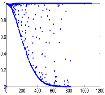
Recently, we have been able to construct a number of bidiagonal matrices of different dimensions for which DLASQ converges so slowly that it requires more iterations than allowed in the code. In these matrices, the diagonals are highly disordered and both the diagonal and off-diagonal entries are of massively varying orders of magnitude. Figure 1(a) shows the values of the diagonal elements of one such matrix, where the x-axis denotes the index of the diagonal elements and the y-axis denotes their values. The plot of the first 800 diagonal elements goes up and down, while the last 200 diagonal elements are nearly equal to one.

In this section, we use these difficult matrices and a random bidiagonal matrix whose entries are from Gaussian distribution to show the improvements of our modifications. There are five main modifications over DLASQ. Consequently we have five versions of improved algorithms by adding the new techniques one by one. We use the following notation to denote them,

• V1: d-deflation strategy in section 4.1;

• V2: new deflation strategies in section 4.2;

• V3: updating the upper bound;

• V4: twisted shift in last 20 rows;

• V5: using suitable 2-by-2 submatrix.

Table 1: The difficult bidiagonal matrices

	$n$	Description of the bidiagonal matrix $B$	Source
1	544	Matrix_1	[10]
2	1000	Matrix_2	[10]
3	1087	Matrix_3	[10]
4	1088	Matrix_4	[10]
5	5000	random bidiagonal matrix

V$i$ denotes a version after adding a new technique to the previous version. Thus V5 is the best improved algorithm. Note that the technique setting negligible $d_{\min}$ to zero has been implemented in LAPACK-3.4.1, and V1 performs similarly to the DLASQ in LAPACK-3.4.1. Table 2 shows the speedups of V5 over DLASQ in terms of time. The average iterations of V5 for each singular value are shown in Table 3. From the tables we can see that V5 requires far fewer iterations and is about 3x-10x faster than DLASQ for these difficult matrices.

Table 2: The speedup of V$i$ over DLASQ

Matrix	$n$	DLASQ	V1	V2	V3	V4	V5
1	544	1.00	1.62	1.75	2.14	2.10	2.83
2	1000	1.00	1.76	1.76	1.80	2.06	2.74
3	1087	1.00	4.98	5.20	7.88	7.88	9.99
4	1088	1.00	1.79	2.14	2.41	2.52	3.31
5	5000	1.00	1.04	1.04	1.07	1.14	1.20

Table 3: The average iterations for each singular value

Matrix	1	2	3	4	5
DLASQ	45.4	26.0	74.8	30.7	10.5
V5	11.81	7.19	7.62	8.85	7.78

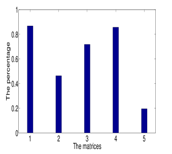
This superior performance of V5 is largely due to the d-deflation strategy in section 4.1, which is almost ‘tailor-made’ for such difficult matrices. It can deflate $40\%$-$80\%$ singular values of such matrices (see Figure 1(b).) It is also very interesting to note that it usually can deflate about $20\%$ of singular values of a general bidiagonal matrix.

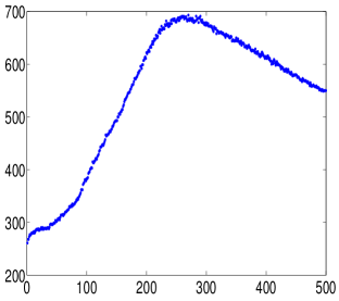
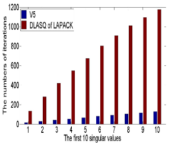
For the Matrix_3, Figure 2(a) shows the locations of negligible $d_{\min}$ when finding the first 500 singular values, which are all deflated by the d-deflation strategy. For this matrix, V5 achieves about 10x speedup. We compare the number of iterations when finding the first 10 singular values of Matrix$\_3$. The results are shown in Figure 2(b). For the first 10 singular values, DLASQ takes 120 iterations on average.

The last four improvements aim to accelerate the convergence for general bidiagonal matrices. From Table 2, we can see that each of these techniques improves the performance. Since different matrices may have very different properties, we can not expect these techniques to help a lot for all matrices. We further use all the matrices in stetester [11] to test each improvement by adding them one by one. Each technique is helpful for most of these matrices. Due to space limitations, we do not include all these results.

(a) The values of diagonal elements of Matrix_3

(b) The percentage of singular values deflated by d-deflation strategy in section 4.1

Fig. 1: Results for these difficult matrices

(a) The locations of $d_{\min}$ when finding the first 500 singular values

(b) The number of iterations for the first 10 singular values

Fig. 2: More results for Matrix_3 in Table 1

6.2 Some more tests

To further show the improvement of V5, we use some more matrices to test our algorithm. These matrices can be divided into two classes: 1) matrices from applications; 2) matrices constructed for testing the dqds algorithm.

These matrices are illustrated in Table 4. The last four are from industrial applications which are collected in LAPACK tester stetester and can be obtained from a website maintained by O. Marques [10]. To measure the computing time accurately, we intentionally choose some big matrices.

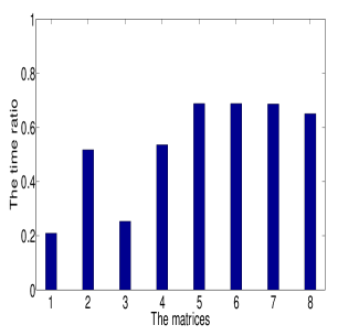
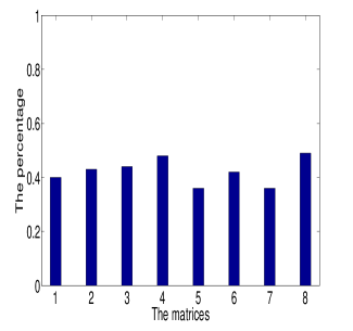
The results are shown in Figure 3(a) and Figure 3(b). Figure 3(a) shows the ratios over DLASQ in terms of time. For these matrices from industrial applications V5 saves about 30% in time. For these glued matrices which are difficult for the dqds algorithm, V5 has even more speedups, about 2x–5x times faster. Figure 3(b) provides more information. For these matrices, d-deflation strategy deflates about 40% of all singular values. Figure 3(b) further supports our conclusion that the d-deflation strategy greatly improves the performance of the dqds algorithm.

Table 4: More bidiagonal matrices

	$n$	Description of the bidiagonal matrix $B$	Source
1	15,005	Cholesky factor of Glued Wilkinson matrix	[11]
2	15,005	Cholesky factor of Glued Clement matrix	[11]
3	30,010	Cholesky factor of Glued Wilkinson matrix	[11]
4	30,010	Cholesky factor of Glued Clement matrix	[11]
5	2901	Cholesky factor of T_nasa2910_1.dat	[10]
6	3258	Cholesky factor of T_bcsstkm10_3.dat	[10]
7	4098	Cholesky factor of T_sts4098_1.dat	[10]
8	5472	Cholesky factor of T_nasa1824_3.dat	[10]

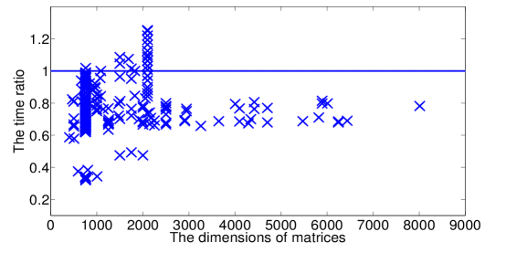
For these 254 matrices in stetester for which DLASQ needs more than $1.5e$-$2$ second, V5 usually saved about 20% in time, and was slower than DLASQ only for 32 of them but never slower than DLASQ by more than $0.0145$ second. Among these 254 matrices, V5 was 3x faster for 4 of them; 2x faster for 14 of them; 1.5x faster for 47 of them; 1.2x faster for 174 of them. The results are shown in Figure 4.

(a) The time ratio of V5 over DLASQ

(b) The percentage of singular values deflated by d-deflation strategy in section 4.1

Fig. 3: More results for matrices from construction and industry

Fig. 4: The time of V5 vs DLASQ for matrices in LAPACK tester

6.3 The test of accuracy

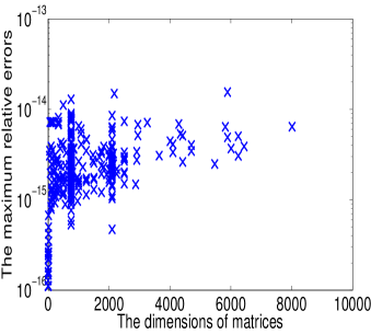
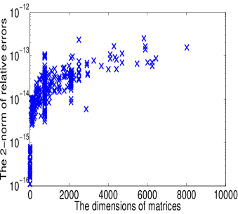
To show the accuracy of the singular values computed by our algorithm, we compared the singular values obtained by our algorithm with those gotten from a bisection algorithm. We first change the singular value problem of a bidiagonal matrix into the eigenvalue problem of a tridiagonal matrix of double size with zero diagonals, and then use a bisection algorithm to find its eigenvalues. We assume the eigenvalues computed by the bisection algorithm are ‘correct’. The results of maximum relative error are shown in Figure 5(a). Figure 5(b) shows the 2-norm of the relative errors.

(a) Maximum relative error

(b) 2-norm error

Fig. 5: The comparison of accuracy with bisection

6.4 Comparisons with aggressive early deflation

The aggressive early deflation strategy [12] is designed to enhance the dqds algorithm. This deflation strategy can help a lot for matrices which are easy for dqds. In this subsection, we demonstrate that AED does not help for those difficult matrices in Table 1. There are two versions of AED in [12], denoted by AggDef1 and AggDef2, see [12] for details. Since AggDef2 is more efficient than AggDef1 [12], we only compare our algorithms with AggDef2.

When comparing the accuracy, we also assume the results by the bisection method are correct. From the results in Table 5, we can see that for these difficult matrices AggDef2 has nearly the same performance as DLASQ. Our improved algorithm (V5) is the most accurate and fastest among these three versions.

Table 5: Comparison of V5 with AggDef2 [12] for matrices in Table 1

	Methods	Matrix_1	Matrix_2	Matrix_3	Matrix_4	Matrix_5
$n$		544	1000	1087	1088	5000
Speedup	AggDef2	1.06	1.05	1.01	1.08	1.02
$\frac{Time(DLASQ)}{Time(method)}$	V5	2.83	2.74	9.99	3.31	1.20
Max. Rel.	DLASQ	6.22e-15	9.54e-15	4.07e-14	2.42e-14	9.47e-15
	AggDef2	6.66e-15	9.33e-15	3.97e-14	2.35e-14	9.52e-15
Error	V5	3.66e-15	7.99e-15	3.85e-15	5.66e-15	6.27e-15

By combining our improvements with AggDef2, we obtain a hybrid algorithm, HDLASQ, which is summarized in Algorithm 6.4, similar to the algorithm in [12].

Algorithm 8. [HDLASQ] Inputs: bidiagonal matrix $B\in R^{n\times n}$, deflation frequency $p$ 1. while size of current segment $B$ is larger than $\sqrt{n}$ do 2. run $p$ iterations of dqds by calling V5; 3. perform aggressive early deflation; 4. end while 5. run dqds until all singular values are computed.

As mentioned in [12], setting $p$ too large may deteriorate the rate of convergence, but the performance depends not much on $p$. For example, HDLASQ with $p=200$ was about 10% slower than letting $p=20$ for matrices in Table 6 (except Mat1 for which AggDef2 is particularly effective). In our implementation, we let $p=50$.

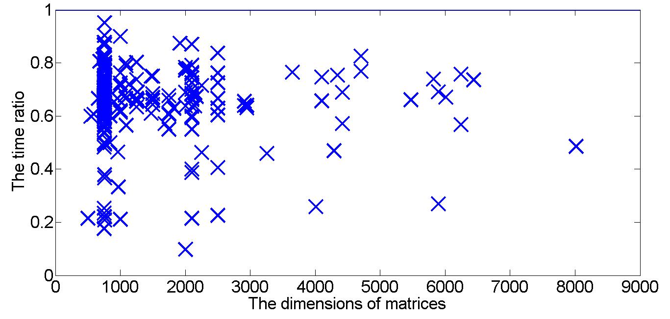
For these disordered matrices in Table 1, HDLASQ has nearly the same performance as V5. For the matrices that are good for AED (shown in Table 6), the comparison results of HDLASQ with other methods are shown in Table 7, from which we can see that HDLASQ is faster than AggDef2, DLASQ and V5. Furthermore, Figure 6 shows the time ratio of HDLASQ over DLASQ for matrices in stetester for which DLASQ needs more than $1.5e$-$2$ second. By comparing Figure 6 with Figure 4, we can also see that HDLASQ is usually better than V5.

Table 6: Some bidiagonal matrices for testing HDLASQ

Matrix	$n$	Description of the bidiagonal matrix $B$	Source
Mat1	30000	$\sqrt{q_{i}}=n+1-i,\sqrt{e_{i}}=1$	[12]
Mat2	30000	$\sqrt{q_{i}}=n+1-i,\sqrt{e_{i}}=\sqrt{q_{i}}/5$	[12]
Mat3	30000	Toeplitz: $\sqrt{q_{i}}=1$, $\sqrt{e_{i}}=2$	[11, 12]
Mat4	30000	Cholesky factor of tridiagonal (1,2,1) matrix	[11, 5]

Table 7: The comparisons of HDLASQ with AggDef2 and V5 for matrices in Table 6

	Methods	Mat1	Mat2	Mat3	Mat4
$n$		30000	30000	30000	30000
Speedup	V5	1.66	1.48	1.39	1.40
$\frac{Time(DLASQ)}{Time(method)}$	AggDef2	76.1	1.99	1.57	1.59
	HDLASQ	79.5	2.18	1.67	1.69

Fig. 6: The time of HDLASQ vs DLASQ for matrices in LAPACK tester

7 Conclusions

In this paper we first propose a novel deflation strategy for the dqds algorithm, named d-deflation strategy, which is different from the classic deflation strategies and greatly improves the dqds algorithm. Note that the shifts for the dqds algorithm must be a fraction of the upper bound $sup$. Together with the technique of updating the upper bound, they ensure the linear worst case complexity of our improved dqds algorithm V5. Additional modifications to certain shift strategies are also included. These improvements together make V5 up to 10x faster for those difficult matrices and 1.2x-4x faster in general without any loss of accuracy. By combining V5 with AED, we propose a hybrid algorithm (HDLASQ) which is shown to be faster than DLASQ, V5 and AggDef2.

In this Appendix, we prove Theorem 4.6. Our techniques are similar to those used in [1] to prove the order of convergence of the Johnson shift. We assume that matrix $B$ is defined as in (1) and that its entries satisfy $a_{k}=\sqrt{q_{k}}=\sqrt{q_{k}^{(0)}}$, $b_{k}=\sqrt{e_{k}}=\sqrt{e_{k}^{(0)}}$. In the following context, let $\{q_{k}^{(l)},e_{k}^{(l)}\}$ denote the array after $l$ dqds transforms.

We first introduce the reverse stationary differential qd algorithm with shifts (dstqds), which starts from the bottom $q_{n}$, illustrated as follows [12]. Let $\{\overset{o}{q},\overset{o}{e}\}$ denote the array after doing one dstqds transform on the $\{q,e\}$ array.

Algorithm 9. [reverse dstqds] $t_{n}=-s$ for $i=n-1,n-2,\ldots,1$ $\overset{o}{q}_{i+1}=q_{i+1}+t_{i+1}$ $tmp=\frac{e_{i}}{\overset{o}{q}_{i+1}}$ $\overset{o}{e}_{i}=q_{i+1}*tmp$ $t_{i}=t_{i+1}*tmp-s$ end for $\overset{o}{q}_{1}=q_{1}+t_{1}$

For the $\{q,e\}$ array, if we do the dqds transformation starting from $q_{1}$ and dstqds starting from $q_{n}$, there is enough information to form the twisted factorization at any $k$ we choose (see [4] for details):

$$BB^{T}-sI=\mathcal{N}\mathcal{N}^{T},$$ (15)

where

$$\mathcal{N}^{T}=\begin{bmatrix}\sqrt{q_{1}^{(1)}}&\sqrt{e_{1}^{(1)}}&&&&&&\\ &\cdotp&\cdotp&&&&\\ &0&\sqrt{q_{k-1}^{(1)}}&\sqrt{e_{k-1}^{(1)}}&&&&\\ &&0&\sqrt{\gamma_{k}}&&&&\\ &&&\sqrt{\overset{o}{e}_{k}}&\sqrt{\overset{o}{q}_{k+1}}&0&&\\ &&&&\cdotp&\cdotp&\\ &&&&&\sqrt{\overset{o}{e}_{n-1}}&\sqrt{\overset{o}{q}_{n}}\end{bmatrix},$$

and $\gamma_{k}=d_{k}+t_{k+1}\frac{e_{k}}{\overset{o}{q}_{k+1}}$.

Recall that ${\bf e}_{k}$ denotes the $k$-th column of an $n\times n$ identity matrix (to distinguish from $e_{k}$). The solution to $\mathcal{N}\mathcal{N}^{T}z^{(1)}=\gamma_{k}{\bf e}_{k}$ can be computed by

$$z^{(1)}(j)=\left\{\begin{array}[]{ll}1&\mbox{if}\quad j=k,\cr-z^{(1)}(j+1)\sqrt{e_{j}^{(1)}/q_{j}^{(1)}},&\mbox{if}\quad j<k,\\ -z^{(1)}(j-1)\sqrt{\overset{o}{e}_{j-1}/\overset{o}{q}_{j}},&\mbox{if}\quad j>k.\end{array}\right.$$ (16)

Denote $(\varphi^{(1)})^{2}=\|z^{(1)}\|^{2}-1$. By Theorem 4.5.1 [14] (or equation (12) in [16]), the smallest eigenvalue of $BB^{T}-sI$ is bounded below by

$$\phi=\gamma_{k}\frac{1-\varphi^{(1)}}{1+(\varphi^{(1)})^{2}},$$ (17)

which is used as the shift for the next dqds transform in DLASQ if $\varphi^{(1)}$ is small (for example, less than $\frac{3}{4}$). The equation (16) only needs to be solved approximately, see section 6.3.3 of [16] for details.

Below we show that for sufficiently large $l$ the shifts are chosen by the twisted shift strategy, and then prove its order of convergence. We introduce a result from [1], which states the convergence of the dqds algorithm.

Lemma .7 (Convergence of the dqds algorithm [1]).

Suppose the matrix $B$ defined as in (1) has positive nonzero elements, and the shift in the dqds algorithm is taken so that $0\leq s^{(l)}<(\sigma_{\min}^{(l)})^{2}$ holds. Then

$$\sum_{l=0}^{\infty}s^{(l)}\leq\sigma_{n}^{2}.$$ (18)

Moreover,

$$\lim_{l\rightarrow\infty} e_{k}^{(l)}=0\quad(k=1,2,\cdots,n-1),$$ (19)

$$\lim_{l\rightarrow\infty} \frac{e_{k}^{(l+1)}}{e_{k}^{(l)}}=\rho_{k},\quad(k=1,\cdots,n-1),$$ (20)

$$\lim_{l\rightarrow\infty} q_{k}^{(l)}=\sigma_{k}^{2}-\sum_{l=0}^{\infty}s^{(l)}\quad(k=1,2,\cdots,n),$$ (21)

where $\rho_{k}=\frac{\sigma_{k+1}^{2}-\sum_{l=0}^{\infty}s^{(l)}}{\sigma_{k}^{2}-\sum_{l=0}^{\infty}s^{(l)}}$.

Remark .8.

Since $\sigma_{k+1}^{2}<\sigma_{k}^{2}$ and $\rho_{k}=\frac{\sigma_{k+1}^{2}-\sum_{l=0}^{\infty}s^{(l)}}{\sigma_{k}^{2}-\sum_{l=0}^{\infty}s^{(l)}}$, we have $\rho_{k}<1$ and therefore ${e_{k}^{(l+1)}}<{e_{k}^{(l)}}$ for all large enough $l$.

Based on Lemma .7, we can prove the following lemma.

Lemma .9.

Under the same assumptions as in Lemma .7, for all sufficiently large $l$, the shifts will be chosen by the twisted shift strategy,

$$s^{(l)}=\gamma_{n}^{(l)}\frac{1-\varphi^{(l)}}{1+(\varphi^{(l)})^{2}},$$ (22)

where $\gamma_{n}^{(l)}=d_{\min}^{(l)}=q_{n}^{(l)}$ and $\varphi^{(l)}$ can be computed by (16).

Proof .10.

By [5] the smallest singular value of $B$ in (1) satisfies $\sigma_{n}>0$. By equations (19) and (21), we know that $e_{k}^{(l)}\rightarrow 0$, $q_{k}^{(l)}\geq\sigma_{k}^{2}-\sigma_{n}^{2}>0$ (as $l\rightarrow\infty$ for $k=1,2,\cdots,n-1$) and that $\{q_{k}^{(l)}\}$ gradually become monotonic with respect to $k$. For sufficiently large $l$ we will have dmink$=n$. By (16), we get

$$\begin{split}z^{(l)}(n)&=1,\\ z^{(l)}(j)&=-z^{(l)}(j+1)\sqrt{{e}_{j}^{(l)}/{q}_{j}^{(l)}},j<n.\end{split}$$ (23)

Let $(z^{(l)})^{T}=((x^{(l)})^{T}\quad 1)$ and then, after some algebraic manipulations,

$$(\varphi^{(l)})^{2}=\|x^{(l)}\|^{2}=\frac{e_{n-1}^{(l)}}{q_{n-1}^{(l)}}(1+\frac{e_{n-2}^{(l)}}{q_{n-2}^{(l)}}(1+\frac{e_{n-3}^{(l)}}{q_{n-3}^{(l)}}(1+\cdots))).$$ (24)

By equations (19) and (21), we know that $e_{k}^{(l)}\rightarrow 0$, $q_{k}^{(l)}$ converges to a positive constant as $l\rightarrow\infty$ (for $1\leq k\leq n-1$) and that $\varphi^{(l)}$ also converges to zero. Therefore, the shifts would be chosen by (22) for all sufficiently large $l$.

Remark .11.

If $\varphi^{(l)}\leq\frac{3}{4}$, DLASQ will use (22) as a shift. To prove the main conclusion of this appendix, we assume that $d_{\min}$ always moves to the bottom. The aim is analyzing the asymptotic convergence rate of the twisted shift strategy. The following lemma reveals another good property of the twisted shift. It is said that $d_{\min}=q_{n}^{(l)}$ always converges to zero if using the twisted shift.

Lemma .12.

Under the same assumptions as in Lemma .7, we have

$$\sum_{l=0}^{\infty}s^{(l)}=\sigma_{n}^{2},$$

$$\lim_{l\rightarrow\infty}q_{k}^{(l)}=\sigma_{k}^{2}-\sigma_{n}^{2}\quad(k=1,\cdots,n-1);\lim_{l\rightarrow\infty}q_{n}^{(l)}=0.$$

Proof .13.

From Lemma .9, we know $\|x^{(l)}\|\rightarrow 0$ and

$$\lim_{l\rightarrow\infty}s^{(l)}=\lim_{l\rightarrow\infty}q_{n}^{(l)}\geq 0.$$

Furthermore, since $\lim_{l\rightarrow\infty}s^{(l)}=0$ from equation (18), we have $\lim_{l\rightarrow\infty}q_{n}^{(l)}=0.$ The first two equations follow from $\lim_{l\rightarrow\infty}q_{n}^{(l)}=0$ and equation (21).

We are now ready to prove Theorem 4.6.

Proof .14.

By Algorithm 2, we have

$$\begin{split}q_{n}^{(l+1)}&=d_{n-1}^{(l+1)}\frac{q_{n}^{(l)}}{q_{n-1}^{(l+1)}}-s^{(l)}=q_{n}^{(l)}-e_{n-1}^{(l)}\frac{q_{n}^{(l)}}{q_{n-1}^{(l+1)}}-s^{(l)}\\ &=q_{n}^{(l)}-e_{n-1}^{(l+1)}-s^{(l)}.\end{split}$$

By Lemma .9 the shift is chosen by the twisted shift strategy for sufficiently large $l$, and we have

$$\begin{split}q_{n}^{(l+1)}&=q_{n}^{(l)}-e_{n-1}^{(l+1)}-q_{n}^{(l)}\frac{1-\varphi^{(l)}}{1+(\varphi^{(l)})^{2}}\\ &=q_{n}^{(l)}\frac{(\varphi^{(l)})^{2}+\varphi^{(l)}}{1+(\varphi^{(l)})^{2}}-e_{n-1}^{(l+1)},\end{split}$$

where $\varphi^{(l)}=\|x^{(l)}\|=\sqrt{\frac{e_{n-1}^{(l)}}{q_{n-1}^{(l)}}}\cdotp\sqrt{1+\xi^{(l)}},$ and $\xi^{(l)}\to 0$ as $l\rightarrow\infty$ (by equation (24)).

Hence

$$q_{n}^{(l+1)}=q_{n}^{(l)}\sqrt{e_{n-1}^{(l)}}\frac{\left(1+\|x^{(l)}\|\right)\sqrt{1+\xi^{(l)}}}{\left(1+\|x^{(l)}\|^{2}\right)\sqrt{q_{n-1}^{(l)}}}-e_{n-1}^{(l+1)}.$$ (25)

On the other hand, from the fourth line of Algorithm 2 we also have

$$e_{n-1}^{(l+2)}=\frac{q_{n}^{(l+1)}e_{n-1}^{(l+1)}}{q_{n-1}^{(l+2)}},$$

which implies

$$q_{n}^{(l+1)}=\frac{e_{n-1}^{(l+2)}q_{n-1}^{(l+2)}}{e_{n-1}^{(l+1)}}\quad\mbox{and}\quad q_{n}^{(l)}=\frac{e_{n-1}^{(l+1)}q_{n-1}^{(l+1)}}{e_{n-1}^{(l)}}.$$

Plugging these equations into (25), we obtain

$${\displaystyle\frac{e_{n-1}^{(l+2)}q_{n-1}^{(l+2)}}{e_{n-1}^{(l+1)}}=\frac{e_{n-1}^{(l+1)}q_{n-1}^{(l+1)}}{\sqrt{e_{n-1}^{(l)}}}\frac{\left(1+\|x^{(l)}\|\right)\sqrt{1+\xi^{(l)}}}{\left(1+\|x^{(l)}\|^{2}\right)\sqrt{q_{n-1}^{(l)}}}-e_{n-1}^{(l+1)},}$$ (26)

which can be rewritten as

$${\displaystyle\frac{e_{n-1}^{(l+2)}}{(e_{n-1}^{(l+1)})^{3/2}}=\eta^{(l)},}$$

with

$${\displaystyle\eta^{(l)}=\frac{\sqrt{q_{n-1}^{(l+1)}}}{q_{n-1}^{(l+2)}}\left(\frac{\sqrt{q_{n}^{(l)}}\left(1+\|x^{(l)}\|\right)\sqrt{1+\xi^{(l)}}}{\left(1+\|x^{(l)}\|^{2}\right)\sqrt{q_{n-1}^{(l)}}}-\frac{\sqrt{e_{n-1}^{(l+1)}}}{\sqrt{q_{n-1}^{(l+1)}}}\right).}$$

Since $\sqrt{1+\xi^{(l)}}\frac{1+\|x^{(l)}\|}{1+\|x^{(l)}\|^{2}}\rightarrow 1$, $e_{n-1}^{(l+1)}\rightarrow 0$, $q_{n}^{(l)}\rightarrow 0$, and $q_{n-1}^{(l+2)}$ converges to $\sigma_{n-1}^{2}-\sigma_{n}^{2}>0$, it follows that $\eta^{(l)}$ converges to $0$ as well.

References

- [1] K. Aishima, T. Matsuo, K. Murota, and M. Sugihara. On convergence of the dqds algorithm for singular value computation. SIAM J. Matrix Anal. Appl., 30:522–537, 2008.
- [2] R. P Brent. Algorithms for Minimization Without Derivatives. Prentice-Hall, the University of Michigan, 1972.
- [3] J. W. Demmel and W. M. Kahan. Accurate singular values of bidiagonal matrices. SIAM J. Sci. Comput., 11:873–912, 1990.
- [4] I. S. Dhillon and B. N. Parlett. Orthogonal eigenvectors and relative gaps. SIAM J. Matrix Anal. Appl., 25:858–899, 2004.
- [5] K. V. Fernando and B. N. Parlett. Accurate singular values and differential qd algorithms. Numer. Math., 67:191–229, 1994.
- [6] C. Ferreiva. The unsymmetric tridiagonal eigenvalue problem. PhD thesis, Univ. of Minho, Portngal, 2007.
- [7] G. H. Golub and C. F. Van Loan. Matrix Computations. The Johns Hopkins University Press, Baltimore, MD, 3rd edition, 1996.
- [8] R. Horn and C. Johnson. Topics in Matrix Analysis. Cambridge University Press, Cambridge, 1991.
- [9] W. Kahan. Personal communication, 2012.
-
[10]
O. Marques.
Osni Marques’s homepage,
http://crd-legacy.lbl.gov/~osni/. - [11] O. A. Marques, C. Voemel, J. W. Demmel, and B. N. Parlett. Algorithm 880: A testing infrastructure for symmetric tridiagonal eigensolvers. ACM Trans. Math. Softw., 35, 2008.
- [12] Y. Nakatsukasa, K. Aishima, and I. Yamazaki. dqds with aggressive early deflation. SIAM J. Matrix Anal. Appl., 33:22–51, 2012.
- [13] B. N. Parlett. The new qd algorithms. Acta Numer., 4:459–491, 1995.
- [14] B. N. Parlett. The Symmetric Eigenvalue Problem. SIAM, Philadelphia, 1998.
- [15] B. N. Parlett and M. Gutknecht. From qd to LR, or how were the qd and LR algorithms discovered? IMA Journal of Numerical Analysis, 31:741–754, 2011.
- [16] B. N. Parlett and O. Marques. An implementation of the dqds algorithm (positive case). Linear Algebra Appl., 309:217–259, 2000.
- [17] R. C. Whaley, A. Petitet, and J. J. Dongarra. Automated empirical optimizations of software and the ATLAS project. Parallel Computing, 27:3–35, 2001.
- [18] G. Wilkins and M. Gu. A modified Brent’s method for finding zeros of functions. Numer. Math., 123:177–188, 2012.