Decreasing the temporal complexity for
nonlinear, implicit
reduced-order models by forecasting
Abstract
Implicit numerical integration of nonlinear ODEs requires solving a system of nonlinear algebraic equations at each time step. Each of these systems is often solved by a Newton-like method, which incurs a sequence of linear-system solves. Most model-reduction techniques for nonlinear ODEs exploit knowledge of system’s spatial behavior to reduce the computational complexity of each linear-system solve. However, the number of linear-system solves for the reduced-order simulation often remains roughly the same as that for the full-order simulation.
We propose exploiting knowledge of the model’s temporal behavior to 1) forecast the unknown variable of the reduced-order system of nonlinear equations at future time steps, and 2) use this forecast as an initial guess for the Newton-like solver during the reduced-order-model simulation. To compute the forecast, we propose using the Gappy POD technique. The goal is to generate an accurate initial guess so that the Newton solver requires many fewer iterations to converge, thereby decreasing the number of linear-system solves in the reduced-order-model simulation.
keywords:
nonlinear model reduction , Gappy POD , temporal correlation , forecasting , initial guess1 Introduction
High-fidelity physics-based numerical simulation has become an indispensable engineering tool across a wide range of disciplines. Unfortunately, such simulations often bear an extremely large computational cost due to the large-scale, nonlinear nature of many high-fidelity models. When an implicit integrator is employed to advance the solution in time (as is often essential, e.g., for stiff problems) this large cost arises from the need to solve a sequence of high-dimensional systems of nonlinear algebraic equations—one at each time step. As a result, individual simulations can take weeks or months to complete, even when high-performance computing resources are available. This renders such simulations impractical for time-critical and many-query applications. For example, uncertainty-quantification applications (e.g., Bayesian inference problems) call for hundreds or thousands of simulations (i.e., forward solves) to be completed in days or weeks; in-the-field analysis (e.g., guidance in-field data acquisition) requires near-real-time simulation.
Projection-based nonlinear model-reduction techniques have been successfully applied to decrease the computational cost of high-fidelity simulation while retaining high levels of accuracy. To accomplish this, these methods exploit knowledge of the system’s dominant spatial behavior—as observed during ‘training simulations’ conducted a priori—to decrease the simulation’s spatial complexity, which we define as the computational cost of each linear-system solve.222A sequence of linear systems arises at each time step when a Newton-like method is employed to solve the system of nonlinear algebraic equations. To do so, these methods 1) decrease the dimensionality of the linear systems by projection, and 2) approximate vector-valued nonlinear functions by sampling methods that compute only a few of the vector’s entries (e.g., empirical interpolation [1, 2], Gappy POD [3]). However, these techniques are often insufficient to adequately reduce the computational cost of the simulation. For example, Ref. [4] presented results for the GNAT nonlinear model-reduction technique applied to a large-scale nonlinear turbulent-flow problem. The reduced-order model generated solutions with sub-1% errors, reduced the spatial complexity by a factor of 637, and employed only 4 computing cores—a significant reduction from the 512 cores required for the high-fidelity simulation. However, the total number of linear-system solves required for the reduced-order-model simulation, which we define as the temporal complexity, remained large. In fact, the temporal complexity was decreased by a factor of only 1.5. As a result, the total computing resources (computing cores wall time) required for the simulation were decreased by a factor of 438, but the wall time was reduced by a factor of merely 6.9. While these results are promising (especially in their ability to reduce spatial complexity), the time integration of nonlinear dynamics remains problematic and often precludes real-time performance.
The goal of this work is exploit knowledge of the system’s temporal behavior as observed during the training simulations to decrease the temporal complexity of reduced-order-model simulations. For this purpose, we first briefly review methods that exploit observed temporal behavior to improve computational performance.
Temporal forecasting techniques have been investigated for many years with a specific focus on reducing wall time in a stable manner with maximal accuracy. The associated body of work is large and a comprehensive review is beyond the scope of this paper. However, this work focuses on time integration for reduced-order models of highly nonlinear dynamical systems; several categories of specialized research efforts provide an appropriate context for this research.
At the most fundamental level of temporal forecasting, a variety of statistical time-series-analysis methods exist that exploit 1) knowledge of the temporal structure, e.g., smoothness, of a model’s variables, and 2) previous values of these variables for the current time series or trajectory. The connection between these methods and our work is that such forecasts can serve as an initial guess for an iterative solver (e.g., Newton’s method) at an advanced point in time. However, the disconnect between such methods and the present context is that randomness and uncertainty drive time-series analysis; as such, these forecasting methods are stochastic in nature (see Refs. [5, 6, 7, 8, 9, 10, 11, 12]). In addition, the majority of time-series analyses have been applied to application domains (e.g., economics) with dynamics that are not generally modeled using partial differential equations. Finally, such forecasting techniques do not exploit a collection of observed, complete time histories from training experiments conducted a priori. Because such training simulations lend important insight into the spatial and temporal behavior of the model, we are interested in developing a technique that can exploit such data.
Alternatively, time integrators for ordinary differential equations (ODEs) employ polynomial extrapolations to provide reasonably accurate forecasts of the state or the unknown at each time step. Time integrators employ such a forecast for two purposes. First, algorithms with adaptive time steps employ interpolation to obtain solutions (and their time derivatives) at arbitrary points in time. Implicit time integrators for nonlinear ODEs, which require the iterative solution of nonlinear algebraic systems at each time step, use recent history (of the current trajectory) to forecast an accurate guess of the unknown in the algebraic system (see, e.g., Ref. [13]). Again, forecasting by polynomial extrapolation makes no use of the temporal behavior observed during training simulations.
Closely connected to time integration but specialized to leverage developments in high-performance computing, time parallel methods can offer computational speedup when integrating ODEs. Dating back to before the general availability of parallel computers, researchers speculated about the benefits of decomposing the temporal domain across multiple processors [14]. Advancements have been made from parallel multigrid to parareal techniques [15, 16, 17, 18]. Although time-domain decomposition algorithms have demonstrated speedup, they are limited in comparison to the spatial domain decomposition methods and they require a careful balance between stability and computational efficiency [19]. It is possible that these methods could further improve performance in a model-reduction setting [20] (and could complement the method proposed in this work), but near real-time performance is likely unachievable through time-parallel methods alone.
To some extent, exploiting temporal behavior has been explored in nonlinear model reduction. Bos et al. [21] proposed a reduced-order model in the context of explicit time integration wherein the generalized coordinates are computed based on a best-linear-unbiased (BLU) estimate approach. Here, the reduced state coordinates at time step are computed using empirically derived correlations between the reduced state coordinates and 1) their value at the previous time step, 2) the forcing input at the previous time step, and 3) a subset of the full-order state. However, the errors incurred by this time-integration procedure (compared with standard time integration of the reduced-order model) are not assessed or controlled. This can be problematic in realistic scenarios, where error estimators and bounds are essential. Another class of techniques known as a priori model reduction methods [22, 23] build a reduced-order model ‘on the fly’, i.e., over the course of a given time integration. These techniques aim to use the reduced-order model at as many time steps as possible; they revert to the high-fidelity model when the reduced-order model is deemed to be inaccurate. In effect, these techniques employ the reduced-order model as a tool to accelerate the high-fidelity-model simulation. In contrast, this work aims to accelerate the reduced-order-model simulation itself. Further, these methods differ from the present context in that there are no training experiments conducted a priori from which to glean insight into the model’s temporal behavior.
In this work, we propose a method that exploits a set of complete trajectories observed during training simulations to decrease the temporal complexity of a reduced-order-model simulation. The method 1) forecasts the unknown variable in the reduced-order system of nonlinear algebraic equations, and 2) uses this forecast as an initial guess for the Newton-like solver. To compute the forecast, the method employs the Gappy POD method [3], which extrapolates the unknown variable at future time steps by exploiting the unknown variable for the previous time steps (where can be interpreted as the memory of the process), and a database of time histories of the unknown variable. If the forecast is accurate, then the Newton-like solver will require very few iterations to converge, thereby decreasing the number of linear-system solves needed for the simulation. The method is straightforward to implement: the (offline) training stage simply requires collecting an additional set of snapshots during the training simulations. In some scenarios, no additional offline work is required. The (online) reduced-order-model simulation simply requires an external routine for determining the initial guess for the Newton-like solver.
2 Problem formulation
This section provides the context for this work. Section 2.1 describes the class of full-order models we consider, which includes first- and second-order ODEs numerically solved by implicit time integration. Section 2.2 describes the reduced-order modeling strategies for which the proposed technique is applicable.
2.1 Full-order model
2.1.1 First- and second-order ODEs
First, consider the parameterized nonlinear first-order ODE corresponding to the full-order model of a dynamical system:
| (1) | |||
| (2) |
Here, time is denoted by , the time-dependent forcing inputs are denoted by , the time-independent parametric inputs are denoted by with denoting the parameter domain, and is nonlinear in at least its first argument. The state is denoted by with denoting the number of degrees of freedom in the model. The parameterized initial condition is .
Because this work addresses both first- and second-order ODEs, consider also the parameterized nonlinear second-order ODE corresponding to the full-order model of a dynamical system:
| (3) | |||
| (4) | |||
| (5) |
Here, the function is nonlinear in at least its first or second argument, and the parameterized initial velocity is denoted by .333Note that an -dimensional second-order ODE can be rewritten as -dimensional first-order ODE.
2.1.2 Implicit time integration
Given forcing and parametric inputs, the numerical solution to the full-order model described by Eqs. (1)–(2) or (3)–(5) can be computed via numerical integration. For stiff systems, an implicit integration method is often the most computationally efficient choice; it is even essential in many cases [24]. When an implicit time integrator is employed, coupled -dimensional systems of nonlinear algebraic equations are solved at each time step , where denotes the total number of time steps:
| (6) |
Here, the function is nonlinear in at least one of its first arguments and the unknowns , are implicitly defined by (6). As discussed in A and B, the unknowns represent the state, velocity, or acceleration at points , where is defined by the time integrator:
| (7) |
Thus, a superscript denotes the value of a quantity at time , a superscript denotes the value of a quantity at time , and denotes the time-step size.
After the unknowns are computed by solving Eq. (6), the state is explicitly updated as
| (8) |
where and , are scalars defined by the integrator. For second-order ODEs, the velocity is also updated explicitly as
| (9) |
where and , are also scalars defined by the integrator. A and B specify the form of Eqs. (6)–(9) for important classes of implicit numerical integrators for first- and second-order ODEs, respectively.
The chief computational burden of solving Eq. (1) with an implicit integrator lies in solving nonlinear equations (6) at each time step; this is typically done with a Newton-like method. In particular, if denotes the average number of Newton-like iterations required to solve (6), then the full-order-model simulation requires solving linear systems of dimension .444Assuming the Jacobian of the residual is sparse with an average number of nonzeros per row , the dominant computational cost of solving Eqs. (6) for the entire simulation is if a direct linear solver is used. It is if an iterative linear solver is used. Here, denotes the average number of matrix-vector products required to solve each linear system in the case of an iterative linear solver. We denote the simulation’s spatial complexity to be the computational cost of solving each linear system; we consider the simulation’s temporal complexity to be the total number of linear-system solves.
The spatial complexity contributes significantly to the computational burden for large-scale systems because is large. However, the temporal complexity is also significant for such problems. First, the number of total time steps is often proportional to a fractional power of . This occurs because refining the mesh in space often necessitates a decrease in the time-step size to balance the spatial and temporal errors.555This is not necessarily true for explicit time-integration schemes, when the time-step size is limited by stability rather than accuracy. In this case, Krysl et al. [25] showed that employing a low-dimensional subspace for the state may improve stability and therefore permit a larger time-step size. As a result, the reduced-order state equations can be solved fewer times than the full-order state equations. Second, the average number of Newton-like iterations can be large when the problem is highly nonlinear and large time steps are taken, which is common for implicit integrators. Under these conditions, the initial guess for the Newton solver, which is often taken to be a polynomial extrapolation of the unknown, can be far from the true value of the unknown.
In many cases (e.g., linear multi-step methods, single-stage Runge–Kutta schemes), . For this reason, and for the sake of notational clarity, the remainder of this paper assumes , and designates the value of the unknown variable at time . However, we note that the proposed technique can be straightforwardly extended to .
2.2 Reduced-order model
Nonlinear model-reduction techniques aim to generate a low-dimensional model that is inexpensive to evaluate, yet captures key features of the full-order model. To do so, these methods first perform analyses of the full-order model for a set of training parametric and forcing points during a computationally intensive ‘offline’ training stage. These analyses may include integrating the equations of motion, modal decomposition, etc.
Then, the data generated during these analyses are employed to decrease the the cost of each linear-system solve via two approximations: 1) dimensionality reduction, 2) nonlinear-function approximation (spatial-complexity reduction). Once these approximations are defined, the resulting reduced-order model is employed to perform computationally inexpensive analyses for any inputs during the ‘online’ stage.
2.2.1 Dimensionality reduction
Model-reduction techniques decrease the number of degrees of freedom by computing an approximate state that lies in an affine trial subspace of dimension :
| (10) | |||
| (11) | |||
| (12) |
Here, the trial basis (in matrix form) is denoted by with . The generalized state is denoted by . The reference state is , which is often set to zero. The initial condition for the reduced-order model is obtained by projecting the full-order-model initial condition onto this affine subspace such that
| (13) | |||
| (14) |
When the unknown variable computed at each time step (see Section 2.1.2) corresponds to the state, velocity, or acceleration, this dimensionality reduction for the state results in the following dimensionality reduction for the unknown:
| (15) |
where if the unknown is the state and otherwise, and denotes the vector of generalized unknowns.
Substituting Eqs. (10)–(11) into (1) yields
| (16) |
Alternatively, substituting Eq. (10)–(12) into (3) yields
| (17) |
The overdetermined ODEs described by (16) and (17) may not be solvable, because and in general. Several methods exist to compute an approximate solution.
Project, then discretize in time
This class of model-reduction methods first carries out a projection process on the ODE followed by a time-integration of the resulting low-dimensional ODE. The (Petrov–Galerkin) projection process enforces orthogonality of the residual corresponding to the overdetermined ODE (16) or (17) to an -dimensional test subspace , with . Assuming is invertible, this leads to the following for first-order ODEs:
| (18) |
For second-order ODEs, the result is
| (19) |
Galerkin projection corresponds to the case where .
Because Eq. (18) (resp. (19)) is an ODE of the same form as (1) (resp. (3)), it can be solved using the same numerical integrator that was used to solve Eq. (1) (resp. (3)). Further, the same time-step sizes are often employed, as the time-step size is determined by accuracy (not stability) for implicit time integrators. For both first- and second-order ODEs, this again leads to a system of nonlinear equations to be solved at each time step :
| (20) |
The unknown can be computed by applying Newton’s method to (20). Then, the explicit updates (8)–(9) can proceed as usual to compute the resulting state.
Discretize in time, then project
This class of model-reduction techniques first applies the same numerical integrator that was used to solve (1) to the overdetermined ODE (16) or (17). However, the resulting algebraic system of nonlinear equations in unknowns remains overdetermined:
| (21) |
To compute a unique solution to Eq. (21), orthogonality of the discrete residual to a test subspace can be enforced. However, this leads to a reduced system of nonlinear equations equivalent to (20). So, in this case, the two classes of model-reduction techniques are equivalent.
On the other hand, to compute a unique solution to (21), the discrete-residual norm can be minimized [26, 4, 27, 28, 29], which ensures discrete optimality [4]:
| (22) |
The unknown can be computed by applying a Newton-like nonlinear least-squares method (e.g., Gauss–Newton, Levenberg–Marquardt) to problem (22). Again, explicit updates for the state (8)–(9) can proceed after the unknowns are computed.
2.2.2 Spatial-complexity reduction
For nonlinear dynamical systems, the dimensionality reduction described in Section 2.2.1 is insufficient to guarantee a reduction in the computational cost of each linear-system solve. The reason is that the full-order residual depends on the state, so it must be recomputed and subsequently projected or minimized at each Newton-like iteration.
For this reason, nonlinear model-reduction techniques employ a procedure to reduce the spatial-complexity, i.e., decrease the computational cost of computing and projecting or minimizing the nonlinear residual. Such techniques are occasionally referred to as ‘hyper-reduction’ techniques [22]. In particular, the class of ‘function sampling’ techniques replace the full-order nonlinear residual with an approximation that is inexpensive to compute. Then, is employed in (20) or (22) to compute the unknowns .
Methods in this class can be categorized as follows:
- 1.
-
2.
Function-reconstruction approaches. These methods employ a residual approximation that computes a few entries of the residual or nonlinear function, and subsequently ‘fills in’ the remaining entries via interpolation or least-squares regression. That is, these methods apply one of the following approximations:
(24) (25) (26) Here, , , and are empirically derived bases used to approximate the nonlinear residual, velocity, and acceleration, respectively. A superscript denotes the Moore–Penrose pseudoinverse. When the bases are computed via POD, this technique is known as Gappy POD [3]. This approach has been developed for Galerkin projection [30, 21, 2, 31, 32] and discrete-residual minimization [26, 4]. In particular, the discrete empirical interpolation (DEIM) method [2] is a specific case of Gappy POD for first-order ODEs, Galerkin projection, and the interpolatory case, i.e., DEIM uses approximation (25) in Eq. (18) with and sets the number of sample indices equal to the number of columns in the matrix . The GNAT method [26, 4] employs Gappy POD of the residual in a discrete residual minimization setting, i.e., GNAT uses approximation (24) in Eq. (22).
3 Temporal-complexity reduction
While the model-reduction approaches described in the previous section decrease the computational cost of each linear-system solve (i.e., spatial complexity), they do not necessarily decrease the number of linear-system solves (i.e., temporal complexity). The goal of this work is devise a method that decreases this temporal complexity while introducing no additional error.
3.1 Method overview
The main idea of the proposed approach is to compute an accurate forecast of the generalized unknowns at future time steps using the Gappy POD procedure, and employ this forecast as an initial guess for the Newton-like solver at future time steps.
Gappy POD is a technique to reconstruct vector-valued data that has ‘gaps,’ i.e., entries with unknown or uncomputed values. Mathematically, the approach is equivalent to least-squares regression in one discrete-valued variable using empirically computed basis functions. It was introduced by Everson and Sirovich [3] for the purpose of image reconstruction. It has also been used for static [33, 34] and time-dependent [35, 36] flow field reconstruction, inverse design [34], design variable mapping for multi-fidelity optimization [37], and for decreasing the spatial complexity in nonlinear model reduction [30, 21, 26, 4]. This work proposes a novel application of Gappy POD: as a method for forecasting the generalized unknown at future time steps during a reduced-order-model simulation.
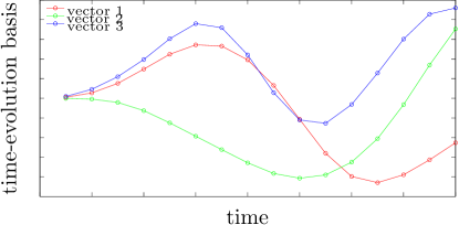
During the offline stage, the proposed method computes a ‘time-evolution basis’ for each generalized unknown , . Each basis represents the complete time-evolution of a generalized unknown as observed during training simulations. Figure 1(a) depicts this idea graphically, and Section 3.2 describes a computationally inexpensive way to compute these bases.
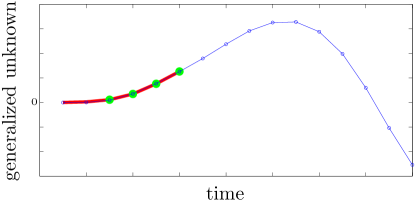
During the online stage, the method computes a forecast of the generalized unknowns at future time steps via Gappy POD. This forecast employs 1) the time-evolution bases and 2) the generalized unknowns computed at several previous time steps. Figure 1(b) depicts this, and Section 3.3 describes the forecasting method in detail. At future time steps, this forecast is employed as an initial guess for the Newton-like solver. If the forecast is accurate, the Newton-like solver will converge in very few iterations; if it is inaccurate, the Newton-like solver will require more iterations for convergence. Note that the accuracy of the solution is not hampered in either case (assuming a globalization strategy is employed). If the number of Newton iterations required for convergence is large, this indicates an inaccurate initial guess. When this occurs, the method computes a new forecast using the most recently computed generalized unknowns.
The proposed method is expected to be effective if 1) the temporal behavior of the generalized unknowns is similar across input variation and 2) the original model is not too weakly nonlinear at each time step. The latter issue can hamper the proposed method’s performance because it is difficult to reduce the number of Newton iterations if the original number is already very small. This situation can occur, for example, if the simulation employs a very small time step. However, this is uncommon for (unconditionally stable) implicit time integrators, where taking the largest time step while maintaining accuracy is typically the most computationally efficient approach.
The proposed method is independent of the dimensionality-reduction or spatial-complexity-reduction scheme employed by the reduced-order model; further, the method is applicable (without modification) to both first- and second-order ODEs. The next sections describe the offline and online steps of the methodology in detail.
3.2 Offline stage: compute the time-evolution bases
The objective of the offline stage is to compute the time-evolution bases that will be used for the online forecast. Ideally, the bases should be able to describe the time evolution of the generalized state for any forcing inputs and parametric inputs . If the bases are ‘bad’, then the forecasting step of the algorithm will be inaccurate, and there may be no reduction in the average number of Newton-like iterations.
We propose employing a POD basis for the time evolution of the generalized unknown. This basis is computed a priori during ‘offline’ simulations of the reduced-order model in three steps:
-
1.
Collect snapshots of the unknown during each of the training simulations:
(27) for , with . Here, denotes the forcing inputs for training simulation , and denotes the parametric inputs for training simulation .
-
2.
Compute the corresponding snapshots of the generalized unknown:
(28) (29) for , where orthogonality of the trial basis has been used. Here, and denotes a vector of ones.
-
3.
Compute the time-evolution bases via the (thin) singular value decomposition (SVD). Defining the th column of as , , we note that can be interpreted as a snapshot of the time evolution of the th generalized unknown during training simulation . Then, this step amounts to
(30) (31) for . Here, and .
After the time-evolution bases , have been computed during the offline stage, they can be used to accelerate online computations via forecasting. The next section describes this.
-
Remark. In some cases, many of the above offline steps are already completed as part of the existing model-reduction process. For example, the snapshot matrices , in Step 1 are already available if proper orthogonal decomposition (POD) is employed to compute and the time integrator’s unknown is the state (e.g., linear multistep schemes). If additionally and the POD basis is computed via the SVD of the reference-centered state snapshots, i.e., with , , then of Step 2 is already available as . Here, the square bracket indicates a submatrix over the specified range of row and column indices and . Further, in this case the matrices in Step 3 are also available as , , where .
3.3 Online stage: forecast
During the online stage, the method employs a forecasting procedure to define the initial guess for the Newton-like solver. To compute this forecast, it uses the time evolution bases (computed offline), and the values of the generalized unknown at the previous time steps (computed online). Here, is considered the ‘memory’ of the process. Because the forecast is defined at all time steps (see the blue curve in Figure 1(b)), it is used as the initial guess at future time steps until the number of Newton iterations exceeds a threshold value . This indicates a poor forecast. In this case, the forecast is recomputed using the most recent values of the generalized unknown.
If the forecast is accurate, then the number of iterations needed to converge from the (improved) initial guess will be drastically reduced, thereby decreasing and hence the temporal complexity. Algorithm 1 outlines the proposed technique.
To compute the forecasting coefficients in step 11 of Algorithm 1, we propose using the Gappy POD approach introduced by Everson and Sirovich [3]. This approach computes coefficients via the following linear least-squares problem:
| (32) |
Here, the matrix is the sampling matrix that selects entries corresponding to the previous time steps:
| (33) |
where denotes the th canonical unit vector. Note that is required for Eq. (32) to have a unique solution. The function in (32) ‘unrolls’ time according to the time discretization; we define with as
| (34) |
The online cost to compute this forecast is very small, as it entails solving small-scale linear least-squares problem (32) characterized by a matrix. For this reason, it is generally advantageous to employ a small value of (i.e., 0 or 1), which results in a frequent (inexpensive) recomputation of the forecast.
4 Numerical experiments
These numerical experiments assess the performance of the proposed temporal-complexity-reduction method on a structural-dynamics example using three reduced-order models: Galerkin projection (Eq. (19) with ), Galerkin projection with least-squares reconstruction of the residual (Eq. (24)), and a structure-preserving reduced-order model [38]. We do not present results for a collocation ROM (see Eq. (23)), as this approach was unstable in most cases, even when 60% of the degrees of freedom were selected as sample indices (i.e., ). Section 4.1 provides a description of the problem—a parameterized, damped clamped–free truss structure subjected to external forces—and details the experimental setup. We then consider a sequence of problems that poses increasing difficulty to the method.
Section 4.2 considers the ideal scenario for the method: the online points are identical to the training points, and the reduced bases are not truncated. In this case, the temporal behavior of the system is perfectly predictable, because (in exact arithmetic) the online response is the same as the training response. Therefore, we expect the proposed method to work extremely well.
Section 4.3 assesses the method’s performance in a more challenging setting. Here, the online points differ from the training points (i.e., a predictive scenario), so the temporal behavior is not identical to that observed during the training simulations. The parametric inputs correspond to shape parameters and the initial displacement. The external force is set to zero, which leads to a damped free-vibration problem. As a result, the dynamics encountered in this example are relatively smooth.
Section 4.4 considers a more challenging predictive scenario wherein rich dynamics—generated from a high-frequency external force—characterize the response. Here, additional parametric inputs are considered, which correspond to the magnitudes and frequencies of the high-frequency forces.
Section 4.5 increases the predictive difficulty, as the allowable range of the parametric inputs is doubled, leading to a more significant variation in the responses.
Finally, Section 4.6 summarizes the proposed forecasting method’s performance over all experiments and tested reduced-order models.
4.1 Problem description
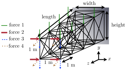
Figure 2 depicts the parameterized, non-conservative clamped–free truss structure we consider. The truss is parameterized by parametric inputs that affect the geometry, initial condition, and applied force as described in Table 1.
| length (m) | bar | width (m) | height (m) | initial condition | external-force | external-force |
| cross-sectional | max magnitude (N) | magnitude | frequency | |||
| area () | , | , | , | |||
We set the material properties to those of aluminum, i.e., density and elastic modulus Pa. The external force is composed of four components:
| (35) |
where , correspond to unit loads uniformly distributed across designated nodes and , denote the forcing inputs. Figure 2 depicts the spatial distribution of the forces, which lead to vectors , through the finite-element formulation described below. The parameterized, time-dependent magnitudes of these forces are
| (36) |
where and , denote the maximum force magnitudes and force frequencies, respectively. Similarly, the initial displacement is composed of four components where is the steady-state displacement of the truss subjected to load with denoting the nominal point in parameter space. The initial velocity is set to zero , and the reference configuration is simply the undeformed truss (in equilibrium) represented by .
The problem is discretized by the finite-element method. The model consists of 16 three-dimensional bar elements per bay with three degrees of freedom per node; this results in 12 degrees of freedom per bay. We consider a problem with 250 bays, and therefore degrees of freedom in the full-order model. The bar elements model geometric nonlinearity, which results in a high-order nonlinearity in the internal force. This discretization results in the following equations of motion for the full-order model:
| (37) |
Here, denotes the symmetric-positive-definite mass matrix, the internal force is denoted by , and the symmetric-positive-semidefinite Rayleigh viscous damping matrix, denoted by , is of the form
| (38) |
Note that represents the tangent stiffness matrix at the initial condition. Here, and are chosen such that the damping ratio is for the uncoupled ODEs associated with the smallest two eigenvalues of the matrix pencil [39].
The equations of motion (37) can be rewritten in the standard form of Eqs. (3)–(5) as
| (39) | |||
| (40) | |||
| (41) |
The nonlinear function defining the acceleration for the second-order ODE is then
| (42) |
We employ an implicit Nyström time integrator with constant timestep size , to compute the numerical solution to Eqs. (39)–(41) in the time interval with seconds. In particular, we employ the implicit midpoint rule for both partitions. This leads to discrete equations (58) to be solved at each time step with explicit updates (59)–(60) and parameters , , , , , . The unknowns are equivalent to the acceleration at the half time steps: , . Multiplying the corresponding residual by yields
| (43) |
To solve at each time step, We employ a globalized Newton solver with a More–Thuente linesearch [40]. Except when noted, convergence of the Newton iterations is declared when the residual norm reaches of its value computed using a zero acceleration and the values of the displacement and velocity at the beginning of the timestep. The linear system arising at each Newton iteration is solved directly.
The experiments compare the performance of three reduced-order models: Galerkin projection (Eq. (20) with ), Galerkin projection with Gappy POD residual approximation (Eq. (24)), and a model-reduction method based that preserves the classical Lagrangian structure intrinsic to the problem (Ref. [38], proposal 1). To construct the reduced-order models, we collect snapshots of the required quantities for and . The trial basis is determined via POD. We collect snapshots of the state
| (44) |
and set the trial basis to , where is an ‘energy criterion’ and is defined by Algorithm 2 in C. The reference state is set to , as this is the equilibrium state for this problem [38]. For Galerkin projection with least-squares (Gappy POD) residual reconstruction, the following snapshots are collected during the (full-order model) training simulations:
| (45) |
Here, denotes the number of Newton steps taken at time step . The residual basis is set to with . For the structure-preserving method, we also collect snapshots of both the mass matrix and the external forcing vector:
| (46) | |||
| (47) |
The POD basis for the external force employed by the structure-preserving method is set to with
Reduced-order models with spatial-complexity reduction employ the same sampling matrix , which is generated using GNAT’s greedy sample-mesh algorithm [4, Algorithm 3].666Greedy-algorithm parameters are a POD basis computed using Algorithm 2 with snapshots of the numerical residual over all timesteps and Newton iterations during the full-order-model training simulations and an energy criterion of , a target number of sample nodes with unknowns per node (the -, -, and -displacements), an empty seeded sample-node set , and equal to the number of columns in . These models are also implemented using the sample-mesh concept [4, Section 5]. For the structure-preserving method [38], we solve the reduced-basis-sparsification unconstrained optimization problem using the Poblano toolbox [40].777The initial guess for each of these problems is chosen as .
In all experiments, the proposed forecasting method employs untruncated time-evolution bases: , . We compare its performance with that of the most common approach for generating an initial guess: a polynomial extrapolation of varying degree. Note that polynomial extrapolations of different degrees employ a different number of previous solutions to generate an initial guess; in our experiments, we associate the number of previous solutions employed with a ‘memory’ . For example, a zeroth-order extrapolation requires the previous solution (), so in this case. When no previous solution is used (i.e., ), the polynomial-extrapolation approach uses . In all experiments, the full-order model employs a zeroth-order extrapolation for the initial guess.
The output of interest is the -displacement of the bottom-left node of the end face of the truss in Figure 2. We denote this (parameterized, time-dependent) quantity by . To quantify the performance of the reduced-order models, the following metrics are used:
| (48) | |||
| (49) | |||
| (50) |
Here, error measure designates the scaled norm of the discrepancy in the output predicted by a reduced-order model. The temporal-complexity-reduction factor is denoted by , where denotes the average number of Newton-like steps taken per time step over the course of a simulation. The speedup is denoted by with T denoting the wall time required for a simulation. A subscript ‘FOM’ denotes a quantity computed using the full-order model.
All computations are carried out in Matlab on a Mac Pro with 2 2.93 GHz 6-Core Intel Xeon processors and 64 GB of memory.
4.2 Ideal case: unforced, invariant inputs, no truncation of bases
This experiment explores the ideal case for the method: the online inputs equal the training inputs, and the bases are not truncated (). The resulting basis dimensions are for the reduced basis and for the residual basis (i.e., ). In this scenario, the full-order model’s temporal behavior encountered online is exactly the same as that observed during training simulation; for this reason, we expect the proposed method to perform very well. We consider a single configuration () characterized by , with no applied forcing , . The nominal forces that affect the initial condition (see Table 1) are set to and . The time-step size is set to seconds, leading to total time steps. This value was determined by a timestep-verification study using a timestep-refinement factor of two; a timestep of seconds led to an approximated rate of convergence in the output quantity at the end of the time interval of (which is reasonably close to the scheme’s asymptotic rate of convergence of 2.0) and an approximated error in this quantity (computed via Richardson extrapolation) of .
We assess the performance of the ROMs with spatial-complexity reduction (i.e., Gappy POD and the structure-preserving ROM) using two different sets of sample indices. First, we set the number of sample nodes equal to 20% of the total nodes in the mesh (i.e., ), which leads to . We also employ a sampling fraction of 5%, which leads to . For the forecasting technique, the Newton-step threshold is set to and the maximum memory is set to . For the ‘no forecasting’ case, we employ a zeroth-order polynomial extrapolation. For experiments in this section, we declare the Newton iterations to have converged when the residual norm reaches of its value computed using a zero acceleration and the values of the displacement and velocity at the beginning of the timestep.
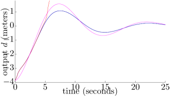
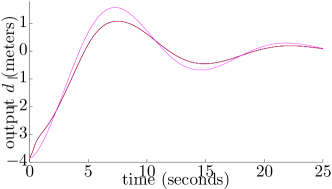
The full-order-model simulation consumed minutes and incurred Newton iterations (). Table 2 and Figure 3 report the results for the reduced-order models. First, note that the relative errors generated by Galerkin and Gappy POD ROM with 20% sampling are essentially zero. This is expected, because the reduced bases are not truncated and the inputs are fixed. Further, note that the Galerkin ROM without forecasting generates no speedup; this is expected because it is not equipped with a spatial-complexity-reduction technique (see Section 2.2.2). The other two techniques—which employ spatial-complexity-reduction approximations—lead to speedups. The exception is Gappy POD with 5% sampling, which yields an unstable response; this is depicted in Figure 3(a). For this reason, subsequent experiments employ a larger sampling fraction for the Gappy POD ROM compared with the structure-preserving ROM.
Importantly, note that the reduced-order models exhibit very little temporal-complexity reduction (i.e., ) in the absence of the proposed forecasting technique. When the models employ the proposed forecasting technique, the number of Newton iterations decreases, leading to temporal-complexity reductions of for the Galerkin ROM and and for the best-performing Gappy POD and structure-preserving ROMs, respectively. In turn, this leads to improved wall-time speedups in all cases.
The Galerkin ROM case presented here can be viewed as the best possible performance for the method (applied to this problem): the temporal behavior of the system is exactly predictable, as the inputs have not changed, and the reduced basis has not been truncated. So, the forecast is ‘perfect’ after only one time step for the Galerkin ROM. This means that for each time step after the first one, the initial guess generated by the forecasting method is equal to the solution at that time step, so no Newton steps are needed to compute the solution. As a result, no Newton iterations are carried out beyond the first time step. The next sections investigate the forecasting method’s performance in the (more realistic) case of varying inputs and truncated bases.
-
Remark. Note that the speedup (2.00) of the Galerkin ROM with forecating is not nearly as significant as the reduction factor (114.5), as Newton iterations are not the only aspect of the simulation that contribute to computational time. For example, the solution, velocity, and acceleration are updated at each time step, the residual is computed at each time step to check for convergence, outputs are computed, etc. We expect these two values to align more closely for problems where the computational cost of the Newton iterations dominates the overall simulation time.
| ROM method | sampling fraction | relative error | No forecasting | With forecasting | ||||
| Newton its | speedup | reduction factor | Newton its | speedup | reduction factor | |||
| Galerkin | - | 209 | 0.955 | 1.10 | 2 | 2.00 | 114.5 | |
| Gappy POD | 0.2 | 209 | 2.97 | 1.10 | 101 | 4.34 | 2.26 | |
| 0.05 | unstable | - | - | - | - | - | - | |
| structure preserving | 0.2 | 199 | 3.40 | 1.15 | 107 | 4.27 | 2.14 | |
| 0.05 | 199 | 12.7 | 1.15 | 102 | 16.3 | 2.25 | ||
4.3 Unforced, varying inputs
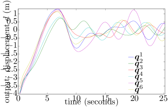
We now consider a fully predictive scenario with . Again, we set the forces to zero, which implies , . We use training points and determine using Latin hypercube sampling [41]. We randomly select two online points. Figure 4 depicts the tip displacement for the training points. As the problem setup is the same as the previous section (except for the parameter variation), we employ the same timestep size of seconds, leading to time steps.
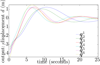
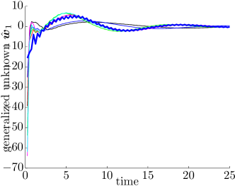
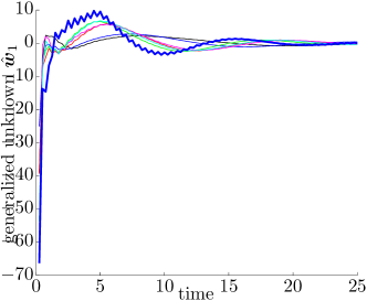
To gain insight into the proposed method’s potential, Figure 5 depicts the time evolution of the first generalized unknown —which is one of the forecasted variables—for the online and training points. Importantly, note that the qualitative response of this unknown is quite similar across parameter variation, which suggests that the forecasting method has the potential to generate accurate forecasts.
To construct the reduced-order models, we employ truncation critera of , which leads to a basis dimension of , and for Gappy POD, which results in a dimension of 316 for the residual basis. For the structure-preserving ROM, we sample 5% of the indices such that ; as this led to instabilities for Gappy POD, we sample 60% of the indices (i.e., ) for that method.
Figure 6 reports the responses of the full-order model and all three reduced-order models. The full-order-model simulation required 18.5 minutes and 307 total Newton iterations () for online point and 20.4 minutes and 347 Newton iterations () for online point . Note that the reduced-order models are very accurate at the prediction points. At online point , they generate relative errors of (Galerkin), (Gappy POD), and (structure preserving). At online point , the relative errors are (Galerkin), (Gappy POD), and (structure preserving).888Different initial guesses for the Newton solver lead to (slightly) different computed responses. Thus, the ROM responses in principle depend on the forecasting method. However, the resulting differences in errors were negligible in these experiments; therefore, we only report the ROM error generated by an initial guess of zero (i.e., polynomial forecast, in Figure 6).
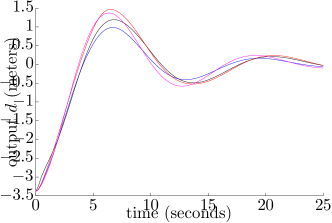
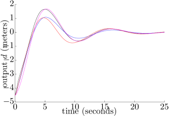
Figure 7 reports the Newton-iteration and wall-time performance of the reduced-order models for different forecasting strategies at the two online points. First, note that the proposed forecasting method always yields better performance than polynomial extrapolation, regardless of the values for the forecasting parameters or polynomial degree. Second, observe that the performance of the proposed forecasting method is relatively insensitive to its parameters and . Also, note that adding ‘memory’ to the polynomial extrapolation forecast—which yields a higher-degree extrapolant—is almost always deleterious to its performance. In addition, improvement in wall-time speedup provided by the forecasting technique is not as strong as the improvement in number of Newton iterations. This can be attributed to the presence of other operations (e.g., solution updating, residual computation to check for convergence) that contribute to the simulation time (see the remark in Section 4.2). Finally, observe that the speedups generated by the structure-preserving method are far superior to those generated by Galerkin and Gappy POD. This is due to the fact that the structure-preserving method employed only , whereas Galerkin is not equipped with a spatial-complexity-reduction mechanism and Gappy POD required to generate a stable response.
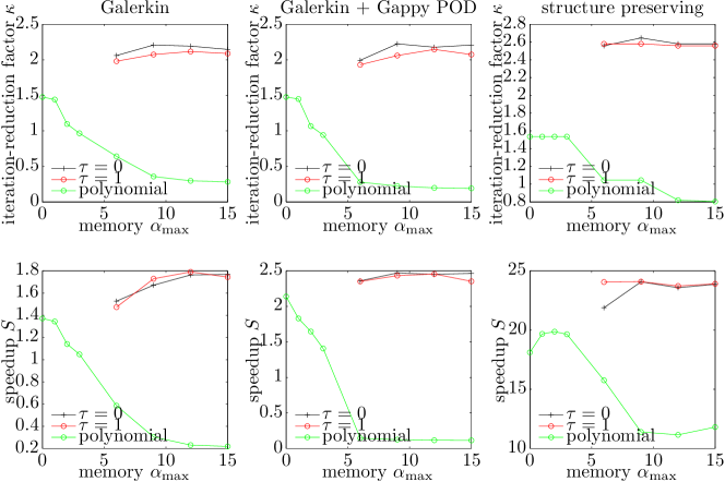
4.4 Forced, varying inputs
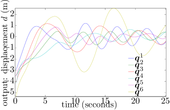
In this section, we activate the external forcing, thereby allowing , . The timestep was again set to seconds, leading to time steps. This value was again determined by a timestep-verification study at the nominal configuration using a refinement factor of two. The approximated rate of convergence in the output quantity at the end of the time interval for this timestep size was determined to be 1.67 (close to the asymptotic value of 2.0), and the error in this quantity as approximated by Richardson extrapolation was . As before, we used Latin hypercube sampling to determine the training points; Figure 8(a) reports the full-order-model responses at these points. Note that parameter variation leads to significant changes in the response. We randomly select two online points at which we will perform prediction with the ROMs.
Figure 9 depicts the time evolution of the first generalized unknown for the online and training points. As before, there is qualitative similarity of this forecasted variable for the different points; this suggests the forecasting method can again realize computational savings. Also, note that the character of the response changes appreciably when the external force is activated at seconds.
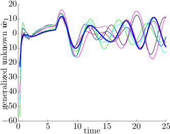
The reduced-order models employ trunction critera of (basis dimension of ) and a residual-basis dimension of 1800. The structure-preserving method approximates the external force via Gappy POD (see Ref. [38]); for this purpose, it employs a truncation criterion of , leading to a basis dimension of 4.999Note that the external force is composed of only four linearly independent components , (see Eq. (35)). Again, the Gappy POD ROM employs a sampling rate of () and the structure-preserving ROM employs a samping percentage of ().101010The Gappy POD ROM was unstable for .
Figure 10 reports the responses of the full-order model and the reduced-order models at the online prediction points. The full-order model consumed 20.3 minutes and 330 Newton iterations () at online point and 22.6 minutes and 360 Newton iterations () at point . The relative errors of the ROMs at online point are (Galerkin), (Gappy POD), and (structure-preserving). For online point , the errors are (Galerkin), (Gappy POD), and (structure-preserving). Note that the Galerkin and structure-preserving ROMs are quite accurate, but the Gappy POD ROM incurs significant errors.
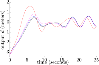
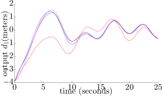
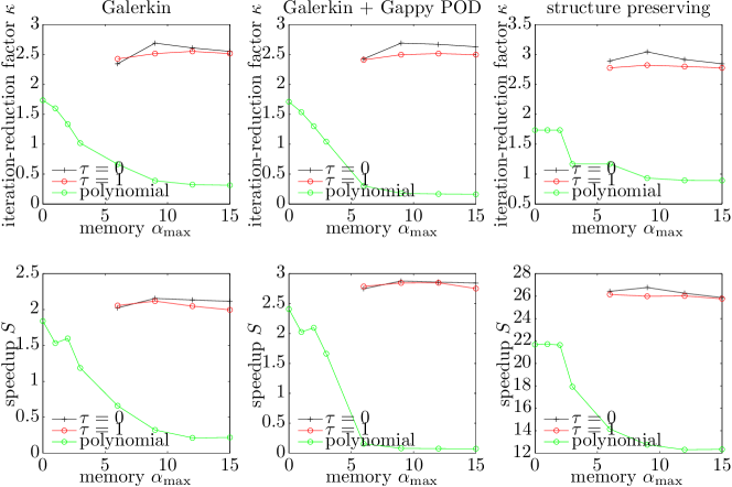
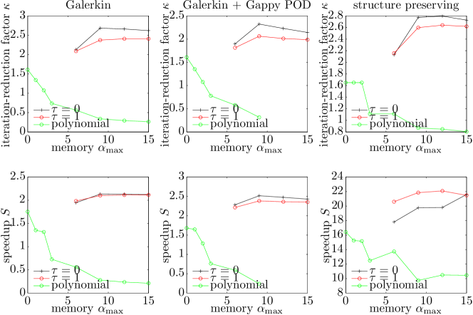
Figure 11 reports the Newton-iteration and wall-time performance of the ROMs for different forecasting strategies. The results are very similar to those for the unforced case: the proposed forecasting method nearly always exhibits performance superior to that of polynomial extrapolation, the proposed method is relatively insensitive to the parameters and , and high-order polynomial extrapolation performs very poorly. In addition, improvement in iteration-reduction factor exceeds the improvement in speedup , and the structure-preserving method generates the largest speedups due to the fact it employs the smallest number of sample indices. Additionally, notice the ‘missing’ data points for polynomial extrapolation with and for the Gappy POD ROM; these missing data indicate that the Gappy POD ROM did not converge for these forecasts. This implies that the initial guesses were so poor that the globalized Newton method failed to generate an acceptable solution within the alloted 500 Newton iterations at least one time step.
Also, note that employing appears to systematically outperform in terms of the iteration-reduction factor metric. However, this does not always lead to an improvement in speedup (see the structure-preserving ROM for ). This can be attributed to the fact that employing results in more frequent forecast recomputation (i.e., whenever the number of Newton iterations exceeds zero) than the case.
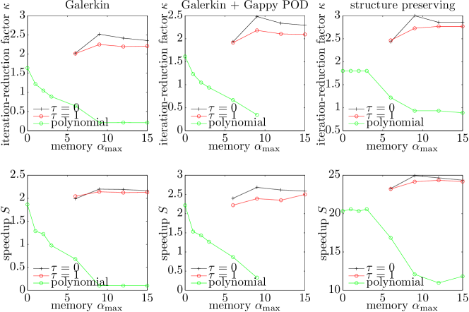
These results highlight that the proposed forecasting method is applicable even for the more challenging problem of parameterized forced responses.
4.5 Forced, varying inputs, larger parameter variation.
In this section, we assess the performance of the method for the same problem as Section 4.4, but with an increased parameter variation, i.e., . This poses a greater challenge for both the reduced-order models and the forecasting method, as they now rely on training data from the same number of points (we keep ) in a larger parameter domain. As the model now undergoes larger parameter variation, we decrease the timestep size to seconds, leading to total time steps.111111The full-order model did not converge for several of the training points when seconds was employed. Note that this timestep remains in the asymptotic range of convergence for the nominal configuration , as it is smaller than the previously verified value of 0.25 seconds. Again, training points are chosen by Latin hypercube sampling, and the online points are selected randomly. Figure 8(b) reports the full-order-model responses at the training points; note that the changes in the response are in fact more significant than for the previous case with smaller parameter variation.
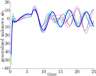
Figure 12 again reports the time evolution of the first generalized unknown. Note that again there is similar qualitative structure across parameter variation.
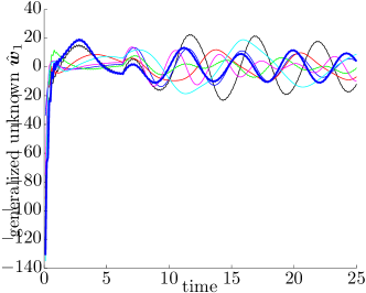
The attributes for the reduced-order models are the same as in Section 4.4, with one exception: a criterion of is employed for the state, which associates with a basis dimension of . Note that basis dimension is larger than in the previous case.
Figure 13 depicts the full-order-model response along with those for the reduced-order models. The full-order model took 36.7 minutes and 605 Newton iterations () at online point and 37.3 minutes and 595 Newton iterations () at point . As before, the Galerkin and structure-preserving ROMs are more accurate than the Gappy POD ROMs. The relative errors at point are (Galerkin), (Gappy POD), and (structure preserving). At online point , the associated errors are (Galerkin), (Gappy POD), and (structure preserving).
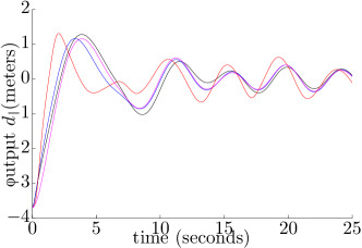
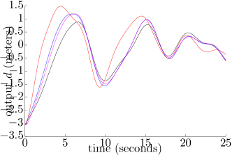
Figure 14 reports the Newton-iteration and wall-time results for the different forecasting strategies. Note that the results are extremely similar to those in Section 4.4. The primary exception can be seen by comparing Figure 14 with 11: the iteration-reduction factor and speedup performance of the reduced-order models has decreased. This can be attributed to the challenge of larger parameter variation, as the ROMs are now responsible for capturing a wider range of physics.
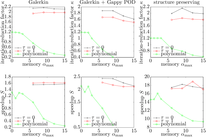
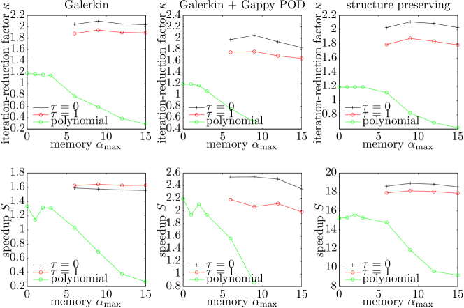
From this set of experiments, we conclude that the proposed technique can improve ROM performance even for problems with relatively large parameter variation.
4.6 Average performance
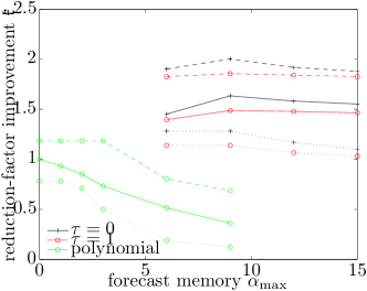
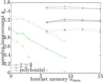
Finally, we summarize the performance of the forecasting techniques over the complete set of experiments. Figure 15 reports average, minimum, and maximum values of the reduction-factor improvement , and speedup improvement over all experiments (i.e., all three experiments in Sections 4.3–4.5, all three reduced-order models, and both online points and ). Here, and can each be computed for a given ROM simulation; a subscript ‘no’ indicates the value of the variable for a zero initial guess (i.e., polynomial extrapolation with ). First, note that the proposed method always outperforms polynomial forecasting in the mean, maximum, and minimum achieved performance for both reduction-factor improvement and speedup improvement . Secondly, the maximum, minimum, and average performance of polynomial forecasting were all made worse by increasing the polynomial degree.
Finally, the best average performance was achieved for a forecast memory of and Newton-iteration criterion of . In this case, the iteration-reduction factor was increased by on average; the speedup was improved by on average. Critically, note that these temporal-complexity gains incur no additional error, and so they strictly serve to improve the performance of the ROMs with no penalty.
5 Conclusions
This paper has described a method for decreasing the temporal complexity of nonlinear reduced-order models in the case of implicit time integration. The method exploits knowledge of the dynamical system’s temporal behavior in the form of ‘time-evolution bases’; one such basis is generated for each generalized coordinate of the time integrator’s unknown during the (offline) training stage. During the (online) deployed stage, these time-evolution bases are used—along with the solution at recent time steps—to forecast the unknown at future time steps via Gappy POD. If this forecast is accurate, the Newton-like solver will converge in very few iterations, leading to computational-cost savings.
Numerical experiments demonstrated the potential of the method to significantly improve the performance of nonlinear reduced-order models, even in the presence of high-frequency content in the dynamics. The experiments also demonstrated the effect of input parameters on the method’s performance, and provided a parameter study to analyze the effect of the method’s parameters.
Future work includes devising a way to directly handle frequency and phase shifts in the response, as well as time-shifted temporal behavior.
Acknowledgments
The authors acknowledge Julien Cortial for providing the original nonlinear-truss code that was modified to generate the numerical results, as well as the anonymous reviewers for their insightful suggestions.
This research was supported in part by an appointment to the Sandia National Laboratories Truman Fellowship in National Security Science and Engineering, sponsored by Sandia Corporation (a wholly owned subsidiary of Lockheed Martin Corporation) as Operator of Sandia National Laboratories under its U.S. Department of Energy Contract No. DE-AC04-94AL85000.
Appendix A Implicit time-integration schemes: first-order ODEs
For notational simplicity, consider a system without parametric inputs , and define such that
| (51) |
Further, denote by the time-step size at time step .
A.1 Implicit linear multi-step schemes
A linear -step method applied to first-order ODEs can be expressed as
| (52) |
where and is necessary for consistency. These methods are implicit if . In this case, the form of the residual is
| (53) |
and the explicit state update is simply
| (54) |
Therefore, the unknown is the state at time .
A.2 Implicit Runge–Kutta schemes
For an -stage Runge–Kutta scheme, the form of the residual is
| (55) |
with the following explicit computation of the state:
| (56) |
The unknowns correspond to the velocity at times , .
Appendix B Implicit time-integration schemes: second-order ODEs
For notational simplicity, consider a second-order differential equations without parametric inputs and define such that
| (57) |
B.1 Implicit Nyström method
Nyström methods are partitioned Runge–Kutta schemes applied to second-order ODEs. They lead to the following representation for the residuals:
| (58) | ||||
. The state and velocity are updated explicitly as
| (59) | |||
| (60) |
The unknowns correspond to the acceleration at times , .
B.2 Implicit Newmark method
The implicit Newmark method leads to the following residuals:
| (61) |
The state and velocity are explicitly updated as
| (62) | |||
| (63) |
Here, the unknown corresponds to the acceleration at time .
Appendix C Proper orthogonal decomposition
Algorithm 2 describes the method for computing a proper-orthogonal-decomposition (POD) basis given a set of snapshots. The method essentially amounts to computing the singular value decomposition of the snapshot matrix. The left singular vectors define the POD basis.
| (64) | ||||
| (65) |
References
- Barrault et al. [2004] M. Barrault, Y. Maday, N. C. Nguyen, A. T. Patera, An ‘empirical interpolation’ method: application to efficient reduced-basis discretization of partial differential equations, Comptes Rendus Mathématique Académie des Sciences 339 (2004) 667–672.
- Chaturantabut and Sorensen [2010] S. Chaturantabut, D. C. Sorensen, Nonlinear model reduction via discrete empirical interpolation, SIAM Journal on Scientific Computing 32 (2010) 2737–2764.
- Everson and Sirovich [1995] R. Everson, L. Sirovich, Karhunen–Loève procedure for gappy data, Journal of the Optical Society of America A 12 (1995) 1657–1664.
- Carlberg et al. [2013] K. Carlberg, C. Farhat, J. Cortial, D. Amsallem, The GNAT method for nonlinear model reduction: effective implementation and application to computational fluid dynamics and turbulent flows, Journal of Computational Physics 242 (2013) 623–647.
- Diggle [1990] P. Diggle, Time Series: A Biostatistical Introduction, Clarendon Press, 1990.
- Gourieroux [1997] C. Gourieroux, ARCH models and financial applications, Springer-Verlag, 1997.
- Engle [1982] R. F. Engle, Autoregressive conditional heteroscedasticity with estimates of the variance of U. K. inflation, Econometrica 50 (1982) 987–1008.
- Graybill [1961] F. A. Graybill, An introduction to linear statistical models, McGraw-Hill, New York, 1961.
- Hollander and Wolfe [1973] M. Hollander, D. A. Wolfe, Nonparametric statistical methods, Wiley, New York, 1973.
- Percival and Walden [1993] D. B. Percival, A. T. Walden, Spectral Analysis for Physical Applications, Cambridge University Press, 1993.
- Holt [2004] C. C. Holt, Forecasting seasonals and trends by exponentially weighted moving averages, International Journal of Forecasting 20 (2004) 5–10.
- Winters [1960] P. R. Winters, Forecasting sales by exponentially weighted moving averages, Management Science 6 (1960) 324–342.
- Brown et al. [1989] P. Brown, G. Byrne, A. Hindmarsh, VODE: A variable-coefficient ODE solver, SIAM Journal on Scientific and Statistical Computing 10 (1989) 1038–1051.
- Nievergelt [1964] J. Nievergelt, Parallel methods for integrating ordinary differential equations, Communications of the ACM 7 (1964) 731–733.
- Gander [1999] M. J. Gander, A waveform relaxation algorithm with overlapping splitting for reaction diffusion equations, Numerical Linear Algebra with Applications 6 (1999) 125–145.
- Horton and Vandewalle [1995] G. Horton, S. Vandewalle, A space-time multigrid methods for parabolic partial differential equaions, SIAM J. Sci. Comput. 16 (1995) 848–864.
- Lions et al. [2001] J. Lions, Y. Maday, G. Turinici, A “parareal” in time discretization of PDEs, Comptes Rendus de l’Academie des Sciences Series I Mathematics 332 (2001) 661–668.
- Cortial [2011] J. Cortial, Time-parallel methods for accelerating the solution of structural dynamics problems, Ph.D. thesis, Stanford University, 2011.
- Farhat and Chandesris [2003] C. Farhat, M. Chandesris, Time-decomposed parallel time-integrators: theory and feasibility studies for fluid, structure, and fluid-structure applications, International Journal for Numerical Methods in Engineering 58 (2003) 1397–1434.
- Harden [2008] C. Harden, Real time computing with the parareal algorithm, Ph.D. thesis, Florida State University, 2008.
- Bos et al. [2004] R. Bos, X. Bombois, P. Van den Hof, Accelerating large-scale non-linear models for monitoring and control using spatial and temporal correlations, Proceedings of the American Control Conference 4 (2004) 3705–3710.
- Ryckelynck [2005] D. Ryckelynck, A priori hyperreduction method: an adaptive approach, Journal of Computational Physics 202 (2005) 346–366.
- Kim and James [2009] T. Kim, D. James, Skipping steps in deformable simulation with online model reduction, ACM Transactions on Graphics 28 (2009) 1–9.
- Hairer and Wanner [2002] E. Hairer, G. Wanner, Solving ordinary differential equations II: stiff and differential-algebraic problems, Springer Verlag, 2002.
- Krysl et al. [2001] P. Krysl, S. Lall, J. E. Marsden, Dimensional model reduction in non-linear finite elements dynamics of solids and structures, Int. J. Numer. Meth. Engng 51 (2001) 479–504.
- Carlberg et al. [2011] K. Carlberg, C. Bou-Mosleh, C. Farhat, Efficient non-linear model reduction via a least-squares Petrov–Galerkin projection and compressive tensor approximations, International Journal for Numerical Methods in Engineering 86 (2011) 155–181.
- Bui-Thanh et al. [2008a] T. Bui-Thanh, K. Willcox, O. Ghattas, Model reduction for large-scale systems with high-dimensional parametric input space, SIAM Journal on Scientific Computing 30 (2008a) 3270–3288.
- Bui-Thanh et al. [2008b] T. Bui-Thanh, K. Willcox, O. Ghattas, Parametric reduced-order models for probabilistic analysis of unsteady aerodynamic applications, AIAA Journal 46 (2008b) 2520–2529.
- LeGresley [2006] P. A. LeGresley, Application of Proper Orthogonal Decomposition (POD) to Design Decomposition Methods, Ph.D. thesis, Stanford University, 2006.
- Astrid et al. [2008] P. Astrid, S. Weiland, K. Willcox, T. Backx, Missing point estimation in models described by proper orthogonal decomposition, IEEE Transactions on Automatic Control 53 (2008) 2237–2251.
- Galbally et al. [2009] D. Galbally, K. Fidkowski, K. Willcox, O. Ghattas, Non-linear model reduction for uncertainty quantification in large-scale inverse problems, International Journal for Numerical Methods in Engineering 81 (2009) 1581–1608.
- Drohmann et al. [2012] M. Drohmann, B. Haasdonk, M. Ohlberger, Reduced basis approximation for nonlinear parametrized evolution equations based on empirical operator interpolation, SIAM Journal on Scientific Computing 34 (2012) A937–A969.
- Bui-Thanh et al. [2003] T. Bui-Thanh, D. Murali, K. Willcox, Proper orthogonal decomposition extensions for parametric applications in compressible aerodynamics, AIAA Paper 2003-4213, 21st Applied Aerodynamics Conference, Orlando, FL (2003).
- Bui-Thanh et al. [2004] T. Bui-Thanh, M. Damodaran, K. Willcox, Aerodynamic data reconstruction and inverse design using proper orthogonal decomposition, AIAA Journal 42 (2004) 1505–1516.
- Venturi and Karniadakis [2004] D. Venturi, G. E. Karniadakis, Gappy data and reconstruction procedures for flow past a cylinder, Journal of Fluid Mechanics 519 (2004) 315–336.
- Willcox [2006] K. Willcox, Unsteady flow sensing and estimation via the gappy proper orthogonal decomposition, Computers and Fluids 35 (2006) 208–226.
- Robinson et al. [2006] T. D. Robinson, M. S. Eldred, K. Willcox, R. Haimes, Strategies for multifidelity optimization with variable dimensional hierarchical models, AIAA Paper 2006-1819, 47th AIAA/ASME/ASCE/AHS/ASC Structures, Structural Dynamics, and Materials Conference, Newport, RI (2006).
- Carlberg et al. [2014] K. Carlberg, R. Tuminaro, P. Boggs, Preserving Lagrangian structure in nonlinear model reduction with application to structural dynamics, arXiv preprint 1401.8044 (2014).
- Chowdhury and Dasgupta [2003] I. Chowdhury, S. Dasgupta, Computation of Rayleigh damping coefficients for large systems, The Electronic Journal of Geotechnical Engineering 8 (2003).
- Dunlavy et al. [2010] D. Dunlavy, T. Kolda, E. Acar, Poblano v1. 0: A Matlab toolbox for gradient-based optimization, Sandia National Laboratories, Albuquerque, NM and Livermore, CA, Tech. Rep. SAND 1422 (2010).
- McKay et al. [1979] M. D. McKay, R. J. Beckman, W. J. Conover, Comparison of three methods for selecting values of input variables in the analysis of output from a computer code, Technometrics 21 (1979) 239–245.
