Q-boson coherent states and para-Grassmann variables for multi-particle states

Abstract

We describe coherent states and associated generalized Grassmann variables for a system of $m$ independent $q$-boson modes. A resolution of unity in terms of generalized Berezin integrals leads to generalized Grassmann symbolic calculus. Formulae for operator traces are given and the thermodynamic partition function for a system of $q$-boson oscillators is discussed.

I Introduction

Exclusion statistics is one possible way to generalize the pattern of bosonic or fermionic particles Gentile1940 . A creation operator $a^{\dagger}$ can create at most $k-1$ particles at a given site (or mode) by stating $k$-nilpotency: acting on a vacuum $|0\rangle$,

$$\left(a^{\dagger}\right)^{n}|0\rangle \neq 0\text{ for }n=0,\cdots,k-1$$

$$\left(a^{\dagger}\right)^{k}|0\rangle = 0.$$ (1)

Standard bosons are recovered in the limit $k\to\infty$ while the fermionic Pauli exclusion principle corresponds to $k=2$. Other ways to generalize ordinary statistics include the braiding symmetrization of the many-body system wavefunction Leinaas_1977 , the fractional exclusion principle Haldane_PRL67_1991 and modifications of the algebra of commutation/anticommutation relations of creation and annihilation operators Green_1953 ; Biedenharn_1989 .

Amongst proposals of systems satisfying integer exclusion statistics with finite $k\geq 3$, we are interested in this work in the so called $k$-nilpotent $q$-boson particles Biedenharn_1989 . We first review the operator formulation of quantum mechanics for one degree of freedom and for a system of $m$ independent $q$-boson modes. Then we discuss the construction of coherent states, for which it is necessary to introduce $k$-nilpotent para-Grassmann numbers Rausch_1988 (cf. Grassmann numbers in the fermionic case). The order of nilpotency $k$ is usually related to commutation rules for para-Grassmann numbers Filipov_1993 (in a similar way that fermionic $k=2$ nilpotency leads to anticommuting Grassmann numbers). Ordering issues are then important and have made cumbersome the manipulation of coherent states. Several authors have dealt with this problem Filipov_1993 ; Baulieu_1991 ; Filipov_1992 ; Rausch_1998 ; Lozano_2004 ; SIGMA2006 generating a variety of conventions and finding unavoidable difficulties, in particular when dealing with multiparticle states.

We explore in this work the consistency of using non-standard para-Grassmann commutation relations and a normal order convention El_Baz_2010 ; Sontz_2012 , highly simplifying the operations but still retaining the essence of exclusion statistics. We then write down a para-Grassmann symbolic expression for the trace of operators and use it to study the thermodynamics of $q$-boson systems. The partition function for non-interacting systems can be readily computed, alongside with derived quantities like the mean free energy and the specific heat, observing that $k$-nilpotent bosons interpolate the features of Fermi-Dirac and Bose-Einstein statistics.

The present formalism could be useful in the study of strongly correlated systems in low dimensions, where effective quasi-particles with exclusion statistical properties seem to be ubiquitous. The constraints on available states for spin $S$ particles, or for electrons in t-J models, or for fermionic and bosonic occupation in representations of spin operators AA , impose rules on statistical distributions which often manifest in fractional statistics. Noticeably, the fractional exclusion statistics characterized by Haldane Haldane_PRL67_1991 is realized in several strongly correlated systems in one and two dimensions like the Haldane-Shastry spin chain Haldane_PRL66_1991 and generalizations Schoutens_1994 and the Fractional Quantum Hall Effect Halperin_1984 (where fractional exclusion statistics is consistent with anyon braiding statistics Leinaas_1977 ). In one dimensional Conformal Field Theories, the underlying Yangian symmetry allows for the construction of a basis of quasi-particle excitations which also have been proved to obey of exclusion statistics Schoutens_1997 .

Other approaches to exotic statistics, not mentioned above, have been developed. One should recall the concept of quons Greenberg_1991 as particles interpolating between bosons and fermions, and the fact that nilpotent particles can be also described by $q$-fermions Parthasarathy_1991 (see for instance Chaichian_Montonen_1993 for a comparison of different approaches). Because of their potential utility, these proposals receive current attention in relation with strongly correlated systems JPA36_Avancini ; JPA44_Mirza ; JPA44_Gavrilik .

II q-boson operators

The origin of $q$-bosons finds its roots in a Schwinger-like bosonic representation of the quantum deformed $SU(2)_{q}$ generators Biedenharn_1989 , where $q$ is a real deformation parameter; later, the consideration of $q$ as a rational phase Baulieu_1991 led to nilpotent operators.

We consider in this work a set of $m$, $k$-nilpotent, independent $q$-boson modes $a_{i}$, $a_{i}^{\dagger}$ ($i=1,\cdots,m$). For each mode Baulieu_1991 ; Rausch_1998 ; SIGMA2006 $a_{i}$ is an annihilation operator and $a_{i}^{\dagger}$, its Hermitian conjugate, is the corresponding creation operator satisfying the $q$-commutation relations

$$a_{i}a_{i}^{\dagger}-qa_{i}^{\dagger}a_{i}=q^{-N_{i}},$$ (2)

and conjugate relations

$$a_{i}a_{i}^{\dagger}-q^{-1}a_{i}^{\dagger}a_{i}=q^{N_{i}},$$ (3)

where $q=e^{i\frac{\pi}{k}}$ , $k\in\mathbb{N}$, $k\geq 2$, and $N_{i}$ is a number operator that, from (2), can be related with $a_{i}$, $a_{i}^{\dagger}$ by

$$a_{i}^{\dagger}a_{i}=\frac{q^{N_{i}}-q^{-N_{i}}}{q-q^{-1}}.$$ (4)

From a vacuum vector $|0_{i}\rangle$ annihilated by $a_{i}$ one can construct a Fock space generated by the orthonormal set

$$|n_{i}\rangle=\frac{\left(a_{i}^{\dagger}\right)^{n_{i}}}{\sqrt{[n_{i}]_{q}!}}|0_{i}\rangle,\;n_{i}=0,\cdots,k-1,$$ (5)

where $[n]_{q}$ stands for the $q$-deformation of integer numbers

$$[n]_{q}\equiv\frac{q^{n}-q^{-n}}{q-q^{-1}}$$ (6)

and the factorial is defined by $[0]_{q}!\equiv 1$, $[n]_{q}!\equiv[n]_{q}[n-1]_{q}\cdots[1]_{q}$. In this representation one can readily express the action of the basic operators

$$N_{i}|n_{i}\rangle = n_{i}|n_{i}\rangle,$$

$$a_{i}^{\dagger}|n_{i}\rangle = \sqrt{[n_{i}+1]_{q}}|n_{i}+1\rangle,$$ (7)

$$a_{i}|n_{i}\rangle = \sqrt{[n_{i}]_{q}}|n_{i}-1\rangle.$$

Being $q=e^{i\frac{\pi}{k}}$ a rational phase one has

$$[n]_{q}=\frac{\sin\left(n\pi/k\right)}{\sin\left(\pi/k\right)}$$ (8)

so that $[k]_{q}=[0]_{q}=0$ and the Fock space ${\cal H}_{i}\sim\mathbb{C}^{k}$ is finite dimensional, with $\left(a_{i}\right)^{k}=\left(a_{i}^{\dagger}\right)^{k}=0$. Due to the symmetry $[n]_{q}=[k-n]_{q}$, one has $[n]_{q}![k-1-n]_{q}!=[k-1]_{q}!$ for any $n=0,\cdots,k-1$. The relations (7) are conveniently seen as finite dimensional matrix analogues of the usual harmonic oscillator (Heisenberg-Weyl) algebra, with $q$-deformed integers $[n]_{q}$ instead of integers $n$.

From the deformed algebra (2), notice that one recovers the usual commutation relations

$$[N_{i},a_{i}]=-a_{i},\hphantom{xxx}[N_{i},a_{i}^{\dagger}]=a_{i}^{\dagger},$$ (9)

reflecting that $N_{i}$ is indeed the number operator for the $i^{th}$ mode. It is simple to recover $q$-commutation relations (3) from the matrix representation, by noting that $[n+1]_{q}=q[n]_{q}+q^{-n}$.

From the above facts, the $k$-nilpotent $q$-bosons describe a simple system exhibiting exclusion statistics. They may be seen as hard core particles, with $k$ regulating the core hardness: they combine properties of bosons, but carry in their very formulation a maximum occupation constraint. It is apparent that in the limit $k\to\infty$ (i.e. $q\to 1$) one recovers standard bosons. However, the case $k=2$ does not describe fermions (see (2)).

Regarding the commutation properties for different modes, we follow the criteria that $q$-bosonic operators corresponding to different degrees of freedom commute Shabanov_1993 ; Floratos_1991 ; Chaichian_Montonen_1993 ,

$$[a_{i},a_{j}]=[a_{i}^{\dagger},a_{j}^{\dagger}]=[a_{i},a_{j}^{\dagger}]=0\hphantom{--}\text{for }i\neq j.$$ (10)

This bosonic behaviour is set even for $k=2$, another departure from fermions in our treatment. The Fock space of the system is thus simply ${\cal H}=\otimes_{i}{\cal H}_{i}$. In comparison with standard bosons, recovered in the limit $q\to 1$, one must stress that a unitary transformation $U(m)$ of $q$-bosons does not render $q$-bosonic modes Floratos_1991 .

III Coherent states - single particle case

We discuss in this section one single mode $i$. Coherent states in ${\cal H}_{i}$ may be defined as eigenvectors of $a_{i}$; however, one readily notes that the only eigenvector of $a_{i}$ in the finite dimensional space ${\cal H}_{i}$ is the vacuum, as it happens for fermionic operators. The way out is to enlarge the Hilbert space by allowing linear combinations with coefficients that go beyond the complex numbers. One is lead to introduce $k$-nilpotent para-Grassmann numbers Rausch_1988 , in the same way that Grassmann numbers are needed to deal with fermionic coherent states Ohnuki_1978 . Consider an indeterminate $\theta_{i}$ and a formal vector

$$|\theta_{i})=\sum_{n_{i}=0}^{k-1}\alpha_{n_{i}}\theta_{i}^{n_{i}}|n_{i}\rangle,$$ (11)

where $\alpha_{n_{i}}$ are complex coefficients (we introduce the notation “$|\quad)$” El_Baz_2010 to distinguish this expression from proper vectors in ${\cal H}_{i}$), and evaluate

$$a_{i}|\theta_{i})=\theta_{i}\sum_{n_{i}=0}^{k-2}\alpha_{n+1}\theta_{i}^{n_{i}}\sqrt{[n_{i}+1]_{q}}|n_{i}\rangle.$$ (12)

The conditions for having an eigenvector are

$$\alpha_{n_{i}+1}=\alpha_{n_{i}}/\sqrt{[n_{i}+1]_{q}}$$ (13)

and

$$\theta_{i}^{k}=0,$$ (14)

imposing the $k$-nilpotency condition. One then gets

$$|\theta_{i})=\sum_{n_{i}=0}^{k-1}\left(\alpha_{0}/\sqrt{[n_{i}]_{q}!}\right)\theta_{i}^{n_{i}}|n_{i}\rangle$$ (15)

satisfying

$$a_{i}|\theta_{i})=\theta_{i}|\theta_{i}).$$ (16)

Next, one introduces formal dual vectors by conjugation: consider $\bar{\theta}_{i}$ an indeterminate conjugate to $\theta_{i}$ and dual vectors $\langle n_{i}|$ in ${\cal H}_{i}^{*}$ to define

$$(\theta_{i}|=\sum_{n_{i}=0}^{k-1}\langle n_{i}|\left(\bar{\alpha}_{0}/\sqrt{[n_{i}]_{q}!}\right)\bar{\theta}_{i}^{n_{i}}$$ (17)

so that

$$(\theta_{i}|a_{i}^{\dagger}=(\theta_{i}|\bar{\theta}_{i}.$$ (18)

The action of $(\theta_{i}|$ on $|\theta_{i})$ gives a polynomial in $\theta_{i}$, $\bar{\theta}_{i}$

$$(\theta_{i}|\theta_{i})=\sum_{n_{i}=0}^{k-1}|\alpha_{0}|^{2}\frac{\bar{\theta}_{i}^{n_{i}}\theta_{i}^{n_{i}}}{[n_{i}]_{q}!}$$ (19)

which is not a real number and cannot be normalized; we adopt the convention $\alpha_{0}=1$. We remark that, up to this stage, the construction includes standard Grassmann numbers for $k=2$.

Commutation relations and conjugation

Before prescribing an iterated integration rule over $\theta_{i}$ and $\bar{\theta}_{i}$ (see below), one needs a commutation relation $\theta_{i}\bar{\theta}_{i}=\alpha\bar{\theta}_{i}\theta_{i}$ to be able to re-order general monomials. One usual criteria is to ask for nilpotency of linear combinations $\chi_{i}=\rho\theta_{i}+\sigma\bar{\theta}_{i}$ with complex coefficients $\rho,\sigma$ Filipov_1993 , leading as the simplest solution for $\alpha$ a primitive complex root of one of order $k$, for instance $\alpha=e^{i\frac{2\pi}{k}}=q^{2},$

$$\theta_{i}\bar{\theta}_{i}=e^{i\frac{2\pi}{k}}\bar{\theta}_{i}\theta_{i}.$$ (20)

This is the usual choice in the literature Baulieu_1991 ; El_Baz_2010 ; SIGMA2006 . Notice that only for $k=2$ one finds that $\chi_{i}$, $\bar{\chi}_{i}$ satisfy the same commutation relations as $\theta_{i}$ , $\bar{\theta}_{i}$ (anti-commuting fermionic case, with real $\alpha=-1$). For $k\geq 3$ $\chi_{i}$, $\bar{\chi}_{i}$ will not have the same commutation properties (20) that $\theta_{i}$, $\bar{\theta}_{i}$ have. Then, in contrast with Grassmann numbers, a linear change of para-Grassmann generators with complex coefficients cannot preserve both $k$-nilpotency and commutation rules (20) Lozano_2004 . Moreover, the relation (20) has a serious drawback for $k\geq 3$: it does not support the usual conjugation of products (with the property $\overline{\left(\theta\theta^{\prime}\right)}=\overline{\theta^{\prime}}\,\overline{\theta}$) SIGMA2006 ; Sontz_2012 . This has led some authors to avoid the use of conjugation SIGMA2006 or to adopt a non-standard conjugation rule for products El_Baz_2010 ; Sontz_2012 .

We find no case in enforcing nilpotency under complex linear transformations while commutation rules of the resulting combinations are drastically different from that of the original ones. In this work we consider instead the relation

$$\theta_{i}\bar{\theta}_{i}=\alpha\bar{\theta}_{i}\theta_{i}$$ (21)

with $\alpha\in\mathbb{R}$ Sontz_2012 , with the advantage of supporting standard conjugation.

We remark again that with the usual commutation relations (20) one cannot make a linear transformation of para-Grassmann generators into para-Grassmann generators, in the sense of preserving nilpotency and commutation relations. In the multi-particle case, this excludes the use of Fourier transformations or any linear change of basis and makes it impossible to map interacting modes into decoupled ones, even for quadratic Hamiltonians. Our choice (21) is neither better or worse in this sense, but allows for a consistent definition of conjugation and para-Grassmann symbolic calculus. Moreover, it leads to noticeable simplifications in the applications.

Algebraic structure

The construction discussed above contains the following algebraic structures:

First an algebra $\mathbb{C}[\theta_{i},\bar{\theta}_{i}]/\langle\theta_{i}^{k},\bar{\theta}_{i}^{k},\theta_{i}\bar{\theta}_{i}-\alpha\bar{\theta}_{i}\theta_{i}\rangle$ (quotient of the non-commutative free algebra of polynomials in $\theta_{i}$, $\bar{\theta}_{i}$ with the two-sided ideal generated by $\theta_{i}^{k}$, $\bar{\theta}_{i}^{k}$ and $\theta_{i}\bar{\theta}_{i}-\alpha\bar{\theta}_{i}\theta_{i}$ ), which is a vector space of dimension $k^{2}$ over the field $\mathbb{C}$ with a closed product of vectors. This will be called Sontz_2012 the complex para-Grassmann algebra $PG_{k,\alpha}$, characterized by a nilpotency order $k\geq 2$ and a real commutation coefficient $\alpha$ ($PG_{2,-1}$ is the standard Grassmann algebra). Notice that it is also a ring, with the sum and product of polynomials.

Second, the free module of the orthonormal set $\{|n_{i}\rangle\}$ in ${\cal H}_{i}$ over the ring $PG_{k,\omega}$. This is an extension of the Hilbert space ${\cal H}_{i}$, the linear span of a basis over coefficients (numbers) in $PG_{k,\alpha}$ that are more general than complex numbers, and will be called

$${\cal K}_{i}=\left\{|v)=\sum_{n_{i}=0}^{k-1}\gamma_{n_{i}}|n_{i}\rangle\text{ such that }\gamma_{n_{i}}\in PG_{k,\alpha}\right\}.$$ (22)

We will not distinguish left or right multiplication of $PG_{k,\omega}$ numbers with vectors, so ${\cal K}_{i}$ is technically a bimodule.

As it is usual in the fermionic case, one can use functional analysis language calling $\theta_{i}$, $\bar{\theta}_{i}$ para-Grassmann variables and writing the $PG_{k,\alpha}$ algebra elements as functions of such variables

$$f(\theta_{i},\bar{\theta}_{i})=\sum_{n,n^{\prime}}f_{nn^{\prime}}\theta_{i}^{n}\bar{\theta}_{i}^{n^{\prime}},$$ (23)

where the conditions $\theta_{i}^{k}=\bar{\theta}_{i}^{k}=\theta_{i}\bar{\theta}_{i}-\alpha\bar{\theta}_{i}\theta_{i}=0$ ensure that an arbitrary function is represented by $k^{2}$ complex coefficients (the form in (23) may be called an expansion of $f$ in the anti-Wick ordered basis of $PG_{k,\alpha}$). These functions are called holomorphic (antiholomorphic) when only powers of $\theta_{i}$ ($\bar{\theta}_{i}$) are present. Conjugation in $PG_{k,\alpha}$ is then written as

$$f^{*}(\theta_{i},\bar{\theta}_{i})=\sum_{n,n^{\prime}}\bar{f}_{nn^{\prime}}\theta_{i}^{n^{\prime}}\bar{\theta}_{i}^{n}$$ (24)

where $\bar{f}_{nm}$ stands for complex conjugation. The *-algebra property $(fg)^{*}=g^{*}f^{*}$ is fulfilled Sontz_2012 .

A sesquilinear form is naturally defined on ${\cal K}_{i}$ by extension of the inner product in ${\cal H}_{i}$: given $|\nu)=\sum_{n_{i}=0}^{k-1}\nu_{n_{i}}(\theta_{i},\bar{\theta}_{i})|n_{i}\rangle$ and $|\eta)=\sum_{n_{i}=0}^{k-1}\eta_{n_{i}}(\theta_{i},\bar{\theta}_{i})|n_{i}\rangle$, we define

$$(\eta|\nu)=\sum_{n_{i}=0}^{k-1}\bar{\eta}_{n_{i}}(\theta_{i},\bar{\theta}_{i})\nu_{n_{i}}(\theta_{i},\bar{\theta}_{i}).$$ (25)

This is not an inner product (positivity does not make any sense), but is useful to write the projections of elements in ${\cal K}_{i}$ onto the basis (5). According to previous notation,

$$\langle n_{i}|\nu)=\nu_{n_{i}}(\theta_{i},\bar{\theta}_{i}),$$

$$(\eta|n_{i}\rangle\equiv\langle n_{i}|\eta)^{*}=\bar{\eta}_{n_{i}}(\theta_{i},\bar{\theta}_{i}).$$ (26)

In particular,

$$\langle n_{i}|\theta_{i})=\left(1/\sqrt{[n_{i}]_{q}!}\right)\theta_{i}^{n_{i}}.$$ (27)

Integration

Following Berezin’s seminal work on Grassmann integration, one defines a linear form on $PG_{k,\alpha}$ with integral-like properties. This, and a whole proposal for para-Grassmann integral and differential calculus, has been done before using the commutation relation (20) Rausch_1988 ; Baulieu_1991 ; Filipov_1992 ; Majid_1994 . We will not pursue here such a complete program, that would presumably be simpler for $PG_{k,\alpha}$ Ramirez ; we just quote the basic Berezin-like integration rules for anti-Wick ordered basis elements

$$\int d\theta_{i}\,\theta_{i}^{n}\bar{\theta}_{i}^{n^{\prime}}={\cal N}\delta_{n,k-1}\bar{\theta}_{i}^{n^{\prime}},$$

$$\int\theta_{i}^{n}\bar{\theta}_{i}^{n^{\prime}}\,d\bar{\theta}_{i}=\theta_{i}^{n}{\cal N}\delta_{n^{\prime},k-1},$$ (28)

where ${\cal N}$ is a positive normalization constant, and we stress that $\theta_{i}$, $\bar{\theta}_{i}$ act as independent variables under integration. Then

$$\int d\theta_{i}\,\theta_{i}^{n}\bar{\theta}_{i}^{n^{\prime}}\,d\bar{\theta}_{i}={\cal N}^{2}\delta_{n,k-1}\delta_{n^{\prime},k-1}$$ (29)

can be seen as a double iterated integral. The order of the factors and differentials must be cast as it is in (29) before using the recipe. In what follows we set for convenience Baulieu_1991 ; SIGMA2006

$${\cal N}=\sqrt{[k-1]_{q}!}.$$ (30)

Completeness

The completeness of the coherent states construction is expressed as a “resolution of unity” in ${\cal H}_{i}$. One has to make sense of

$$\int d\theta_{i}\,|\theta_{i})\mu_{i}(\theta_{i},\bar{\theta}_{i})(\theta_{i}|\,d\bar{\theta}_{i}=\mathbb{I}:{\cal H}_{i}\rightarrow{\cal H}_{i},$$ (31)

where $\mu_{i}(\theta_{i},\bar{\theta}_{i})$ may be seen as a measure weight for the integral (because of ordering issues it is important to set a position for the weight factor; we write it for convenience in the middle).

Given any two vectors $|u\rangle=\sum_{n_{i}=0}^{k-1}u_{n_{i}}|n_{i}\rangle$, $|v\rangle=\sum_{n_{i}=0}^{k-1}v_{n_{i}}|n_{i}\rangle$ in ${\cal H}_{i}$, we then ask $\mu_{i}(\theta_{i},\bar{\theta}_{i})$ to fulfill

$$\langle v|\int d\theta_{i}\,|\theta_{i})\mu_{i}(\theta_{i},\bar{\theta}_{i})(\theta_{i}|\,d\bar{\theta}_{i}\,\,|u\rangle=\langle v|u\rangle$$ (32)

which amounts to

$$\int d\theta_{i}\,\frac{\theta_{i}^{n_{i}}}{\sqrt{[n_{i}]_{q}!}}\mu_{i}(\theta_{i},\bar{\theta}_{i})\frac{\bar{\theta}_{i}^{n^{\prime}_{i}}}{\sqrt{[n^{\prime}_{i}]_{q}!}}\,d\bar{\theta}_{i}=\delta_{n_{i}n^{\prime}_{i}}.$$ (33)

Writing $\mu_{i}(\theta_{i},\bar{\theta}_{i})$ in the general anti-Wick form (23), the expression under integration is anti-Wick ordered and may be solved with the rules (29). The weight factor must contain only terms with equal powers of $\theta_{i}$ and $\bar{\theta}_{i}$ so as to produce non-vanishing results only for $n_{i}=n^{\prime}_{i}$. One gets

$$\mu_{i}(\theta_{i},\bar{\theta}_{i})=\sum_{p=0}^{k-1}\frac{1}{[p]_{q}!}\theta_{i}^{p}\bar{\theta}_{i}^{p}$$ (34)

as the unique (anti-Wick ordered) kernel making sense of (31).

Equation (31) singles out the auxiliary role of para-Grassman numbers and module ${\cal K}_{i}$ vectors in our construction: when computing matrix elements in ${\cal H}_{i}$, module vectors are projected onto ${\cal H}_{i}$ and the expression leads to compute a complex valued integral on $PG_{k,\alpha}$. Namely, para-Grassmann numbers are “integrated out” to recover results in the $q$-boson Fock space, as it happens with standard Grassmann numbers in fermionic theories.

Anti-normal order prescription

Once we set $\mu(\theta_{i},\bar{\theta}_{i})$ as a measure weight, the use of the identity resolution (31) may lead us to integrals where the factors of $\theta_{i},\bar{\theta}_{i}$ are not anti-Wick ordered. Following El_Baz_2010 ; Sontz_2012 we define a linear anti-normal order prescription $:\quad:$, moving in each term under $:\quad:$ all $\theta_{i}$ factors to the left and all $\bar{\theta}_{i}$ factors to the right, without using commutation rules.

This prescription is useful in several situations. First, the weight factor in (34) can be written as

$$\mu_{i}(\theta_{i},\bar{\theta}_{i})=:e_{q}^{\theta_{i}\bar{\theta}_{i}}:$$ (35)

where the $q$-deformed exponential is defined, as it is usual in $q$-deformed algebras, by

$$e_{q}^{x}=\sum_{p=0}^{k-1}\frac{1}{[p]_{q}!}x^{p}.$$ (36)

Second, one can define non-ambiguous Toeplitz operators from a $PG_{k,\alpha}$-valued symbol: given a function $\phi(\theta_{i},\bar{\theta}_{i})$ one considers homomorphisms in ${\cal H}_{i}$ of the form

$$T_{\phi(\theta_{i},\bar{\theta}_{i})}=\int d\theta_{i}\,:|\theta_{i})\mu_{i}(\theta_{i},\bar{\theta}_{i})\phi(\theta_{i},\bar{\theta}_{i})(\theta_{i}|:\,d\bar{\theta}_{i}:{\cal H}_{i}\rightarrow{\cal H}_{i}.$$ (37)

In this notation, these are generically called anti-Wick or contravariant operators Berezin_1971 with symbol $\phi(\theta_{i},\bar{\theta}_{i})$ and are intimately related to Toeplitz operators Sontz_2012 . For bosonic coherent states $|z\rangle$ associated to Lie algebras Perelomov_1986 such operators are “diagonal” in the coherent states basis Ramirez_2012 ; once applied to Fock space states, and projected onto the coherent state basis, they properly become Toeplitz operators mapping holomorphic square integrable functions on a Kahler manifold onto themselves, through a Bargmann projection. They implement the Berezin-Toepliz (or coherent states) quantization of the classical function $\phi(z,\bar{z})$.

The same structure may be realized here; indeed, ordering ambiguities and the conflict between para-Grassmann conjugation and commutation relations in (20) prevent a consistent Berezin-Toepliz quantization of a para-Grassmann algebra. The ordering problem was solved in El_Baz_2010 by introducing an anti-Wick ordering prescription, but still with commutation relations as in (20) requiring a non *-algebra conjugation. More recently Sontz_2012 , the consideration of $k$-nilpotent para-Grassmann algebras with independent (real) $\alpha$-commutation relations as in (21) allowed to construct a well defined reproducing kernel (expressing the Bargmann projection and therefore the resolution of the identity) and Toeplitz operators. It is noticeable that the $q$-boson operators $a_{i}$ and $a_{i}^{\dagger}$ can be written as the Berezin-Toeplitz quantization of the simple symbols $\theta_{i}$ and $\bar{\theta}_{i}$, respectively El_Baz_2010 . These recent papers are the basis for our present approach.

A sesquilinear form is naturally defined in the para-Grassmann algebra Sontz_2012 as

$$\left(f(\theta_{i},\bar{\theta}_{i}),g(\theta_{i},\bar{\theta}_{i})\right)=\int d\theta_{i}\,:f^{*}(\theta_{i},\bar{\theta}_{i})\mu(\theta_{i},\bar{\theta}_{i})g(\theta_{i},\bar{\theta}_{i}):\,d\bar{\theta}_{i}$$ (38)

with $f(\theta_{i},\bar{\theta}_{i})$, $g(\theta_{i},\bar{\theta}_{i})$ in $PG_{k,\alpha}$. In contrast to (25), this definition does provide an inner product in $PG_{k,\alpha}$.

We remark that under any order prescription, the commutation rules for para-Grassmann variables play no further role; the $k$-nilpotency, defining $[n]_{q}$, and the measure weight $\mu(\theta_{i},\bar{\theta_{i})}$, setting orthonormality, are the key ingredients of the present construction. In particular, one can manipulate the use of (31) in a clean way under the anti-normal order prescription. In Section V we develop simple trace formulae for operators acting on ${\cal H}_{i}$.

IV Coherent states - Multi-particle states

For a system with $m$ independent degrees of freedom, the coherent states are the direct product of single mode coherent states. The key point in this Section is that, in our scheme, handling multi-particle coherent states presents no further complications.

Formally, we first introduce $m$ complex para-Grassmann variables $\theta_{1},\cdots,\theta_{m}$. As the different mode operators commute (see (10)) and we do not require nilpotency of linear combinations of para-Grassmann variables, for $i\neq j$ we set

$$\theta_{i}\theta_{j}=\theta_{j}\theta_{i},$$

$$\theta_{i}\bar{\theta}_{j}=\bar{\theta}_{j}\theta_{i}.$$ (39)

We then define the $m$-mode para-Grassmann algebra $P{}_{k,\alpha}^{m}=\mathbb{C}[\theta_{1},\bar{\theta}_{1},\cdots,\theta_{m},\bar{\theta}_{m}]/\langle\theta_{i}^{k},\bar{\theta}_{i}^{k},\theta_{i}\bar{\theta}_{i}-\omega\bar{\theta}_{i}\theta_{i},\theta_{i}\theta_{j}-\theta_{j}\theta_{i}\rangle$ as the quotient of the free algebra of polynomials in $m$ complex indeterminates with the ideal expressing $k$-nilpotency and all commutation relations, and the direct product of modules ${\cal K}^{m}={\cal K}_{1}\otimes\cdots\otimes{\cal K}_{m}$. Denoting $\theta=\{\theta_{1},\cdots,\theta_{m}\}$, we define coherent states as

$$|\theta)=|\theta_{1})\otimes\cdots\otimes|\theta_{m}).$$ (40)

The elements of $PG_{k,\alpha}^{m}$ are functions of several para-Grassman variables, that have unique coefficients when written in anti-normal order

$$f(\theta,\bar{\theta})=\sum_{\{n\}\{n^{\prime}\}}f_{\{n\}\{n^{\prime}\}}\theta_{m}^{n_{m}}\cdots\theta_{1}^{n_{1}}\bar{\theta}_{m}^{n^{\prime}_{m}}\cdots\bar{\theta}_{1}^{n^{\prime}_{1}},$$ (41)

where $\{n\}=\{n_{1},\cdots,n_{m}\}$ is summed over each $n_{i}=0,\cdots,k-1$. Strictly speaking, the order is already set when each $\theta_{i}$ is on the left of the corresponding $\bar{\theta}_{i}$; we annotate a complete order of para-Grassmann variables, with decreasing indices, for convenience in solving integrals. For several variables we use for the anti-normal order prescription the same notation $:\quad:$ as before, moving in each term under $:\quad:$ all $\theta_{i}$ factors to the left and all $\bar{\theta}_{i}$ factors to the right, without using commutation rules, and ordering commuting variables in decreasing index order just for convenience.

Integration is defined iteratively. For the function in (41), the integral reads

$$\int d\theta\,f(\theta,\bar{\theta})\,d\bar{\theta}=\sum_{\{n\}\{n^{\prime}\}}f_{\{n\}\{n^{\prime}\}}\int d\theta_{1}\cdots d\theta_{m}\theta_{m}^{n_{m}}\cdots\theta_{1}^{n_{1}}\int\bar{\theta}_{m}^{n^{\prime}_{m}}\cdots\bar{\theta}_{1}^{n^{\prime}_{1}}d\bar{\theta}_{1}\cdots d\bar{\theta}_{m}=\\ \sum_{\{n\}\{n^{\prime}\}}f_{\{n\}\{n^{\prime}\}}\int d\theta_{1}\theta_{1}^{n_{1}}\cdots\int d\theta_{m}\theta_{m}^{n_{m}}\int\bar{\theta}_{m}^{n^{\prime}_{m}}d\bar{\theta}_{m}\cdots\int\bar{\theta}_{1}^{n^{\prime}_{1}}d\bar{\theta}_{1}$$ (42)

providing a non vanishing result, from (28), only from the term with $n_{1}=n^{\prime}_{1}=\cdots=n_{m}=n^{\prime}_{m}=k-1$.

Resolution of the identity in ${\cal H}={\cal H}_{1}\otimes\cdots\otimes{\cal H}_{m}$ is readily written as

$$\int d\theta\,|\theta)\mu(\theta,\bar{\theta})(\theta|\,d\bar{\theta}=\mathbb{I}:{\cal H}\rightarrow{\cal H},$$ (43)

with measure weight

$$\mu(\theta,\bar{\theta})=:e_{q}^{\theta_{1}\bar{\theta}_{1}}:\cdots:e_{q}^{\theta_{m}\bar{\theta}_{m}}:=:e_{q}^{\theta_{1}\bar{\theta}_{1}}\cdots e_{q}^{\theta_{m}\bar{\theta}_{m}}:$$ (44)

We remark that the multi-particle version is a simple generalization of the one particle results. This is due to the normal order prescription, partially taken from El_Baz_2010 . Indeed, we have changed the $q$-commutation rules proposed by these authors for different para-Grassmann variables, which requires an extra order prescription and generates a conjugation problem.

It is simple to generalize the results in Sontz_2012 to multi-particle states. A sesquilinear form in $PG_{k,\alpha}^{m}$ is defined by

$$(f(\theta,\bar{\theta}),g(\theta,\bar{\theta}))=\int d\theta\,:f^{*}(\theta,\bar{\theta})\mu(\theta,\bar{\theta})g(\theta,\bar{\theta}):\,d\bar{\theta}.$$ (45)

An anti-Wick operator

$$T_{\phi(\theta,\bar{\theta})}=\int d\theta\,:|\theta)\mu(\theta,\bar{\theta})\phi(\theta,\bar{\theta})(\theta|:\,d\bar{\theta}$$ (46)

can be projected onto coherent states defining a Toeplitz operator Sontz_2012 ; in this way, creation and annihilation operators act on holomorphic functions El_Baz_2010 by

$$a_{i} = T_{\theta_{i}},$$

$$a_{i}^{\dagger} = T_{\bar{\theta}_{i}}.$$ (47)

Our objective here is to apply the above formalism in the construction of coherent states trace formulae.

V Trace formulae

Given an operator ${\cal A}:{\cal H}\rightarrow{\cal H}$, its trace can be written as an integral over coherent states in much the standard way. In the one particle case, say for a mode $i$,

$$Tr\left({\cal A}\right) = \sum_{n_{i}=0}^{k-1}\langle n_{i}|{\cal A}|n_{i}\rangle$$ (48)

$$= \sum_{n_{i}=0}^{k-1}\int d\theta_{i}\,\langle n_{i}|{\cal A}|\theta_{i})\mu_{i}(\theta_{i},\bar{\theta}_{i})(\theta_{i}|n_{i}\rangle\>d\bar{\theta}_{i}$$

$$= \int d\theta_{i}\,:\mu_{i}(\theta_{i},\bar{\theta}_{i})\sum_{n=0}^{k-1}(\theta_{i}|n_{i}\rangle\langle n_{i}|{\cal A}|\theta_{i}):\>d\bar{\theta}_{i}$$

$$= \int d\theta_{i}\,:\mu_{i}(\theta_{i},\bar{\theta}_{i})(\theta_{i}|{\cal A}|\theta_{i}):\>d\bar{\theta}_{i},$$

where we used the identity (31) and a reordering of factors under the anti-normal order prescription.

In the multi-particle case we can operate the same way, using the identity (43) and commutation relations (39). We start writing the trace in the canonical basis $|\{n\}\rangle=|n_{1}\rangle\otimes\cdots\otimes|n_{m}\rangle$,

$$Tr\left({\cal A}\right) = \sum_{\{n\}}\langle\{n\}|{\cal A}|\{n\}\rangle$$ (49)

$$= \sum_{\{n_{i}\}}\int d\theta\,\langle\{n\}|{\cal A}|\theta)\mu(\theta,\bar{\theta})(\theta|\{n\}\rangle\>d\bar{\theta}$$

$$= \int d\theta\,:\mu(\theta,\bar{\theta})\sum_{\{n\}}(\theta|\{n\}\rangle\langle\{n\}|{\cal A}|\theta):\>d\bar{\theta}$$

$$= \int d\theta\,:\mu(\theta,\bar{\theta})(\theta|{\cal A}|\theta):\>d\bar{\theta}.$$

As said before, no further complications arise in handling multiparticle states in terms of independent para-Grassmann variables.

VI Applications: thermodynamics in simple examples

We are interested in computing the thermodynamical partition function for a system of nilpotent $q$-bosons with Hamiltonian $H$ at temperature $k_{B}T=1/\beta$. We thus need to evaluate coherent state matrix elements $(\theta|e^{-\beta H}|\theta)$, a task that provides closed results only for some simple Hamiltonians.

VI.1 One $q$-boson in a thermal bath

Consider one $q$-boson oscillator ($q=e^{i\pi/k})$ with Hamiltonian

$$H_{1}=\epsilon N_{1},$$ (50)

having spectrum $\epsilon_{n_{1}}=n_{1}\epsilon$, $n_{1}=0,\cdots,k-1$ (notice that here $n_{1}$ counts the excitations in the one particle spectrum, not particle number). We compute the canonical (one particle) partition function in a thermal bath,

$${\cal Z}_{1}(\beta)=Tr\left(e^{-\beta H_{1}}\right).$$ (51)

In order to compute $(\theta_{1}|e^{-\beta H_{1}}|\theta_{1})$ it is convenient to expand the coherent states using (15), getting

$$(\theta_{1}|e^{-\beta H_{1}}|\theta_{1})=\sum_{n_{1}=0}^{k-1}\frac{\bar{\theta}_{1}^{n_{1}}\theta_{1}^{n_{1}}}{[n_{1}]!}e^{-\beta\epsilon n_{1}}.$$ (52)

The trace formula (48) is easily integrated using the rules (29) providing

$${\cal Z}_{1}(\beta)=\sum_{n_{1}=0}^{k-1}e^{-\beta\epsilon n_{1}}=\frac{1-e^{-k\beta\epsilon}}{1-e^{-\beta\epsilon}}.$$ (53)

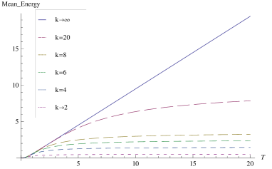
This is of course the trace result straightforwardly computed in the canonical basis (5). The corresponding mean energy reads

$$\overline{E}_{1}(\beta)=-\frac{\partial\log{\cal Z}_{1}(\beta)}{\partial\beta}=\left(\frac{1}{e^{\beta\epsilon}-1}-\frac{k}{e^{k\beta\epsilon}-1}\right)\epsilon$$ (54)

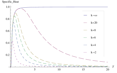
and the specific heat

$$C(\beta)=-\beta^{2}\frac{\partial\overline{E}_{1}}{\partial\beta}=\frac{1}{4}\left(\beta\epsilon\right)^{2}\left(\frac{1}{\sinh^{2}\left(\beta\epsilon/2\right)}-\frac{k^{2}}{\sinh^{2}\left(k\beta\epsilon/2\right)}\right).$$ (55)

We show in Figures (1, 2) these functions for low values of $k$ together with the limit case $k\to\infty$, to make explicit that the $k$-nilpotent behaviour interpolates between fermionic ($k=2)$ and bosonic ($k\to\infty)$ standard results.

Figure 1: (colour on line) Mean energy of a $q$-boson in a thermal bath, for different nilpotency orders $k$ (in arbitrary units). Notice that at finite $k$ the mean energy saturates at high enough temperatures, where each of the energy levels is found with equal probability. In contrast, for standard bosons ($k\to\infty)$ the mean energy grows linearly with temperature.

Figure 2: (colour on line) Specific heat for different nilpotency orders $k$ (in arbitrary units). Notice that at finite $k$ the specific heat has a maximum and decays to zero when the mean energy saturates. For standard bosons this does not occur (no saturation is possible).

A similar analysis can be done for one $q$-boson oscillator with Hamiltonian

$$H_{1}^{\prime}=\epsilon a_{1}^{\dagger}a_{1},$$ (56)

which has spectrum $\epsilon_{n_{1}}=[n_{1}]_{q}\epsilon$, $n_{1}=0,\cdots,k-1$. One obtains

$$(\theta_{1}|e^{-\beta H_{1}^{\prime}}|\theta)=\sum_{n_{1}=0}^{k-1}\frac{\bar{\theta}^{n_{1}}\theta^{n_{1}}}{[n_{1}]!}e^{-\beta\epsilon[n_{1}]_{q}},$$ (57)

so the partition function gives

$${\cal Z}_{1}^{\prime}(\beta)=\sum_{n_{1}=0}^{k-1}e^{-\beta\epsilon[n_{1}]_{q}}.$$ (58)

VI.2 System of $q$-bosons

In setting a multi-particle system of nilpotent $q$-bosons one must take into account that a linear transformation (in particular the Fourier transformation) of $q$-boson annihilation or creation operators does not render modes with the same commutation relations. The same occurs with para-Grassmann variables in our approach (and any other in the literature). We restrict to Hamiltonians in which different degrees of freedom do not interact. Speculatively, one can think of a system with a finite dimensional Hilbert space per degree of freedom, such as a spin $S$ system in the presence of strong interactions, which after a suitable transformation leads to independent $k$-nilpotent $q$-boson modes.

Let us consider a system of $m$ $q$-bosons $a_{j}$, $a_{j}^{\dagger}$ with Hamiltonian

$$H=\sum_{j=1}^{m}\epsilon_{j}N_{j}.$$ (59)

The grand partition function at finite temperature $k_{B}T=1/\beta$ is given by

$${\cal Z}(\beta)=Tr\left(e^{-\beta(H-\mu N)}\right),$$ (60)

where $N=\sum_{j=1}^{m}N_{j}$ is the total number operator. One needs to compute

$$(\theta|e^{-\beta(H-\mu N)}|\theta)=(\theta|\prod_{j=1}^{m}e^{-\beta(\epsilon_{j}-\mu)N_{j}}|\theta)$$ (61)

which simply factorizes to give

$$\prod_{j=1}^{m}(\theta_{j}|e^{-\beta(\epsilon_{j}-\mu)N_{j}}|\theta_{j})=\sum_{\{n\}}\frac{\bar{\theta}_{1}^{n_{1}}\theta_{1}^{n_{1}}}{[n_{1}]!}e^{-\beta(\epsilon_{1}-\mu)n_{1}}\cdots\frac{\bar{\theta}_{1}^{n_{m}}\theta_{1}^{n_{m}}}{[n_{m}]!}e^{-\beta(\epsilon_{m}-\mu)n_{m}}$$ (62)

The trace is computed according to (49)

$$\int d\theta\,:\mu(\theta,\bar{\theta})\prod_{j=1}^{m}(\theta_{j}|e^{-\beta(\epsilon_{j}-\mu)N_{j}}|\theta_{j}):\>d\bar{\theta}=\prod_{j=1}^{m}\left(\int d\theta_{j}\,:\mu_{j}(\theta_{j},\bar{\theta}_{j})\sum_{n_{j}}\frac{\bar{\theta}_{j}^{n_{j}}\theta_{j}^{n_{j}}}{[n_{j}]!}e^{-\beta(\epsilon_{j}-\mu)n_{j}}:\>d\bar{\theta}_{j}\right)$$ (63)

giving rise to

$${\cal Z}(\beta)=\prod_{j=1}^{m}\frac{1-e^{-k\beta(\epsilon_{j}-\mu)}}{1-e^{-\beta(\epsilon_{j}-\mu)}}.$$ (64)

The relevant quantity to compute here is the mean occupation number of levels $\epsilon_{j}$, which reads

$$n_{j}(\beta,\mu)=\frac{1}{e^{\beta(\epsilon_{j}-\mu)}-1}-\frac{k}{e^{k\beta(\epsilon_{j}-\mu)}-1}.$$ (65)

For finite $k$ this is well defined even for $\epsilon_{j}=\mu$ (evitable singularity), while the limit $k\to\infty$ is finite only for $\epsilon_{j}>\mu$ (the correct behaviour for standard bosons). In Figure (3), it can be seen that the mean occupation at $\epsilon_{j}=\mu$ is $(k-1)/2$ (identical to fermions, for $k=2$) and diverges for $k\to\infty$ (Bose-Einstein condensation). For $k=3$ the present result for $n(\epsilon)$ is markedly close to the distribution of $\mathbb{Z}_{3}$ parafermions and of particles with $g=1/3$ Haldane exclusion statistics illustrated in Schoutens_1997 .

Figure 3: (colour on line) Average occupation number of levels $\epsilon_{j}$ for a system of $q$-bosons at low temperature. For $k=2$ the behaviour corresponds to fermions, while for $k\to\infty$ it corresponds to standard bosons.

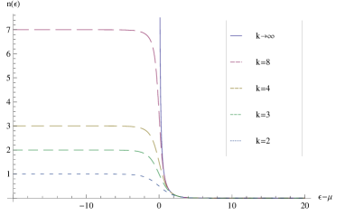
We note again that the $k$-nilpotent behaviour interpolates between fermionic and bosonic standard results.

VII Conclusions

The construction of coherent states for $q$-commuting particles requires the introduction of para-Grassmann variables. In particular, when $q$ is a complex rational primitive root of unity, $q=e^{i\pi/k}$, the required para-Grassmann variables are $k$-nilpotent. Many attempts have been done towards a consistent formulation of nilpotent para-Grassmann calculus, leading to different difficulties in the multiparticle case. In consequence, no consensus has been reached yet in the proper characterization of such nilpotent variables.

We have traced back the source of difficulties, as well as figured forward the applicability, of para-Grassmann variables in systems of nilpotent $q$-bosons. In this work we present a construction, in line with recent proposals El_Baz_2010 ; Sontz_2012 , that incorporates on the one hand para-Grassmann commutation rules which are independent from the nilpotency order, and on the other hand a normal order prescription for the generalized Berezin integration.

Our approach solves the conjugation problem for complex para-Grassmann variables and allows for a consistent symbolic para-Grassmann calculus. In particular it makes possible to handle in much the standard way a resolution of unity as a generalized Berezin integral of multi-particle coherent state projectors. This allows for simple trace formulae, which have been used here to study the thermodynamics of simple Hamiltonians; the distribution of $k$-nilpotent $q$-bosons in a multiparticle system turns out Fermi-like, with mean occupation per mode bounded by $k$. This exclusion statistics could find application in the study of the plethora of novel phases in strongly correlated systems, where different types of ”novel” statistics have already shown up Haldane_PRL67_1991 ; Haldane_PRL66_1991 ; Schoutens_1997 ; Laughlin_1983 ; Palmer_2006 , mainly as a consequence of the strong interactions. In different contexts, constraints in the occupation number of bosons are introduced in order to select a Fock subspace AA ; Buonsante_2008 ; it would be interesting to investigate the connection with our present approach, although it is out of the scope of the present paper. Our formalism allows for a thermodynamical description, hence providing the tools to compare with experimental measurements to come.

Acknowledgements: We thank G. Lozano, N. Grandi and H.D. Rosales for insightful discussions. R.A.R., D.C.C. and G.L.R. are partially supported by CONICET (PIP 1691) and ANPCyT (PICT 1426). E.F.M. is partially supported by NEU, USA.

References

- (1) Gentile G 1940 Nuovo Cimento 17 493
- (2) Leinaas J M and Myrheim J 1977 Nuovo Cimento 37B 1; Wilczek F 1982 Phys. Rev. Lett. 49 957
- (3) Haldane F D M 1991 Phys. Rev. Lett. 67 937
- (4) Green H S 1953 Physical Review 90 270
- (5) Biedenharn L 1989 J. Phys. A: Math. Gen. 22 L873; Macfarlane A J 1989 J. Phys. A: Math. Gen. 22 4581
- (6) Rausch de Traubenberg M and Fleury N 1988 Beyond spinors, in Leite Lopes Festschrift Editors Fleury N et al. (Singapore: World Scientific)
- (7) Filippov A T and Kurdikov A B 1993 arXiv preprint hep-th/9312081
- (8) Baulieu L and Floratos E 1991 Phys. Lett. B 258 171
- (9) Filippov A T, Isaev A P and Kurdikov A B 1992 Mod. Phys. Lett. A 7 2129 ; Filippov A T, Isaev A P and Kurdikov A B 1993 Theor. Math. Phys. 94 150
- (10) Rausch de Traubenberg M 1997 Habilitation Thesis, Université Louis Pasteur; arXiv preprint hep-th/9802141 (in French)
- (11) Cugliandolo L, Lozano G S, Moreno E F and Schaposnik F A 2004 Int. J. Mod. Phys. A 19 1705
- (12) Cabra D C, Moreno E F and Tanasa A 2006 SIGMA 2 087
- (13) El Baz M, Fresneda R, Gazeau J P and Hassouni Y 2010) J. Phys. A: Math. Theor. 43 385202; Erratum (2011).
- (14) Sontz S B 2012 arXiv:1204.1033 .
- (15) Auerbach A and Arovas D 1988 Phys. Rev. Lett. 61 617
- (16) Haldane F D M 1991 Phys. Rev. Lett. 66 1529
- (17) Schoutens K 1994 Phys. Lett. B 331 335
- (18) Halperin B I 1984 Phys. Rev. Lett. 52 1583; Halperin B I 1984 Phys. Rev. Lett. 52 2390(E)
- (19) Schoutens K 1997 Phys. Rev. Lett. 79 2608
- (20) Greenberg O W 1990 Bull. Am. Phys. Soc. 35 981; Greenberg O W 1991 Physical Review D 43 4111
- (21) Parthasarathy R and Viswanathan K S 1991 J. Phys. A: Math. Gen. 24 613; Beckers J, Debergh N 1991 J. Phys. A: Math. Gen. 24 L1277
- (22) Chaichian M, Gonzalez Felipe R and Montonen C 1993 J. Phys. A: Math. Gen. 26 4017
- (23) Avancini S S, Marinelli J R and Krein G 2003 J. Phys. A: Math. Theor. 36 9045
- (24) Mirza B and Mohammadzadeh H 2011 J. Phys. A: Math. Theor. 44 475003
- (25) Gavrilik A M, Kachurik I I and Mishchenko Y A 2011 J. Phys. A: Math. Theor. 44 475303
- (26) Shabanov S 1993 J. Phys. A: Math. Gen. 26 2583
- (27) Floratos E 1991 J. Phys. A: Math. Gen. 24 4739
- (28) Ohnuki Y and Kashiwa T 1978 Prog. Theor. Phys. 60 548
- (29) Majid S and Rodríguez-Plaza M J 1994 J. Math. Phys. 35 3753
- (30) Berezin F 1971 Math. URSS Sbornik 15 577
- (31) Ramirez R A PhD Thesis, in preparation
- (32) Perelomov A 1986 Generalized Coherent States and their applications (Berlin: Springer-Verlag)
- (33) Ramirez R A, Rossini G L and Sanmartino M 2012 IJPAM 76 79
- (34) Laughlin R B 1983 Phys. Rev. Lett. 50 1395
- (35) Palmer R and Jaksch D Phys. Rev. Lett. 96 180407
- (36) Buonsante P and Penna V 2008 J. Phys. A: Math. Theor. 41 175301