SLAC–PUB–15251

The six-point remainder function
to all loop orders in the multi-Regge limit

Jeffrey Pennington
SLAC National Accelerator Laboratory, Stanford University,
Stanford, CA 94309, USA
Email: jpennin@stanford.edu

Abstract

We present an all-orders formula for the six-point amplitude of planar maximally supersymmetric ${\mathcal{N}}=4$ Yang-Mills theory in the leading-logarithmic approximation of multi-Regge kinematics. In the MHV helicity configuration, our results agree with an integral formula of Lipatov and Prygarin through at least 14 loops. A differential equation linking the MHV and NMHV helicity configurations has a natural action in the space of functions relevant to this problem—the single-valued harmonic polylogarithms introduced by Brown. These functions depend on a single complex variable and its conjugate, $w$ and ${w^{\ast}}$, which are quadratically related to the original kinematic variables. We investigate the all-orders formula in the near-collinear limit, which is approached as $|w|\to 0$. Up to power-suppressed terms, the resulting expansion may be organized by powers of $\log|w|$. The leading term of this expansion agrees with the all-orders double-leading-logarithmic approximation of Bartels, Lipatov, and Prygarin. The explicit form for the sub-leading powers of $\log|w|$ is given in terms of modified Bessel functions.

1 Introduction

In recent years, considerable progress has been made in the study of relativistic scattering amplitudes in gauge theory and gravity. A growing set of computational tools, including unitarity [1], BCFW recursion [2, 3, 4, 5], BCJ duality [6, 7], and symbology [8, 9, 10, 11, 12], has facilitated many impressive perturbative calculations at weak coupling. The AdS/CFT correspondence has provided access to the new, previously inaccessible frontier of strong coupling [13]. The theory that has reaped the most benefit from these advances is, arguably, maximally supersymmetric ${\mathcal{N}}=4$ Yang-Mills theory, specifically in the planar limit of a large number of colors. Indeed, ${\mathcal{N}}=4$ super-Yang-Mills theory provides an excellent laboratory for the AdS/CFT correspondence, as well as for the structure of gauge theory amplitudes in general.

One of the reasons for the relative simplicity of ${\mathcal{N}}=4$ super-Yang-Mills theory is its high degree of symmetry. The extended supersymmetry puts strong constraints on the form of scattering amplitudes, and it guarantees a conformal symmetry in position space. Recently, an additional conformal symmetry was found in the planar theory [13, 14, 15, 16, 17, 18, 19]. It acts on a set of dual variables, $x_{i}$, which are related to the external momenta $k_{i}^{\mu}$ by $k_{i}=x_{i}-x_{i+1}$. At tree level, this dual conformal symmetry can be extended to a dual super-conformal symmetry [20] and even combined with the original conformal symmetry into an infinite-dimensional Yangian symmetry [21]. At loop level, the dual conformal symmetry is broken by infrared divergences. According to the Wilson-loop/amplitude duality [13, 16, 17], these infrared divergences can be understood as ultraviolet divergences of particular polygonal Wilson loops. In this context, the breaking of dual conformal symmetry is governed by an anomalous Ward identity [19, 22]. For maximally-helicity violating (MHV) amplitudes, a solution to the Ward identity may be written as,

$$A_{n}^{\textrm{MHV}}=A_{n}^{\textrm{BDS}}\times\exp(R_{n}),$$ (1.1)

where $A_{n}^{\textrm{BDS}}$ is an all-loop, all-multiplicity ansatz proposed by Bern, Dixon, and Smirnov [23], and $R_{n}$ is a dual-conformally invariant function referred to as the remainder function [24, 25].

Dual conformal invariance provides a strong constraint on the form of $R_{n}$. For example, it is impossible to construct a non-trivial dual-conformally invariant function with fewer than six external momenta. As a result, $R_{4}=R_{5}=0$, and, consequently, the four- and five-point scattering amplitudes are equal to the BDS ansatz. At six points, there are three independent invariant cross ratios built from distances $x_{ij}^{2}$ in the dual space,

$$u_{1}=\frac{x_{13}^{2}x_{46}^{2}}{x_{14}^{2}x_{36}^{2}}=\frac{s_{12}s_{45}}{s_{123}s_{345}}\,,\qquad u_{2}=\frac{x_{24}^{2}x_{15}^{2}}{x_{25}^{2}x_{14}^{2}}=\frac{s_{23}s_{56}}{s_{234}s_{456}}\,,\qquad u_{3}=\frac{x_{35}^{2}x_{26}^{2}}{x_{36}^{2}x_{25}^{2}}=\frac{s_{34}s_{61}}{s_{345}s_{561}}\,.$$ (1.2)

Dual conformal invariance restricts $R_{6}$ to be a function of these variables only, i.e. $R_{6}=R_{6}(u_{1},u_{2},u_{3})$. This function is not arbitrary since, among other conditions, it must be totally symmetric under permutations of the $u_{i}$ and vanish in the collinear limit [24].

In the absence of an explicit computation, it remained a possibility that $R_{6}=0$, despite the fact that all known symmetries allow for a non-zero function $R_{6}(u_{1},u_{2},u_{3})$. However, a series of calculations have since been performed and they showed definitively that $R_{6}\neq 0$. The first evidence of a non-vanishing $R_{6}$ came from an analysis of the multi-Regge limits of $2\to 4$ gluon scattering amplitudes at two loops [26]. Numerical evidence was soon found at specific kinematic points [24, 25], and an explicit calculation for general kinematics followed shortly thereafter [27, 28]. Interestingly, the two-loop calculation for general kinematics was actually performed in a quasi-multi-Regge limit; the full kinematic dependence could then be inferred because this type of Regge limit does not modify the analytic dependence of the remainder function on the $u_{i}$.

Even beyond the two-loop remainder function, the limit of multi-Regge kinematics (MRK) has received considerable attention in the context of ${\mathcal{N}}=4$ super-Yang Mills theory [26, 29, 30, 31, 32, 33, 34, 35, 36, 37, 38, 39, 40, 41]. One reason for this is that multi-leg scattering amplitudes become considerably simpler in MRK while still maintaining a non-trivial analytic structure. Taking the multi-Regge limit at six points, for example, essentially reduces the amplitude to a function of just two variables, $w$ and ${w^{\ast}}$, which are complex conjugates of each other. This latter point has proved particularly important in describing the relevant function space in this limit. In fact, it has been argued recently [40] that the function space is spanned by the set of single-valued harmonic polylogarithms (SVHPLs) introduced by Brown [42]. These functions will play a prominent role in the remainder of this article.

The MRK limit of $2\to 4$ scattering is characterized by the condition that the outgoing particles are widely separated in rapidity while having comparable transverse momenta. In terms of the cross ratios $u_{i}$, the limit is approached by sending one of the $u_{i}$, say $u_{1}$, to unity, while letting the other two cross ratios vanish at the same rate that $u_{1}\to 1$, i.e. $u_{2}=x(1-u_{1})$ and $u_{3}=y(1-u_{1})$ for two fixed variables $x$ and $y$. Actually, this prescription produces the Euclidean version of the MRK limit in which the six-point remainder function vanishes [43, 44, 45]. To reach the Minkowski version, which is relevant for $2\to 4$ scattering, $u_{1}$ must be analytically continued around the origin, $u_{1}\to e^{-2\pi i}|u_{1}|$, before taking the limit. The remainder function may then be expanded around $u_{1}=1$ and the coefficients of this expansion are functions of only two variables, $x$ and $y$. The variables $w$ and ${w^{\ast}}$ mentioned previously are related to $x$ and $y$ by [33, 34],

$$x\equiv{1\over(1+w)(1+{w^{\ast}})},\qquad y\equiv{w\,{w^{\ast}}\over(1+w)(1+{w^{\ast}})}\,.$$ (1.3)

Neglecting terms that vanish like powers of $1-u_{1}$, the expansion of the remainder function may be written as,

$$R_{6}^{\textrm{MHV}}|_{\textrm{MRK}}\,=\,2\pi i\,\sum_{\ell=2}^{\infty}\sum_{n=0}^{\ell-1}a^{\ell}\,\log^{n}(1-u_{1})\,\left[g_{n}^{(\ell)}(w,{w^{\ast}})+2\pi i\,h_{n}^{(\ell)}(w,{w^{\ast}})\right]\,,$$ (1.4)

where the coupling constant for planar ${\mathcal{N}}=4$ super-Yang-Mills theory is $a=g^{2}N_{c}/(8\pi^{2})$. This expansion is organized hierarchically into the leading-logarithmic approximation (LLA) with $n=\ell-1$, the next-to-leading-logarithmic approximation (NLLA) with $n=\ell-2$, and in general the N^kLL terms with $n=\ell-k-1$. In this article, we study the leading-logarithmic approximation, for which we may rewrite eq. (1.4) as,

$$R_{6}^{\textrm{MHV}}|_{\textrm{LLA}}\,=\,\frac{2\pi i}{\log(1-u_{1})}\,\sum_{\ell=2}^{\infty}\eta^{\ell}\,g_{\ell-1}^{(\ell)}(w,{w^{\ast}})\,,$$ (1.5)

where we have identified $\eta=a\log(1-u_{1})$ as the relevant expansion parameter. In LLA, the real part of $R_{6}$ vanishes, so $h_{\ell-1}^{\ell}(w,{w^{\ast}})$ is absent in eq. (1.5). Expressions for $g_{\ell-1}^{(\ell)}(w,{w^{\ast}})$ have been given in the literature for two, three [33], and recently up to ten [40] loops.

An all-orders integral-sum representation for $R_{6}^{\textrm{MHV}}|_{\textrm{LLA}}$ was presented in ref. [33] and was generalized to the NMHV helicity configuration in ref. [39]. (The MHV case was extended to NLLA in ref. [36].) The formula may be understood as an inverse Fourier-Mellin transform from a space of moments labeled by $(\nu,n)$ to the space of kinematic variables $(w,{w^{\ast}})$. In the moment space, $R_{6}|_{\textrm{LLA}}(\nu,n)$ assumes a simple factorized form and may be written succinctly to all loop orders in terms of polygamma functions. This structure is obscured in $(w,{w^{\ast}})$ space, as the inverse Fourier-Mellin transform generates complicated combinations of polylogarithmic functions. Nevertheless, these complicated expressions should bear the mark of their simple ancestry. In this article, we expose this inherited structure by presenting an explicit all-orders formula for $R_{6}|_{\textrm{LLA}}$ directly in $(w,{w^{\ast}})$ space.

We do not present a proof of this formula, but we do test its validity using several non-trivial consistency checks. For example, our result agrees with the integral formula mentioned above through at least 14 loops. In ref. [39], Lipatov, Prygarin, and Schnitzer give a simple differential equation linking the MHV and NMHV helicity configurations,

$${w^{\ast}}\frac{\partial}{\partial{w^{\ast}}}R_{6}^{\textrm{MHV}}|_{\textrm{LLA}}=w\frac{\partial}{\partial w}R_{6}^{\textrm{NMHV}}|_{\textrm{LLA}}\,,$$ (1.6)

which is also obeyed our formula. In the near-collinear limit, we find agreement with the all-orders double-leading-logarithmic approximation of Bartels, Lipatov, and Prygarin [46].

This article is organized as follows. In Section 2, we review the aspects of multi-Regge kinematics relevant to six-particle scattering and recall the integral formulas for $R_{6}|_{\textrm{LLA}}$ in the MHV and NMHV helicity configurations. The construction and properties of single-valued harmonic polylogarithms are reviewed in Section 3. An all-orders expression for $R_{6}|_{\textrm{LLA}}$ is presented in terms of these functions in Section 4. After verifying several consistency conditions of this formula, we examine its near-collinear limit in Section 5. Section 6 offers some concluding remarks and prospects for future work.

2 The six-point remainder function in multi-Regge kinematics

We consider the six-gluon scattering process $g_{3}g_{6}\to g_{1}g_{5}g_{4}g_{2}$ where the momenta are taken to be outgoing and the gluons are labeled cyclically in the clockwise direction. The limit of multi-Regge kinematics is defined by the condition that the produced gluons are strongly ordered in rapidity while having comparable transverse momenta,

$$y_{1}\gg y_{5}\gg y_{4}\gg y_{2}\,,\quad\quad|p_{1\perp}|\simeq|p_{5\perp}|\simeq|p_{4\perp}|\simeq|p_{2\perp}|\,.$$ (2.1)

In the Euclidean region, this limit is equivalent to the hierarchy of scales,

$$s_{12}\gg s_{345},\,s_{456}\gg s_{34},\,s_{45}\,,s_{56}\gg s_{23},\,s_{61},\,s_{234},$$ (2.2)

which leads to the limiting behavior of the cross ratios (1.2),

$$1-u_{1},\,u_{2},\,u_{3}\sim 0\,,$$ (2.3)

subject to the constraint that the following ratios are held fixed,

$$x\equiv{u_{2}\over 1-u_{1}}={\mathcal{O}}(1){\rm~{}~{}and~{}~{}}y\equiv{u_{3}\over 1-u_{1}}={\mathcal{O}}(1)\,.$$ (2.4)

Unitarity restricts the branch cuts of physical quantities like the remainder function $R_{6}(u_{1},u_{2},u_{3})$ to appear in physical channels. In terms of the cross ratios $u_{i}$, this requirement implies that all branch points occur when a cross ratio vanishes or approaches infinity. If we re-express the two real variables $x$ and $y$ by a single complex variable $w$,

$$x\equiv{1\over(1+w)(1+{w^{\ast}})}{\rm~{}~{}and~{}~{}}y\equiv{w\,{w^{\ast}}\over(1+w)(1+{w^{\ast}})}\,,$$ (2.5)

then the equivalent statement in MRK is that any function of $(w,{w^{\ast}})$ must be single-valued in the complex $w$ plane.

In the Euclidean region, the remainder function actually vanishes in the multi-Regge limit. To obtain a non-vanishing result, we must consider a physical region in which one of the cross ratios acquires a phase [26]. One such region corresponds to the $2\to 4$ scattering process described above. It can be reached by flipping the signs of $s_{12}$ and $s_{45}$, or, in terms of the cross ratios, by rotating $u_{1}$ around the origin,

$$u_{1}\to e^{-2\pi i}\,|u_{1}|\,.$$ (2.6)

In the course of this analytic continuation, we pick up the discontinuity across a Mandelstam cut [26, 31]. The six-point remainder function can then be expanded in the form given in eq. (1.4),

$$R_{6}^{\textrm{MHV}}|_{\textrm{MRK}}=2\pi i\,\sum_{\ell=2}^{\infty}\sum_{n=0}^{\ell-1}a^{\ell}\,\log^{n}(1-u_{1})\,\left[g_{n}^{(\ell)}(w,{w^{\ast}})+2\pi i\,h_{n}^{(\ell)}(w,{w^{\ast}})\right]\,.$$ (2.7)

The large logarithms $\log(1-u_{1})$ organize this expansion into the leading-logarithmic approximation (LLA) with $n=\ell-1$, the next-to-leading-logarithmic approximation (NLLA) with $n=\ell-2$, and in general the the N^kLL terms with $n=\ell-k-1$.

In refs. [33, 36] an all-loop integral formula for $R_{6}^{\textrm{MHV}}|_{\textrm{MRK}}$ was presented for LLA and NLLA,

$$e^{R+i\pi\delta}|_{\textrm{MRK}}=\cos\pi\omega_{ab}+i\,{a\over 2}\sum_{n=-\infty}^{\infty}(-1)^{n}\,\left({w\over{w^{\ast}}}\right)^{{n\over 2}}\int_{-\infty}^{+\infty}{d\nu\over\nu^{2}+{n^{2}\over 4}}\,|w|^{2i\nu}\,\Phi_{\textrm{Reg}}(\nu,n)\,\left(-{1\over\sqrt{u_{2}\,u_{3}}}\right)^{\omega(\nu,n)}.$$ (2.8)

Here, $\omega(\nu,n)$ is the BFKL eigenvalue and $\Phi_{\textrm{Reg}}(\nu,n)$ is the regularized impact factor. They may be expanded perturbatively,

$$\begin{split}\omega(\nu,n)&\,=-a\left(E_{\nu,n}+a\,E_{\nu,n}^{(1)}+a^{2}\,E_{\nu,n}^{(2)}+{\mathcal{O}}(a^{3})\right)\,,\\ \Phi_{\textrm{Reg}}(\nu,n)&\,=1+a\,\Phi_{\textrm{Reg}}^{(1)}(\nu,n)+a^{2}\,\Phi_{\textrm{Reg}}^{(2)}(\nu,n)+a^{3}\,\Phi_{\textrm{Reg}}^{(3)}(\nu,n)+{\mathcal{O}}(a^{4})\,.\end{split}$$ (2.9)

The leading-order eigenvalue, $E_{\nu,n}$, was given in ref. [29] and may be written in terms of the digamma function $\psi(z)={d\over dz}\log\Gamma(z)$,

$$E_{\nu,n}=-{1\over 2}\,{|n|\over\nu^{2}+{n^{2}\over 4}}+\psi\left(1+i\nu+{|n|\over 2}\right)+\psi\left(1-i\nu+{|n|\over 2}\right)-2\psi(1)\,.$$ (2.10)

In this article, we will only need the leading-order terms, but, remarkably, the higher-order corrections listed in (2.9) may also be expressed in terms of the $\psi$ function and its derivatives [36, 40].

Returning to (2.8), the remaining functions are,

$$\begin{split}\omega_{ab}&\;=\;{1\over 8}\,\gamma_{K}(a)\,\log{u_{3}\over u_{2}}={1\over 8}\,\gamma_{K}(a)\,\log|w|^{2}\,,\\ \delta&\;=\;{1\over 8}\,\gamma_{K}(a)\,\log{(xy)}={1\over 8}\,\gamma_{K}(a)\,\log{|w|^{2}\over|1+w|^{4}}\,,\end{split}$$ (2.11)

and the cusp anomalous dimension, which is known to all orders in perturbation theory [47],

$$\gamma_{K}(a)\,=\,\sum_{\ell=1}^{\infty}\gamma_{K}^{(\ell)}a^{\ell}\,=\,4\,a-4\,\zeta_{2}\,a^{2}+22\,\zeta_{4}\,a^{3}-(\textstyle{\frac{219}{2}}\,\zeta_{6}+4\,\zeta_{3}^{2})\,a^{4}+\cdots\,.$$ (2.12)

In addition, there is an ambiguity regarding the Riemann sheet of the exponential factor on the right-hand side of (2.8). We resolve this ambiguity with the identification,

$$\left(-{1\over\sqrt{u_{2}\,u_{3}}}\right)^{\omega(\nu,n)}\to e^{-i\pi\omega(\nu,n)}\,\left({1\over 1-u_{1}}\,{|1+w|^{2}\over|w|}\right)^{\omega(\nu,n)}\,.$$ (2.13)

The $i\pi$ factor in the right-hand side of eq. (2.13) generates the real parts $h_{n}^{(\ell)}$ in eq. (2.7). For example, at LLA and NLLA, the following relations [40] are satisfied,

$$\begin{split}h_{\ell-1}^{(\ell)}(w,{w^{\ast}})&\,=0\,,\\ h_{\ell-2}^{(\ell)}(w,{w^{\ast}})&\,={\ell-1\over 2}\,g_{\ell-1}^{(\ell)}(w,{w^{\ast}})+{1\over 16}\,\gamma_{K}^{(1)}\,g_{\ell-2}^{(\ell-1)}(w,{w^{\ast}})\,\log{|1+w|^{4}\over|w|^{2}}\\ &\quad-\frac{1}{2}\sum_{k=2}^{\ell-2}g_{k-1}^{(k)}g_{\ell-k-1}^{(\ell-k)}\,,\qquad\ell>2,\end{split}$$ (2.14)

where $\gamma_{K}^{(1)}=4$ from eq. (2.12). Making use of eq. (1.5), we present an alternate form of these identities which will be useful later,

$$\begin{split}\textrm{Re}\left(R_{6}^{\textrm{MHV}}|_{\textrm{NLLA}}\right)&\;=\;\frac{2\pi i}{\log(1-u_{1})}\bigg{(}\frac{1}{2}\,\eta^{2}\,\frac{\partial}{\partial\eta}\,\frac{1}{\eta}+\frac{\gamma_{K}^{(1)}}{16}\,\eta\,\log\frac{|1+w|^{4}}{|w|^{2}}\,\bigg{)}\,R_{6}^{\textrm{MHV}}|_{\textrm{LLA}}\\ &\quad+\frac{2\pi^{2}}{\log^{2}(1-u_{1})}\eta^{2}g^{(2)}_{1}(w,{w^{\ast}})-\frac{1}{2}\left(R_{6}^{\textrm{MHV}}|_{\textrm{LLA}}\right)^{2}\,.\end{split}$$ (2.15)

The term proportional to $g^{(2)}_{1}(w,{w^{\ast}})$ addresses the special case of $\ell=2$ in eq. (2.14).

In what follows, we will focus on the leading-logarithmic approximation of (2.8), which takes the form,

$$R_{6}^{\textrm{MHV}}|_{\textrm{LLA}}=i{a\over 2}\sum_{n=-\infty}^{\infty}(-1)^{n}\,\int_{-\infty}^{+\infty}{d\nu\,w^{i\nu+n/2}\,{w^{\ast}}^{i\nu-n/2}\over(i\nu+{n\over 2})(-i\nu+{n\over 2})}\,\bigg{[}(1-u_{1})^{a\,E_{\nu,n}}-1\bigg{]}\,.$$ (2.16)

The $\nu$-integral may be evaluated by closing the contour and summing residues. To perform the resulting double sums, one may apply the summation algorithms of ref. [48], although this approach is computationally challenging for high loop orders. Alternatively, an ansatz for the result may be expanded around $|w|=0$ and matched term-by-term to the truncated double sum. The latter method requires knowledge of the complete set of functions that might arise in this context. In ref. [40], it was argued that the single-valued harmonic polylogarithms (SVHPLs) completely characterize this function space, and, using these functions, eq. (2.16) was evaluated through ten loops.

So far we have only discussed the MHV helicity configuration. We now turn to the only other independent helicity configuration at six points, the NMHV configuration. In MRK, the MHV and NMHV tree amplitudes are equal [49, 39]. It is natural, therefore, to define an NMHV remainder function, analogous to eq. (1.1),

$$A_{6}^{\textrm{NMHV}}|_{\textrm{MRK}}=A_{6}^{\textrm{BDS}}\times\exp(R_{\textrm{NMHV}})\,.$$ (2.17)

In ref. [39], it was argued that the effect of changing the helicity of one of the positive-helicity gluons was equivalent to changing the impact factor for that gluon by means of the following replacement,

$${1\over-i\nu+{n\over 2}}\to-{1\over i\nu+{n\over 2}}\,.$$ (2.18)

Referring to eq. (2.16), this replacement leads to an integral formula for $R_{6}^{\textrm{NMHV}}|_{\textrm{LLA}}$,

$$R_{6}^{\textrm{NMHV}}|_{\textrm{LLA}}=-{ia\over 2}\,\sum_{n=-\infty}^{\infty}(-1)^{n}\,\int_{-\infty}^{+\infty}{d\nu\,w^{i\nu+n/2}\,{w^{\ast}}^{i\nu-n/2}\over(i\nu+{n\over 2})^{2}}\,\bigg{[}(1-u_{1})^{a\,E_{\nu,n}}-1\bigg{]}\,.$$ (2.19)

Following refs. [39] and [40], we can extract a simple rational prefactor and write eq. (2.19) in a manifestly inversion-symmetric form,

$$R_{6}^{\textrm{NMHV}}|_{\textrm{LLA}}=\frac{2\pi i}{\log(1-u_{1})}\,\sum_{\ell=2}^{\infty}\frac{\eta^{\ell}}{1+{w^{\ast}}}f^{(\ell)}(w,{w^{\ast}})\;+\;\bigg{\{}(w,{w^{\ast}})\leftrightarrow\left(\frac{1}{w},\frac{1}{{w^{\ast}}}\right)\bigg{\}}\,,$$ (2.20)

for some single-valued functions $f^{(\ell)}(w,{w^{\ast}})$. It is possible to obtain expressions for $f^{(\ell)}(w,{w^{\ast}})$ directly from eq. (2.19) by means of the truncated series approach outlined above, for example. A simpler method is to make use of the following differential equation, which may be deduced by comparing the two expressions (2.16) and (2.19),

$${w^{\ast}}\frac{\partial}{\partial{w^{\ast}}}R_{6}^{\textrm{MHV}}|_{\textrm{LLA}}=w\frac{\partial}{\partial w}R_{6}^{\textrm{NMHV}}|_{\textrm{LLA}}\,.$$ (2.21)

In principle, solving this equation requires the difficult step of fixing the constants of integration in such a way that single-valuedness is preserved. As discussed in ref. [40], this step becomes trivial when working in the space of SVHPLs, which are the subject of the next section.

3 Review of single-valued harmonic polylogarithms

Harmonic polylogarithms (HPLs) [50] are a class of generalized polylogarithmic functions that finds frequent application in multi-loop calculations. The HPLs are functions of a single complex variable, $z$, which will be related to the kinematic variable $w$ by $z=-w$. We will continue to use $z$ throughout this section in order to make contact with the existing mathematical literature. In general, the HPLs have branch cuts that originate at $z=-1$, $z=0$, or $z=1$. In the present application, we will consider the restricted class of HPLs whose branch points are either $z=0$ or $z=1$. To construct them, consider the set $X^{*}$ of all words $w$ formed from the letters $x_{0}$ and $x_{1}$, together with $e$, the empty word. Then, for each $w\in X^{*}$, define a function $H_{w}(z)$ which obeys the differential equations,

$$\frac{\partial}{\partial z}H_{x_{0}w}(z)=\frac{H_{w}(z)}{z}\quad\quad\text{and}\quad\quad\frac{\partial}{\partial z}H_{x_{1}w}(z)=\frac{H_{w}(z)}{1-z}\,,$$ (3.1)

subject to the following conditions,

$$H_{e}(z)=1,\quad\quad H_{x_{0}^{n}}(z)=\frac{1}{n!}\log^{n}z,\quad\quad\text{and}\quad\quad\lim_{z\rightarrow 0}H_{w\neq x_{0}^{n}}(z)=0\,.$$ (3.2)

There is a unique family of solutions to these equations, and it defines the HPLs. For $w\neq x_{0}^{n}$, they can be written as iterated integrals,

$$H_{x_{0}w}(z)=\int_{0}^{z}dz^{\prime}\;\frac{H_{w}(z^{\prime})}{z^{\prime}}\quad\quad\text{and}\quad\quad H_{x_{1}w}=\int_{0}^{z}dz^{\prime}\;\frac{H_{w}(z^{\prime})}{1-z^{\prime}}\,.$$ (3.3)

The structure of the iterated integrals endows the HPLs with an important property: they form a shuffle algebra. The shuffle relations can be written as,

$$H_{w_{1}}(z)\,H_{w_{2}}(z)=\sum_{{w}\in{w_{1}}\mbox{\bf\scyr X}{w_{2}}}H_{w}(z)\,,$$ (3.4)

where ${w_{1}}{\mbox{\cyr X}}{w_{2}}$ is the set of mergers of the sequences $w_{1}$ and $w_{2}$ that preserve their relative ordering. The shuffle algebra may be used to remove all zeros from the right of an index vector in favor of some explicit logarithms. For example, it is easy to obtain the following formula for HPLs with a single $x_{1}$,

$$H_{x_{0}^{n}x_{1}x_{0}^{m}}=\sum_{j=0}^{m}\frac{(-1)^{j}}{(m-j)!}\binom{n+j}{j}H_{x_{0}}^{m-j}H_{x_{0}^{n+j}x_{1}}\,.$$ (3.5)

After removing all right-most zeros, the Taylor expansions around $z=0$ are particularly simple and involve only a special class of harmonic numbers [50],

$$H_{m_{1},\ldots,m_{k}}(z)=\sum_{l=1}^{\infty}{z^{l}\over l^{m_{1}}}Z_{m_{2},\ldots,m_{k}}(l-1)\,,\qquad m_{i}>0\,,$$ (3.6)

where $Z_{m_{1},\ldots,m_{k}}(n)$ are Euler-Zagier sums [51, 52], defined recursively by

$$Z(n)=1{\rm~{}~{}and~{}~{}}Z_{m_{1},\ldots,m_{k}}(n)=\sum_{l=1}^{n}{1\over l^{m_{1}}}Z_{m_{2},\ldots,m_{k}}(l-1)\,.$$ (3.7)

Note that the indexing of the weight vectors $m_{1},\ldots,m_{k}$ in eqs. (3.6) and (3.7) is in the collapsed notation in which a subscript $m$ denotes $m-1$ zeros followed by a single $1$.

The HPLs are multi-valued functions; nevertheless, it is possible to build specific combinations such that the branch cuts cancel and the result is single-valued. An algorithm that explicitly constructs these combinations was presented in ref. [42] and reviewed in ref. [40]. Here we provide a very brief description.

The SVHPLs ${\mathcal{L}}_{w}(z)$ are generated by the series,

$${\mathcal{L}}(z)=L_{X}(z)\tilde{L}_{Y}(\bar{z})\equiv\sum_{w\in X^{*}}{\mathcal{L}}_{w}(z)w\,,$$ (3.8)

where,

$$L_{X}(z)\,=\,\sum_{w\in X^{*}}H_{w}(z)w\,,\qquad\tilde{L}_{Y}(\bar{z})\,=\,\sum_{w\in Y^{*}}H_{\phi(w)}(\bar{z})\tilde{w}\,.$$ (3.9)

Here ${}^{\sim}:X^{*}\rightarrow X^{*}$ is the operation that reverses words, $\phi:Y^{*}\rightarrow X^{*}$ is the map that renames $y$ to $x$, and $Y^{*}$ is the set of words in $\{y_{0},y_{1}\}$, which are defined by the relations,

$$\begin{split}y_{0}&\,=\,x_{0}\\ \tilde{Z}(y_{0},y_{1})y_{1}\tilde{Z}(y_{0},y_{1})^{-1}&\,=\,Z(x_{0},x_{1})^{-1}x_{1}Z(x_{0},x_{1}),\end{split}$$ (3.10)

where $Z(x_{0},x_{1})$ is a generating function of multiple zeta values,

$$Z(x_{0},x_{1})=\sum_{w\in X^{*}}\zeta(w)w.$$ (3.11)

The $\zeta(w)$ are regularized by the shuffle algebra and obey $\zeta(w\neq x_{1})=H_{w}(1)$ and $\zeta(x_{1})=0$.

Alternatively, one may formally define these functions as solutions to simple differential equations, i.e. the ${\mathcal{L}}_{w}(z)$ are the unique single-valued linear combinations of functions $H_{w_{1}}(z)H_{w_{2}}(\bar{z})$ that obey the differential equations [42],

$$\frac{\partial}{\partial z}{\mathcal{L}}_{x_{0}w}(z)=\frac{{\mathcal{L}}_{w}(z)}{z}\quad\quad\text{and}\quad\quad\frac{\partial}{\partial z}{\mathcal{L}}_{x_{1}w}(z)=\frac{{\mathcal{L}}_{w}(z)}{1-z}\,,$$ (3.12)

subject to the conditions,

$${\mathcal{L}}_{e}(z)=1\,,\quad\quad{\mathcal{L}}_{x_{0}^{n}}(z)=\frac{1}{n!}\log^{n}|z|^{2}\quad\quad\text{and}\quad\quad\lim_{z\rightarrow 0}{\mathcal{L}}_{w\neq x_{0}^{n}}(z)=0\,.$$ (3.13)

The SVHPLs also obey differential equations in $\bar{z}$. Both sets of equations are represented nicely in terms of the generating function (3.8),

$$\frac{\partial}{\partial z}{\mathcal{L}}(z)=\left(\frac{x_{0}}{z}+\frac{x_{1}}{1-z}\right){\mathcal{L}}(z)\quad\quad\textrm{and}\quad\quad\frac{\partial}{\partial\bar{z}}{\mathcal{L}}(z)={\mathcal{L}}(z)\left(\frac{y_{0}}{\bar{z}}+\frac{y_{1}}{1-\bar{z}}\right).$$ (3.14)

4 Six-point remainder function in MRK and LLA

The SVHPLs introduced in the previous section provide a convenient basis of functions to describe the six-point remainder function in MRK. In ref. [40], these functions were used to express the result through ten loops in LLA and through nine loops in NLLA. Here we use the SVHPLs to present a formula in LLA to all loop orders.

4.1 The all-orders formula

Recall from the previous section that we defined $X^{*}$ to be the set of all words $w$ in the letters $x_{0}$ and $x_{1}$ together with the empty word $e$. Let $\mathbb{C}\langle X\rangle$ be the complex vector space generated by $X^{*}$ and let $\mathbb{C}\langle{\mathcal{L}}\rangle$ be the complex vector space spanned by the SVHPLs, ${\mathcal{L}}_{w}$ with $w\in X^{*}$. Denote by $\mathbb{C}\langle X\rangle[[\eta]]$ and $\mathbb{C}\langle{\mathcal{L}}\rangle[[\eta]]$ the rings of formal power series in the variable $\eta=a\log(1-u_{1})$ with coefficients in $\mathbb{C}\langle X\rangle$ and $\mathbb{C}\langle{\mathcal{L}}\rangle$, respectively. There is a natural map, $\rho$, which sends words to the corresponding SVHPLs,

$$\begin{split}\rho:\mathbb{C}\langle X\rangle[[\eta]]&\,\rightarrow\,\mathbb{C}\langle{\mathcal{L}}\rangle[[\eta]]\\ w&\,\mapsto\,{\mathcal{L}}_{w}\,.\end{split}$$ (4.1)

Using these ingredients, we propose the following formulas for the MHV and NMHV remainder functions in MRK and LLA,

$$R_{6}^{\textrm{MHV}}|_{\textrm{LLA}} = \frac{2\pi i}{\log(1-u_{1})}\,\rho\Big{(}\mathcal{X}{\cal Z}^{\textrm{MHV}}-\frac{1}{2}\,x_{1}\eta\Big{)}\,,$$ (4.2)

$$R_{6}^{\textrm{NMHV}}|_{\textrm{LLA}} = \frac{2\pi i}{\log(1-u_{1})}\,\frac{1}{1+{w^{\ast}}}\,\rho\Big{(}x_{0}\mathcal{X}{\cal Z}^{\textrm{NMHV}}\Big{)}\;+\;\bigg{\{}(w,{w^{\ast}})\leftrightarrow\left(\frac{1}{w},\frac{1}{{w^{\ast}}}\right)\bigg{\}}\,,$$ (4.3)

where the formal power series $\mathcal{X},{\cal Z}^{\textrm{(N)MHV}}\in\mathbb{C}\langle X\rangle[[\eta]]$ are,

$$\begin{split}\mathcal{X}&\,=\,e^{\frac{1}{2}x_{0}\eta}\left[1-x_{1}\left(\frac{e^{x_{0}\eta}-1}{x_{0}}\right)\right]^{-1}\,,\\ {\cal Z}^{\textrm{MHV}}&\,=\,\frac{1}{2}\sum_{k=1}^{\infty}\left(x_{1}\,\sum_{n=0}^{k-1}(-1)^{n}x_{0}^{k-n-1}\sum_{m=0}^{n}\,\frac{2^{2m-k+1}}{(k-m-1)!}\,\mathfrak{Z}(n,m)\right)\eta^{k}\,,\\ {\cal Z}^{\textrm{NMHV}}&\,=\,\frac{1}{2}\sum_{k=2}^{\infty}\left(x_{1}\,\sum_{n=0}^{k-2}(-1)^{n}x_{0}^{k-n-2}\sum_{m=0}^{n}\,\frac{2^{2m-k+1}}{(k-m-1)!}\,\mathfrak{Z}(n,m)\right)\eta^{k}\,.\end{split}$$ (4.4)

Here, the $\mathfrak{Z}(n,m)$ are particular combinations of $\zeta$ values of uniform weight $n$. They are related to partial Bell polynomials, and are generated by the series,

$$\exp\left[y\sum_{k=1}^{\infty}\zeta_{2k+1}x^{2k+1}\right]\equiv\sum_{n=0}^{\infty}\sum_{m=0}^{\infty}\mathfrak{Z}(n,m)\,x^{n}y^{m}\,.$$ (4.5)

An explicit formula is,

$$\mathfrak{Z}(n,m)\;\;=\sum_{\beta\in P(n,m)}\prod_{i}\frac{(\zeta_{2i+1})^{\beta_{i}}}{\beta_{i}!}\,,$$ (4.6)

where $P(n,m)$ is the set of $n$-tuples of non-negative integers that sum to $m$, such that the product of $\zeta$ values has weight $n$,

$$P(n,m)\,=\,\left\{\{\beta_{1},\cdots,\beta_{n}\}\,\Big{|}\,\beta_{i}\in\mathbb{N}_{0},\;\sum_{i=1}^{n}\beta_{i}=m,\;\sum_{i=1}^{n}(2i+1)\beta_{i}=n\right\}\,.$$ (4.7)

Similarly, an expression for the $k$th term of $\mathcal{X}$ can be given as,

$$\mathcal{X}=\sum_{k=0}^{\infty}\left(\sum_{n=0}^{k}\frac{x_{0}^{k-n}}{2^{k-n}\,(k-n)!}\sum_{\alpha\in Q(n)}\prod_{j}\frac{x_{1}x_{0}^{\alpha_{j}-1}}{\alpha_{j}!}\right)\eta^{k}\,,$$ (4.8)

where $Q(n)$ is the set of integer compositions of $n$,

$$Q(n)\,=\,\left\{\{\alpha_{1},\alpha_{2},\cdots,\alpha_{m}\}\,\Big{|}\,\alpha_{i}\in\mathbb{Z}^{+},\;\sum_{i=1}^{m}\alpha_{i}=n\right\}\,.$$ (4.9)

Excluding the one-loop term in eq. (4.2), the arguments of the $\rho$ functions factorize into the product of a $\zeta$-free function, $\mathcal{X}$, and a $\zeta$-containing function, ${\cal Z}^{\textrm{(N)MHV}}$. The $\zeta$-free function is simpler and its first few terms read,

$$\begin{split}\mathcal{X}&\;=\;1+\left(\frac{1}{2}\,x_{0}+x_{1}\right)\eta+\left(\frac{1}{8}\,x_{0}^{2}+\frac{1}{2}\,x_{0}x_{1}+\frac{1}{2}\,x_{1}x_{0}+x_{1}^{2}\right)\eta^{2}\\ &\quad+\left(\frac{1}{48}\,x_{0}^{3}+\frac{1}{8}\,x_{0}^{2}x_{1}+\frac{1}{4}\,x_{0}x_{1}x_{0}+\frac{1}{2}\,x_{0}x_{1}^{2}+\frac{1}{6}\,x_{1}x_{0}^{2}+\frac{1}{2}\,x_{1}x_{0}x_{1}+\frac{1}{2}\,x_{1}^{2}x_{0}+x_{1}^{3}\right)\eta^{3}+\cdots\,.\end{split}$$ (4.10)

The $\zeta$-containing functions are slightly more complicated. Their first few terms are,

$$\begin{split}{\cal Z}^{\textrm{MHV}}&\;=\;\frac{1}{2}\,x_{1}\,\eta+\frac{1}{4}\,x_{1}x_{0}\,\eta^{2}+\frac{1}{16}\,x_{1}x_{0}^{2}\,\eta^{3}+\left(\frac{1}{96}\,x_{1}x_{0}^{3}-\frac{1}{8}\,\zeta_{3}\,x_{1}\right)\eta^{4}+\cdots\,,\\ {\cal Z}^{\textrm{NMHV}}&\;=\;\frac{1}{4}\,x_{1}\,\eta^{2}+\frac{1}{16}\,x_{1}x_{0}\,\eta^{3}+\frac{1}{96}\,x_{1}x_{0}^{2}\,\eta^{4}+\left(\frac{1}{768}\,x_{1}x_{0}^{3}-\frac{1}{48}\,\zeta_{3}\,x_{1}\right)\eta^{5}+\cdots\,.\end{split}$$ (4.11)

Using eqs. (4.10) and (4.11), one may easily extract $g^{(\ell)}_{\ell-1}$ for $\ell=1,2,3,4$ (cf. eqs. (1.5) and (4.2)). The one loop term vanishes, $g^{(1)}_{0}=0$, and the other functions read,

$$\begin{split}g^{(2)}_{1}&\;=\;\frac{1}{4}\,{\mathcal{L}}_{0,1}+\frac{1}{4}\,{\mathcal{L}}_{1,0}+\frac{1}{2}\,{\mathcal{L}}_{1,1}\,,\\ g^{(3)}_{2}&\;=\;\frac{1}{16}\,{\mathcal{L}}_{0,0,1}+\frac{1}{8}\,{\mathcal{L}}_{0,1,0}+\frac{1}{4}\,{\mathcal{L}}_{0,1,1}+\frac{1}{16}\,{\mathcal{L}}_{1,0,0}+\frac{1}{4}\,{\mathcal{L}}_{1,0,1}+\frac{1}{4}\,{\mathcal{L}}_{1,1,0}+\frac{1}{2}\,{\mathcal{L}}_{1,1,1}\,,\\ g^{(4)}_{3}&\;=\;\frac{1}{96}\,{\mathcal{L}}_{0,0,0,1}+\frac{1}{32}\,{\mathcal{L}}_{0,0,1,0}+\frac{1}{16}\,{\mathcal{L}}_{0,0,1,1}+\frac{1}{32}\,{\mathcal{L}}_{0,1,0,0}+\frac{1}{8}\,{\mathcal{L}}_{0,1,0,1}+\frac{1}{8}\,{\mathcal{L}}_{0,1,1,0}\\ &\qquad+\frac{1}{4}\,{\mathcal{L}}_{0,1,1,1}+\frac{1}{96}\,{\mathcal{L}}_{1,0,0,0}+\frac{1}{12}\,{\mathcal{L}}_{1,0,0,1}\,+\frac{1}{8}\,{\mathcal{L}}_{1,0,1,0}+\frac{1}{4}\,{\mathcal{L}}_{1,0,1,1}+\frac{1}{16}\,{\mathcal{L}}_{1,1,0,0}\\ &\qquad+\frac{1}{4}\,{\mathcal{L}}_{1,1,0,1}+\frac{1}{4}\,{\mathcal{L}}_{1,1,1,0}+\frac{1}{2}\,{\mathcal{L}}_{1,1,1,1}-\frac{1}{8}\,\zeta_{3}\,{\mathcal{L}}_{1}\,.\end{split}$$ (4.12)

Similarly, one may extract the first few $f^{(\ell)}$ (cf. eqs. (2.20) and (4.3)), finding $f^{(1)}=0$ and,

$$\begin{split}f^{(2)}&\;=\;\frac{1}{4}\,{\mathcal{L}}_{0,1}\,,\\ f^{(3)}&\;=\;\frac{1}{8}\,{\mathcal{L}}_{0,0,1}+\frac{1}{16}\,{\mathcal{L}}_{0,1,0}+\frac{1}{4}\,{\mathcal{L}}_{0,1,1}\,,\\ f^{(4)}&\;=\;\frac{1}{32}\,{\mathcal{L}}_{0,0,0,1}+\frac{1}{32}\,{\mathcal{L}}_{0,0,1,0}+\frac{1}{8}\,{\mathcal{L}}_{0,0,1,1}+\frac{1}{96}\,{\mathcal{L}}_{0,1,0,0}+\frac{1}{8}\,{\mathcal{L}}_{0,1,0,1}+\frac{1}{16}\,{\mathcal{L}}_{0,1,1,0}+\frac{1}{4}\,{\mathcal{L}}_{0,1,1,1}\,,\\ f^{(5)}&\;=\;\frac{1}{192}\,{\mathcal{L}}_{0,0,0,0,1}+\frac{1}{128}\,{\mathcal{L}}_{0,0,0,1,0}+\frac{1}{32}\,{\mathcal{L}}_{0,0,0,1,1}+\frac{1}{192}\,{\mathcal{L}}_{0,0,1,0,0}+\frac{1}{16}\,{\mathcal{L}}_{0,0,1,0,1}\\ &\qquad+\frac{1}{32}\,{\mathcal{L}}_{0,0,1,1,0}+\frac{1}{8}\,{\mathcal{L}}_{0,0,1,1,1}+\frac{1}{768}\,{\mathcal{L}}_{0,1,0,0,0}+\frac{1}{24}\,{\mathcal{L}}_{0,1,0,0,1}+\frac{1}{32}\,{\mathcal{L}}_{0,1,0,1,0}\\ &\qquad+\frac{1}{8}\,{\mathcal{L}}_{0,1,0,1,1}+\frac{1}{96}\,{\mathcal{L}}_{0,1,1,0,0}+\frac{1}{8}\,{\mathcal{L}}_{0,1,1,0,1}+\frac{1}{16}\,{\mathcal{L}}_{0,1,1,1,0}+\frac{1}{4}\,{\mathcal{L}}_{0,1,1,1,1}-\frac{1}{48}\,\zeta_{3}\,{\mathcal{L}}_{0,1}\,.\end{split}$$ (4.13)

We do not offer a proof that eqs. (4.2) and (4.3) are valid to all orders in perturbation theory. One may easily check that their expansions through low loop orders, as determined by eqs. (4.12) and (4.13), match the known results [33, 40]. It is also straightforward to extend the above calculations to ten loops and confirm that the results are in agreement with those of ref. [40]. Moreover, we have verified that the truncated series expansion of eq. (4.2) as $|w|\to 0$ agrees with that of eq. (2.16) through 14 loops.

A comparison through such a high loop order is important in order to confirm the absence of multiple zeta values with depth larger than one (hereafter simply “MZVs”). To see why these MZVs should be absent, consider performing the sum of residues in eq. (2.16). Transcendental constants can only arise from the evaluation the $\psi$ function and its derivatives at integer values. The latter are given in terms of rational numbers (Euler-Zagier sums) and ordinary $\zeta$ values. Therefore, it is impossible for the series expansion of eq. (2.16) to contain MZVs.

On the other hand, we would naively expect MZVs to appear in the series expansion of eq. (4.2) at 12 loops and beyond. This expectation is due to the fact that, for high weights, the $y$ alphabet of eq. (3.10) contains MZVs, and, starting at weight 12, these MZVs begin appearing explicitly in the definitions of the SVHPLs. In order for eq. (4.2) to agree with eq. (2.16), all the MZVs must conspire to cancel in the particular linear combination of SVHPLs that appears in (4.2). We find that this cancellation indeed occurs, at least through 14 loops. It would be interesting to understand the mechanism of this cancellation, but we postpone this study to future work.

4.2 Consistency of the MHV and NMHV formulas

The MHV and NMHV remainder functions are related by the differential equation (2.21),

$${w^{\ast}}\frac{\partial}{\partial{w^{\ast}}}R_{6}^{\textrm{MHV}}|_{\textrm{LLA}}=w\frac{\partial}{\partial w}R_{6}^{\textrm{NMHV}}|_{\textrm{LLA}}\,.$$ (4.14)

Recalling that $(w,{w^{\ast}})=(-z,-\bar{z})$, it is straightforward to use the formulas (3.14) to check that eqs. (4.2) and (4.3) obey this differential equation. To see how this works, consider eq. (4.2), which we write as,

$$R_{6}^{\textrm{MHV}}|_{\textrm{LLA}}=\frac{2\pi i}{\log(1-u_{1})}\rho\Big{[}g_{0}(x_{0},x_{1})x_{0}+g_{1}(x_{0},x_{1})x_{1}\Big{]}\,,$$ (4.15)

for some functions $g_{0}(x_{0},x_{1})$ and $g_{1}(x_{0},x_{1})$ which can be easily read off from eq. (4.2). The ${w^{\ast}}$ derivative acts on SVHPLs by clipping off the last index and multiplying by $1/{w^{\ast}}$ if that index was an $x_{0}$ or by $-1/(1+{w^{\ast}})$ if it was an $x_{1}$. There are also corrections due to the $y$ alphabet at higher weights. Importantly, $y_{0}=x_{0}$, so these corrections only affect the terms with a prefactor $1/(1+{w^{\ast}})$. This observation allows us to write,

$$\begin{split}{w^{\ast}}\frac{\partial}{\partial{w^{\ast}}}R_{6}^{\textrm{MHV}}|_{\textrm{LLA}}&\;=\;\frac{2\pi i}{\log(1-u_{1})}\rho\Big{[}g_{0}(x_{0},x_{1})-\frac{{w^{\ast}}}{1+{w^{\ast}}}\hat{g}_{1}(x_{0},x_{1})\Big{]}\\ &\;=\;\frac{2\pi i}{\log(1-u_{1})}\rho\Big{[}\frac{1}{1+{w^{\ast}}}g_{0}(x_{0},x_{1})+\frac{1}{1+1/{w^{\ast}}}\Big{(}g_{0}(x_{0},x_{1})-\hat{g}_{1}(x_{0},x_{1})\Big{)}\Big{]}\,.\end{split}$$ (4.16)

Due to the complicated expression for $y_{1}$, it is difficult to obtain an explicit formula for $\hat{g}_{1}(x_{0},x_{1})$. Thankfully, we may employ a symmetry argument to avoid calculating it directly. Referring to eq. (2.16), $R_{6}^{\textrm{MHV}}|_{\textrm{LLA}}$ has manifest symmetry under inversion $(w,{w^{\ast}})\leftrightarrow(1/w,1/{w^{\ast}})$, or, equivalently, $(\nu,n)\leftrightarrow(-\nu,-n)$. The differential operator ${w^{\ast}}\,\partial_{{w^{\ast}}}$ flips the parity, so eq. (4.16) should be odd under inversion. Since the two rational prefactors on the second line of eq. (4.16) map into one another under inversion, we can infer that their coefficients must be related,

$$g_{0}\left(\frac{1}{w},\frac{1}{{w^{\ast}}}\right)=-g_{0}(w,{w^{\ast}})+\hat{g}_{1}(w,{w^{\ast}})\,,$$ (4.17)

where $g_{0}(w,{w^{\ast}})=\rho(g_{0}(x_{0},x_{1}))$ and $\hat{g}_{1}(w,{w^{\ast}})=\rho(\hat{g}_{1}(x_{0},x_{1}))$. It is easy to check that this identity is satisfied for low loop orders.

Using these symmetry properties, we can write,

$$\begin{split}{w^{\ast}}\frac{\partial}{\partial{w^{\ast}}}R_{6}^{\textrm{MHV}}|_{\textrm{LLA}}&\;=\;\frac{2\pi i}{\log(1-u_{1})}\frac{1}{1+{w^{\ast}}}\rho\Big{[}g_{0}(x_{0},x_{1})\Big{]}\;-\;\bigg{\{}(w,{w^{\ast}})\leftrightarrow\left(\frac{1}{w},\frac{1}{{w^{\ast}}}\right)\bigg{\}}\,.\end{split}$$ (4.18)

Turning to the right-hand side of eq. (4.14), we observe that the differential operator $w\,\partial_{w}$ acts on eq. (4.3) by removing the leading $x_{0}$ and flipping the sign of the second term,

$$w\frac{\partial}{\partial w}R_{6}^{\textrm{NMHV}}|_{\textrm{LLA}}=\frac{2\pi i}{\log(1-u_{1})}\,\frac{1}{1+{w^{\ast}}}\,\rho\Big{[}\mathcal{X}{\cal Z}^{\textrm{NMHV}}\Big{]}\;-\;\bigg{\{}(w,{w^{\ast}})\leftrightarrow\left(\frac{1}{w},\frac{1}{{w^{\ast}}}\right)\bigg{\}}\,.$$ (4.19)

Comparing eq. (4.18) and eq. (4.19), we see that eq. (4.14) is satisfied if $g_{0}(x_{0},x_{1})=\mathcal{X}{\cal Z}^{\textrm{NMHV}}$. To verify that this is true, we must extract $g_{0}(x_{0},x_{1})$ from $R_{6}^{\textrm{MHV}}|_{\textrm{LLA}}$. To this end, collect all terms in the argument of $\rho$ with at least one trailing $x_{0}$ and remove that $x_{0}$. This procedure gives,

$$\begin{split}g_{0}(x_{0},x_{1})&\;=\;\frac{1}{2}\mathcal{X}\sum_{k=2}^{\infty}\left(x_{1}\,\sum_{n=0}^{k-2}(-1)^{n}x_{0}^{k-n-2}\sum_{m=0}^{n}\,\frac{2^{2m-k+1}}{(k-m-1)!}\,\mathfrak{Z}(n,m)\right)\eta^{k}\\ &\;=\;\mathcal{X}{\cal Z}^{\textrm{NMHV}}\,,\end{split}$$ (4.20)

so we conclude that eq. (4.14) is indeed satisfied.

5 Collinear limit

In the previous section, we proposed an all-orders formula for the MHV and NMHV remainder functions in MRK. The expressions are effectively functions of two variables, $w$ and ${w^{\ast}}$. The single-valuedness condition allows for these functions to be expressed in a compact way, but the result is still somewhat difficult to manipulate.

In this section, we study a simpler kinematical configuration: the collinear corner of MRK phase space. To reach this configuration, we begin in multi-Regge kinematics and then take legs 1 and 6 to be nearly collinear. In terms of the cross ratios $u_{i}$, this limit is

$$1-u_{1},\,u_{2},\,u_{3}\sim 0\,,\qquad x\equiv{u_{2}\over 1-u_{1}}={\mathcal{O}}(1)\,,\qquad y\equiv{u_{3}\over 1-u_{1}}\sim 0\,,$$ (5.1)

or, in terms of the $(w,{w^{\ast}})$ variables, it is equivalent to,

$$1-u_{1}\sim~{}0\,,\qquad|w|\sim 0\,,\qquad w\sim w^{*}\,.$$ (5.2)

As we approach the collinear limit, the remainder function can be expanded in powers of $w$, ${w^{\ast}}$, and $\log|w|$. The leading power-law behavior is proportional to $(w+{w^{\ast}})$. Neglecting terms that are suppressed by further powers of $|w|$, the result is effectively a function of a single variable, $\xi=\eta\log|w|=a\log(1-u_{1})\log|w|$, and is simple enough to be computed explicitly, as we show in the following subsections.

5.1 MHV

In the MHV helicity configuration, the remainder function is symmetric under conjugation $w\leftrightarrow{w^{\ast}}$. It also vanishes in the strict collinear limit. These conditions suggest a convenient form for the expansion in the near-collinear limit,

$$R_{6}^{\textrm{MHV}}|_{\textrm{LLA, coll.}}\;=\;\frac{2\pi i}{\log(1-u_{1})}(w+{w^{\ast}})\sum_{k=0}^{\infty}\eta^{k+1}\,r_{k}^{\textrm{MHV}}\!\big{(}\eta\log|w|\big{)}\,,$$ (5.3)

for some functions $r_{k}^{\textrm{MHV}}$ that are analytic in a neighborhood of the origin. We have neglected further power-suppressed terms, $i.e.$ terms quadratic or higher in $w$ or ${w^{\ast}}$. The index $k$ labels the degree to which $r_{k}^{\textrm{MHV}}$ is subleading in $\log|w|$. For example, the leading logarithms are collected in $r_{0}^{\textrm{MHV}}$, the next-to-leading logarithms are collected in $r_{1}^{\textrm{MHV}}$, etc.

Starting from eq. (4.2), it is possible to obtain an explicit formula for $r_{k}^{\textrm{MHV}}$. To begin, we note that it is sufficient to restrict our attention to the terms proportional to $w$ — the conjugation symmetry guarantees that they are equal to the terms proportional to ${w^{\ast}}$. The main observation is that only a subset of terms in eq. (4.2) contribute to the power series expansion at order $w$. It turns out that the relevant subset is simply the set of SVHPLs with a single $x_{1}$ in the weight vector. Roughly speaking, each additional $x_{1}$ implies another integration by $1/(1+w)$, which increases the leading power by one.

The equivalent statement is not true for ${w^{\ast}}$, i.e. SVHPLs with an arbitrary number of $x_{1}$’s contribute to the power series expansion at order ${w^{\ast}}$. This asymmetry can be traced to the differences between the $x$ and $y$ alphabets: referring to eq. (3.9), the $x$ alphabet indexes the HPLs with argument $w$ and the $y$ alphabet indexes the HPLs with argument ${w^{\ast}}$.

We are therefore led to consider the terms in eq. (4.2) with exactly one $x_{1}$. Eq. (4.4) shows that these terms may be obtained by dropping all $x_{1}$’s from $\mathcal{X}$,

$$R_{6}^{\textrm{MHV}}|_{\textrm{LLA, coll.}}=\frac{2\pi i}{\log(1-u_{1})}\,\rho\Big{(}e^{\frac{1}{2}x_{0}\eta}{\cal Z}^{\textrm{MHV}}-\frac{1}{2}\,x_{1}\eta\Big{)}\,.$$ (5.4)

Since no $\zeta$ terms appear in SVHPLs with a single $x_{1}$, it is straightforward to express them in terms of HPLS,

$${\mathcal{L}}_{x_{0}^{n}x_{1}x_{0}^{m}}=\sum_{j=0}^{n}\frac{1}{j!}H_{x_{0}}^{j}{\overline{H}}_{x_{0}^{m}x_{1}x_{0}^{n-j}}\;+\;\sum_{j=0}^{m}\frac{1}{j!}H_{x_{0}^{n}x_{1}x_{0}^{m-j}}{\overline{H}}_{x_{0}}^{j}\,.$$ (5.5)

Here we have simplified the notation by defining $H_{m}\equiv H_{m}(-w)$ and ${\overline{H}}_{m}=H_{m}(-{w^{\ast}})$. Next, we recall eq. (3.5), in which we used the shuffle algebra to expose the explicit logarithms,

$$H_{x_{0}^{n}x_{1}x_{0}^{m}}=\sum_{j=0}^{m}\frac{(-1)^{j}}{(m-j)!}\binom{n+j}{j}H_{x_{0}}^{m-j}H_{x_{0}^{n+j}x_{1}}\,.$$ (5.6)

Finally, eqs. (3.6) and (3.7) implies that the series expansions for small $w$ have leading term,

$$H_{x_{0}^{k}x_{1}}(-w)=-w+{\mathcal{O}}(w^{2})\,.$$ (5.7)

Combining eqs. (5.4)-(5.7) and applying some hypergeometric function identities, we arrive at an explicit formula for $r_{k}^{\textrm{MHV}}$,

$$r_{k}^{\textrm{MHV}}(x)=\frac{1}{2}\,\delta_{0,k}+\sum_{n=0}^{k}\sum_{m=0}^{n}\sum_{j=k-m}^{2k-n-m}\frac{(-2)^{2m+j-k-1}}{(m+j-k)!}\,\mathfrak{Z}(n,m)\,x^{m-k+j/2}\,P_{j}^{(k-j-n,k-j-m)}\big{(}0\big{)}\,I_{j}\big{(}2\sqrt{x}\,\big{)}\,.$$ (5.8)

In this expression, the $I_{j}$ are modified Bessel functions and the $P_{j}^{(a,b)}$ are Jacobi polynomials, which can be defined for non-negative integers $j$ by the generating function,

$$\sum_{j=0}^{\infty}P_{j}^{(a,b)}(z)\,t^{j}=2^{a+b}\,\Big{(}1-t+\sqrt{t^{2}-2tz+1}\Big{)}^{-a}\Big{(}1+t+\sqrt{t^{2}-2tz+1}\Big{)}^{-b}\Big{(}\sqrt{t^{2}-2tz+1}\Big{)}^{-1}\,.$$ (5.9)

It is easy to extract the first few terms,

$$r_{0}^{\textrm{MHV}}(x) \;=\;\frac{1}{2}\left[1-I_{0}\left(2\sqrt{x}\right)\right]\,,$$

$$r_{1}^{\textrm{MHV}}(x) \;=\;-\frac{1}{4}\,I_{2}\left(2\sqrt{x}\right)\,,$$ (5.10)

$$r_{2}^{\textrm{MHV}}(x) \;=\;\frac{1}{4x}\,I_{2}\left(2\sqrt{x}\right)-\frac{1}{16}\,I_{4}\left(2\sqrt{x}\right)\,.$$

The leading term, $r_{0}^{\textrm{MHV}}$, corresponds to the double-leading-logarithmic approximation (DLLA) of ref. [46],

$$R_{6}^{\textrm{MHV}}|_{\textrm{DLLA}}\;=\;i\pi\,a\,(w+{w^{\ast}})\,\left[1-I_{0}\left(2\sqrt{\eta\log|w|}\right)\right]\,,$$ (5.11)

and is in agreement with the results of that reference.

Only for $k>2$ do $\zeta$ values begin to appear in $r_{k}^{\textrm{MHV}}$. Moreover, modified Bessel functions with odd indices only appear in the $\zeta$-containing terms. To see this, notice that the $\zeta$-free terms of eq. (5.8) arise from the boundary of the sum with $n=m=0$, in which case $a=b=k-j$ in eq. (5.9). When $a=b$, $P^{a,b}_{j}(0)=0$ for odd $j$ since eq. (5.9) reduces to a function of $t^{2}$ in this case. It follows that the $\zeta$-free pieces of $r_{k}^{\textrm{MHV}}$ have no modified Bessel functions with odd indices.

Equations (5.3) and (5.8) provide an explicit formula for the six-point remainder function in the near-collinear limit of the LL approximation of MRK. If the sum in eq. (5.3) converges sufficiently quickly, then it should be possible to evaluate the function numerically by truncating the sum at a finite value of $k$, $k_{\textrm{max}}$. A numerical analysis indicates that for $|w|<1$ and $\eta\lesssim 20$, $k_{\textrm{max}}\simeq 100$ is adequate to ensure convergence.

The numerical analysis also indicates that $R_{6}^{\textrm{MHV}}|_{\textrm{LLA, coll.}}$ increases exponentially as a function of $\eta$, and that the extent of this increase depends strongly on the value of $\log|w|$. We find empirically that the rescaled function

$$\hat{R}_{6}^{\textrm{MHV}}|_{\textrm{LLA, coll.}}=\exp\bigg{(}\!\!-\!\frac{\eta}{\sqrt[4]{-\log|w|}}\bigg{)}\,\frac{\log(1-u_{1})}{2\pi i\,(w+{w^{\ast}})}\,R_{6}^{\textrm{MHV}}|_{\textrm{LLA, coll.}}$$ (5.12)

attains reasonable uniformity in the region $0<\eta<10$ and $-40<\log|w|<0$. This particular rescaling carries no special significance, as alternatives are possible and may be more appropriate in different regions. In eq. (5.12) we have also divided by the overall prefactor of eq. (5.3) so that $\hat{R}_{6}^{\textrm{MHV}}|_{\textrm{LLA, coll.}}$ is truly a function of the two variables $\eta$ and $\log|w|$. The results are displayed in Figure 1.

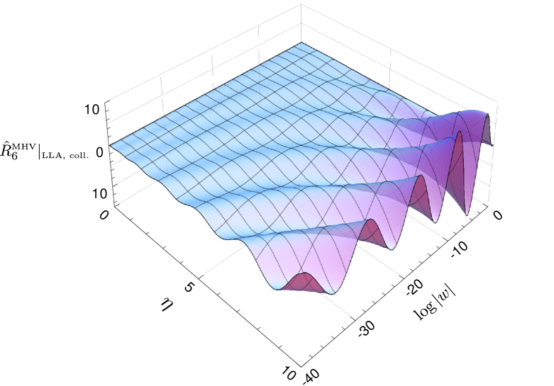
Figure 1: The MHV remainder function in the near-collinear limit of the LL approximation of MRK. It has been rescaled by an exponential damping factor. See eq. (5.12).

5.2 NMHV

A similar analysis can be performed for the NMHV helicity configuration. The situation is slightly more complicated in this case because the NMHV remainder function is not symmetric under conjugation $w\leftrightarrow{w^{\ast}}$. One consequence is that its expansion in the collinear limit requires two sequences of functions, which we choose to parameterize by $r_{k}^{\textrm{NMHV}}$ and $\tilde{r}_{k}^{\textrm{NMHV}}$,

$$\begin{split}R_{6}^{\textrm{NMHV}}|_{\textrm{LLA, coll.}}&\;=\;\frac{2\pi i}{\log(1-u_{1})}\Bigg{[}(w+{w^{\ast}})\sum_{k=0}^{\infty}\eta^{k+2}\,r_{k}^{\textrm{NMHV}}\!\big{(}\eta\log|w|\big{)}\\ &\hskip 106.69783pt+{w^{\ast}}\sum_{k=0}^{\infty}\eta^{k}\,\tilde{r}_{k}^{\textrm{NMHV}}\!\big{(}\eta\log|w|\big{)}\Bigg{]}\,.\end{split}$$ (5.13)

Contributions to the power series at order $w$ arise from the first term of eq. (4.3) (the second term has an overall factor of ${w^{\ast}}$), and, as in the MHV case, only from the subset of SVHPLs with a single $x_{1}$ in the weight vector. It is therefore possible to reuse eqs. (5.5)-(5.7) and obtain an explicit formula for the coefficient of $w$, $r_{k}^{\textrm{NMHV}}$. The result is,

$$r_{k}^{\textrm{NMHV}}(x)=\sum_{n=0}^{k}\sum_{m=0}^{n}\sum_{j=k-m}^{2k-n-m}\frac{(-2)^{2m+j-k}}{(m+j-k)!}\,\mathfrak{Z}(n,m)\,x^{m-k+(j-1)/2}\,P_{j+2}^{(k-j-n-1,k-j-m-1)}\big{(}0\big{)}\,I_{j+1}\big{(}2\sqrt{x}\,\big{)}\,.$$ (5.14)

The first few terms are

$$\begin{split}r_{0}^{\textrm{NMHV}}(x)&\;=\;-\frac{1}{4\sqrt{x}}I_{1}(2\sqrt{x})\,,\\ r_{1}^{\textrm{NMHV}}(x)&\;=\;-\frac{1}{8\sqrt{x}}I_{3}(2\sqrt{x})\,,\\ r_{2}^{\textrm{NMHV}}(x)&\;=\;\frac{3}{16x^{3/2}}I_{3}(2\sqrt{x})-\frac{1}{32\sqrt{x}}I_{5}(2\sqrt{x})\,.\end{split}$$ (5.15)

As previously mentioned, it is not so straightforward to extract the coefficient of ${w^{\ast}}$ in this way. We can instead make progress by exploiting the differential equation (2.21). In terms of the functions $r_{k}^{\textrm{MHV}}$, $r_{k}^{\textrm{NMHV}}$, and $\tilde{r}_{k}^{\textrm{NMHV}}$, the equations read,

$$\begin{split}\partial_{x}r_{k}^{\textrm{MHV}}(x)&\;=\;2\,r_{k}^{\textrm{NMHV}}(x)+\partial_{x}r_{k-1}^{\textrm{NMHV}}(x)\\ \partial_{x}\tilde{r}_{k}^{\textrm{NMHV}}(x)&\;=\;2\,r_{k}^{\textrm{MHV}}(x)+2\,r_{k-1}^{\textrm{NMHV}}(x)\,.\end{split}$$ (5.16)

The first of these equations is automatically satisfied and confirms the consistency of eq. (5.8) and eq. (5.14). The second equation determines $\tilde{r}_{k}^{\textrm{NMHV}}$ up to a constant of integration which can be determined by examining the $n=-1$ term of eq. (2.19). The solution is,

$$\tilde{r}_{k}^{\textrm{NMHV}}(x)=x\,\delta_{0,k}-\sum_{n=0}^{k}\sum_{m=0}^{n}\sum_{j=k-m}^{2k-n-m}\frac{(-2)^{2m+j-k}}{(m+j-k)!}\,\mathfrak{Z}(n,m)\,x^{m-k+(j+1)/2}\,P_{j}^{(k-j-n,k-j-m)}\big{(}0\big{)}\,I_{j-1}\big{(}2\sqrt{x}\,\big{)}\,.$$ (5.17)

The first few terms are

$$\begin{split}\tilde{r}_{0}^{\textrm{NMHV}}(x)&\;=\;x-\sqrt{x}\,I_{1}\left(2\sqrt{x}\right)\,,\\ \tilde{r}_{1}^{\textrm{NMHV}}(x)&\;=\;-\frac{1}{2}\sqrt{x}\,I_{1}\left(2\sqrt{x}\right)\,,\\ \tilde{r}_{2}^{\textrm{NMHV}}(x)&\;=\;\frac{1}{2\sqrt{x}}\,I_{1}\left(2\sqrt{x}\right)-\frac{1}{8}\sqrt{x}\,I_{3}\left(2\sqrt{x}\right)\,.\end{split}$$ (5.18)

Modified Bessel functions with even indices only appear in the $\zeta$-containing terms of $r_{k}^{\textrm{NMHV}}$ and $\tilde{r}_{k}^{\textrm{NMHV}}$. The explanation of this fact is the same as in the MHV case, except that the parity is flipped due to the shifts of the indices of the modified Bessel functions in eq. (5.14) and eq. (5.17).

5.3 The real part of the MHV remainder function in NLLA

As described in Section 2, the real part of the MHV remainder function in NLLA is related to its imaginary part in LLA. In the collinear limit, the relation (2.15) may be written as,

$$\begin{split}\textrm{Re}\left(R_{6}^{\textrm{MHV}}|_{\textrm{NLLA, coll.}}\right)&\;=\;\frac{2\pi i}{\log(1-u_{1})}\left(\frac{1}{2}\,\eta^{2}\,\frac{\partial}{\partial\eta}\,\frac{1}{\eta}-\frac{1}{2}\,\eta\log|w|\right)\,R_{6}^{\textrm{MHV}}|_{\textrm{LLA, coll.}}\\ &\quad-\frac{\pi^{2}}{\log^{2}(1-u_{1})}\eta^{2}\log|w|\,.\end{split}$$ (5.19)

Since $R_{6}^{\textrm{MHV}}|_{\textrm{LLA}}$ vanishes like $(w+{w^{\ast}})$ in the strict collinear limit, the quadratic term $(R_{6}^{\textrm{MHV}}|_{\textrm{LLA}})^{2}$ in eq. (2.15) only contributes to further power-suppressed terms in the near-collinear limit and is therefore omitted from eq. (5.19). We may write eq. (5.19) as,

$$\textrm{Re}\left(R_{6}^{\textrm{MHV}}|_{\textrm{NLLA, coll.}}\right)=-\frac{4\pi^{2}}{\log^{2}(1-u_{1})}(w+{w^{\ast}})\sum_{k=0}^{\infty}\eta^{k+1}q_{k}\big{(}\eta\log|w|\big{)}\,,$$ (5.20)

where,

$$q_{k}(x)=\frac{1}{4}\,x\,\delta_{0,k}+\frac{1}{2}\,(k-x)\,r_{k}^{\textrm{MHV}}\!\big{(}x\big{)}+\frac{1}{2}\,x\partial_{x}r_{k}^{\textrm{MHV}}\!\big{(}x\big{)}\,.$$ (5.21)

The leading term, $q_{0}$, corresponds to the real part of the next-to-double-leading-logarithmic approximation (NDLLA) of ref. [46]. Our results agree with that reference and read,

$$\textrm{Re}\left(R_{6}^{\textrm{MHV}}|_{\textrm{NDLLA}}\right)\;=\;\frac{\pi^{2}\,(w+{w^{\ast}})\,\eta}{\log^{2}(1-u_{1})}\,\left[-\eta\log|w|I_{0}\left(2\sqrt{\eta\log|w|}\right)+\sqrt{\eta\log|w|}\,I_{1}\left(2\sqrt{\eta\log|w|}\right)\right]\,.$$ (5.22)

6 Conclusions

In this article, we studied the six-point amplitude of planar ${\mathcal{N}}=4$ super-Yang-Mills theory in the leading-logarithmic approximation of multi-Regge kinematics. In this limit, the remainder function assumes a particularly simple form, which we exposed to all loop orders in terms of the single-valued harmonic polylogarithms introduced by Brown. The SVHPLs provide a natural basis of functions for the remainder function in MRK because the single-valuedness condition maps nicely onto a physical constraint imposed by unitarity. Previously, these functions had been used to calculate the remainder function in LLA through ten loops. In this work, we extended these results to all loop orders.

In MRK, the tree amplitudes in the MHV and NMHV helicity configurations are identical. This observation motivates the definition of an NMHV remainder function in analogy with the MHV case. We examined both remainder functions in this article, and proposed all-order formulas for each case. In fact, these formulas are related: as described in ref. [39], the two remainder functions are linked by a simple differential equation. We employed this differential equation to verify the consistency of our results.

We also investigated the behavior of our formulas in the near-collinear limit of MRK. The additional large logarithms that arise in this limit impose a hierarchical organization of the resulting expansions. We derived explicit all-orders expressions for the terms of this logarithmic expansion. The results are given in terms of modified Bessel functions.

We did not provide a proof of the all-orders result, but we verified that it agrees through 14 loops with an integral formula of Lipatov and Prygarin. The agreement of these formulas at 12 loops and beyond requires an intricate cancellation of multiple zeta values. It would be interesting to understand the mechanism of this cancellation. There are several other potential directions for future research. For example, in refs. [53, 54, 55], Alday, Gaiotto, Maldacena, Sever, and Vieira performed an OPE analysis of hexagonal Wilson loops which in principle should provide additional cross-checks of our results. It should also be possible to study the all-orders formula as a function of the coupling and, in particular, to examine its strong-coupling expansion. We have begun this study in the collinear limit and presented our initial results in Figure 1. A first attempt to compare the six-point remainder function in MRK at strong and weak coupling was made by Bartels, Kotanski, and Schomerus [32]. Further analysis of our all-orders formula should allow for an important comparison with this string-theoretic calculation.

References

• [1] Z. Bern, L. J. Dixon, D. C. Dunbar and D. A. Kosower, Nucl. Phys. B 425, 217 (1994) [hep-ph/9403226]; Nucl. Phys. B 435, 59 (1995) [hep-ph/9409265].
• [2] R. Britto, F. Cachazo and B. Feng, “New recursion relations for tree amplitudes of gluons,” Nucl. Phys. B 715, 499 (2005) [hep-th/0412308].
• [3] R. Britto, F. Cachazo, B. Feng and E. Witten, “Direct proof of tree-level recursion relation in Yang-Mills theory,” Phys. Rev. Lett.  94, 181602 (2005) [hep-th/0501052].
• [4] N. Arkani-Hamed, J. L. Bourjaily, F. Cachazo, S. Caron-Huot and J. Trnka, “The All-Loop Integrand For Scattering Amplitudes in Planar N=4 SYM,” JHEP 1101, 041 (2011) [arXiv:1008.2958 [hep-th]].
• [5] N. Arkani-Hamed, J. L. Bourjaily, F. Cachazo and J. Trnka, “Local Integrals for Planar Scattering Amplitudes,” JHEP 1206, 125 (2012) [arXiv:1012.6032 [hep-th]].
• [6] Z. Bern, J. J. M. Carrasco and H. Johansson, “New Relations for Gauge-Theory Amplitudes,” Phys. Rev. D 78, 085011 (2008) [arXiv:0805.3993 [hep-ph]].
• [7] Z. Bern, J. J. M. Carrasco and H. Johansson, “Perturbative Quantum Gravity as a Double Copy of Gauge Theory,” Phys. Rev. Lett.  105, 061602 (2010) [arXiv:1004.0476 [hep-th]].
• [8] K. T. Chen, “Iterated path integrals,” Bull. Amer. Math. Soc. 83 (1977) 831.
• [9] F. Brown, “Multiple zeta values and periods of moduli spaces $M_{0,n}$,” Annales scientifiques de l’ENS 42, fascicule 3, 371 (2009) [math/0606419].
• [10] A. B. Goncharov, “A simple construction of Grassmannian polylogarithms,” [arXiv:0908.2238].
• [11] A. B. Goncharov, M. Spradlin, C. Vergu and A. Volovich, “Classical polylogarithms for amplitudes and Wilson loops,” Phys. Rev. Lett.  105 (2010) 151605 [arXiv:1006.5703 [hep-th]].
• [12] C. Duhr, H. Gangl and J. R. Rhodes, “From polygons and symbols to polylogarithmic functions,” arXiv:1110.0458 [math-ph].
• [13] L. F. Alday and J. M. Maldacena, “Gluon scattering amplitudes at strong coupling,” JHEP 0706, 064 (2007) [arXiv:0705.0303 [hep-th]].
• [14] J. M. Drummond, J. Henn, V. A. Smirnov and E. Sokatchev, “Magic identities for conformal four-point integrals,” JHEP 0701, 064 (2007) [hep-th/0607160].
• [15] Z. Bern, M. Czakon, L. J. Dixon, D. A. Kosower and V. A. Smirnov, “The four-loop planar amplitude and cusp anomalous dimension in maximally supersymmetric Yang-Mills theory,” Phys. Rev. D 75, 085010 (2007) [hep-th/0610248].
• [16] J. M. Drummond, G. P. Korchemsky and E. Sokatchev, “Conformal properties of four-gluon planar amplitudes and Wilson loops,” Nucl. Phys. B 795, 385 (2008) [arXiv:0707.0243 [hep-th]].
• [17] A. Brandhuber, P. Heslop and G. Travaglini, “MHV amplitudes in ${\mathcal{N}}=4$ super Yang-Mills and Wilson loops,” Nucl. Phys. B 794, 231 (2008) [arXiv:0707.1153 [hep-th]].
• [18] L. F. Alday and J. Maldacena, “Comments on gluon scattering amplitudes via AdS/CFT,” JHEP 0711, 068 (2007) [arXiv:0710.1060 [hep-th]].
• [19] J. M. Drummond, J. Henn, G. P. Korchemsky and E. Sokatchev, “Conformal Ward identities for Wilson loops and a test of the duality with gluon amplitudes,” Nucl. Phys. B 826, 337 (2010) [arXiv:0712.1223 [hep-th]].
• [20] J. M. Drummond, J. Henn, G. P. Korchemsky and E. Sokatchev, “Dual superconformal symmetry of scattering amplitudes in ${\mathcal{N}}=4$ super-Yang-Mills theory,” Nucl. Phys. B 828, 317 (2010) [arXiv:0807.1095 [hep-th]].
• [21] J. M. Drummond, J. M. Henn and J. Plefka, “Yangian symmetry of scattering amplitudes in ${\mathcal{N}}=4$ super Yang-Mills theory,” JHEP 0905, 046 (2009) [arXiv:0902.2987 [hep-th]].
• [22] J. M. Drummond, J. Henn, G. P. Korchemsky and E. Sokatchev, “On planar gluon amplitudes/Wilson loops duality,” Nucl. Phys. B 795, 52 (2008) [arXiv:0709.2368 [hep-th]].
• [23] Z. Bern, L. J. Dixon and V. A. Smirnov, “Iteration of planar amplitudes in maximally supersymmetric Yang-Mills theory at three loops and beyond,” Phys. Rev. D 72, 085001 (2005) [hep-th/0505205].
• [24] Z. Bern, L. J. Dixon, D. A. Kosower, R. Roiban, M. Spradlin, C. Vergu and A. Volovich, “The two-loop six-gluon MHV amplitude in maximally supersymmetric Yang-Mills theory,” Phys. Rev. D 78, 045007 (2008) [arXiv:0803.1465 [hep-th]].
• [25] J. M. Drummond, J. Henn, G. P. Korchemsky and E. Sokatchev, “Hexagon Wilson loop = six-gluon MHV amplitude,” Nucl. Phys. B 815, 142 (2009) [arXiv:0803.1466 [hep-th]].
• [26] J. Bartels, L. N. Lipatov and A. Sabio Vera, “BFKL pomeron, Reggeized gluons and Bern-Dixon-Smirnov amplitudes,” Phys. Rev. D 80 (2009) 045002 [arXiv:0802.2065 [hep-th]].
• [27] V. Del Duca, C. Duhr and V. A. Smirnov, “An analytic result for the two-loop hexagon Wilson loop in ${\mathcal{N}}=4$ SYM,” JHEP 1003, 099 (2010) [arXiv:0911.5332 [hep-ph]].
• [28] V. Del Duca, C. Duhr and V. A. Smirnov, “The two-loop hexagon Wilson loop in ${\mathcal{N}}=4$ SYM,” JHEP 1005, 084 (2010) [arXiv:1003.1702 [hep-th]].
• [29] J. Bartels, L. N. Lipatov and A. Sabio Vera, “${\mathcal{N}}=4$ supersymmetric Yang Mills scattering amplitudes at high energies: the Regge cut contribution,” Eur. Phys. J. C 65 (2010) 587 [arXiv:0807.0894 [hep-th]].
• [30] R. M. Schabinger, “The imaginary part of the ${\mathcal{N}}=4$ super-Yang-Mills two-loop six-point MHV Amplitude in multi-Regge kinematics,” JHEP 0911, 108 (2009) [arXiv:0910.3933 [hep-th]].
• [31] L. N. Lipatov and A. Prygarin, “Mandelstam cuts and light-like Wilson loops in ${\mathcal{N}}=4$ SUSY,” Phys. Rev. D 83 (2011) 045020 [arXiv:1008.1016 [hep-th]].
• [32] J. Bartels, J. Kotanski and V. Schomerus, “Excited Hexagon Wilson Loops for Strongly Coupled N=4 SYM,” JHEP 1101, 096 (2011) [arXiv:1009.3938 [hep-th]].
• [33] L. N. Lipatov and A. Prygarin, “BFKL approach and six-particle MHV amplitude in ${\mathcal{N}}=4$ super Yang-Mills,” Phys. Rev. D 83 (2011) 125001 [arXiv:1011.2673 [hep-th]].
• [34] J. Bartels, L. N. Lipatov and A. Prygarin, “MHV amplitude for $3\to 3$ gluon scattering in Regge limit,” Phys. Lett. B 705 (2011) 507 [arXiv:1012.3178 [hep-th]].
• [35] L. J. Dixon, J. M. Drummond and J. M. Henn, “Bootstrapping the three-loop hexagon,” JHEP 1111 (2011) 023 [arXiv:1108.4461 [hep-th]].
• [36] V. S. Fadin and L. N. Lipatov, “BFKL equation for the adjoint representation of the gauge group in the next-to-leading approximation at ${\mathcal{N}}=4$ SUSY,” Phys. Lett. B 706 (2012) 470 [arXiv:1111.0782 [hep-th]].
• [37] A. Prygarin, M. Spradlin, C. Vergu and A. Volovich, “All two-loop MHV amplitudes in multi-Regge kinematics from applied symbology,” arXiv:1112.6365 [hep-th].
• [38] J. Bartels, A. Kormilitzin, L. N. Lipatov and A. Prygarin, “BFKL approach and $2\to 5$ MHV amplitude,” arXiv:1112.6366 [hep-th].
• [39] L. Lipatov, A. Prygarin and H. J. Schnitzer, “The multi-Regge limit of NMHV amplitudes in ${\mathcal{N}}=4$ SYM theory,” arXiv:1205.0186 [hep-th].
• [40] L. J. Dixon, C. Duhr and J. Pennington, “Single-valued harmonic polylogarithms and the multi-Regge limit,” arXiv:1207.0186 [hep-th].
• [41] J. Bartels, V. Schomerus and M. Sprenger, “Multi-Regge Limit of the n-Gluon Bubble Ansatz,” arXiv:1207.4204 [hep-th].
• [42] F. C. S. Brown, “Single-valued multiple polylogarithms in one variable,” C. R. Acad. Sci. Paris, Ser. I 338 (2004).
• [43] R. C. Brower, H. Nastase, H. J. Schnitzer and C.-I. Tan, “Implications of multi-Regge limits for the Bern-Dixon-Smirnov conjecture,” Nucl. Phys. B 814, 293 (2009) [arXiv:0801.3891 [hep-th]].
• [44] R. C. Brower, H. Nastase, H. J. Schnitzer and C.-I. Tan, “Analyticity for Multi-Regge Limits of the Bern-Dixon-Smirnov Amplitudes,” Nucl. Phys. B 822, 301 (2009) [arXiv:0809.1632 [hep-th]].
• [45] V. Del Duca, C. Duhr and E. W. N. Glover, “Iterated amplitudes in the high-energy limit,” JHEP 0812, 097 (2008) [arXiv:0809.1822 [hep-th]].
• [46] J. Bartels, L. N. Lipatov and A. Prygarin, “Collinear and Regge behavior of $2\to 4$ MHV amplitude in ${\mathcal{N}}=4$ super Yang-Mills theory,” arXiv:1104.4709 [hep-th].
• [47] N. Beisert, B. Eden and M. Staudacher, “Transcendentality and crossing,” J. Stat. Mech.  0701, P01021 (2007) [hep-th/0610251].
• [48] S. Moch, P. Uwer and S. Weinzierl, “Nested sums, expansion of transcendental functions and multiscale multiloop integrals,” J. Math. Phys.  43 (2002) 3363 [hep-ph/0110083].
• [49] V. Del Duca, “Equivalence of the Parke-Taylor and the Fadin-Kuraev-Lipatov amplitudes in the high-energy limit,” Phys. Rev. D 52, 1527 (1995) [hep-ph/9503340].
• [50] E. Remiddi and J. A. M. Vermaseren, “Harmonic polylogarithms,” Int. J. Mod. Phys. A 15 (2000) 725 [hep-ph/9905237].
• [51] L. Euler, Novi Comm. Acad. Sci. Petropol. 20, 140 (1775).
• [52] D. Zagier, “Values of zeta functions and their applications,” in First European Congress of Mathematics (Paris, 1992), Vol. II, A. Joseph et. al. (eds.), Birkhäuser, Basel, 1994, pp. 497-512.
• [53] L. F. Alday, D. Gaiotto, J. Maldacena, A. Sever and P. Vieira, “An Operator Product Expansion for Polygonal null Wilson Loops,” JHEP 1104, 088 (2011) [arXiv:1006.2788 [hep-th]].
• [54] D. Gaiotto, J. Maldacena, A. Sever and P. Vieira, “Bootstrapping Null Polygon Wilson Loops,” JHEP 1103, 092 (2011) [arXiv:1010.5009 [hep-th]].
• [55] D. Gaiotto, J. Maldacena, A. Sever and P. Vieira, “Pulling the straps of polygons,” JHEP 1112, 011 (2011) [arXiv:1102.0062 [hep-th]].