Distribution of entanglement in large-scale quantum networks
Abstract
The concentration and distribution of quantum entanglement is an essential ingredient in emerging quantum information technologies. Much theoretical and experimental effort has been expended in understanding how to distribute entanglement in one-dimensional networks. However, as experimental techniques in quantum communication develop, protocols for multi-dimensional systems become essential. Here, we focus on recent theoretical developments in protocols for distributing entanglement in regular and complex networks, with particular attention to percolation theory and network-based error correction.
type:
Review Articlepacs:
03.67.Bg, 03.67.Hk, 03.67.Pp, 03.67.Mn, 64.60.ah1 Introduction
The idea of quantum entanglement has a long history [1, 2, 3, 4], although an intensive search for a comprehensive theory of entanglement only arose with quantum information theory. This search grew out of the realisation that quantum entanglement is an essential resource for developing information technologies that are radically different than those possible in a purely classical world. In fact, when two physical systems are sufficiently entangled, they exhibit correlations that are stronger than possible with any classical theory. These strong correlations can then be exploited by cryptographic, communication, or computation protocols. As with classical information theory, there is a fundamental need to understand how to distribute information, that is, how to transmit a signal between two parties. But quantum mechanics imposes severe limitations, both fundamental and practical, on copying, encoding, and reading information. Thus, distributing quantum entanglement is an extremely challenging problem. This review presents work that attempts to meet that challenge.
Knowledge of the network in which this entanglement distribution will take place is still in a nascent stage. Naturally, most attention was initially focused on one-dimensional setups [5, 6, 7]. However, it is natural to consider distribution on multi-dimensional or otherwise more highly-connected networks, whose structure may be designed explicitly for distribution or be imposed by geographical constraints. Obvious examples of connections to existing bodies of work that will become increasingly important are the classical theory of complex networks, particularly those with an internet-like structure [8, 9, 10, 11]. From another point of view, the production and manipulation of entanglement on micro- or nano-scale networks is progressing rapidly [12]. In this case, we will likely be presented with regular arrays of elements that can be entangled. Both of these kinds of systems, and others not yet imagined, will require an understanding of entanglement distribution.
In any communication application, information is encoded in the state of a physical system. As this system travels from the sender to the receiver, it interacts with the environment, and a degradation or eventually a loss of information may occur. In classical systems, devices such as amplifiers have been specially developed to overcome this problem, by repeatedly copying the information content that is being transmitted. However, when single atoms or photons are used as information carriers, one faces a fundamental property of quantum mechanics which makes quantum communication challenging: quantum information cannot be copied perfectly [13]. On the other hand, quantum entanglement opens new possibilities in manipulation of information that are fundamentally impossible in the classical theory [14].
Before giving a detailed description of entanglement, we briefly review a few of the most important applications of this phenomenon; we refer the reader to [15] for a more complete review. These examples will repeatedly refer to the fundamental quantum system for quantum information science, the qubit, which is used as a quantum analogue of the classical binary digit or bit. The qubit is an abstraction that is realised by any two-level quantum system: the spin of an electron or neutron, the polarisation of a photon, or the first two energy levels of an atomic electron in a resonant field, just to name a few. These systems can be considered to have a single, two-dimensional degree of freedom, which means that, for a given orientation of the measurement device, a measurement always gives one of two results.
Quantum teleportation
It has been proven that the unitary evolution of quantum mechanics implies that an unknown quantum state cannot be duplicated or cloned [13]. However, an unknown quantum state can be transported over an arbitrarily long distance as long as an auxiliary perfectly entangled pair of particles (also called a Bell pair) and a classical communication channel are established over the same distance [16]. The entangled pair is created via a local temporary interaction between two qubits, which are then separated by the desired distance. The procedure is as follows. Two distant parties, traditionally called Alice and Bob, share an entangled pair of qubits, while Alice has an additional “data” qubit that she wishes to send to Bob. Alice performs a certain measurement on the two qubits she possesses and communicates the result classically to Bob. Bob then applies a transformation on his qubit in a manner prescribed by the message from Alice. The result is that Bob’s qubit is now in the original state of the data qubit of Alice, which meanwhile has lost its information content.
Quantum distributed computing
Distributed computing consists of several nodes that do computations independently while periodically sharing results. Entanglement appears in several places in quantum distributed computing protocols, including in the input states or in the communication channels used in sharing results between nodes. Attempts have been made to design quantum distributed computers so that limited entanglement resources are spread in an optimal way among components [17].
Quantum key distribution
Classical public key cryptography schemes are widely used, for instance, in internet security algorithms. Entangled pairs can be used to securely generate and distribute the classical private key necessary for these schemes [18, 19] (although performing quantum key distribution without distributing entanglement is also possible [20]). Using a quantum protocol, Alice and Bob generate a series of random bits, sharing knowledge of the results, but preventing others from eavesdropping. To this end, they initially share a number of Bell pairs, which they measure sequentially, each time choosing an orientation randomly from a pre-determined set. They can use a portion of their results to compute a bound on the amount of eavesdropping (or noise) that has taken place, and another portion to generate the key.
Superdense coding
If two parties share a Bell pair, then two classical bits of information can be sent from one party to the other one, even though each party physically possesses only one qubit [21]. To accomplish this, Alice applies one of four previously agreed-upon unitary operations to her qubit. A unitary operation, in contrast to measurement, transforms the qubit in a non-destructive and coherent way. This transforms the Bell state to one of four orthogonal states that together form the Bell basis. Alice sends her qubit to Bob, who then performs a joint measurement on both qubits, thus distinguishing reliably among the four messages Alice can send.
Each of the applications mentioned above requires entangled pairs of particles to be generated and distributed between two distant parties. Currently, the main technological difficulty is to create remote entanglement which, in most experiments, is achieved by sending polarised photons through optical fibres. In fact, due to noise, scattering, and absorption, the probability that the quantum information contained in such photons reaches its destination decreases exponentially with the distance. Another experimental challenge is to transfer the quantum state of the photon onto that of a quantum memory, such that the entanglement can be manipulated and stored; see [22] for a recent review on quantum memories.
Outline
We first review some well-known results on entanglement and describe the operations that allow one to propagate quantum information in a network, such as entanglement purification and entanglement swapping; see section 2.1.2 and section 2.2 [15]. Based on these operations, the quantum repeaters enable entanglement to be generated over a large distance in one-dimensional networks [5]; see section 2.3. However, in order to obtain reasonable communication rates, they require an amount of entanglement per link of the network that increases with the distance over which one would like to distribute entanglement, which is out of reach with present technologies. A natural question is whether the higher connectivity of the stations or nodes of more complex networks can provide some advantage over a one-dimensional setup when distributing entanglement; see section 3. The first protocol exploiting this fact uses ideas of percolation in two-dimensional lattices: for pure states, if enough entanglement is generated between neighbouring stations, then it can be propagated over infinite distance [23]; see section 3.2. For general mixed states, i.e. quantum states that contain random noise, this result no longer holds. For some specific types of noise, however, entanglement percolation still allows entanglement to be generated between infinitely distant stations [24, 25]; see section 3.3.
It turns out that all percolation strategies need, in the end, perfect operations to be applied on the system. The study of strategies with perfect operations is certainly useful, for instance in establishing fundamental limits. Still, we must ask if the higher connectivity of quantum networks will be of practical use, given that, in realistic scenarios, operations are not perfect, but rather introduce noise. We will see that the answer to this question is positive. But, in order to accommodate noisy operations, radically different protocols, based on error correction, must be designed [26, 27, 28, 29, 30]; see section 4. In fact, while entanglement percolation relies on the existence of one path of perfectly entangled states between any two stations, network-based error correction extracts its information from all paths connecting the two stations. Contrary to the quantum repeaters, no quantum memory is needed in that case.
Initially applied to regular lattices, the study of entanglement distribution has since been extended to complex networks [31]; see section 5. This is a natural generalisation because present communication networks exhibit a complex structure. Furthermore, while mostly focused on pure states, recent work concerns the manipulation of entanglement in noisy quantum complex networks; see section 5.4. These results emphasise the fact that the quality of the quantum communication between two stations will depend greatly on our understanding of the interplay of the network topology and the quantum operations available on the system.
2 Concepts and methods
In this section we describe some well-known results on entanglement and the basic operations that are used to propagate quantum information in a network; see [32] for a thorough treatment of this material in a pedagogical setting. A reader familiar with quantum information theory may skip this part and jump to the discussion of quantum repeaters in section 2.3 or percolation in section 3.
2.1 Quantum states
The state of a single qubit can be written as
| (2.1) |
where and represent a choice of basis, called the computational basis, in a Hilbert space. Since the phase is irrelevant to the remainder of this review, we shall choose . We say that the system is in a coherent superposition of the two basis states. We can measure the state of the qubit in this basis, which corresponds, for instance, to the orientation of magnets acting on the spin of electrons in the laboratory. The probability that we measure is and the probability that we measure is . We must have , as these are the only possible outcomes. Upon measurement in the computational basis, the state of the system collapses into one of the two basis states, say . If we now repeat the same measurement, we have and , so that we obtain with probability . However, if we rotate our magnets to an orientation corresponding to a different basis and then measure, we must expand in that new basis in order to calculate the probabilities of obtaining each of the two possible results.
2.1.1 Measurements and quantum evolution
While the study of quantum measurement is a broad and deep subject, here we only need to introduce a few ideas to discuss entanglement distribution. Measurements occur in the laboratory, but the computational tool to predict their result associates with each type of measurement a set of linear operators on the state space. The measurements described above are called projective measurements, which are defined by a collection of projectors onto subspaces of the state space, each of which is associated with a possible measurement value. After measuring a value, we know that the system has collapsed into a state in the subspace corresponding to the associated projector. The projectors are orthogonal, and the requirement that we must get some result implies that their sum is the identity. The maximum number of orthogonal projectors is equal to the dimension of the state space and corresponds to a complete measurement. On the contrary, we use an incomplete measurement, with fewer projectors, when we want to extract only partial information from a state while preserving some property common to all subspaces. Finally, we will sometimes make use of generalised measurements, in which the condition that the operators are orthogonal is relaxed. Measurements are then defined by a collection of semi-definite positive operators that sum to the identity [14].
The other component of quantum theory that transforms states is evolution. Evolution is also represented theoretically by operators, but in contrast with measurement, an initial state is transformed into a final state in a deterministic way. Operators representing evolution must have the algebraic property of unitarity in order to conserve total probability. These operators are commonly referred to as unitaries. The entanglement distribution procedures in this review are built from a combination of measurements and unitaries on quantum states, together with classical communication.
2.1.2 Entanglement
To illustrate the basic idea of entanglement while making a connection with the remainder of this review, let us consider two qubits, i.e. two systems each of which consist of a two-level quantum state. Two qubits live in a four-dimensional state space whose computational basis is , where the first binary digit corresponds to qubit and the second to qubit . Mathematically, these basis vectors are tensor products of vectors in the local spaces: If the two systems have never interacted directly or indirectly, then each one has an independent description of its state, as in (2.1). In this case, it is possible to find local bases for each qubit such that the joint state is one of the four computational basis states of the joint space. These states are called product states. Measurements and operations applied on one system have no effect on subsequent measurement outcomes on the other system. However, suppose an interaction between the systems is turned on, then off. In general, there is no local basis such that the state of the system after the interaction can be written as a factor of states of the subsystems. A pure bipartite quantum state is then said to be entangled if it cannot be written as a tensor product. That is, it cannot be written as
| (2.2) |
A famous example of entangled states are the four Bell states
| (2.3a) | |||||
| (2.3b) | |||||
which form a basis of two-qubit systems. These states are of central importance as they are maximally entangled states. The projective measurement corresponding to the four states of the Bell basis is called a Bell measurement.
Just as two two-dimensional systems form a four-dimensional system, in general, the space describing a collection of quantum systems of dimensions has dimension . However, generalising the case of two qubits, we may partition any of these composite spaces into two subspaces, and viewed this way, the system is called a bi-partite system. The study of bi-partite entanglement, that is entanglement between the two subspaces, is far better understood than the more general case of multi-partite entanglement, and we shall mostly be concerned in this review with bi-partite systems.
Until now, we have discussed only what are known as pure quantum states, in which the probability of measuring a value is of local quantum mechanical origin. However, the generic case is that the system is entangled with other systems which we cannot measure. It turns out that to predict local measurements in this case, we can assume that the local state is effectively a classical distribution of several pure states, and can be written as
where is a probability distribution. This classical ensemble of pure states is known as a mixed state. It is important to realise, however, that this decomposition is not unique. These states are described not by vectors in the Hilbert space of pure states, but rather by linear operators known as density operators, which act on the same Hilbert space. For instance the density operator corresponding to a pure state is given by the outer product of the pure state vector with itself, which is denoted by . Rules of quantum mechanics together with classical statistics imply that density operators must be non-negative and have trace one. The set of operators on finite-dimensional Hilbert spaces may be represented by a set of matrices that depends on a chosen basis. Since all systems considered in this review are composed of locally finite-dimensional Hilbert spaces, we follow the common practice of using the term density matrix even if the choice of basis is not fixed.
The notion of entanglement can be easily generalised to mixed states [33]. In this case, a bi-partite system is entangled if and only if its joint density operator cannot be written
| (2.3d) |
that is, it is not a mixture of product states.
Measures of entanglement
If one qubit of a Bell pair is measured in the computational basis, that is, if it is projected onto the eigenstates and of the Pauli matrix, then the measurement outcome is either 0 or 1 with equal probabilities. If the second qubit is then measured in the same basis, the outcome is completely determined by the first result. But, if we instead were to measure each qubit in the same arbitrary rotated basis, the same correlation between outcomes would be seen. In fact, it can be shown that the Bell states are the maximally-correlated two-qubit states; they are maximally entangled. In operational terms this means that they can be used to teleport perfectly the state of exactly one qubit. In practice, however, the entanglement between two qubits is never perfect, so that partially entangled states have to be considered. In what follows we present some common measures of entanglement.
In the pure-state formalism, local bases may be found so that any two-qubit state is written
| (2.3e) |
where the two Schmidt coefficients and satisfy and (by convention). If one of the coefficients or vanishes, the system is separable. If , it is maximally entangled. Otherwise, the system is said to be partially or weakly entangled. An important measure of entanglement is
| (2.3f) |
which corresponds to the optimum probability of successfully converting into a perfect Bell pair by local operations [34]; see section 2.2.3.
Another common measure of entanglement, the concurrence [36], reads in the case of pure states:
| (2.3g) |
For mixed state one can generalise the concurrence in a similar way as done for the entropy of entanglement. The mixed state of two qubits is represented by a four-by-four density matrix, which requires, in general, fifteen parameters. Any density matrix of two qubits can be transformed by local random operations to the standard form
| (2.3h) |
where is the corresponding identity matrix. This process is known as depolarisation, and is called a Werner state. It is important to notice that the depolarisation process typically increases the entropy of the system and reduces its entanglement. One sometimes explicitly expands this expression in the Bell basis :
| (2.3i) |
where the components correspond to the weight of each Bell state in the mixed state decomposition of . Although depolarisation may decrease entanglement, it is done in a way that preserves the fidelity with respect to a preferred state [37]:
| (2.3j) |
This fact is important because the concurrence of the Werner state is related to the fidelity via
| (2.3k) |
The state is entangled if and only if its concurrence is strictly positive, that is if ; or equivalently, if
| (2.3l) |
Note that (2.3h) emphasises the fact that a Werner state is a mixture of a perfect quantum connection and a completely unknown state. This observation is important, for instance, when discussing the limitations of entanglement propagation in noisy networks; see section 3.4. The Werner state is an example of a full-rank state, that is, one with no vanishing eigenvalues. Full-rank states result from a general noise model and are thus important because they model any state found in a laboratory. However, the entanglement contained in these states cannot be extracted easily, and special techniques have to be developed to this aim; see section 2.2.3.
The discussion to this point may leave the reader with the impression that characterisation of entanglement is a relatively uncomplicated task. In fact it is a difficult and deep question, especially for mixed and multipartite states [38]. On one hand a separable state can be written as a classical mixture of projectors onto product states. On the other hand, there is no general algorithm to determine whether a given density operator can be written in this form, although significant progress has been made [39, 15].
2.2 Entanglement manipulation in quantum networks
In the introduction, we have seen that entanglement is a valuable resource for a variety of quantum information applications. It is thus essential to understand the non-trivial task of creating and distributing entanglement between distant parties. The subject is greatly complicated, in fact largely determined, by the fact that entanglement is a very fragile resource, in the sense that it inevitably deteriorates while being manipulated or stored. We shall see that the attempt to overcome this difficultly has led naturally to the consideration of network theory.
The most direct way to produce entanglement between spatially separated parties is to entangle two particles locally and then to send one of them physically to another location. Most research in this direction involves sending photons through optical fibres, which suffer from inherent limitations due to photon loss via absorption as well as coherence of the state. The limit at this time is about 100 km [40], because the probability of transmission decays exponentially with the distance, becoming as low as for km [41]. Following the techniques developed in classical systems in order to overcome similar but much less severe limitations, creating entanglement between distant stations via a series of intermediate nodes has been proposed. The main and crucial difference with classical information is that qubits cannot be copied, so that the intermediate links have to be joined together in a very subtle way, known as entanglement swapping, which will be discussed below. This one-dimensional system of links and nodes has then a natural generalisation to a network of arbitrary geometry.
2.2.1 Structure of quantum networks
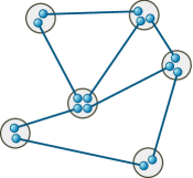
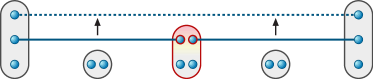
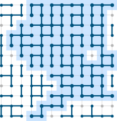
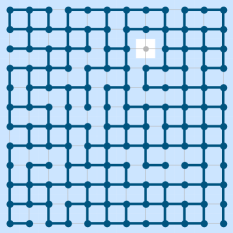
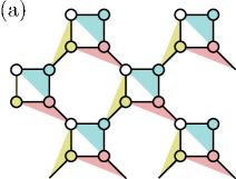
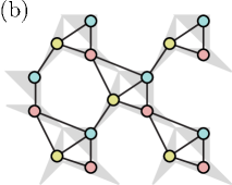
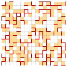
The quantum networks that we consider consist of two basic elements: nodes (or stations), each of which possesses one or more qubits; and links, each of which represents entanglement between qubits on different nodes. This generalises the one-dimensional scenario in that links may exist between all pairs of nodes, rather than only neighbouring nodes on a chain. An example of such a quantum network is shown in figure 1. It is often useful to interpret this structure in terms of graph theory, where the nodes become vertices and the links become edges. Furthermore, we sometimes use the language of statistical physics by referring to a regular graph with local connections as a lattice.
2.2.2 Local operations and classical communication
In manipulating entanglement in a quantum system, we typically begin with a given distribution of entangled pairs of qubits and then apply a series of operations designed to distribute the entanglement in a useful way. The problems we consider naturally impose a distinction between local and distributed resources. It is important to have a clear notion of what kind of operations are allowed on these resources. In this review, we shall only consider local operations and classical communication (LOCC) on the network. It turns out that it is possible to provide an operational definition of entanglement as the quantum resource that does not increase under LOCC. It is easy to see that this definition is equivalent to the pure mathematical one given by (2.3d).
It is now clear how the concept of LOCC leads to the quantum network shown in figure 1. Recall that the network initially is composed of some entangled pairs of qubits, with one party of each pair occupying a node of the network. However, several qubits from different pairs occupy a single node along with other possible resources, both quantum and classical. When we speak of local operations and resources, we mean quantum operations and resources within each node. On the other hand, we allow only classical messages to be sent between the nodes. Qubits belonging to different nodes cannot interact quantum mechanically, so that no further entanglement can be created between remote stations. However, qubits within a node may interact in any way, including with ancillary (local) resources, and any measurement may be performed on the components of the node.
2.2.3 Purification of weakly entangled states
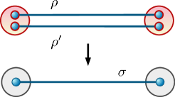
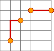
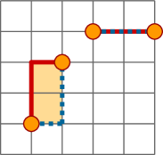
We now address the task of concentrating or purifying the entanglement of two (or more) weakly entangled states into a pair with higher entanglement, using LOCC only. Suppose that these states are arranged in a parallel fashion so that local operations may be performed jointly on all left-hand members and on all right-hand members as shown in figure 2. An important task is to find criteria determining when and how a given set of states can be transformed into a more highly-entangled target state.
Pure states
Majorisation theory was developed to answer the question: What does it mean to say one probability distribution is more disordered than another? One application to quantum mechanics is via the connection between disorder (of the Schmidt coefficients) and entanglement. Consider an initial pure state and a target state in a bipartite system. These states may have any dimension , that is, they are pairs of qudits. Denoting by the unit vector of the Schmidt coefficients of sorted in decreasing order (and similarly for ), Nielsen showed in [42] that a deterministic LOCC transformation from to is possible if and only if the inequalities
| (2.3m) |
hold for all . In this case, is said to be majorised by , which is denoted by ; see [43] for more details on this topic. Note, for instance, that the maximally entangled state can be deterministically transformed into any other pure state. As another example, consider setting for the two pure states and depicted in figure 2, so that one finds . In this case, the two pairs of qubits can be transformed into a single connection if and only if .
Moving now to non-deterministic transformations, the optimal probability for a successful LOCC conversion is [34]:
| (2.3n) |
Using this formula, it is trivial to check that a two-qubit pure state can be transformed into a Bell pair with optimal probability , as stated in section 2.1.2. Explicitly, this result is obtained by performing on one of the qubits a generalised measurement defined by the operators
| (2.3o) |
which is known as the “Procrustean method” of entanglement concentration [44].
Mixed states
The purification of mixed states is a somewhat more difficult problem than that of pure states. Many techniques have been developed for doing mixed-state entanglement purification in connection to quantum error-correction [35]. For our purpose, it is sufficient to notice that:
-
1.
In contrast with the case of pure states, at least two copies of a Werner state are needed to get, by LOCC and with finite probability, a state of higher fidelity [46].
-
2.
Perfect Bell pairs can be obtained from Werner states only in the limit [47].
The first purification scheme, which was proposed by Bennett et alin [37], is depicted in figure 2: the two states and are purified into the state , with
| (2.3p) |
The resulting state is closer to the target state if both and are entangled (that is, if ) and if . It is important to note that this operation is not deterministic since it succeeds only with probability
| (2.3q) |
This procedure can be iterated, with increasing after each step, until it is arbitrarily close to (considering perfect operations); this asymptotic technique is sometime referred as distillation. However, one is often interested in the yield, which is defined as the asymptotic ratio of the number of input states to the number of output states. The above protocol requires a diverging number of states to produce one arbitrarily pure state, and thus has a vanishing yield. In order to get a positive yield, the previous method is applied until states of sufficiently large are generated, and then one switches to purification techniques using one-way communication. Many improvements and variants over this construction exist; see [15, 45] and references therein.
2.2.4 Entanglement swapping
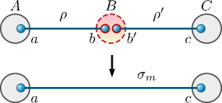
The basic operation to propagate the entanglement in a quantum network is the so-called entanglement swapping [16, 50, 51, 52] depicted in figure 3: By performing a Bell measurement on the qubits and at the station , one creates a quantum link between the previously unconnected stations and . Then, a local unitary that depends on the outcome of the measurement is applied on the qubit , so that the resulting entangled pair has the standard form given in (2.3e) or in (2.3h). This operation is equivalent to teleporting to .
For two mixed states and , it is easy to see that the entanglement swapping produces the quantum state for all measurement outcomes, that is,
| (2.3r) |
In the case of pure states and , however, the result depends on the outcome, and one gets either a Bell pair or a state that is weakly entangled. Remarkably, the average entanglement of the resulting states is not less than that of the initial states:
| (2.3s) |
which is, for , the “conserved entanglement” described in [53]. This property of pure states will be used in the various protocols of entanglement propagation described in section 3.
Maximising the average entanglement of the outcomes is of prime importance for random or statistical processes. However, one may also desire that every possible outcome results in a state with a reasonable amount of entanglement. In this scenario one can use the rotated Bell basis to perform the entanglement swapping; see section 1.1 in [54]. In this case, one gets four outcomes satisfying
| (2.3ta) | |||
| or, equivalently, | |||
| (2.3tb) | |||
The entanglement swapping procedure can be iterated, creating a quantum connection between qubits that are more and more distant. However, the resulting long-distance entanglement that is generated in this way decreases exponentially with the number of swappings. This is clear in the case of mixed states and for pure-state Bell measurements in the basis; the general proof can be found in section 1.3 in [54]. Because of this important loss of entanglement, new schemes have to be designed to efficiently entangle any two stations of a quantum network. The various protocols proposed so far that achieve this task are described in the following chapters.
Noisy operations
Thus far, we have assumed that all quantum operations are ideal or perfect. However, in practice, every operation or measurement introduces some noise. Here we consider two sources of error: those arising from applying an imperfect gate (unitary operation), and those arising from an imperfect measurement. In the first case we model the error by including a small depolarising term to a channel, which replaces a fraction of the density operator with a completely decoherent (i.e. unknown) state [5, 54]. For a multi-qubit state, a gate acting on a subset of qubits with an error probability is replaced by the map
| (2.3tu) |
where denotes the partial trace over the subsystem , and is such that the resulting state has trace one. It can be shown that this model correctly models isotropic errors for single qubit rotations [6]. On the other hand, suppose we model a measurement error on a single qubit by assuming that we have a small fixed probability of reading when the qubit was actually measured into the state. In this case, the measurement operators read:
| (2.3tv) |
Propagating the errors according to this simple model allows us to estimate the error resulting from a particular protocol.
2.3 The quantum repeaters
A great deal of theoretical and experimental effort has been put forth to distribute entangled states over long distances using essentially one-dimensional lattices. As we mentioned above, networks were introduced to solve problems caused by unavoidable loss and decoherence through free-space and fibre links. In particular, quantum repeaters, which have entanglement swapping at their heart, have received the most attention.
The initial proposals for quantum repeaters use a hierarchical scheme of swapping and purification steps [55, 5, 6]. Including purification in the protocol is necessary once one introduces real-world noise and errors. Noise enters the system in two ways. First, each operation or measurement reduces the fidelity of the desired state. This noise is modelled as described in the previous section. Second, even in the case of perfect operations, if one begins with a slightly impure state, then the state resulting from a protocol decays rapidly in the number of operations, such as the swapping in (2.3r), to a useless separable state. As explained above, the losses suffered by a state transmitted through the links of the network increases exponentially with distance. This introduces a maximum length of elementary links because there is a minimum fidelity (2.3l) below which purification is impossible. The repeater protocol first prepares several states of along a relatively short link and stores them in quantum memories. Then they are used to produce a pair with higher fidelity through entanglement purification. Entanglement swapping is then performed on two of these purified states on neighbouring links thus creating entanglement across a distance that is twice the length of the elementary link. The noisy swapping again reduces the fidelity, so that more quantum memories and more purifications is needed. This procedure is iterated so that, in principle, highly entangled states can be created across long distances.
Based on the initial protocol for quantum repeaters, many improvements have been suggested; see [41] for a review on this topic. For instance, it has been shown that the number of qubits per station does not have to grow with the distance [7]. Yet, the realisation of quantum repeaters is still a very challenging task, which is mainly due to the need of reliable quantum memories [56].
2.3.1 Implementations
All building blocks needed to construct a quantum network have been demonstrated, and, in fact, small-scale quantum networks are now a reality. For instance, while the first demonstrations of teleportation were made in laboratory scales [50, 57, 58], presently, entangled photons distributed in free space can be used for teleportation over km [59, 60] (see also the recent improvements in the direction of telecommunication [61]). Moreover atom-photon interfaces have also been used in the demonstration of teleportation [62, 63] and entanglement swapping was also shown in different scenarios [64, 65].
One of the first implementations of a quantum network, the DARPA Quantum Network, consists of several nodes and supports both fibre-optic and free-space links [66]. It is capable of distributing quantum keys between sites separated by a few tens of kilometres. Another example is the SECOCQ network in Vienna, which consists of six nodes connected by links ranging from 6 to 85 km [67].
3 Entanglement percolation
An approach to entangling distant parties that is conceptually
different from the quantum repeater was proposed in [23]. In
this paper, the main question is: given a quantum network,
or graph, which operations should be performed on the nodes so that
entanglement is best propagated?
A first answer is presented in section 3.1:
for some graphs, the gain obtained from purification of weakly
entangled states can balance, or even surpass, the loss of
entanglement resulting from the swappings. This result is
promising, but it is merely an adaptation of the quantum repeater
protocol to specific graphs and quantum states. In fact, it
somewhat replaces the repeated generation of elementary links by a
deterministic accumulation of the entanglement of existing links,
provided that they are in a pure state,
or that the graph has a specific structure.
The solution proposed in [23] is of a different nature.
Its underlying idea is that in one-dimensional networks, any
defective link destroys the whole procedure, while in higher-dimensional
networks the information can still reach its destination through other paths.
This phenomenon is related to percolation theory, which states that if there
are not too many defective links in, say, a square lattice, then any two nodes
of the network are connected by a path with non-vanishing probability.
Strategies based on this idea are described in section 3.2. Initially
limited to pure states, they have since been generalised to some special cases
of mixed states; see section 3.3.
3.1 Deterministic protocols based on purification
In this section, we show that qubits can become entangled over large scales in some two-dimensional (planar) graphs, using predetermined sequences of entanglement swappings and purifications. Very close to the quantum repeaters in spirit, this method can be applied either with mixed states in a restricted class of graphs (section 3.1.1) or with pure states in lattices of high connectivity (section 3.1.2).
3.1.1 Hierarchical graphs

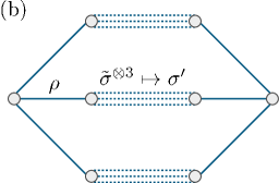
Hierarchical graphs iterate certain geometric structures, so that at each level of iteration either the number of neighbours or the length of the connections increases. Various such graphs were considered in [68]; let us give here yet another example in which both pure and mixed state entanglement can be generated between nodes that lie at any level of the hierarchy. In this example, two infinite ternary trees, in which each link is an entangled state , are connected at their leaves by a state ; see figure 5a. The protocol runs as follows: First, two entanglement swappings are performed on the central links , , and , yielding a state . Second, the three states that connect the new leaves of the ternary trees are purified, leading to a single connection . The procedure can be iterated as long as . In this way, nodes lying at higher and higher level of the hierarchical graphs become entangled, that is, larger and larger quantum connections are created. In the following, we determine the minimum amount of pure or mixed-state entanglement of and for this strategy to be successful.
Pure states
In section 2.2.4, we saw that the result of the entanglement swappings depends on the basis that is chosen for performing the two-qubit measurement. In order to facilitate the comprehension of the mechanism, we choose the basis, so that all outcomes are equally entangled: ; see (2.3tb). The optimal purification of into , as described in section 2.2.3, requires working with the Schmidt coefficient . One then finds , and the recursion relation for the entanglement of the central connections reads:
| (2.3ta) |
with and . In this equation, the parameter lies in the interval . It is an easy calculation to show that for any value of if , that is, if . This means that the entanglement cannot be propagated in the hierarchical graph if the links are too weakly entangled. In contrast, if , one stable and non-trivial fixed point appears in (2.3ta); see figure 6. In this case, nodes lying at any level of the hierarchy can be connected by an entangled state of two qubits; one further shows that this state is a perfect Bell pair if .

Mixed states
The scenario of a mixed-state hierarchical graph, where the connections are Werner states and , is quite similar to that of pure states. First, two consecutive entanglement swappings are performed on the central states , , and , leading to a state with . Then, we try to concentrate the entanglement of the three states into one connection . As for the pure states, we would like this operation to be deterministic, but the purification of mixed states is intrinsically probabilistic. In order to get a result in a predictable fashion, we purify two connections only and take the third one if the purification failed. From (2.3p) and (2.3q), this succeeds with probability and the average entanglement of is
| (2.3tb) |
If the links of the graph satisfy and , then a stable fixed point appears. In this case, iterating the entanglement swappings and the purifications generates some long-distance pairs of qubits whose entanglement approaches .
3.1.2 Regular graphs
We have just shown that entangled pairs of qubits can be generated over a large
distance in graphs with a hierarchical structure, under the condition that the
entanglement of the bonds if larger than a critical value . The self-similarity
of these graphs allows one to design natural sequences of entanglement swappings
and purifications but suffers a physical limitation: either the length of the
bonds or the number of qubits per node grows exponentially with the iteration depth.
We now consider regular two-dimensional lattices, that is, periodic
configurations of links throughout the plane in which the nodes have a fixed
number of neighbours.
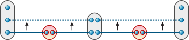
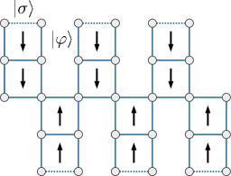
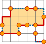
A deterministic strategy to entangle two infinitely distant nodes in lattices in which each node has a number of nearest neighbours was proposed in [68]. It is very similar to the recursive method developed in the previous example, but it works only with pure states. In the case of a square lattice of links , the idea is to sequentially shorten the legs of a “centipede”, so that the entanglement of the links is gradually concentrated; see figure 7. This eventually yields a perfect Bell pair at the spine of the centipede, on which infinitely many entanglement swappings can be applied, and therefore long-distance entangled pairs of qubits are generated. More precisely, one starts by applying two entanglement swappings in the basis on the states (dotted line in figure 7) and its neighbour states at the extremity of each leg. This results in a state , and as in the previous example, we have . The difference is that the purification is now performed on rather than on . Very similarly to (2.3ta), one finds the following recursion relation:
| (2.3tc) |
where is a function of . One can show that there always exists a non-trivial stable fixed point for this equation. However, the fixed point of (2.3tc) is strictly smaller than unity when . In this case, although we do concentrate some entanglement along the spine of the centipede, we still face the problem that the spine is a one-dimensional system, which therefore exhibits an exponential decrease of the entanglement with its length. On the other hand, if , then the fixed point is reached in a finite number of steps, and a maximally entangled state is generated. Since the spine now consists of perfect connections, any two nodes lying on it can share a Bell pair, regardless of their distance.
3.2 Percolation of partially entangled pure states
We have demonstrated that a way to generate long-distance entanglement in a lattice is to purify a “backbone” of Bell pairs and then to perform some entanglement swappings along this path. Three conditions have to be satisfied for this method to work. First, the nodes that belong to the backbone must have at least four neighbours each: two connections are part of the backbone, while the other two are used to purify the former. Second, the entanglement of the bonds has to be larger than a critical value that depends on the lattice geometry. Third, the links have to be pure states and not mixed states, because the purification of a finite number of Werner states never leads to a Bell pair (section 2.2.3). Since this deterministic strategy creates a chain of Bell pairs by using only a strip of finite width from the lattice, it seems that it does not exploit the full potential of two-dimensional networks. In this section, we review the method of entanglement percolation111Note that the probabilistic nature of quantum physics makes percolation theory a particularly well-adapted toolbox for the study of quantum systems which undergo, for instance, measurements. Ideas of percolation theory are for example useful in the context of quantum computing with non-deterministic quantum gates [69]. We refer the interested reader to pp. 287–319 in [70] for an overview of the application of percolation methods to the field of quantum information. that was published in [23] and that partially relaxes the above conditions:
-
1.
percolation is a genuine two- (or multi-) dimensional phenomenon, and thus it applies to any lattice;
- 2.
- 3.
The simplest application of entanglement percolation in infinite lattices is presented in section 3.2.1. In this case, the connection to classical percolation theory is straightforward and entanglement thresholds are readily determined. Then, we show that modified versions of this classical entanglement percolation (CEP) yield lower thresholds. For instance, we reconsider the hexagonal lattice with double bonds proposed in [23], in which quantum measurements lead to a local reduction of the entanglement but change the geometry of the lattice. This operation increases the connectivity of the graph and lowers the entanglement threshold, an effect which is called quantum entanglement percolation (QEP); see section 3.2.2. Finally, an alternative construction that uses multipartite entanglement is given in section 3.2.3. Using incomplete measurements, this protocol creates entangled states of more than two qubits and improves not only the entanglement threshold, but also the success probability of the protocol for any amount of entanglement in the connections for all the cases considered in section 3.2.3.
3.2.1 Classical entanglement percolation
Classical percolation is perhaps the fundamental example of
critical phenomena, since it is a purely statistical
one [72]. At the same time, it is quite universal
because it describes a variety of processes, with
applications in physics, biology, ecology, engineering,
etc. [73]. Two types of models are typical
considered, site- and bond percolation. In bond
percolation, the neighbouring nodes of a lattice are
connected by an open bond with probability ,
whereas they are left unconnected with probability ;
see figure 8. In site percolation, the
sites (i.e. nodes) rather than bonds are occupied with
probability . In either case, for an infinite lattice,
one would like to know whether an infinite open cluster
exists, that is, whether there is a infinitely long path of
connected nodes. It turns out that an unique infinite
cluster appears if, and only if, the connection
probability is larger than a critical value that
depends on the lattice. Few lattices have a threshold that
is exactly known. Among them, we find the important
honeycomb, square, and triangular lattices, with
, ,
and , respectively [74].
Suppose now that we want to generate some entanglement between two distant stations
and in a quantum lattice, where each connection denotes
a partially-entangled pure state . Classical entanglement
percolation (CEP) runs as follows [23]: every pair of neighbouring nodes tries
to convert its two-qubit state into a Bell pair, which succeeds
with an optimal probability ; see section 2.2.3.
If this value is larger than the threshold of the lattice, that is, if
the entanglement of the links is large enough,
then an infinite cluster appears. The probability that both and
belong to is strictly positive, and in this case a path of Bell pairs
between these two nodes can be found. Then, exactly as described in the previous
section, one performs the required entanglement swappings along this path such
that and become entangled. Note that the path of Bell pairs is randomly
generated by the measurement outcomes at the nodes, which contrasts with the
deterministic location of the “backbone” generated by the purification method.
A quantity of primary interest when studying the efficiency of CEP is the percolation probability
| (2.3td) |
which is the probability that a node belongs to the infinite cluster. This value is closely related to the percolation threshold: in fact, in an infinite lattice we have for , whereas for . In our case, we are interested in the probability of creating a Bell pair between two nodes and separated by a distance . For , this probability decays exponentially with [75], where the correlation length describes the typical radius of an open cluster. Above the critical point, the two nodes are connected only if they are both in . In the limit of large , the events and are independent, so that
| (2.3te) |
and therefore the problem is reduced to studying .
3.2.2 Quantum entanglement percolation
A natural question is whether the entanglement thresholds defined by the classical percolation theory are optimal. In fact, percolation of entanglement represents a related but different theoretical problem, where new bounds may be obtained. This is of course equivalent to determining if the measurement strategy based on local Bell pair conversions is optimal in the asymptotic regime. Several examples that go beyond the classical picture were developed in [23, 68, 71], proving that CEP is not optimal; such results are referred to as “quantum entanglement percolation” strategies. All these examples are based on the average conservation of the entanglement after one swapping, as described in section 2.2.4, but they do not provide a general construction to surpass the classical percolation strategy. In the following paragraph we review the original example of [23], since it gives some insights into the way a quantum lattice can be transformed by local measurements, and we let the reader consult the articles [68, 71] for the other examples. Finally, an improved strategy that makes use of multipartite entanglement will be described in section 3.2.3.
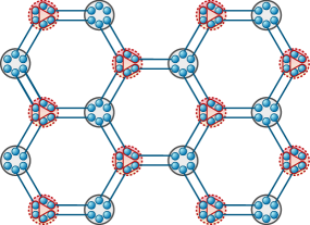
Honeycomb lattice with double bonds
Let us consider a honeycomb lattice where each pair of neighbouring nodes is connected by two copies of the same state ; see figure 9a. The CEP protocol converts all bonds shared by two parties into a single connection, and from majorization theory we know that a double bond can be optimally purified into one pair of qubits with entanglement . Setting this value to be equal to the percolation threshold for the honeycomb lattice, one finds that the entanglement can be propagated if , with
| (2.3tf) |
However, there exists another measurement pattern yielding a better percolation threshold (figure 9): half the nodes perform on their qubits three entanglement swappings, which maps the honeycomb lattice into a triangular one. Since the entanglement of the connections is not altered, on average, it follows that a lower threshold is found:
| (2.3tg) |
This proves that CEP is not optimal since it cannot generate long-distance entanglement in the range , whereas the quantum entanglement percolation achieves it with a strictly positive probability.
It is interesting to note that this example has also been used to show that the close analogy between quantum entanglement and classical secret correlations can be applied to entanglement percolation [76]. In this analogy, secret key bits, rather than entanglement are shared between neighbouring nodes.
3.2.3 Multi-partite entanglement percolation
We have seen that CEP can be enhanced by first applying some quantum operations at the nodes [23, 68, 71]. All examples proposed in these articles consist of transforming the quantum lattices by a sequence of entanglement swappings, thus conserving the average entanglement of the bonds. They are, however, restricted to purely geometrical transformations, and they apply to specific lattices only. In this respect, it was not clear whether the CEP strategy, and particularly the corresponding threshold, could be improved in general. A positive answer to this question was given in [77], in which a class of percolation strategies exploiting multi-partite entanglement was introduced. To that end, one performs the entanglement swappings in a more refined way, which we describe below.
Generalised entanglement swapping
The key ingredient of the multi-partite method is to consider a generalised entanglement swapping at the nodes: First, an incomplete measurement (i.e., not a complete projection) is performed at the central node by applying the operators
| (2.3th) |
for which the completeness relation is satisfied. This measurement leaves a two-dimensional subspace at the central station entangled with the two outer nodes. Thus, the central station still plays a role in the propagation of entanglement through the lattice. Second, not only two but links are “swapped” at the same time, and then the Procrustean method of entanglement concentration is performed on the resulting state; see (2.3o). These operations succeed with a finite probability that depends on the number of links and on their entanglement [77], generating the Greenberger-Horne-Zeilinger (GHZ) state
| (2.3ti) |
which is the generalisation of the Bell pair to qubits.
Entanglement thresholds: from bond to site percolation
In the multi-partite strategy one creates from the links of a quantum lattice a new lattice , where the nodes represent the GHZ states obtained with probability by the generalised entanglement swappings. Two vertices in are connected by a bond if the corresponding GHZ states share a common node in the original lattice. This defines a site percolation process with occupation probability , and above the site percolation threshold of the new lattice, the entanglement is propagated over a large distance as follows. Consider the situation in which two GHZ states of size and sharing one node have been created. One builds a larger GHZ state on particles with unit probability by performing a generalised entanglement swapping on the two qubits of the common node. This operation is iterated, eventually yielding a giant GHZ state spanning the lattice. Then, given a GHZ state of any size, a perfect Bell pair is created between any two of its qubits by measuring all other qubits in the basis.
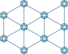
An example of multi-partite entanglement percolation is given in figure 10.
In this case, since the probability to create a
GHZ state of three qubits is equal to that of creating a
Bell pair (only two links are required), the minimum amount
of entanglement of the bonds for generating long-distance
entanglement is , which is equal to
the site percolation threshold in [78]. Since the critical value for CEP is (the threshold for bond percolation in [79]),
it follows that multi-partite entanglement percolation
surpasses CEP in the range .
The previous example appeared in [77] together with many other lattices for which the critical values using the multi-partite strategy are lower than the thresholds for CEP. In particular, an improvement is found for all Archimedean lattices, which are tilings of the plane by regular polygons (such as the square or the triangular lattice). Moreover, it is shown that not only the thresholds but also the probabilities are better for any amount of entanglement . This clearly indicates that the interplay of geometrical lattice transformations and multi-partite entanglement manipulations is a key ingredient for propagating entanglement in a quantum network.
3.3 Towards noisy quantum networks
We have already noted that creating perfectly entangled states via LOCC by consuming a finite number of states on a network of links of full-rank mixed states is not possible, even considering perfect operations. Two directions we may take from here are: i) If we cannot create a Bell pair, we may try to create a state with the highest possible fidelity. ii) Ask instead: For what class of mixed states it indeed possible to create a Bell pair, and what are the optimal protocols?
We have already paid some attention to the first question above and will review a more detailed examination in section 5.4. The answer to the second question is based on two results: i) It is not possible to transform a single copy of a mixed state to a pure state with local operations, and ii) In the case of two-qubit pairs, a pure state may only be obtained from two or more pairs belonging to a certain class of rank-two states [80], which we shall call purifyable mixed states (PMS). Protocols on networks using this approach were studied in [24, 25]. This work was extended to a hybrid approach addressing both the first and second question in [81]. The protocols presented in these three articles are the subject of this subsection. Note that what these authors call a PMS is a slightly more restricted class of states.
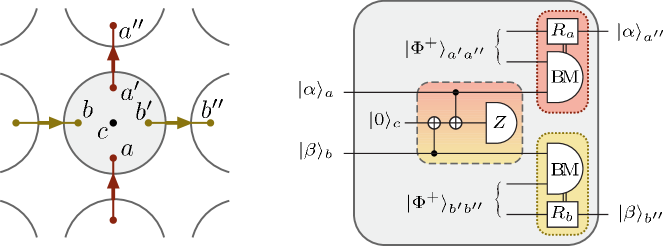
The most obvious constraint on the design of entanglement distribution protocols is that at least two disjoint paths of PMSs must exist between two stations in order to have a non-zero probability of a Bell pair between them. The final stage must consist of purifying multiple PMSs. We optimally convert two PMSs to a Bell pair in two stages. First, we perform a pure-state conversion measurement (PCM) as follows. We perform a quantum logic operation consisting of unitaries called the controlled-NOT gate at each local station, with qubits from one pair acting as targets in both cases. We then measure the targets in the computational basis, and if both results are , we have generated a pure state. If the two input states were identical, then the output state on success is already a Bell pair. But, in general, another Bell pair conversion using the Procrustean method according to (2.3o) in section 2.2.3 must be performed. However, as we shall see below, it is sometimes advantageous to delay this final Bell pair conversion and use the intermediate state in a different way.
Swapping
The behaviour of PMSs under swapping is similar to that of pure states. As in the case of pure states, we project onto the Bell basis, but now only two of the resulting states are useful, themselves being PMSs. Most importantly, the fidelity of the average resulting state decays exponentially in the number of links as it does for pure states.
CEP
CEP protocols analogous to pure state protocols are defined by taking regular lattices with multiple PMSs per bond. This is the most basic way to provide the necessary two pairs between nodes. This situation is similar to the double-bond honeycomb lattice of section 3.2.2, except that the states are PMSs and there may be more than two pairs connecting nodes. We saw for pure states that a Bell pair conversion on each bond succeeds with a probability , mapping the entanglement distribution problem to classical percolation with bond density . In the present case, we still map directly to classical percolation, but the bond density is determined by the success rate of some conversion protocol of the PMSs to a Bell pair. For two PMSs, the optimal protocol for this conversion is known [80] and has a maximum success rate , so that, for instance, percolation is possible on the double-bond triangular lattice but not on the double-bond square lattice. It is possible to achieve for three or more bonds, but the optimal conversion protocol is not known in this case. One protocol projects locally the entire state onto the subspace that is pure and entangled [82]. This was investigated in [25], along with better protocols that purify multiple bonds in smaller groups and reuse states from some of the failed conversions.
QEP
We have seen that for pure-state entanglement percolation, the first step in quantum pre-processing that goes beyond CEP is to note that, for a chain of two pairs, swapping before Bell pair conversion is better than Bell pair conversion before swapping. For PMSs the simplest analogy has more choices of when to do a pure-state conversion (PCM), Bell pair conversion, or swap, because we need a minimum of two pairs in parallel for each link in the chain. It turns out that the optimal method for this case of two pairs per link is to perform the PCM on each link and then to swap the resulting pure states before doing a Bell pair conversion. If the input states are identical, this is equivalent to CEP because, as mentioned already, a successful PCM already returns Bell pairs. In [25] this method was applied to small configurations and the results, in turn, to some regular and hierarchical lattices.
In all of these protocols, the only non-trivial case, with respect to CEP, is when the multiple pairs making up a link are PMSs with differing parameters; otherwise we get CEP again after the first purification step. In the case where the parameters are different within a link, we must first do a PCM, which maps the problem to the original pure-state percolation problem with some of the links probabilistically deleted. A similar idea is used in [81], where pairs in certain rank-three states replace the PMSs. These can be converted to binary states via a sort of PCM that leave a separable state on failure. The resulting lattice can be treated with error correction methods as in section 4, with the difference that the pairs in binary states are deleted probabilistically.
3.4 Open problems
It is natural to wonder about the optimality of the protocols based on entanglement percolation, either for pure states or for certain classes of mixed states. We focus on the square lattice here because it is very common, but the arguments apply to other lattices equally well.
It is obvious that percolation protocols cannot be optimal for every amount of entanglement of the links. In fact, we have seen in section 3.1.2 that a long-distance perfect Bell pair can be obtained deterministically if is larger than the threshold , whereas this is possible in entanglement percolation only if . On the other hand, the purification method completely fails if , while CEP yields positive results in the range . Consequently, considering one strategy only for all values of entanglement is not sufficient, but finding the optimum one for a given value in the links is a formidably difficult problem [68, 71, 77]. In this respect, multi-partite entanglement percolation is well-suited to generate long-distance quantum correlations regardless of the entanglement of the links, since it leads to high connection probabilities and low thresholds at the same time. A somewhat more tractable question is:
-
Does there exist a value of entanglement per link below which it is impossible to entangle two infinitely distant qubits using LOCC in a two-dimensional quantum network?
In the case of pure states the answer to this question is not known [54, 77]. Strategies based on multi-partite entanglement percolation are among the most efficient ones that achieve this task (see chapter 2.4 in [54] for a slight improvement of this scheme), but other efficient protocols may exist. For instance, it was shown in [26] that long-distance quantum correlations can be obtained in a square lattice using techniques of error correction (section 4.3.1).
Quite surprisingly, the situation turns out to be opposite in the case of mixed-state networks. In fact, suppose that the connections of the network are given by the Werner state , with smaller than the (classical) threshold for bond percolation in the corresponding lattice. That is, the quantum state describing the whole system is a classical mixture of lattices whose links are either perfect Bell pairs or completely separable states. In the limit of infinite size, however, none of these lattices possesses an infinite cluster of Bell pairs. The threshold is thus a lower bound on for a lattice of states since, by definition, no local quantum operation can create entanglement from separable states. In the square lattice, for instance, genuine quantum correlations cannot be generated over arbitrarily large distances if , even though all connections are entangled in the range . Finally, the situation for mixed-state lattices in three dimensions is similar to that of pure states: there exists a threshold to generate long-distance entanglement in the cubic lattice (section 4.3.3), but no interesting lower bound is known. In fact, the previous argument leads to a lower bound given by the percolation threshold on the cubic lattice [83], but at this bound the quantum connections are useless in any case since is separable for . The previous argument can be generalised to any mixed state using the concept of the best separable approximation (BSA) to an entangled state, introduced in [84]. Given a quantum state , one decomposes it as the mixture of an entangled and a separable state, and , with positive weights and such that :
| (2.3tj) |
The BSA to the state is defined by the decomposition maximising . Clearly, if the states in a network are such that the separable weight of its BSA is smaller than the network percolation threshold, there is no protocol allowing long-distance entanglement distribution.
In conclusion, it is of great interest to determine if there exists a lower bound for propagating the entanglement in quantum networks, and, if this is the case, to design new protocols that bring as close to as possible.
4 Network-based error-correction
In the previous section, we showed that percolation allows one to efficiently create entangled pairs of qubits over a large distance in quantum networks that consist of pure states or of a restricted class of mixed states. This is a considerable improvement over one-dimensional systems, in which the probability to generate remote entanglement decreases exponentially with the distance. The connectivity of the nodes plays a key role in this respect, but it is not clear if a similar effect exists in networks subject to general noise, that is, described by mixed states of full-rank. In fact, a finite number of such states cannot be purified into maximally entangled states (section 2.2.3), which is an essential requirement for entanglement percolation.
The aim of this section is to review the strategies that have been developed for propagating the entanglement in quantum networks whose connections are full-rank mixed states. However, we restrict our attention to Werner states defined in (2.3h). This entails little loss of generality because any mixed state can be transformed to a Werner state with the same fidelity via depolarisation.
4.1 A critical phenomenon in lattices
While most results on distribution of pure-state entanglement on lattices are based on percolation theory, another critical phenomenon lies at the heart of the propagation of mixed-state entanglement. Without being too rigorous, let us describe here this phenomenon in the case of a (classical) square lattice; the connection to quantum communication with mixed states is made in the next sections.
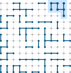
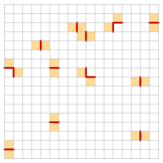
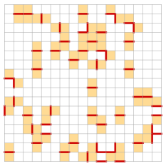
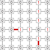
Links of the lattice are randomly set to “defective” with probability and to “valid” with probability , but we suppose that one cannot test a link to determine its validity. Instead, only a specific kind of information can be extracted from the lattice: for each square, or more generally for each vertex of the dual lattice111 In graph theory, the dual of a lattice is defined as follows: closed surfaces (polygons) in are mapped to vertices in , and two such vertices are connected if the corresponding polygons share an edge in . For example, the dual of the triangular lattice is the hexagonal lattice and the square lattice is self dual., we have access to the parity of adjacent links that are defective. Namely, vertices of the dual lattice get the value 0 if the number of such links is even and 1 otherwise. We call syndromes those vertices which are set to 1, since they indicate that defective links lie in their proximity. This fact is particularly obvious when is small, see figure 11a.
Given a pattern of syndromes, one shows that most defective links can be detected if is smaller than a critical value (figure 11 and section 4.2.3). In the remainder of this section, we describe how this phenomenon can be used to create long-range entanglement in mixed-state lattices.
4.2 Correction of local errors from a global syndrome pattern
At present, few schemes have been proposed to generate long-distance quantum correlations in noisy networks [26, 27, 28, 29, 30]. Although the quantum operations that are performed at the nodes are quite different for each scheme, the underlying principle is similar:
-
1.
The bonds are used to create a multi-partite entangled state that is shared by all nodes of the network. Due to the noise in the system, the generation of this state is imperfect;
-
2.
Local measurements on all but two distant qubits partially reveal at which places the noise altered the creation of the multi-partite state;
-
3.
A global analysis of the measurement outcomes determines the operations that have to be applied on the remaining two qubits in order to get useful remote entanglement.
These steps are described in more detail in what follows, and the schemes are reviewed in section 4.3.
4.2.1 Creation of a multi-partite entangled state
A first hint of the usefulness of multi-partite quantum states was given in section 3.2.3. In that setting, a giant GHZ state is created on the lattice by extracting perfect entanglement from the bonds adjoining each node. Then, measurements in the basis of all but two qubits transform the giant state into a Bell pair between the two remaining qubits. Finally, a local basis rotation depending on the measurement outcomes further converts the Bell pair into, say, the maximally entangled state . The procedure is rather similar here, but the links of the networks are used to create either a GHZ state (section 4.3.1), a surface code (section 4.3.2), or a cluster state (section 4.3.3). The key point of the construction is that while these states are simple enough to be created by local operations on the nodes of the quantum network, they also are tolerant of a certain amount noise, as described in the following sections.
4.2.2 Syndrome pattern
In the protocols involving pure states, it is known exactly whether a conversion of partially entangled states into Bell pairs succeeds or fails, since this information is given by the outcome of a measurement. In contrast, in mixed-state quantum networks, some noise enters the system randomly, and there is no way, a priori, to know where this happens. In fact, because every connection is a Werner state with non-unit fidelity, the generation of the multi-partite state based on such connections leads to a quantum state that contains errors (for instance, bit-flip and phase errors on some of its qubits). Hence, if one decides to measure all but the two target qubits right after the generation of the multi-partite state, then the choice of the final basis rotation will be correct with a probability of approximately only one fourth. This means that we have no knowledge at all about which one of the four Bell pairs we are dealing with, or in other words, the qubits are in a separable quantum state.
One strength of the network-based error correction is that one can gain some information about the errors without damaging the long-distance quantum correlations. In fact, the multi-partite entangled states created in the quantum network are highly symmetrical and satisfy a set of eigenvalue equations that can be checked by local measurements: if the outcomes do not match the symmetry of the target state at the corresponding nodes, which is called a syndrome, then one immediately knows that at least one adjacent link inserted an error into the system; see section 4.3. The question of determining which link is responsible for the syndrome is treated in what follows.
4.2.3 Error recovery
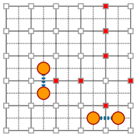
Syndromes are defined on the nodes of the dual lattice of the quantum network, which is either a square lattice (first two schemes) or a cubic lattice (third scheme). The generation of the multi-partite entangled state is such that the noise entering the system corrupts every link of the dual lattice with probability . This creates chains of errors, which are consecutive corrupted links of the dual lattice. Syndromes correspond to the endpoints of these chains and thus come in pairs, as depicted in figure 12a.
If one knew the location of all chains of errors, then it would be possible to perfectly restore the target multi-partite state. The difficulty of the error recovery is that while the positions of the syndromes are known, no other information about the chains is available. Since different chains of errors can lead to a similar syndrome pattern, the recovery is ambiguous and may lead to a wrong correction of the errors. However, Dennis et al. showed that, in an infinite square lattice, a (partial) recovery is possible if the error rate does not exceed a critical value [85]. This threshold is found via a mapping to the random-bond Ising model and is approximately equal to , which is numerically calculated in [86]. In order to obtain long-distance quantum correlations for , one should be able to compute all patterns of errors that lead to the measured syndromes and then to choose the one that most likely occurred. This is in-feasible in practice, but for small error rates , a good approximation of the optimal solution is the pattern in which the total number of errors is a minimum. In fact, such a pattern may be efficiently found by a classical algorithm, known as the minimum-weight perfect matching algorithm [87, 88]. Illustrations of these ideas are given in figure 12b and figure 12c.
4.3 Examples of protocols
Now that the general concepts about network-based error correction have been introduced, we describe in the following paragraphs the quantum operations that are required to generate entanglement over long distance in noisy networks, as proposed in [26, 27, 28].
4.3.1 Independent bit-flip and phase errors
Any entangled state of two qubits can be transformed by LOCC to the Werner state defined in (2.3h), but to understand the scheme of [26] it is more appropriate to consider a slightly different parameterization of a two-qubit entangled mixed state:
| (2.3ta) |
In this equation, and stand for the probability that the second qubit of the ideal connection has been affected by a bit-flip and a phase error, respectively. This state is as general as a Werner state in the sense that any quantum state of two qubits can be brought to this form using LOCC only.
Protocol in the case of bit-flip errors only
The links of a square lattice are used to create a giant GHZ state of qubits; see figure 2. For each direction, the stations perform the generalised entanglement swapping described in (2.3th). If one temporarily assumes that phase errors are not present in the links of the network, then the resulting multi-partite state is a mixture of GHZ states whose qubits are flipped with probability . If the error rate does not exceed the critical value , then most bit-flip errors can be corrected, as depicted in figure 14.
The bit-flip error correction presented above can be applied to arbitrary planar networks, as shown by Broadfoot et alin [81]. They also prove that it can be generalised to entangled mixed states of rank three, but another method has to be used in the case of full rank mixed states, which is the topic of the following paragraph.
Protocol including both bit-flip and phase errors
The global error correction works exactly as described above, but each qubit is replaced by a logical qubit which is an encoded block of qubits. Furthermore, all quantum operations on the logical qubit are implemented by an appropriate protocol at the encoded level. Phase errors are then suppressed by the redundancy of the following code:
| (2.3tb) |
where are the eigenvectors of the basis. Using majority vote, up to phase errors can be corrected for each block of qubits. A detailed discussion of a fault-tolerant implementation of this encoding is done in [26], but here it is sufficient to state the final result: long-distance quantum correlations can be obtained with the encoded version of the global bit-flip correction, but the number of links between neighbouring stations has to increase logarithmically with the distance. The main difference with the one-dimensional quantum repeaters is that all operations can be applied simultaneously, so that no quantum memory is needed.
4.3.2 Surface codes
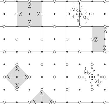
Surface codes have been used to implement error correction in quantum computation and communication [89, 90, 91, 92, 93, 94]. Here, we review three ways in which the surface code is used to generate entanglement over large distances. The protocol described in [27] differs from the previous protocols in that the data to be transmitted is encoded across the network as the multi-partite state is created. In [29], the authors propose to use the entanglement existing in the links of the network to apply stabiliser measurements and to create the surface code across the network. In both proposals the number of required entangled pairs scales with the distance at which the entanglement is to be generated. In what follows we describe these two protocols, whereas the third one, which requires a constant number of quantum connections only, is described in section 4.3.3.
Planar surface code
For the planar surface code, half of the qubits encode the data and half are only used to measure syndromes. The code is implemented via stabilisers. A stabiliser of is an operator satisfying . Data is encoded by preparing the array in a simultaneous eigenstate of a set of commuting stabilisers, which are defined as follows. A lattice is formed by associating an edge with each data qubit. Each face represents a stabiliser formed by the tensor product of four Pauli operators tensored with the identity on all other data qubits. Vertex stabilisers are defined similarly, substituting the operator for the operator. The exceptions are on the edges of the array, where the stabilisers are products of only three Pauli operators. The dimensions of the lattice are chosen to give two boundaries with partial vertex stabilisers, and two with partial face stabilisers, which ensures that the dimension of the space satisfying the stabiliser conditions is . That is, the array encodes one logical qubit. Details of surface codes and error correction can be found in [85].
Surface code communication protocol
The planar surface code is implemented on a two-dimensional rectangular array of entangled qubits and encodes a single logical qubit; see figure 15. We begin with a long rectangular array that supports this code. Square sections on the left and right ends also each support a surface code. The left end is prepared in a logical state and the right end in the logical state . A sequence of operations is performed in such a manner that it spreads the state until the entire array encodes . Finally, we perform some measurements that leave the array on the right end in the state . Errors are measured during the entire procedure and passed classically to the right end, where they are processed to correct the result.
Implementing the surface code communication protocol
The array is initialised with on the left and on the right, while all the data qubits in the middle are measured in the basis. The state is then spread across the array by measuring each stabiliser a number of times equal to code depth , which is the same as the height of the lattice. In general, increasing allows better correction for gate errors. The sequence of six gates shown in figure 15 is designed so that all stabilisers may be measured simultaneously. As a result of the repeated measurements, the syndromes mark chains of errors that extend in time (for discrete steps) as well as space. A change in a stabiliser measurement signals a syndrome marking the beginning or end of a chain. These error chains can be corrected in the same way as described in the previous subsection.
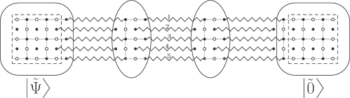
As it stands, this protocol creates and transports entanglement only through local interactions. Thus, it is not sufficient for communication between distant parties. For long distance communication, each syndrome qubit is replace by two syndrome qubits, each of which is coupled to one party of a Bell pair as shown in figure 16. The Bell pairs must be generated for each of the steps in spreading the surface code.
Assuming no loss in transmission and that all gates within the repeater nodes are perfect, the average time to failure of a single link only grows non negligibly with the code depth if the fidelity of the entangled pairs satisfies . Furthermore, the authors find that by modelling loss in transmission as measurement in an unknown basis, loss rates less than can be handled efficiently. They find that realistic gate error rates do not affect these results significantly. The number of qubits per repeater grows with the code depth , which scales as , where is the number of links and is the desired communication error rate. Reference [27] includes a more thorough discussion of the error rate and transmission rate.
Network-based surface code protocol
The authors of [29] suggest a different scheme to generate long-distance entanglement based on the surface code. The main idea is to use the entanglement present in the links of the network to perform stabiliser measurements on qubits sitting in different nodes. More specifically, the authors consider a square lattice where, besides the four qubits composing the network, each node has one extra qubit (called a processing qubit); see figure 17. The nodes are divided in three categories, black, red, and blue, in such a way that each red or blue node is surrounded by four black nodes. After initialising the processing qubits of black nodes in the state , the entanglement shared between neighbouring nodes is used to perform stabiliser measurements. According to the circuit depicted in figure 18, red nodes perform the stabiliser measurements , while blue nodes measure ( denotes the neighbours of red or blue nodes). If the entanglement shared in the network is perfect, that is, if the links are given by Bell states, the state of the black processing qubits after the stabiliser measurements is transformed into an eigenstate of the surface code. The last step of the protocol consists in measuring all black processing qubits except the ones that are held by Alice and Bob. The basis for these measurements is chosen to create a maximally entangled state between Alice and Bob.
Due to imperfections, however, errors in the entanglement shared in the network and in the operations result in incorrect stabiliser-measurement outcomes. In order to detect these errors, the stabiliser measurements are repeated times. For each measurement run, a new entangled pair of qubits must be generated between neighbouring sites. Since the desired state is an eigenstate of the stabiliser measurements, consecutive measurements with differing outcomes indicate an error. Finally, the errors are corrected by pairing the error syndromes through the network-based error correction.
The described protocol tolerates an error rate of approximately in the quantum channels composing the network, which, in turn, corresponds to links composed by Werner states with . One of the advantages of the scheme presented in [29] is that the same black processing qubit can be used to measure its four neighbouring qubits.
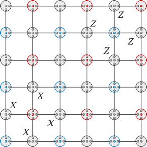
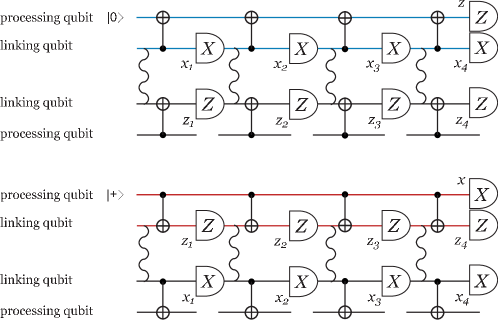
4.3.3 Entanglement distribution with constant resources
In the error-correction based protocols described above, the number of entangled pairs shared by neighbouring nodes has to increase with the size of the network in order to generate long-distance entanglement. On the contrary, it is shown in [28, 30] that a constant number of Werner states between neighbours is sufficient to achieve this task. In the following, we discuss the proposal of [28] which uses cluster states in a 3D lattice. We then briefly describe the main idea of [30], which works both for 2D and 3D lattices.
Three-dimensional cluster states
The first protocol achieving long-distance entanglement with a constant number of connections was proposed in [28]. In that article, it was shown that if the fidelity of the connections is larger than a critical value , then entanglement can be generated between two qubits and lying on opposite faces of a simple cubic lattice of size , with . In this case, however, it must be stressed that the local quantum operations are assumed to be perfect, which is not necessary for the other strategies that are fault-tolerant. In what follows, we describe in detail how this protocol works, but let us first define the cluster state, which lies at the heart of this proposal.
A cluster state is an instance of graph states [95], and it is usually constructed by inserting a qubit at each vertex of the graph and by applying a controlled-phase333Under a controlled-phase operation, the state is multiplied by , while , , and are unchanged. between all neighbours. This state obeys the eigenvalue equation for all vertices , where is the stabiliser
| (2.3tc) |
and where stands for the neighbourhood of in the graph. In [28], the desired controlled-phases are non-local quantum operations, and therefore they have to be performed indirectly through the use of the entangled connections and by applying some generalised measurements at the nodes. If one uses the noisy connections defined in (2.3ta), some errors are introduced into the system and the cluster state is not perfect anymore. Setting the bit-flip and phase error rates to , it can be shown that this results in local errors occurring independently at the nodes with a probability .
Three-dimensional cluster states are known to have an intrinsic capability of error correction. In fact, long-range entanglement was shown to be possible between two faces of an infinite noisy cubic cluster state [96]. The difference between [96] and [28] is that local quantum operations are assumed at every node in the latter case, in particular in the two faces. The error correction runs as follows. First, all qubits but and are measured in either the or the basis. The measurement pattern is such that, in the ideal case, the qubits and are maximally entangled:
| (2.3td) |
where the eigenvalues depend on the measurement outcomes and and are calculated from the stabiliser equations (2.3tc). The effect of the local errors is to change the sign of these eigenvalues, thus ruining the quantum correlations if no error recovery is performed. Then, the lattice is virtually divided into two interlocked cubic sublattices (one for each correlation and ), and a parity syndrome is assigned to nearly all vertices :
| (2.3te) |
where designates the neighbourhood in the corresponding sublattice. Since this equation arises from a product of stabilisers, we have that if no noise is present in the system. However, errors do not commute with measurements, and the construction is such that an error changes the sign of two syndromes that are neighbours in the other sublattice.
We are thus back to the error recovery described in section 4.2.3, with two differences nonetheless. First, of course, the lattice is three-dimensional and not planar. Second, some syndromes lying on the opposite faces cannot be assigned a value because of the specific measurement pattern, whereas all syndromes are known in the usual error correction. This results in imperfect quantum correlations, but the Monte Carlo simulations performed in [28] indicate that the distant qubits and are entangled as long as the error rate is smaller than the threshold .
Teleportation-based protocol
In [26] it is shown that the problem of transmitting entanglement in a two-dimensional network is equivalent to the problem of fault-tolerant quantum computation in a one-dimensional array of qubits restricted to next-neighbour gates. Let us discuss how it works. First, consider a square lattice in which we would like to create long-distance entanglement, and let us suppose for the moment that all links of the network are perfect. Consider one of the diagonal array of qubits of this lattice as a one-dimensional quantum computer at the initial time ; see figure 19a. By teleporting each qubit of the computer twice, first right and then above, the state of the computer is mapped to an upper-right diagonal array of qubits. The computer is now at time . If between to one has to implement a two-qubit gate between two neighbour qubits, one first teleports one of the qubits up and the other right; see figure 19b. In this way, they end up at the same location, where now the gate can be locally applied. Finally, each qubit is further teleported to the diagonal defining .
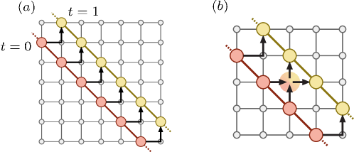
In the case that each link corresponds to a Werner state, the teleportation scheme can be seen as a quantum computation where errors occur. In this way, a fault-tolerant quantum computation scheme should be used. In fact, such a scheme exists, where two qubits per site are used [92]. Note that in fault-tolerant error-correction schemes, one starts by encoding a known state. However, in practice, in the very first stage the qubits are exposed to noise and thus decohere. Furthermore, in order to create an entangled state between two distant nodes, one would need a decoding scheme that is also fault-tolerant.
In reference [30] the authors develop a fault-tolerant encoding-decoding scheme into a 1D concatenated code [92] and into a 2D planar code [85] that works for unknown states. Both the encoding and decoding protocols can be done in a one-shot manner by measuring syndrome operators (products of and operators) and using error correction schemes based on syndrome patterns. By combining the encoding-decoding scheme in 1D or 2D, with the teleportation method shown in figure 19, one can establish long distance entanglement in the 2D and 3D square lattice network, respectively.
A simpler scheme of entanglement distribution in a 3D lattice was also discussed in [30], where the authors use a 2D topological code.
4.4 Conclusion
In this chapter, we have seen that long-distance entanglement can be generated in mixed-state networks. To this end, some information about where the noise (bit-flip and phase errors) enters the system must be collected. This is done by computing a series of parity checks at the nodes, which creates a syndrome pattern. Then, the errors are corrected by applying local unitaries that are determined by pairing, in an optimal way, the detected syndromes. Note that all proposed protocols are based on theoretical results for lattices of infinite size, so that it would be interesting, if not necessary, to investigate their efficiency for realistic networks of small or medium size.
5 Networks with a complex structure
Up to this point, we have seen protocols that generate entanglement over a large distance in quantum networks with a regular structure. In fact, as motivated in the Introduction, the creation of remote entangled qubits is of primary importance in quantum cryptography. To date, real quantum networks have been designed in a top-down, or executive fashion. But, as quantum information technology progresses, we will eventually see networks in which nodes and connections are added according to decisions that are taken locally, rather than purely by executive design. Such a process gives rise to self-organisation and complexity, with the internet being the most relevant example. In general, local organising principles give rise to complex networks. These networks describe a wide variety of systems in nature and society modelling, among other things, chemical reactions in a cell, the spreading of diseases in populations. We refer the reader to several books and reviews on this complex networks [97, 11, 9, 98, 99, 100]. In the following, we first introduce the random graph model in the context of complex networks. Then we review several studies of distribution and concentration of entanglement on complex networks.
The simplest model that manifests some features of complex networks was introduced by Rapoport [101, 102], and was treated in depth and rigorously by Erdős and Rényi [103, 104, 105]. In this model, known as the random graph, or Erdős Rényi (ER) model, each pair of vertices in a graph is connected by an edge with probability .
Although a great deal is known about the random graph, it lacks some of the important features of real-life complex networks. However, it is useful as a starting point, not only because it is easier to analyse, but because it exhibits at least two of the most important features of complex networks: 1) It possesses the small-world property, which means that the length of the shortest path between two nodes increases slowly with the system size. 2) It exhibits critical phenomena, with a critical point and a single cluster with macroscopic density. A quantum version of the random graph was proposed in [31], where it is shown that its properties change completely when they are subject to the laws of quantum physics (section 5.1).
Many measures have been suggested to quantify the main properties of real complex networks, but three concepts seem to occupy a prominent place [9]: the small-world [106], clustering [8], and scale-free [107] behaviours. A graph with the small world property typically has shortest paths between nodes that scale like , where is the number of nodes. Graphs with the small-world property may or may not have properties such as community structure or some regularity. But they have some links, perhaps a small fraction, that connect random nodes, or distant nodes if there is community structure. A graph with a large clustering coefficient has the property that, if is connected to both and , then it is likely that is also connected to . A scale free graph has the property that the probability that a node has links decays as a power of . While the ER graph satisfies the small-world property, it is not scale-free and has zero clustering coefficient. Many mathematical models have been introduced over the years to include the two other characteristics. However, in all of these networks, as in lattices, the method of entanglement percolation is applicable and the percolation thresholds are enhanced by some quantum strategies [108]; see section 5.3. In the following section, we treat yet another, but related, critical phenomenon: the appearance of connected structures of a given shape in a random graph.
5.1 Random graphs
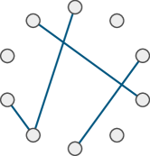
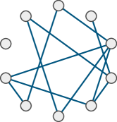
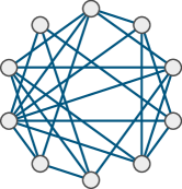
Here, we briefly introduce random graph theory; the interested reader is referred to [9] (and references therein) for a more detailed description of these graphs and a rigorous discussion of their properties.
The theory of random graphs considers graphs in which each pair of nodes and is joined by a link with probability . In the simplest and most studied model, the probability is independent of the nodes with . The generated graph is denoted and can considered to be the result of an evolution process: starting from isolated nodes, random edges are successively added with probability and the obtained graphs correspond to a larger and larger connection probability; see figure 20.
5.1.1 Appearance of subgraphs
One of the main goals of random-graph theory is to determine the probability at which a specific property of a graph typically arises, as tends to infinity. For fixed , the typical node-degree diverges with , leading to a highly-connected, boring graph. Instead, we let , with details of the dependence allowing us to examine different interesting phenomena.
Many properties of interest appear suddenly, i.e., there exists a critical probability such that almost every graph has this property if and fails to have it otherwise. Such graphs are said to be typical. For instance, it was shown that is fragmented into small isolated clusters if , whereas percolation occurs above this threshold, that is, one single giant component forms in the network.
A subgraph of is defined as a collection of vertices connected by edges. Like the giant cluster, the subgraphs have distinct thresholds at which they typically form. It is proven in [109] that the critical probability for the emergence of is
| (2.3ta) |
where is independent of . It is instructive to look at the appearance of subgraphs assuming that scales as , with a tunable parameter: as increases, more and more complex subgraphs appear; see table 1. In particular, only node-to-node connections appear in the regime , whereas complete subgraphs (of order four or more) emerge above the percolation threshold .
|
|
|
|
|
|
5.2 Quantum random graphs
A natural extension of the previous scenario to a quantum context was considered in [31]. For each pair of nodes, the probability is replaced by a quantum state of two qubits, one at each node. Hence, every node possesses qubits that are pairwise entangled with the qubits of the other nodes. The study is restricted to the pure-state scenario and the pairs of particles are identically connected, so that . A quantum random graph is then defined as
| (2.3tb) |
Expanding all terms of this expression in the computational basis, one notes that this state is the coherent superposition of all possible simple graphs on nodes, weighted by the number of states they possess. For instance, drawing a line for the state 111Note that, contrary to the rest of the Review, a line denotes here a separable state rather than entangled qubits. and nothing for , the quantum random graph on three nodes reads:
| (2.3tc) |
The analogy with the ER model is that one lets the degree of entanglement of the connections scale with the number of nodes: . In this case, the “classical” strategy is to optimally convert each connection of the graph, individually, into the Bell pair , as described in section 2.2.3. The task of determining the type of maximally entangled states remaining after these conversions is mapped to the classical problem, and one obtains again the results of table 1 with .
5.2.1 A complete collapse of the critical exponents
The main result in [31] states that, in an infinitely large quantum random graph and in the regime , the state
| (2.3td) |
which corresponds to any subgraph composed of vertices and edges, can be generated with a strictly positive probability using LOCC only. All critical exponents of table 1 thus collapse onto the smallest non-trivial value . This clearly indicates that the properties of disordered graphs change completely when they are governed by the laws of quantum physics. It is not the purpose of this Review to prove this result, but let us describe the main quantum operation that lies behind its proof. In fact, it is another example of a generalised measurement on many qubits that enhances the distribution of entanglement in quantum networks.
A joint measurement at the nodes
As for multipartite entanglement percolation (section 3.2.3), allowing strategies that entangle the qubits within the nodes yields better results than a simple conversion of the links into Bell pairs. In the current case, the construction of a quantum subgraph is based on an incomplete measurement of all qubits at each node. More precisely, the measurement operators are projectors onto the subspaces that consist of exactly states out of qubits:
| (2.3te) |
where denotes a permutation of the qubits. Applied on all nodes of the quantum random graph, this measurement generates a highly entangled state shared by a random subset of nodes. The quantum correlations corresponding to are then extracted by a suitable series of local operations at these nodes [31]. Note that this measurement allows not only the creation of any quantum subgraph, but also the generation of some important multipartite states, such as the GHZ states [54].
5.3 Percolation
One may ask what pure-state entanglement percolation looks like on complex networks rather than regular lattices. It is obvious that CEP on complex networks works exactly as it does on regular lattices; but it is not obvious how to design pre-processing for QEP. However, a particular QEP protocol has been applied with success to a variety of complex networks with double-bond, pure, partially-entangled states [108, 110]. As in the many cases of links with multiple pairs that we have seen, this setup makes possible the systematic application of a simple local transformation, with the hope that general global effects can be understood.
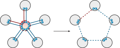
Following [110], we consider here networks where each link between nodes consists of two pairs in the state ; see (2.3e). CEP consists of the optimal conversion of each pair of pairs to a Bell pair, followed by swapping. The QEP protocol consists of optionally performing swaps at a node of degree , with even. The swaps join pairs of links terminating at the node. Thus, the node is replaced by a cycle whose bonds are occupied with states according to the random outcome of the swapping; see figure 21. We call the original node and its bonds a -star, the transformed object a -cycle, and the transformation a -swap. Whether it is advantageous to apply the -swap depends on the details of the network.
The interesting parameter regime for complex networks is often the tree-like regime– that is, when there are so few links that the probability that there is more than one path connecting two nodes is negligible. For instance, the percolation transition of the ER network is in the tree-like regime. The usual way to analyse tree-like networks is with generating functions and recursion, which gives exact results in this limit. Although the -swap creates loops, they are small and isolated, so that an entire -cycle can be treated at one step in the recursion. Still, one has a choice in applying -swap because, for instance, it cannot be applied at neighbouring nodes. In [110] this calculation was done for a breadth-first application, that is, applying the -swap at neighbour of a starting node, and then at next-nearest neighbour’s, where possible, etc. Exact results were obtained for various networks. For instance, it was shown that any application of -swap on a tree lowers the threshold with respect to CEP; see section 3.1.1. The generating-function analysis shows that, in the tree-like regime, the optimal strategy with node-degree is to either always or never perform -swap depending on the lattice and . For other lattices this fact comes into play. For example, on the ER network, the optimal application of -swap yields the best results for average degree near with a 20% reduction in the threshold, with similar results for the un-correlated scale-free network.
The presence of small cycles is recognised as a key feature of many complex networks. In a network of scientific collaborators, for instance, one can identify small groups, each member of which has been a coauthor with each of the others. Of course, this phenomenon cannot be modelled in the strict tree-like limit. Thus other models and techniques of analysis, largely numeric, are required. For instance, the Watts-Strogatz model begins with a one-dimensional chain of nodes connected with nearest-neighbour’s and next-nearest-neighbour connections. The terminal node of each bond is then randomly rewired with small probability . The original local connections give the model community structure, while the rewired bonds provide a few long-range links that drastically reduce the shortest path between nodes. Numerical simulations showed less impressive improvements than the tree-like models. Still, the critical threshold is lowered by -swapping. However, this form of QEP is not always advantageous. For large enough initial entanglement per link, the CEP produces a Bell pair with probability and the giant connected component is larger for CEP than for -swap.
5.4 Mixed state distribution
Here we discuss distributing full-rank mixed states on complex networks. One approach is to admit that the exponential decay of entanglement due to swapping imposes an upper limit on the number swaps that may be performed, before all entanglement is lost. The distance corresponding to this limit can be included in calculations of statistical properties of entanglement. For instance, if this limit is smaller than the correlation length, then the network is essentially fractured with respect to entanglement via direct swapping. This approach was taken numerically and with generating functions in [110]. On the other hand, it is a priori possible to approximate maximally entangled links between distant nodes by concentrating links from ever larger numbers of paths. Studies to date have examined possible building blocks to this end [111]. This work quantifies the gain in concurrence obtained between nodes by employing concentration and distribution protocols on multiple paths. The most detailed results were obtained for the simplest case of the single purification protocol (SPP), in which the shortest path between and is identified, and then a shortest path between two nodes on is found. Both paths can be used to achieve a final entanglement between and that is larger than that achieved by using only; see figure 22.
In particular, we examine here the results of the SPP protocol applied to the ER random graph [111]. The initial network is the same as in the previous section, except that the links are Werner states (2.3h) rather than pure states. As mentioned above, it is impossible to extract a pure state from a finite number of Werner states. We instead search for a protocol that produces the mostly highly entangled mixed states possible. More specifically, we seek to maximise the average of the concurrence (2.3k),
| (2.3tf) |
where the sum is over all pairs of nodes in the network, is the probability that the protocol connecting and was successful and is the resulting concurrence between the pair.
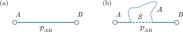
The most naive method to entangle two nodes and is to perform entanglement swapping repeatedly between Werner states along the shortest path joining and according to (2.3r); see figure 22a. However, in some cases, higher entanglement may be obtained by additionally concentrating the entanglement from an alternate path connecting intermediate nodes on the path as shown in figure 22b. In this single-purification protocol, one swaps along the subpath as well as the shortest available alternate path , then performs a purification on the two resulting parallel states, and finally performs swapping at all remaining links. Whether a higher entanglement results on average than that from simply swapping along depends on the lengths of the paths and the Werner parameter .

For instance, consider the parameters , , , and . A detailed analysis of the region in this parameter space for which this purification protocol yields a higher average concurrence is given in [111], and is shown graphically in figure 23.
Of course a network may offer more possibilities than concentrating the entanglement from a single neighbouring path. One could repeatedly concentrate entanglement from paths in parallel or series. Let us consider the latter case, where instead of a pair of paths and , we have pairs and that together the paths cover a fraction of . For simplicity we take . The region in parameter space for which this protocol is advantageous were computed exactly and are shown in figure 24. One sees that many short paths are better than few long paths, but that the maximum extent of the good region approaches a limit as .

Suppose we apply only the single-purification protocol at every possibility on a network. Computing the average concurrence over a random network is in general difficult. However, the ER network at its critical point is in the tree-like regime and has further statistical properties that facilitate calculations. In particular, the exact asymptotic increase in concurrence over the naive swapping protocol as a function of Werner parameter and number of nodes was found to be . Here is a constant that is easily computed by numerical integration. Although this expression diverges as , this occurs outside the asymptotic regime where the purified paths have lengths much shorter than the radius of the giant cluster.
It is important to note here that the above protocol is not capable of entangling arbitrarily distant nodes independently of the initial concurrence per link, but it is one that can be applied in principle to arbitrary networks.
The preceding protocols, although treating mixed states, have assumed perfect operations. If we further assume the noise model described in (2.3tu) and (LABEL:eq:noisy_measurement) we find that the protocol is rather sensitive to noise. The results are quantitatively similar to [6] with the advantage destroyed for noise levels larger than a few percent. For instance, the maximum average concurrence gain from the single purification protocol was found to be
| (2.3tg) |
where and .
The richer variety and topologies of complex networks provide a fertile terrain for developing more sophisticated distribution protocols. The studies reviewed here make only the first steps. In particular, they apply relatively simple quantum procedures for which averages over quantum outcomes and classical disorder may be performed. Other important directions remain completely unexplored, such as the dynamic creation and distribution of entanglement.
5.5 Optimal path for distributing entanglement on networks
Here we consider mapping entanglement distribution problems to classical graph algorithms. The majority of efficient classical algorithms for solving various shortest-path problems on graphs assume that the measure of path length is the sum of edge weights. This includes measures given by the product of non-negative edge weights, which are mapped to this additive class by considering the logarithm of the weights. A few of these shortest-path problems are: 1) shortest path between two nodes; 2) shortest paths between one node and all other nodes; 3) problem 1) or 2) restricted to positive edge weights. The key reason that many problems using these measures admit efficient algorithms is that they possess optimal substructure (also referred to as Bellman’s optimality principle): In this context, if is a node on the shortest path from to , then the later is composed of the shortest path from to and the shortest path from to . These topics have been researched and applied intensively and broadly for several decades. References [112] and [113] are two of the most popular textbooks treating the subject.
It is therefore of interest to know which entanglement distribution problems can be expressed as a classical shortest-path problem. For instance, suppose that each link is initially in a Werner state , with the parameter depending on . Then, using (2.3r), we see that the entanglement obtained by performing swapping at all nodes along a path becomes a path length if the weights are taken to be . Then, the path that yields the maximum entanglement between nodes and via a series of swaps is the shortest path between the nodes.
Another example is the question: Given the task of performing a series of teleportations on a network to transfer a state from node to node , may we efficiently choose the optimal path? In reference [114], the question is addressed using the following model. Assume the state to be transferred has the form (2.1), with the restriction ; That is 222In this case the restriction is significant, as we shall consider an average over these states.. The links are initially the partially entangled pure states described by (2.3e), but with Schmidt coefficients depending on the link index . The protocol consists of teleporting a state from to a neighbouring node, and then teleporting from this node to yet another, and so on, until the state arrives at . Before continuing, we make a brief digression into classification of protocols. All protocols involving pure states that we reviewed thus far are so-called probabilistic protocols; they involve recording a measurement and thus retaining information about the resulting state, which is one of a number of possible states, each obtained with a certain probability. Another kind of protocol, called a deterministic protocol, is used in the present scenario. In this case we don’t record the measurement, so that the output state is a mixture of a number of possible outcomes. Thus, even with a pure initial state and pure link states, and perfect operations, this results with probability one (i.e deterministically) in a mixed state . A measure of how close the state received at node is to the initial state at node is the fidelity . Choosing a particular path of links , and averaging this fidelity over all initial states, that is all allowed values of and , gives . Because each factor in the product can be associated with a link weight, this problem is amenable to efficient algorithms.
Reference [114] next generalises the problem slightly to the case that the initial state of each link is one of a class of mixed states that includes Werner states. In this case, it turns out that each link must be assigned two independent link weights and that depend on the parameters of the link state. Furthermore, the average fidelity now has the form
| (2.3th) |
Consider adding a single node that is connected to the network only by one link to node and using (2.3th) to compute shortest paths. It is easy to see that in general, the shortest path from to does not include the shortest path from to . Thus, the problem no longer possesses optimal substructure and cannot be solved by efficient algorithms that rely on this property.
Similar questions arise in classical network engineering, and in particular to their application to quantum networks. In general, one might hope to find a measure of path length that one hand satisfies the optimality principle, and on the other, whose minimisation is a reasonable approximation of a more difficult global optimisation problem. For instance, reference [115] studies a model optical network that creates and distributes Bell pairs via simulations depending on many of parameters. The authors compare optimisation based on various measures of the work done per link to the global throughput. The simulations show that, within this model, one can usually predict the path that simultaneously gives highest throughput, and, by some measure of operations, the lowest work.
6 Conclusion
In this review we have given an account of theoretical progress on the distribution of entanglement in quantum networks. We have seen that this inquiry has been driven by the experimental results on the building blocks of entanglement distribution. These results are impressive and promising, but also make evident fundamental and technical barriers. We have also seen that the task of distribution is intimately connected with theoretical questions about the nature of entanglement. In this setting, these questions are focused on the extent to which it can be measured and inter-converted. While the basic concepts (direct transmission, swapping, purification, error correction) have been present for over twenty years, their application to real networks is still in an exploratory phase.
The firsts steps to transmission of entanglement embodied in a variety of physical systems have already been taken. In fact, the most important application to date, the distribution of quantum cryptographic keys, has been demonstrated. Teleportation, as well, has been demonstrated in several systems. But the problem of exponential decay of fidelity has not been solved. Methods using the geometry of higher-dimensional networks to effectively concentrate entanglement from some sections for use in others shows promise in overcoming this difficulty. At the same time, they show strong connections with the theory of classical networks and graphs, in particular with percolation theory. Classical error correction also has proven to be useful in this regard, with interesting quantum connections, such as defining syndromes via weak measurements that preserve information.
It is clear that the study of entanglement distribution on mixed-state networks will be of prime importance. For instance, quantum cryptography will continue to be one of the main technologies driving research. Quantum repeaters are expected to become more robust, thereby allowing small networks to form. This will require new protocols adapted to these small networks. Eventually, we expect to see application of pioneering work in entanglement percolation and error correction. Finally, as the number of nodes increases to the point that statistical methods can be applied, we expect to see vigorous activity in the theory of complex quantum networks.
References
References
- [1] A. Einstein, B. Podolsky, and N. Rosen. Can quantum-mechanical description of physical reality be considered complete? Phys. Rev., 47(10):777–780, May 1935.
- [2] E. Schrödinger. Die gegenwärtige Situation in der Quantenmechanik. Naturwissenschaften, 23:807–812; 823–828; 844–849, 1935.
- [3] E. Schrödinger. Discussion of probability relations between separated systems. Mathematical Proceedings of the Cambridge Philosophical Society, 31:555–563, 1935.
- [4] J. S. Bell. On the Einstein-Podolsky-Rosen paradox. Physics, 1(3):195–200, 1964.
- [5] H. J. Briegel, W. Dür, J. I. Cirac, and P. Zoller. Quantum repeaters: The role of imperfect local operations in quantum communication. Phys. Rev. Lett., 81(26):5932–5935, Dec 1998.
- [6] W. Dür, H. J. Briegel, J. I. Cirac, and P. Zoller. Quantum repeaters based on entanglement purification. Phys. Rev. A, 59(1):169–181, Jan 1999.
- [7] L. Childress, J. M. Taylor, A. S. Sørensen, and M. D. Lukin. Fault-tolerant quantum repeaters with minimal physical resources and implementations based on single-photon emitters. Phys. Rev. A, 72(5):052330, Nov 2005.
- [8] D. J. Watts and S. H. Strogatz. Collective dynamics of small-world networks. Nature, 393:440–442, Jun 1998.
- [9] R. Albert and A.-L. Barabási. Statistical mechanics of complex networks. Rev. Mod. Phys., 74(1):47–97, Jan 2002.
- [10] D. J. Watts. Small worlds: the dynamics of networks between order and randomness. Princeton Univ. Press, 2004.
- [11] M. Newman, A.-L. Barabási, and D. J. Watts. The structure and dynamics of networks. Princeton Univ. Press, 2006.
- [12] H. J. Kimble. The quantum internet. Nature, 453:1023–1030, 2008.
- [13] W. K. Wootters and W. H. Zurek. A single quantum cannot be cloned. Nature, 299:802–803, Oct 1982.
- [14] M. A. Nielsen and I. L. Chuang. Quantum Computation and Quantum Information. Cambridge University Press, 2000.
- [15] R. Horodecki, P. Horodecki, M. Horodecki, and K. Horodecki. Quantum entanglement. Rev. Mod. Phys., 81:865–942, Jun 2009.
- [16] C. H. Bennett, G. Brassard, C. Crépeau, R. Jozsa, A. Peres, and W. K. Wootters. Teleporting an unknown quantum state via dual classical and Einstein-Podolsky-Rosen channels. Phys. Rev. Lett., 70(13):1895–1899, Mar 1993.
- [17] J. I. Cirac, A. K. Ekert, S. F. Huelga, and C. Macchiavello. Distributed quantum computation over noisy channels. Phys. Rev. A, 59(6):4249–4254, Jun 1999.
- [18] A. K. Ekert. Quantum cryptography based on Bell’s theorem. Phys. Rev. Lett., 67(6):661–663, Aug 1991.
- [19] Valerio Scarani, Helle Bechmann-Pasquinucci, Nicolas J. Cerf, Miloslav Dušek, Norbert Lütkenhaus, and Momtchil Peev. The security of practical quantum key distribution. Rev. Mod. Phys., 81:1301–1350, Sep 2009.
- [20] C. H. Bennett and G. Brassard. Quantum cryptography: Public key distribution and coin tossing. In Proceedings of IEEE International Conference on Computers, Systems and Signal Processing, pages 175–179, New York, 1984.
- [21] C. H. Bennett and S. J. Wiesner. Communication via one- and two-particle operators on Einstein-Podolsky-Rosen states. Phys. Rev. Lett., 69(20):2881–2884, Nov 1992.
- [22] C. Simon, M. Afzelius, J. Appel, A. Boyer de la Giroday, S. J. Dewhurst, N. Gisin, C. Y. Hu, F. Jelezko, S. Kröll, J. H. Müller, J. Nunn, E. S. Polzik, J. G. Rarity, H. De Riedmatten, W. Rosenfeld, A. J. Shields, N. Sköld, R. M. Stevenson, R. Thew, I. A. Walmsley, M. C. Weber, H. Weinfurter, J. Wrachtrup, and R. J. Young. Quantum memories. Eur. Phys. J. D, 58(1):1–22, 2010.
- [23] A. Acín, J. I. Cirac, and M. Lewenstein. Entanglement percolation in quantum networks. Nature Phys., 3(4):256–259, Feb 2007.
- [24] S. Broadfoot, U. Dorner, and D. Jaksch. Entanglement percolation with bipartite mixed states. Europhys. Lett., 88(5):50002, Dec 2009.
- [25] S. Broadfoot, U. Dorner, and D. Jaksch. Singlet generation in mixed-state quantum networks. Phys. Rev. A, 81(4):042316, Apr 2010.
- [26] S. Perseguers, L. Jiang, N. Schuch, F. Verstraete, M. D. Lukin, J. I. Cirac, and K. G. H. Vollbrecht. One-shot entanglement generation over long distances in noisy quantum networks. Phys. Rev. A, 78(6):062324, Dec 2008.
- [27] A. G. Fowler, D. S. Wang, C. D. Hill, T. D. Ladd, R. Van Meter, and L. C. L. Hollenberg. Surface code quantum communication. Phys. Rev. Lett., 104(18):180503, May 2010.
- [28] S. Perseguers. Fidelity threshold for long-range entanglement in quantum networks. Phys. Rev. A, 81(1):012310, Jan 2010.
- [29] Y. Li, D. Cavalcanti, and L. Kwek. Long-distance entanglement generation with scalable and robust two-dimensional quantum networ. Phys. Rev. A, 85(26):062330, June 2012.
- [30] A. Grudka, M. Horodecki, P. Horodecki, P. Mazurek, L. Pankowski, and A. Przysiezna. Long distance quantum communication over noisy networks, 2012. eprint arXiv:1202.1016.
- [31] S. Perseguers, M. Lewenstein, A. Acín, and J. I. Cirac. Quantum random networks. Nature Phys., 6:539–543, May 2010.
- [32] A. Peres. Quantum Theory: Concepts and Methods. Springer, 1995.
- [33] R. F. Werner. Quantum states with Einstein-Podolsky-Rosen correlations admitting a hidden-variable model. Phys. Rev. A, 40(8):4277–4281, Oct 1989.
- [34] G. Vidal. Entanglement of pure states for a single copy. Phys. Rev. Lett., 83(5):1046–1049, Aug 1999.
- [35] C. H. Bennett, D. P. DiVincenzo, J. A. Smolin, and W. K. Wootters. Mixed-state entanglement and quantum error correction. Phys. Rev. A, 54(5):3824–3851, Nov 1996.
- [36] W. K. Wootters. Entanglement of formation of an arbitrary state of two qubits. Phys. Rev. Lett., 80(10):2245–2248, Mar 1998.
- [37] C. H. Bennett, G. Brassard, S. Popescu, B. Schumacher, J. A. Smolin, and W. K. Wootters. Purification of noisy entanglement and faithful teleportation via noisy channels. Phys. Rev. Lett., 76(5):722–725, Jan 1996.
- [38] MB Plenio and S Virmani. An introduction to entanglement measures. Quantum Information and Computation, 7(1):001–051, 2007. eprint arXiv:quant-ph/0504163.
- [39] A. C. Doherty, P. A. Parrilo, and F. M. Spedalieri. Complete family of separability criteria. Phys. Rev. A, 69:022308, Feb 2004.
- [40] H. Hübel, M. R. Vanner, T. Lederer, B. Blauensteiner, T. Lorünser, A. Poppe, and A. Zeilinger. High-fidelity transmission of polarization encoded qubits from an entangled source over 100 km of fiber. Opt. Express, 15(12):7853–7862, Jun 2007.
- [41] N. Sangouard, C. Simon, H. de Riedmatten, and N. Gisin. Quantum repeaters based on atomic ensembles and linear optics. Rev. Mod. Phys., 83:33–80, Mar 2011.
- [42] M. A. Nielsen. Conditions for a class of entanglement transformations. Phys. Rev. Lett., 83(2):436–439, Jul 1999.
- [43] M. A. Nielsen and G. Vidal. Majorization and the interconversion of bipartite systems. Quant. Inf. Comput., 1(1):76–93, Jul 2001.
- [44] C. H. Bennett, H. J. Bernstein, S. Popescu, and B. Schumacher. Concentrating partial entanglement by local operations. Phys. Rev. A, 53(4):2046–2052, Apr 1996.
- [45] W. Dür and H. J. Briegel. Entanglement purification and quantum error correction. Rep. Prog. Phys., 70(8):1381–1424, Aug 2007.
- [46] N. Linden, S. Massar, and S. Popescu. Purifying noisy entanglement requires collective measurements. Phys. Rev. Lett., 81(15):3279–3282, Oct 1998.
- [47] A. Kent. Entangled mixed states and local purification. Phys. Rev. Lett., 81(14):2839–2841, Oct 1998.
- [48] D. Deutsch, A. Ekert, R. Jozsa, C. Macchiavello, S. Popescu, and A. Sanpera. Quantum privacy amplification and the security of quantum cryptography over noisy channels. Phys. Rev. Lett., 77(13):2818–2821, Sep 1996.
- [49] J.-W. Pan, S. Gasparoni, R. Ursin, G. Weihs, and A. Zeilinger. Experimental entanglement purification of arbitrary unknown states. Nature, 423:417–422, May 2003.
- [50] D. Bouwmeester, J.-W. Pan, K. Mattle, M. Eibl, H. Weinfurter, and A. Zeilinger. Experimental quantum teleportation. Nature, 390(6660):575–579, Dec 1997.
- [51] M. Żukowski, A. Zeilinger, M. A. Horne, and A. K. Ekert. “Event-ready-detectors” Bell experiment via entanglement swapping. Phys. Rev. Lett., 71(26):4287–4290, Dec 1993.
- [52] S. Bose, V. Vedral, and P. L. Knight. Multiparticle generalization of entanglement swapping. Phys. Rev. A, 57(2):822–829, Feb 1998.
- [53] S. Bose, V. Vedral, and P. L. Knight. Purification via entanglement swapping and conserved entanglement. Phys. Rev. A, 60(1):194–197, Jul 1999.
- [54] S. Perseguers. Entanglement Distribution in Quantum Networks. PhD thesis, Technische Universität München, 2010. Published by SVH Verlag, ISBN 3838118057.
- [55] J. I. Cirac, P. Zoller, H. J. Kimble, and H. Mabuchi. Quantum state transfer and entanglement distribution among distant nodes in a quantum network. Phys. Rev. Lett., 78(16):3221–3224, Apr 1997.
- [56] L. Hartmann, B. Kraus, H. J. Briegel, and W. Dür. Role of memory errors in quantum repeaters. Phys. Rev. A, 75(3):032310, Mar 2007.
- [57] D. Boschi, S. Branca, F. De Martini, L. Hardy, and S. Popescu. Experimental realization of teleporting an unknown pure quantum state via dual classical and einstein-podolsky-rosen channels. Phys. Rev. Lett., 80:1121–1125, Feb 1998.
- [58] A. Furusawa, J. L. Sorensen, S. L. Braunstein, C. A. Fuchs, H. J. Kimble, and E. S. Polzik. Unconditional quantum teleportation. Science, 282(5389):706, 1998.
- [59] Xiao-Song Ma, Thomas Herbst, Thomas Scheidl, Daqing Wang, Sebastian Kropatschek, William Naylor, Bernhard Wittmann, Alexandra Mech, Johannes Kofler, Elena Anisimova, Vadim Makarov, Thomas Jennewein, Rupert Ursin, and Anton Zeilinger. Quantum teleportation over 143 kilometres using active feed-forward. Nature, 489(7415):269–273, Sep 2012.
- [60] Juan Yin, Ji-Gang Ren, He Lu, Yuan Cao, Hai-Lin Yong, Yu-Ping Wu, Chang Liu, Sheng-Kai Liao, Fei Zhou, Yan Jiang, Xin-Dong Cai, Ping Xu, Ge-Sheng Pan, Jian-Jun Jia, Yong-Mei Huang, Hao Yin, Jian-Yu Wang, Yu-Ao Chen, Cheng-Zhi Peng, and Jian-Wei Pan. Quantum teleportation and entanglement distribution over 100-kilometre free-space channels. Nature, 488(7410):185–188, Aug 2012.
- [61] I. Marcikic, H. de Riedmatten, W. Tittel, H. Zbinden, and N. Gisin. Long-distance teleportation of qubits at telecommunication wavelengths. Nature, 421(6922):509–513, Jan 2003.
- [62] M. D. Barrett, J. Chiaverini, T. Schaetz, J. Britton, W. M. Itano, J. D. Jost, E. Knill, C. Langer, D. Leibfried, R. Ozeri, and D. J. Wineland. Deterministic quantum teleportation of atomic qubits. Nature, 429(6993):737–739, Jun 2004.
- [63] J. F. Sherson, H. Krauter, R. K. Olsson, B. Julsgaard, K. Hammerer, I. Cirac, and E. S. Polzik. Quantum teleportation between light and matter. Nature, 443:557–560, 2006.
- [64] Jian-Wei Pan, Dik Bouwmeester, Harald Weinfurter, and Anton Zeilinger. Experimental entanglement swapping: Entangling photons that never interacted. Phys. Rev. Lett., 80:3891 3894, 1998.
- [65] M. Halder, A. Beveratos, N Gisin, V. Scarani, C. Simon, and H. Zbinden. Entangling independent photons by time measurement. Nature Physics, 3:692 695, 2007.
- [66] C. Elliott. The DARPA quantum network, Dec 2004. eprint arXiv:quant-ph/0412029.
- [67] M Peev et al. The secoqc quantum key distribution network in vienna. New J. Phys., 11:075001, 2009.
- [68] S. Perseguers, J. I. Cirac, A. Acín, M. Lewenstein, and J. Wehr. Entanglement distribution in pure-state quantum networks. Phys. Rev. A, 77(2):022308, Feb 2008.
- [69] K. Kieling, T. Rudolph, and J. Eisert. Percolation, renormalization, and quantum computing with nondeterministic gates. Phys. Rev. Lett., 99(13):130501, Sep 2007.
- [70] A. K. Sen, K. K. Bardhan, and B.K. Chakrabarti (Eds.). Quantum and Semi-classical Percolation and Breakdown in Disordered Solids. Lecture Notes in Physics, Vol. 762. Springer, Berlin, 2009.
- [71] G. J. Lapeyre Jr., J. Wehr, and M. Lewenstein. Enhancement of entanglement percolation in quantum networks via lattice transformations. Phys. Rev. A, 79(4):042324, Apr 2009.
- [72] G. Grimmett. Percolation. Springer-Verlag, Berlin, 1999.
- [73] D. Stauffer and A. Aharony. Introduction to Percolation Theory. Taylor and Francis, London, 1991.
- [74] M. F. Sykes and J. W. Essam. Exact critical percolation probabilities for site and bond problems in two dimensions. J. Math. Phys., 5(8):1117–1127, Aug 1964.
- [75] B. Bollobás and O. Riordan. Percolation. Cambridge University Press, 2006.
- [76] Anthony Leverrier and Raúl García-Patrón. Percolation of secret correlations in a network. Phys. Rev. A, 84:032329, Sep 2011. eprint arXiv:1107.1664.
- [77] S. Perseguers, D. Cavalcanti, G. J. Lapeyre, M. Lewenstein, and A. Acín. Multipartite entanglement percolation. Phys. Rev. A, 81(3):032327, Mar 2010.
- [78] R. A. Neher, K. Mecke, and H. Wagner. Topological estimation of percolation thresholds. J. Stat. Mech., 2008(01):P01011, 2008.
- [79] P. N. Suding and R. M. Ziff. Site percolation thresholds for Archimedean lattices. Phys. Rev. E, 60(1):275–283, Jul 1999.
- [80] E. Jané. Purification of two-qubit mixed states. Quant. Inf. Comput., 2(5):348–354, Aug 2002.
- [81] S. Broadfoot, U. Dorner, and D. Jaksch. Long-distance entanglement generation in two-dimensional networks. Phys. Rev. A, 82:042326, Oct 2010.
- [82] P.-X. Chen, L.-M. Liang, C.-Z. Li, and M.-Q. Huang. Necessary and sufficient condition for distillability with unit fidelity from finite copies of a mixed state: The most efficient purification protocol. Phys. Rev. A, 66:022309, Aug 2002.
- [83] C. D. Lorenz and R. M. Ziff. Precise determination of the bond percolation thresholds and finite-size scaling corrections for the sc, fcc, and bcc lattices. Phys. Rev. E, 57(1):230–236, Jan 1998.
- [84] M. Lewenstein and A. Sanpera. Separability and entanglement of composite quantum systems. Phys. Rev. Lett., 80:2261–2264, Mar 1998.
- [85] E. Dennis, A. Kitaev, A. Landahl, and J. Preskill. Topological quantum memory. J. Math. Phys., 43:4452–4505, Sep 2002.
- [86] A. Honecker, M. Picco, and P. Pujol. Universality class of the Nishimori point in the 2d random-bond Ising model. Phys. Rev. Lett., 87(4):047201, Jul 2001.
- [87] J. Edmonds. Paths, trees, and flowers. Canad. J. Math., 17:449–467, 1965.
- [88] W. Cook and A. Rohe. Computing minimum-weight perfect matchings. INFORMS J. on Computing, 11(2):138–148, Feb 1999.
- [89] Austin G. Fowler, David S. Wang, and Lloyd C. L. Hollenberg. Surface code quantum error correction incorporating accurate error propagation. Quant. Inf. Comput., 11:8–18, 2011. eprint arXiv:1004.0255.
- [90] Austin G. Fowler, Adam C. Whiteside, and Lloyd C. L. Hollenberg. Towards practical classical processing for the surface code. Phys. Rev. Lett., 108:180501, May 2012. eprint arXiv:1110.5133.
- [91] Clare Horsman, Austin G Fowler, Simon Devitt, and Rodney Van Meter. Surface code quantum computing by lattice surgery. New Journal of Physics, 14(12):123011, 2012. eprint arXiv:1111.4022.
- [92] A. M. Stephens, A. G. Fowler, and L. C. L. Hollenberg. Universal fault tolerant quantum computation on bilinear nearest neighbor arrays. Quantum Inf. Comput., 8(3&4):330–344, Mar 2008.
- [93] D. S. Wang, A. G. Fowler, A. M. Stephens, and L. C. L. Hollenberg. Threshold error rates for the toric and surface codes. Quant. Inf. Comput., 10:456–469, May 2010. eprint arXiv:0905.0531.
- [94] R. Raussendorf and J. Harrington. Fault-tolerant quantum computation with high threshold in two dimensions. Phys. Rev. Lett., 98(19):190504, May 2007.
- [95] M. Hein, W. Dür, R. Raussendorf, M. Van den Nest, and H. J. Briegel. Entanglement in graph states and its applications. In Quantum Computer, Algorithms and Chaos, volume 162 of International School of Physics Enrico Fermi. IOS, Amsterdam, Oct 2006. edited by G. Casati, D. L. Shepelyansky, P. Zoller, and G. Benenti.
- [96] R. Raussendorf, S. Bravyi, and J. Harrington. Long-range quantum entanglement in noisy cluster states. Phys. Rev. A, 71(6):062313, Jun 2005.
- [97] S. Bornholdt and H. G. Schuster. Handbook of graphs and networks: from the genome to the Internet. Wiley-VCH, 2003.
- [98] M. Newman. The structure and function of complex networks. SIAM Review, 45(2):167–256, 2003. eprint arXiv:cond-mat/0303516.
- [99] S. Boccaletti, V. Latora, Y. Moreno, M. Chavez, and D.-U. Hwang. Complex networks: Structure and dynamics. Physics Reports, 424(4–5):175 – 308, 2006.
- [100] S. N. Dorogovtsev, A. V. Goltsev, and J. F. F. Mendes. Critical phenomena in complex networks. Rev. Mod. Phys., 80:1275–1335, Oct 2008. eprint arXiv:0705.0010.
- [101] Anatol Rapoport. Cycle distributions in random nets. The bulletin of mathematical biophysics, 10(3):145–157, 1948.
- [102] R. Solomonoff and A. Rapoport. Connectivity of random nets. Bulletin of Mathematical Biology, 13(2):107–117, 1951.
- [103] P. Erdős and A. Rényi. On random graphs. Publ. Math. Debrecen, 6:290–297, 1959.
- [104] P. Erdős and A. Rényi. On the evolution of random graphs. Publ. Math. Inst. Hung. Acad. Sci., 5:17–61, 1960.
- [105] P. Erdős and A. Rényi. On the evolution of random graphs. ii. Bull. Inst. Int. Stat., 38(4):343–347, 1961.
- [106] M. Kochen. The small world. Ablex, Norwood, NJ, 1989.
- [107] A.-L. Barabási and R. Albert. Emergence of scaling in random networks. Science, 286:509–512, Oct 1999.
- [108] M. Cuquet and J. Calsamiglia. Entanglement percolation in quantum complex networks. Phys. Rev. Lett., 103(24):240503, Dec 2009.
- [109] B. Bollobás. Random graphs. Academic Press, London, 1985.
- [110] M. Cuquet and J. Calsamiglia. Limited-path-length entanglement percolation in quantum complex networks. Phys. Rev. A, 83:032319, Mar 2011.
- [111] G. J. Lapeyre Jr., S. Perseguers, M. Lewenstein, and A. Acín. Distribution of entanglement in networks of bi-partite full-rank mixed states. Quantum Information and Computation, 12:0501–0529, 2012.
- [112] Thomas H. Cormen, Charles E. Leiserson, Ronald L. Rivest, and Clifford Stein. Introduction to Algorithms. MIT Press, 3rd edition, 2009.
- [113] Dieter Jungnickel. Graphs, Networks and Algorithms. Springer, Berlin, 3rd edition, 2007.
- [114] C. Di Franco and D. Ballester. Optimal path for a quantum teleportation protocol in entangled networks. Phys. Rev. A, 85:010303, Jan 2012. eprint arXiv:1008.1679.
- [115] Rodney Van Meter, Takahiko Satoh, Thaddeus D. Ladd, William J. Munro, and Kae Nemoto. Path selection for quantum repeater networks, 2012. eprint arXiv:1206.5655.