EPR-steering: closing the detection loophole with non-maximally entangled states and arbitrary low efficiency.

Abstract

Quantum steering inequalities allow to demonstrate the presence of entanglement between two parties when one of the two measurement device is not trusted. In this paper we show that quantum steering can be demonstrated for arbitrary low detection efficiency by using two-qubit non-maximally entangled states. Our result can have important applications in one-sided device-independent quantum key distribution.

Introduction - Entanglement is the most peculiar feature of quantum mechanics and its detection represent an important task in quantum information. In order to detect entanglement between two parties (called Alice and Bob) it is possible to use the entanglement witness method Horodecki et al. (1996); Terhal (2000); Tóth and Gühne (2005); Horodecki et al. (2009), allowing to verify the presence of entanglement when both Alice and Bob devices are know and trusted (and they also known the dimension of the quantum state they share). They can measure an entanglement witness operator $W$ and, when its expectation values is negative, the shared state $\rho_{AB}$ is entangled and it cannot be written as $\rho_{AB}=\sum_{\lambda}p_{\lambda}\rho^{\lambda}_{A}\otimes\rho^{\lambda}_{B}$. Equivalently, for entangled states, the conditional probabilities cannot be written as

$$P(a,b|{\bf A}_{k},{\bf B}_{j})\!\!=\!\!\sum_{\lambda}p_{\lambda}\text{Tr}[\Pi^{k}_{a}\rho^{\lambda}_{A}]\text{Tr}[\Pi^{j}_{b}\rho^{\lambda}_{B}]\,\,\,\,\text{(separable)}$$ (1)

Here we label the Alice and Bob measurements as ${\bf A}_{k}$ and ${\bf B}_{j}$, while $a$ and $b$ are the corresponding outputs. $P(a,b|{\bf A}_{k},{\bf B}_{j})$ is the probability of obtaining the outputs $a$ and $b$ when Alice and Bob choose the measurements ${\bf A}_{k}$ and ${\bf B}_{j}$, while $\Pi^{k}_{a}$ (and similarly for $\Pi^{j}_{b}$) is the projector into the eigenstate of ${\bf A}_{k}$ with eigenvalue $a$.

On the other side, it is well known that the violation of a Bell inequality Bell (1964); Clauser et al. (1969); Clauser and Horne (1974) is equivalent to the detection of entanglement between Alice and Bob with untrusted devices. In this scenario, Alice and Bob don’t know how their measuring device work and they don’t know what is the state they share: however, if a particular combination of their measurement outputs violate some Bell inequality they can prove that the shared state is entangled. If the Bell inequality is violated no local hidden variable (LHV) model can explain the correlation. Formally, a LHV model is written as:

$$P(a,b|{\bf A}_{k},{\bf B}_{j})=\sum_{\lambda}p_{\lambda}A_{k}(\lambda)B_{j}(\lambda)\quad\text{(LHV model)}$$ (2)

In the rhs of equation (2) $\lambda$ is the hidden variable with probability $p_{\lambda}$ and $A_{k}(\lambda)$ and $B_{j}(\lambda)$ are the so called response function depending on $\lambda$ and taking values on the possible measurement outcomes. The possibility of revealing entanglement with untrusted measuring device has important consequences for the so called device-independent (DI) secure Quantum Key Distribution (QKD) Acín et al. (2007); Masanes et al. (2011); Lucamarini et al. (2012). Alice and Bob can establish a secret key even if the shared state and their measuring device where provided by an evestropper.

EPR-Steering inequalities lie in between Entanglement witness and Bell inequality: they allows to demonstrate entanglement when only one of the two measuring device is trusted Wiseman et al. (2007). Steering has attracted a lot of attention in the last years Jones et al. (2007); Walborn et al. (2011); Smith et al. (2012); Wittmann et al. (2012); Bennet et al. (2012); Händchen et al. (2012); Chen et al. (2012). Let’s consider the case of trusted Bob’s device. If a steering inequality is violated, the shared stated cannot be written as a Local Hidden State (LHS) model:

$$P(a,b|{\bf A}_{k},{\bf B}_{j})\!\!=\!\!\sum_{\lambda}p_{\lambda}A_{k}(\lambda)\text{Tr}[\Pi^{j}_{b}\rho^{\lambda}_{B}]\,\,\,\,\text{(LHS model)}$$ (3)

As noticed in Branciard et al. (2012), steering is also relevant for QKD: precisely, violating an EPR-steering inequality allow to demonstrate the security in one-sided DI secure QKD, in which Bob’s detection device is trusted while Alice’s apparatus is not.

In order to experimentally violate a Bell or steering inequality, it is crucial to close the so called loopholes: the locality Weihs et al. (1998) and freedom-of-choice Scheidl et al. (2010) loopholes are not important in the framework of cryptography, because it is a necessary assumption of security that Alice’s and Bob’s laboratory have no information leakage. The most crucial loophole is the so called detection loophole: due to the low detection efficiency of typical two photon experiments, the inequality is calculated by using the additional assumption of fair sampling. Without fair sampling, at least 83% efficiency is required to violate the CHSH inequality Clauser et al. (1969) with maximally entangled state, while for a large class of two-party Bell inequalities the threshold detection efficiency can be lowered by using non maximally entangled state Eberhard (1993); Vallone et al. (2011).

In this paper we show that a steering inequality equivalent to the one introduced in Cavalcanti et al. (2009); Saunders et al. (2010) and experimentally violated by using the fair-sampling assumption in Saunders et al. (2010) can be violated with arbitrary detection efficiency by using non-maximally entangled states (NMES). Note that in Wittmann et al. (2012) a loophole-free steering was demonstrated by using an inequality requiring at least 33% efficiency, while arbitrary loss tolerant inequality were proposed (and violated) in Bennet et al. (2012): however, the latter inequalities require that Alice declare when she detect a photon (or equivalenty when she can ”steer” Bob’s state) and cannot be applied when Alice’s device is not allowed to give null result.

Rewriting the Steering inequality - Let’s consider the particular case in which Bob subsystem is a qubit and the Alice measurement devices have two outputs, namely $+1$ and $-1$. Alice and Bob can respectively choose between $n$ different measurements ${\bf A}_{k}$ and $\sigma_{b_{k}}$, where $\sigma_{b_{k}}\equiv\vec{b}_{k}\vec{\sigma}$, $\vec{\sigma}=\{\sigma_{1},\sigma_{2},\sigma_{3}\}$ are the Pauli matrices and the $\vec{b}_{k}$’s are three-dimensional unit length vectors. We consider the situation in which the Alice measurement device cannot give null result: when Alice chooses a measurement the device is answering with $+1$ or $-1$. The inequality introduced in Cavalcanti et al. (2009); Saunders et al. (2010) is written as

$$S_{n}=\frac{1}{n}\sum^{n}_{k=1}\langle{\bf A}_{k}\otimes\sigma_{b_{k}}\rangle\leq C_{n}\,,$$ (4)

with $S_{n}$ the steering parameter. If the correlation between Alice and Bob can be described by LHS model, the value of $S_{n}$ is bounded by $C_{n}=\frac{1}{n}\text{max}_{\{A_{k}\}}\lambda(\sum_{k}A_{k}\sigma_{b_{k}})$, where $\lambda(\hat{O})$ is the maximum eigenvalues of the operator $\hat{O}$ and $A_{k}=\pm 1$ (see Saunders et al. (2010)). The corresponding pure state eigenvectors can be used as $\rho^{\lambda}_{B}$ in the LHS model to saturate the bound in (4).

Note that $C_{n}$ depends on the choice of observables made by Bob. For low $n$ values, if the $\pm\vec{b}_{k}$ are chosen as the vertex of platonic solid, the square for $n=2$, the octahedron for $n=3$, the icosahedron for $n=6$ and the dodecahedron for $n=10$, the $C_{n}$ values take the following values Saunders et al. (2010):

$$C_{2}=\frac{1}{\sqrt{2}},\quad C_{3}=\frac{1}{\sqrt{3}},\quad C_{6}=\frac{1+\sqrt{5}}{6},\quad$$ (5)

$$C_{10}=\frac{3+\sqrt{5}}{10},\quad\cdots,\quad C_{n\rightarrow\infty}=\frac{1}{2}\,.$$

With $n=4$ measurements it was shown in Saunders et al. (2010) that a bound of $\frac{1}{\sqrt{3}}$ can be achieved if the $\vec{b}_{k}$ are chosen as the vertex of a cube. However, it is possible to find a better choice of the measuring vectors: take $\vec{b}_{1}=(0,0,1)$, and choose the other three vector as $\vec{b}_{k}=(\sin\beta_{0}\cos\phi_{k},\sin\beta_{0}\sin\phi_{k},\cos\beta_{0})$ with $\cos\beta_{0}=\frac{\sqrt{13}-1}{6}$ and $\phi_{2}=0$, $\phi_{3}=2\pi/3$, $\phi_{4}=4\pi/3$. The same strategy can be applied with 5 measurements (with the same $\beta_{0}$ and $\phi_{2}=0$, $\phi_{3}=\pi/2$, $\phi_{4}=\pi$, $\phi_{5}=3\pi/2$). In figure 1 we show the directions of the measurements as the vertices of the solid figures. With these settings we obtain:

$$C_{4}=\frac{1+\sqrt{13}}{8}<\frac{1}{\sqrt{3}}\,,\qquad C_{5}=\frac{1+2\sqrt{13}}{15}\,.$$ (6)

Note than the $C_{n}$ series is a decreasing series converging toward $\frac{1}{2}$. For any choice of Bob obserables, the inequality (4) can violated by using a two qubit maximally entangled singlet state when Alice chooses the measurement ${\bf A}_{k}=\vec{a}_{k}\vec{\sigma}$ with $\vec{a}_{k}=-\vec{b}_{k}$: in this case $S_{n}=1$.

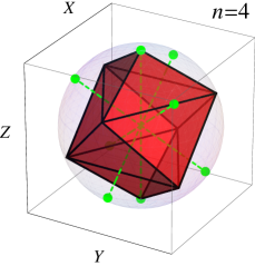
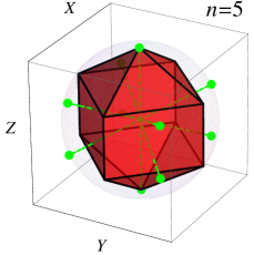
Figure 1: Bob measurement are defined by the vertex of the two solid figure for $n=4$ and $n=5$ respectively. Green points connected with dashed lines to the origin represent the pure states that saturate the LHS bound in (4).

From the inequality (4) we can derive a simpler inequality involving only one output on the Alice and Bob side. To do so it is sufficient to notice that the single qubit observables can be written as $\sigma_{b_{k}}=2\Pi^{b}_{k}-\openone$ where $\Pi^{b}_{k}$ is the projection operator on the $+1$ eigenstate of $\sigma_{b_{k}}$. Since Alice apparatus alway produces an output, we have $P(1,b|{\bf A}_{k},{\bf B}_{j})-P(-1,b|{\bf A}_{k},{\bf B}_{j})=2P(1,b|{\bf A}_{k},{\bf B}_{j})-1$. Then the correlation term $\langle{\bf A}_{k}\sigma_{b_{k}}\rangle$ can be rewritten as $4P(1,1|{\bf A}_{k},\Pi^{b}_{k})-2P_{A}(1|{\bf A}_{k})-2P_{B}(1|\Pi^{b}_{k})+1$. Since only $+1$ outcomes are involved in both Alice and Bob side, we simplify the notation as $\langle{\bf A}_{k}\sigma_{b_{k}}\rangle\equiv 4p({\bf A}_{k},\Pi^{b}_{k})-2p({\bf A}_{k})-2p(\Pi^{b}_{k})+1$. The inequality (4) can be rewritten as

$$S^{\prime}_{n}=\frac{1}{n}\sum^{n}_{k=1}\left[2p({\bf A}_{k},\Pi^{b}_{k})-p({\bf A}_{k})-p(\Pi^{b}_{k})\right]\leq C^{\prime}_{n}\,,$$ (7)

with $C^{\prime}_{n}=\frac{C_{n}-1}{2}$. The relation between the previous inequality and (4) is the same that holds between the Clauser-Horne (CH) Clauser and Horne (1974) and the CHSH Clauser et al. (1969) inequality: while in (4) correlations between two-output measurements are involved, the new inequality (7) involves only terms containing $+1$ outputs. Since the Bob measuring device is trusted his measurement can be described by a well characterized quantum observable and it is possible to consider only the events in which Bob obtains a non-null result (+1 or -1) Bennet et al. (2012). Moreover, Alice apparatus can be simplified to have only the +1 output (in fact losses are equivalent to -1 output in the inequality (7)).

Let’s now suppose that an honest Alice want to convince Bob about her ability to steer his state by using a two-qubit entangled state $\rho_{AB}$ with reduced states $\rho_{A}=\text{Tr}_{B}[\rho_{AB}]$ and $\rho_{B}=\text{Tr}_{A}[\rho_{AB}]$. Unfortunately Alice has an inefficient measuring device with $\eta$ efficiency. Alice use the projectors $\Pi^{a}_{k}$ as measurement. In this case $p({\bf A}_{k},\Pi^{b}_{k})=\eta\text{Tr}_{AB}[\Pi^{a}_{k}\otimes\Pi^{b}_{k}\rho_{AB}]$, $p({\bf A}_{k})=\eta\text{Tr}_{A}[\Pi^{a}_{k}\rho_{A}]$ and $p(\Pi^{b}_{k})=\text{Tr}_{B}[\Pi^{b}_{k}\rho_{B}]$. Alice is able to demonstrate steering only if her efficiency satisfy $\eta>\eta^{(n)}_{c}$ with the critical efficiency given by

$$\eta^{(n)}_{c} =\frac{C^{\prime}_{n}+\frac{1}{n}\sum^{n}_{k=1}\text{Tr}_{B}[\Pi^{b}_{k}\rho_{B}]}{\frac{1}{n}\sum^{n}_{k=1}\left(2\text{Tr}_{AB}[\Pi^{a}_{k}\Pi^{b}_{k}\rho_{AB}]-\text{Tr}_{A}[\Pi^{a}_{k}\rho_{A}]\right)}$$ (8)

$$=\frac{C_{n}+\frac{1}{n}\sum^{n}_{k=1}\langle\vec{b}_{k}\vec{\sigma}\rangle_{\rho_{B}}}{\frac{1}{n}\sum^{n}_{k=1}\left[\langle\vec{a}_{k}\vec{\sigma}\otimes\vec{b}_{k}\vec{\sigma}\rangle_{\rho_{AB}}+\langle\vec{b}_{k}\vec{\sigma}\rangle_{\rho_{B}}\right]}\,,$$ (9)

where $\rho_{B}$ is the reduced state on Bob side. By using maximally entangled state the best critical efficiency is given by

$$\eta^{(n)}_{c}=C_{n}\qquad\text{(for maximal entangled states)}$$ (10)

In fact for maximally entangled state we have $\rho_{B}=\frac{1}{2}\openone$ and we get $\langle\vec{b}_{k}\vec{\sigma}\rangle_{\rho_{B}}=0$ $\forall\vec{b}_{k}$. Moreover, by carefully choosing the $\vec{a}_{k}$’s it is possible to obtain $\langle\vec{a}_{k}\vec{\sigma}\otimes\vec{b}_{k}\vec{\sigma}\rangle_{\rho_{AB}}=1$ $\forall k$ and the best $\eta^{(n)}_{c}$ is equal to $C_{n}$.

Reducing $\eta_{c}$ with NMES - We now demonstrate that by using non-maximally entangled state the critical efficiency can be lowered. Let’s consider the following non-maximally entangled state:

$$|\psi\rangle=\cos\frac{\theta}{2}|01\rangle-\sin\frac{\theta}{2}|10\rangle\,,$$ (11)

and define the measuring projector as $\Pi^{a}_{k}=|a_{k}\rangle\langle a_{k}|$ and $\Pi^{b}_{k}=|b_{k}\rangle\langle b_{k}|$ with

$$|a_{k}\rangle=\sin\frac{\alpha_{k}}{2}|0\rangle-e^{i\varphi_{k}}\cos\frac{\alpha_{k}}{2}|1\rangle\,,$$ (12)

$$|b_{k}\rangle=\cos\frac{\beta_{k}}{2}|0\rangle+e^{i\phi_{k}}\sin\frac{\beta_{k}}{2}|1\rangle\,.$$

with $0\leq\phi_{k}\leq 2\pi$, $0\leq\varphi_{k}\leq 2\pi$ and $0\leq\alpha_{k}\leq\pi$. The parameter $0\leq\theta\leq\pi/2$ is an entanglement monotone Horodecki et al. (2009) and can be related to the content of entanglement of the state $|\psi\rangle$. In equation (9) only the denominator depends on the $a_{k}$’s. It is maximized (and then $\eta_{c}$ is minimized) when the $a_{k}$’s are chosen such that:

$$\tan\alpha_{k}=\sin\theta\tan\beta_{k}\,,\qquad\varphi_{k}=\phi_{k}\,.$$ (13)

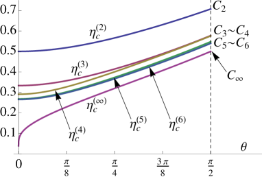
Figure 2: Critical efficiency in function of the entanglement parameter $\theta$. We report the critical efficiencies for the $n=2,\ 3,\ 4,\ 5,\ 6$ and $\infty$ setting scenario. The curves for $n=5$ is slightly higher than the $n=6$ curve.

The efficiency $\eta_{c}$ is finally minimized by the following procedure: choose the $\vec{b}_{k}$ such that the eigenvalues of the operator $\frac{1}{n}\sum_{k}\vec{b}_{k}\vec{\sigma}$ are precisely $\pm C_{n}$ and the $-C_{n}$ eigenvector is the state $|1\rangle$. By this choice we get $\frac{1}{n}\sum^{n}_{k=1}\langle\vec{b}_{k}\vec{\sigma}\rangle_{\rho_{B}}=-C_{n}\cos\theta$. The remaining term $\frac{1}{n}\sum^{n}_{k=1}\langle\vec{a}_{k}\vec{\sigma}\otimes\vec{b}_{k}\vec{\sigma}\rangle_{\rho_{AB}}$ in (9) can be calculated by means of (13). For instance, the obtained values for $n=2$ and $n=3$ are $\eta^{(2)}_{c}(\theta)=\frac{1-\cos\theta}{\sqrt{1+\sin^{2}\theta}-\cos\theta}$ and $\eta^{(3)}_{c}(\theta)=\frac{1-\cos\theta}{\sqrt{1+2\sin^{2}\theta}-\cos\theta}$. In the $n\rightarrow\infty$ limit we should replace the sum $\frac{1}{n}\sum^{n}_{k=1}$ with the integral $\frac{1}{2\pi}\int^{2\pi}_{0}\text{d}\phi\int^{1}_{0}\text{d}\cos\theta$ by considering an infinite number of $\vec{b}_{k}$ vector with positive $z$ component. In this case we obtained $\eta^{(\infty)}_{c}=1/[1+(1+\sec\theta)\text{arccosh}(\csc\theta)]$.

We report in figure 2 the values of the critical efficiencies $\eta^{(n)}_{c}$ as a function of $\theta$ for the $n=2,\ 3,\ 4,\ 5,\ 6$ and $\infty$ setting scenario. We notice that, for the maximally entangled state $\theta=\pi/2$, we get the expected result of $\eta^{(n)}_{c}=C_{n}$. We define $\bar{\eta}^{(n)}_{n}$ the limit of zero entanglement, namely $\bar{\eta}^{(n)}_{c}\equiv\lim_{\theta\rightarrow 0}\eta^{(n)}_{c}(\theta)$. It is worth noting that $\bar{\eta}^{(n)}_{c}$ is always lower than $C_{n}$ and an arbitrary low value can be obtained by increasing the number $n$ of observables. In fact we have $\bar{\eta}^{(2)}_{c}=\frac{1}{2}$, $\bar{\eta}^{(3)}_{c}=\frac{1}{3}$, $\bar{\eta}^{(4)}_{c}\simeq 0.291$, $\bar{\eta}^{(5)}_{c}\simeq 0.268$, , $\bar{\eta}^{(6)}_{c}\simeq 0.266$, …, $\bar{\eta}^{(\infty)}_{c}=0$.

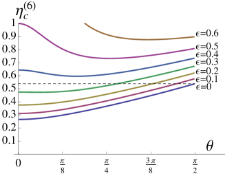
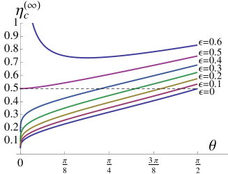
Figure 3: Values of $\eta^{(noise)}_{c}$ in function of $\theta$ for different noise parameter $\epsilon$ in the case of $n=6$ (top graph) and $n=\infty$ (bottom graph) measurement settings. With dashed line we show the value of $C_{6}$ and $C_{\infty}$ respectively to compare with the efficiency required with non-noisy maximally entangled state.

We can also calculate how the critical efficiency changes if the NMES is noisy. Here we consider a colored noise model, in which the shared state is given by

$$\rho =(1-\epsilon)|\psi\rangle\langle\psi|+\epsilon\rho_{noise}$$ (14)

$$\rho_{noise} =\cos^{2}\frac{\theta}{2}|01\rangle\langle 01|+\sin^{2}\frac{\theta}{2}|10\rangle\langle 10|$$

There are two main reasons to consider colored and not white (corresponding to $\rho_{noise}=\frac{1}{4}\openone$) noise: first of all, when the entangled state (11) is experimentally generated, for example by spontaneous parametric down conversion, the main source of imperfection comes from the difficulty of producing $|01\rangle$ and $|10\rangle$ perfectly indistinguishable: this introduces a decoherence precisely corresponding to our colored noise model. Moreover, the white noise will require higher efficiency since the advantage of using NMES comes from the ”polarization” of single qubit reduced states $\rho_{A}$ and $\rho_{B}$, while white noise is completely ”depolarized”. On the other side, in the colored noise model, the reduced states $\rho_{A}$ and $\rho_{B}$ are not dependent on $\epsilon$ and the state $\rho$ is entangled for any $\epsilon>0$. In fact, when white noise is introduced the critical efficiency is changed into $\eta^{(white)}_{c}(\theta)=\left[1+\frac{\epsilon}{2(1-\epsilon)\sin^{2}\frac{\theta}{2}}\right]\eta_{c}(\theta)$ and the limit for $\theta\rightarrow 0$ is always diverging for any low value of the noise parameter $\epsilon$. On the other hand, the critical efficiency $\eta^{(noise)}_{c}$ obtained by using the noise model (14) can be written as $\frac{1}{\eta^{(noise)}_{c}}=\frac{1-\epsilon}{\eta^{(n)}_{c}}+\epsilon\frac{\frac{1}{n}\sum^{n}_{k=1}\langle\vec{a}_{k}\vec{\sigma}\otimes\vec{b}_{k}\vec{\sigma}\rangle_{\rho_{noise}}-C_{n}\cos\theta}{C_{n}(1-\cos\theta)}$. We show in figure 3 the values of $\eta^{(noise)}_{c}$ in function of $\theta$ for different noise parameter $\epsilon$ in the case of $n=6$ (top graph) and $n=\infty$ (bottom graph) measurement settings. It is worth noting that, even with high values of the noise, by using NMES it is possible to obtain a critical efficiency that is lower than the one obtained by maximal entangled states. With 6 measurements and up to $35\%$ noise, NMES outperform maximally entangled states in the required detection efficiency for a loophole free experiment.

Conclusions - In this work we showed that the inequality introduced in Saunders et al. (2010) can be violated with arbitray low efficiency by using non-maximally entangled state. This feature resembles the property of NMES to better violate Bell inequalities in presence of detection inefficiencies. The violation of the steering inequality is proven to be highly resistant against decoherence, the most common noise present in actual experiments. For example, with $10\%$ noise, the inequality can be violated by using 6 measurements and detection efficiency larger than $31.14\%$. Our result can have important application in quantum cryptography due to the recent connection between steering and cryptography Branciard et al. (2012). This could be particular relevant for long distance quantum communication with high losses Villoresi et al. (2008), in which the trusted device is located at distance with respect to the entanglement source while the untrusted device is placed close to the source to achieve the required efficiency needed to violate a steering inequality.