Order-$v^{4}$ Relativistic Corrections to $\Upsilon$ Inclusive Decay into a Charm pair

Abstract

In this work, we determine the short-distance coefficients for $\Upsilon$ inclusive decay into a charm pair through relative order $v^{4}$ within the framework of NRQCD factorization formula. The short-distance coefficient of the order-$v^{4}$ color-singlet NRQCD matrix element is obtained through matching the decay rate of $b\bar{b}(^{3}S^{[1]}_{1})\to c\bar{c}gg$ in full QCD to that in NRQCD. The double and single IR divergences appearing in the decay rate are exactly canceled through the next-to-next-to-leading-order renormalization of the operator ${\mathcal{O}}(^{3}S^{[8]}_{1})$ and the next-to-leading-order renormalization of the operators ${\mathcal{O}}(^{3}P^{[8]}_{J})$. To investigate the convergence of the relativistic expansion arising from the color-singlet contributions, we study the ratios of the order-$v^{2}$ and -$v^{4}$ color-singlet short-distance coefficients to the leading-order one. Our results indicate that though the order-$v^{4}$ color-singlet short-distance coefficient is quite large, the relativistic expansion for the color-singlet contributions in the process $\Upsilon\to c\bar{c}+X$ is well convergent due to a small value of $v$. In addition, we extrapolate the value of the mass ratio of the charm quark to the bottom quark, and find the relativistic corrections rise quickly with increase of the mass ratio.

I Introduction

NRQCD factorization formula Bodwin:1994jh provides a systematical approach to express the quarkonium inclusive decay rate (cross section) as the sum of product of short-distance coefficients and the NRQCD matrix elements. The short-distance coefficients can be expanded as perturbation series in coupling constant $\alpha_{s}$ at the scale of the heavy quark mass $m$. The long-distance matrix elements can be expressed in a definite way with the typical relative velocity $v$ of the heavy quark in the quarkonium.

The relativistic corrections to the quarkonium decay and production have been widely studied. In some processes, the next-to-leading-order (NLO) relativistic corrections are sizable, some of which even surpass the leading-order (LO) contributions. For the quarkonium production, typical examples are the double charmonia $J/\psi+\eta_{c}$ production at the B factories Braaten:2002fi ; He:2007te and the double $\eta_{c}$ production through $\eta_{b}$ decay Sang:2011fw . For the quarkonium annihilate decay, it happens in the $J/\psi$ inclusive decay and $J/\psi(\Upsilon)$ inclusive decay into a lepton pair or charm pair Keung:1982jb ; Chen:2011ph ; Chen:2012zzg . It may arouse worries about the relativistic expansion in the NRQCD approach. In Refs. Bodwin:2006ke ; Bodwin:2007ga , the authors resumed a collect of relativistic corrections to the process $e^{+}e^{-}\to J/\psi+\eta_{c}$ and found the relativistic expansion is of well convergence. Similarly, the authors of Ref. Sang:2011fw studied the process $\eta_{b}\to\eta_{c}(mS)\eta_{c}(nS)$ and found the relativistic expansion is convergent very well, though the order-$v^{2}$ corrections are both negative and large. In Ref. Bodwin:2002hg , the authors considered the order-$v^{4}$ corrections to $J/\psi$ inclusive decay and found the contribution from the color-singlet matrix element in this order is not as large as the LO and NLO contributions. The order-$v^{6}$ corrections to this process were even calculated in Ref. Chung:TBD , where the convergence is furthermore confirmed.

It has been shown that the order-$v^{2}$ corrections to the process $\Upsilon\to c\bar{c}+X$ are extremely huge Chen:2011ph . The ratio of the short-distance coefficient of the order-$v^{2}$ matrix element to that of the LO one approaches to $-12$. It seriously spoils the relativistic expansion. So it urges us to calculate the order-$v^{4}$ corrections and investigate the convergence of the relativistic expansion for this process. Moreover, since the momenta of some gluons can be simultaneously soft, there exist complicated IR divergences in the calculations. It is technically challenging to cancel the IR divergences and obtain the IR-independent short-distance coefficients through the color-octet mechanism , and it also provides an example to examine the NRQCD factorization formula.

The remainder of this paper is organized as follows. In Sec. II, we describe the NRQCD factorization formula for the $\Upsilon$ inclusive decay into a charm pair. In Sec. III, we list our definitions and present the techniques used to compute the decay rates. We elaborate the calculations on determining the short-distance coefficients at relative order $v^{4}$ in Sec. IV. The QCD corrections to the color-octet operators are also calculated in this section. Sec. V is devoted to discussions and summaries.

II NRQCD factorization formula for $\Upsilon\to c\bar{c}+X$

According to the NRQCD factorization formula, through relative order $v^{4}$, the differential decay rate for $\Upsilon$ inclusive decay into a charm pair can be expressed as Bodwin:1994jh :

$$d\Gamma[\Upsilon\to c\bar{c}+X] = \frac{dF_{1}({}^{3}S^{[1]}_{1})}{m^{2}}\langle\mathcal{O}({}^{3}S^{[1]}_{1})\rangle_{\Upsilon}+\frac{dF_{2}({}^{3}S^{[1]}_{1})}{m^{4}}\langle\mathcal{P}({}^{3}S^{[1]}_{1})\rangle_{\Upsilon}+\frac{dF({}^{1}S^{[8]}_{0})}{m^{2}}\langle\mathcal{O}({}^{1}S^{[8]}_{0})\rangle_{\Upsilon}$$ (1)

$$+\frac{dF_{3}({}^{3}S^{[1]}_{1})}{m^{6}}\langle\mathcal{Q}_{1}({}^{3}S^{[1]}_{1})\rangle_{\Upsilon}+\frac{dF_{4}({}^{3}S^{[1]}_{1})}{m^{6}}\langle\mathcal{Q}_{2}({}^{3}S^{[1]}_{1})\rangle_{\Upsilon}$$

$$+\frac{dF({}^{3}S^{[8]}_{1})}{m^{2}}\langle\mathcal{O}({}^{3}S^{[8]}_{1})\rangle_{\Upsilon}+\sum_{J=0,1,2}\frac{dF({}^{3}P^{[8]}_{J})}{m^{4}}\langle\mathcal{O}({}^{3}P^{[8]}_{J})\rangle_{\Upsilon},$$

where $m$ indicates the mass of the bottom quark $b$, $\mathcal{O}({}^{2S+1}L^{[c]}_{J})$ indicates the NRQCD operator with the spectroscopic state ${}^{2S+1}L^{[c]}_{J}$ with the spin $S$, orbital angular momentum $L$, total angular momentum $J$, and color quantum number $c$, and $\langle\mathcal{O}({}^{2S+1}L^{[c]}_{J})\rangle_{H}\equiv\langle H|\mathcal{O}({}^{2S+1}L^{[c]}_{J})|H\rangle$ indicates the NRQCD matrix element averaged over the spin states of $H$. The color quantum number $c=1$ and $8$ in the NRQCD operators denote the color-singlet and the color-octet respectively. The NRQCD operators in the factorization formula (1) are defined by 

$$\mathcal{O}({}^{3}S^{[1]}_{1}) = \psi^{\dagger}\bm{\sigma}\chi\cdot\chi^{\dagger}\bm{\sigma}\psi,$$ (2a)

$$\mathcal{P}({}^{3}S^{[1]}_{1}) = \frac{1}{2}\bigg{[}\psi^{\dagger}\bm{\sigma}\chi\cdot\chi^{\dagger}\big{(}-\tfrac{i}{2}\overleftrightarrow{\bm{D}}\big{)}^{2}\bm{\sigma}\psi+\psi^{\dagger}\big{(}-\tfrac{i}{2}\overleftrightarrow{\bm{D}}\big{)}^{2}\bm{\sigma}\chi\cdot\chi^{\dagger}\bm{\sigma}\psi\bigg{]},$$ (2b)

$$\mathcal{O}({}^{3}S^{[8]}_{1}) = \psi^{\dagger}\bm{\sigma}T^{a}\chi\cdot\chi^{\dagger}\bm{\sigma}T^{a}\psi,$$ (2c)

$$\mathcal{O}({}^{1}S^{[8]}_{0}) = \psi^{\dagger}T^{a}\chi\cdot\chi^{\dagger}T^{a}\psi,$$ (2d)

$$\mathcal{O}({}^{3}P^{[8]}_{0}) = \frac{1}{d-1}\psi^{\dagger}\big{(}-\tfrac{i}{2}\overleftrightarrow{\bm{D}}\cdot\bm{\sigma}\big{)}T^{a}\chi\cdot\chi^{\dagger}\big{(}-\tfrac{i}{2}\overleftrightarrow{\bm{D}}\cdot\bm{\sigma}\big{)}T^{a}\psi,$$ (2e)

$$\mathcal{O}({}^{3}P^{[8]}_{1}) = \psi^{\dagger}\big{(}-\tfrac{i}{2}\overleftrightarrow{{D}}{}^{[i,}\sigma^{j]}\big{)}T^{a}\chi\cdot\chi^{\dagger}\big{(}-\tfrac{i}{2}\overleftrightarrow{{D}}{}^{[i,}\sigma^{j]}\big{)}T^{a}\psi,$$ (2f)

$$\mathcal{O}({}^{3}P^{[8]}_{2}) = \psi^{\dagger}\big{(}-\tfrac{i}{2}\overleftrightarrow{{D}}{}^{(i,}\sigma^{j)}\big{)}T^{a}\chi\cdot\chi^{\dagger}\big{(}-\tfrac{i}{2}\overleftrightarrow{{D}}{}^{(i,}\sigma^{j)}\big{)}T^{a}\psi,$$ (2g)

$$\mathcal{Q}_{1}({}^{3}S^{[1]}_{1}) = \psi^{\dagger}\big{(}-\tfrac{i}{2}\overleftrightarrow{\bm{D}}\big{)}^{2}\bm{\sigma}\chi\cdot\chi^{\dagger}\big{(}-\tfrac{i}{2}\overleftrightarrow{\bm{D}}\big{)}^{2}\bm{\sigma}\psi,$$ (2h)

$$\mathcal{Q}_{2}({}^{3}S^{[1]}_{1}) = \frac{1}{2}\bigg{[}\psi^{\dagger}\bm{\sigma}\chi\cdot\chi^{\dagger}\big{(}-\tfrac{i}{2}\overleftrightarrow{\bm{D}}\big{)}^{4}\bm{\sigma}\psi+\psi^{\dagger}\big{(}-\tfrac{i}{2}\overleftrightarrow{\bm{D}}\big{)}^{4}\bm{\sigma}\chi\cdot\chi^{\dagger}\bm{\sigma}\psi\bigg{]},$$ (2i)

where $\psi$ and $\chi$ are Pauli spinor fields that annihilates the bottom quark and creates the bottom antiquark, respectively, $\sigma^{i}$ denotes the Pauli matrix, $\overleftrightarrow{\bm{D}}$ indicates the gauge-covariant derivative, and $d=4-2\epsilon$ represents the space-time dimensions. In (2), $A^{[i,}B^{j]}$ and $A^{(i,}B^{j)}$ indicate the antisymmetric tensor and the symmetric traceless tensor respectively, which are defined via Bodwin:2012xc

$$A^{[i,}B^{j]} \equiv \frac{1}{2}(A^{i}B^{j}-A^{j}B^{i}),$$ (3a)

$$A^{(i,}B^{j)} \equiv \frac{1}{2}(A^{i}B^{j}+A^{j}B^{i})-\frac{1}{d-1}\delta^{ij}A^{k}B^{k}.$$ (3b)

In (1), we omit the term associated with the matrix element of the operator

$$\frac{1}{2}\bigg{[}\psi^{\dagger}\bm{\sigma}\chi\cdot\chi^{\dagger}\big{(}\overleftrightarrow{\bm{D}}\cdot g{\bm{E}}+g{\bm{E}}\cdot\overleftrightarrow{\bm{D}}\big{)}\bm{\sigma}\psi-\psi^{\dagger}\big{(}\overleftrightarrow{\bm{D}}\cdot g{\bm{E}}+g{\bm{E}}\cdot\overleftrightarrow{\bm{D}}\big{)}\bm{\sigma}\chi\cdot\chi^{\dagger}\bm{\sigma}\psi\bigg{]},$$ (4)

which is shown to be dependent and be a linear combination of the matrix elements of the operators (2h) and (2i) accurate up to relative order $v^{4}$ Bodwin:2002hg .

In order to get the decay rate, both the NRQCD matrix elements and the short-distance coefficients in (1) should be determined. The NRQCD matrix elements have been studied through many nonperturbative approaches, such as lattice QCD Bodwin:1993wf , nonrelativistic quark model Eichten:1995 , and fitting the experimental data Bodwin:2007fz ; Guo:2011tz .

On the other hand, based on the factorization, the short-distance coefficients can be perturbatively determined through matching the decay rates of the relevant processes at parton level in full QCD to these in NRQCD. At the leading order in $\alpha_{s}$, the coefficients $dF(^{1}S^{[8]}_{0})$, $dF(^{3}S^{[8]}_{1})$, and $dF(^{3}P^{[8]}_{J})$ can be determined through the processes $b\bar{b}(^{1}S^{[8]}_{0})\to c\bar{c}g$, $b\bar{b}(^{3}S^{[8]}_{1})\to c\bar{c}$, and $b\bar{b}(^{3}P^{[8]}_{J})\to c\bar{c}g$ respectively. The color-singlet short-distance coefficients can be determined through the process $b\bar{b}(^{3}S^{[1]}_{1})\to c\bar{c}gg$. Among these short-distance coefficients, $F(^{3}S^{[8]}_{1})$ has been calculated up to the next-to-leading order in $\alpha_{s}$ in Ref. Zhang:2008pr . $F_{1}(^{3}S^{[1]}_{1})$ and $F_{2}(^{3}S^{[1]}_{1})$ are obtained in Refs. Fritzsch:1978ey ; Parkhomenko:1994xi ; Kang:2007uv and Refs. Chen:2011ph ; Chen:2012zzg , respectively.

As mentioned in Ref. Bodwin:2002hg , since there exists the relation $\langle\mathcal{Q}_{2}({}^{3}S^{[1]}_{1})\rangle_{\Upsilon}=\langle\mathcal{Q}_{1}({}^{3}S^{[1]}_{1})\rangle_{\Upsilon}(1+\mathcal{O}(v^{2}))$, to order $v^{4}$, we can only determine the sum of the short-distance coefficients: 

$$dF(^{3}S^{[1]}_{1})\equiv dF_{3}(^{3}S^{[1]}_{1})+dF_{4}(^{3}S^{[1]}_{1}).$$ (5)

As we will see, in order to get the IR-independent coefficient $dF(^{3}S^{[1]}_{1})$, we are required to calculate $dF(^{3}S^{[8]}_{1})$ and $dF(^{3}P^{[8]}_{J})$, and make use of the color-octet mechanism to cancel the IR divergences appearing in the decay rate of the process $b\bar{b}(^{3}S^{[1]}_{1})\to c\bar{c}gg$.

III kinematic definitions and phase-space decompositions

III.1 Kinematic definitions

We assign $m_{c}$ to the mass of charm quark, and assign $p_{1}$ and $p_{2}$ to the momenta of the incoming bottom quark $b$ and antiquark $\bar{b}$. The momenta satisfy the on-shell relations: $p_{1}^{2}=p_{2}^{2}=m^{2}$. $p_{1}$ and $p_{2}$ can be expressed as linear combinations of their total momentum $P$ and half their relative momentum $p$:

$$p_{1}=P/2+p,\,\,\,\,\,\,\,\,\,\,\,\,p_{2}=P/2-p.$$ (6)

We assign $l_{1},l_{2}$ to the momenta of the final charm pair. Therefore the momentum of the virtual gluon yields to $Q=l_{1}+l_{2}$. In addition, we take $k_{1}$ to the momentum of the gluon in the process $b\bar{b}\to c\bar{c}g$, and take $k_{1},k_{2}$ to the momenta of the two gluons in the process $b\bar{b}\to c\bar{c}gg$.

To facilitate the evaluation, we introduce a set of dimensionless variables

$$x_{1}=\frac{2k_{1}\cdot P}{P^{2}},\,\,x_{2}=\frac{2k_{2}\cdot P}{P^{2}},\,\,z=\frac{Q^{2}}{P^{2}},\,\,r=\frac{4m_{c}^{2}}{M^{2}},$$ (7)

where $M$ denotes the mass of the bottomonium. At the leading order in $v$, there is $M=2m$. All the Lorentz invariant kinematic quantities can be expressed in terms of these new variables.

III.2 Phase-space decompositions

In this subsection, we present the techniques for phase-space calculations of the relevant processes. We decompose each phase-space integral into two parts, which is proved to significantly simplify the calculations in the following section.

III.2.1 $b\bar{b}({}^{3}S^{[1]}_{1})\to c\bar{c}gg$

The process $b\bar{b}({}^{3}S^{[1]}_{1})\to c\bar{c}gg$ involves four-body phase-space integral, which can be expressed as

$$\int\!\!d\phi_{4} = \!\!\!\int\!\!\!{d^{d-1}k_{1}\over(2\pi)^{d-1}2k^{0}_{1}}{d^{d-1}k_{2}\over(2\pi)^{d-1}2k^{0}_{2}}{d^{d-1}l_{1}\over(2\pi)^{d-1}2l^{0}_{1}}{d^{d-1}l_{2}\over(2\pi)^{d-1}2l^{0}_{2}}(2\pi)^{d}\delta^{d}(P-k_{1}-k_{2}-l_{1}-l_{2}).$$ (8)

As the treatment in Ref. Chen:2011ph , we decompose the space-space integral into

$$\int\!\!d\phi_{4}=\!\!\!\int\!\!{dz\over 2\pi}\int\!\!d\phi_{3-1}\!\!\int\!\!d\phi_{2-1},$$ (9)

where $\int\!\!d\phi_{3-1}$ and $\int\!\!d\phi_{2-1}$ are defined via

$$\int\!\!d\phi_{3-1} = \!\!\!\int\!\!{d^{d-1}Q\over(2\pi)^{d-1}2Q^{0}}{d^{d-1}k_{1}\over(2\pi)^{d-1}2k^{0}_{1}}{d^{d-1}k_{2}\over(2\pi)^{d-1}2k^{0}_{2}}(2\pi)^{d}\delta^{d}(P-k_{1}-k_{2}-Q),$$ (10a)

$$\int\!\!d\phi_{2-1} = \!\!P^{2}\!\!\int\!\!{d^{d-1}l_{1}\over(2\pi)^{d-1}2l^{0}_{1}}{d^{d-1}l_{2}\over(2\pi)^{d-1}2l^{0}_{2}}(2\pi)^{d}\delta^{d}(Q-l_{1}-l_{2}).$$ (10b)

On the other hand, we can also separate the squared amplitude of the process into two parts: the charm part and the bottom part, i.e.,

$$\sum_{pol,col}|{\cal M}(^{3}S^{[1]}_{1})|^{2}={L}^{(ab)\mu\nu}{H}^{(ab)}_{\mu\nu}(^{3}S^{[1]}_{1}),$$ (11)

where polarizations and colors of the initial and final states are summed, $a,b$ denote the color indices, and the charm part ${L}^{(ab)\mu\nu}$ is given by

$${L}^{(ab)\mu\nu}=\frac{\delta^{ab}}{2}\frac{g_{s}^{2}}{Q^{4}}{\rm Tr}[(\not\!l_{1}+m_{c})\gamma^{\mu}(\not\!l_{2}-m_{c})\gamma^{\nu}],$$ (12)

and the bottom part ${H}^{(ab)}_{\mu\nu}(^{3}S^{[1]}_{1})$ accounts for the remainder. According to the current conservation, we have

$$\int\!\!d\phi_{2-1}{L}^{(ab)\mu\nu}=\frac{\delta^{ab}}{2}\bigg{(}\!\!-g^{\mu\nu}+\frac{Q^{\mu}Q^{\nu}}{Q^{2}}\bigg{)}\times L,$$ (13)

where the Lorentz invariance $L$ is explicitly calculated

$$L={\alpha_{s}\over 3z}(2+\frac{r}{z})\sqrt{1-{r\over z}}.$$ (14)

As we will see, since $L$ is a common factor in the whole calculations, we get (14) in 4-dimensions. As a consequence, the decay rate yields

$$\Gamma(^{3}S^{[1]}_{1})=\frac{1}{2}\int\!\!\frac{dz}{2\pi}L\int\!\!d\phi_{3-1}\frac{\delta^{ab}}{2}{\widetilde{H}}^{(ab)}_{\mu\nu}(^{3}S^{[1]}_{1})\bigg{(}-g^{\mu\nu}+\frac{Q^{\mu}Q^{\nu}}{Q^{2}}\bigg{)},$$ (15)

where a symmetry factor $\tfrac{1}{2}$ is included to account for the indistinguishability of the two gluons. The second term in the parenthesis of (15) does not contribute, due to the current conservation.

It is accustomed to reduce $\int\!\!d\phi_{3-1}$ into the integration over two dimensionless variables:

$$\int\!\!d\phi_{3-1}=\frac{P^{2}}{128\pi^{3}}\frac{f_{\epsilon}^{2}e^{2\epsilon\gamma_{E}}}{\Gamma(2-2\epsilon)}\int\!\!\!dx_{1}dx_{2}\bigg{\{}(x_{1}+x_{2}-1+z)[(1-x_{1})(1-x_{2})-z]\bigg{\}}^{-\epsilon}\!\!\!\!\!\!.\phantom{x}$$ (16)

where $f_{\epsilon}\equiv(\tfrac{4\pi\mu^{2}}{M^{2}}e^{-\gamma_{E}})^{\epsilon}$. Here $\mu$ in $f_{\epsilon}$ represents the dimensional-regularization scale, and $\gamma_{E}$ denotes the Euler constant. The boundaries of $z,x_{1}$, and $x_{2}$ are readily inferred

$$1-x_{1}-z\leq x_{2}\leq{1-x_{1}-z\over 1-x_{1}},\ \ \ 0\leq x_{1}\leq 1-z,\ \ \ r\leq z\leq 1.$$ (17)

It is convenient to make a further change of variables:

$$x_{1}=(1-z)x,\,\,\,\,\,\,\,\,\,x_{2}=\frac{(1-z)(1-x)[1-(1-z)xy]}{1-(1-z)x}.$$ (18)

This change of variables is particularly useful in extracting the relativistic corrections. Through this transformation, the boundaries of the new variables are simplified to

$$0\leq x\leq 1,\,\,\,\,\,\,\,\,\,\,\,\,\,0\leq y\leq 1.$$ (19)

Finally, the decay rate reduces to

$$\Gamma(^{3}S^{[1]}_{1})=\frac{f_{\epsilon}^{2}e^{2\epsilon\gamma_{E}}}{\Gamma(2-2\epsilon)}\int\!\!dzdxdy\bigg{[}\frac{1-(1-z)x}{y(1-y)x^{2}(1-x)^{2}}\bigg{]}^{\epsilon}(1-z)^{-4\epsilon}L\times H(^{3}S^{[1]}_{1}),$$ (20)

where

$$H(^{3}S^{[1]}_{1})\equiv\frac{1}{2}\frac{P^{2}(1-z)^{3}}{(4\pi)^{4}}\frac{x(1-x)}{1-(1-z)x}\frac{\delta^{ab}}{2}(-g^{\mu\nu}){\widetilde{H}}^{(ab)}_{\mu\nu}(^{3}S^{[1]}_{1}).$$ (21)

III.2.2 $b\bar{b}(^{3}P^{[8]}_{J})\to c\bar{c}g$

Analogously, we separate the phase-space integral of this process into

$$\int\!\!d\phi_{3-2}=\int\!\!{dz\over 2\pi}\int\!\!d\phi_{2-1}\!\!\!\int\!\!d\phi_{2-2},$$ (22)

where $\int\!\!d\phi_{2-1}$ is given in (10b) and $\int\!\!d\phi_{2-2}$ indicates

$$\int\!\!d\phi_{2-2} = \int\!\!{d^{d-1}Q\over(2\pi)^{d-1}2Q^{0}}{d^{d-1}k_{1}\over(2\pi)^{d-1}2k^{0}_{1}}(2\pi)^{d}\delta^{d}(P-k_{1}-Q).$$ (23)

$\int\!\!d\phi_{2-2}$ can be straightforward integrated out as

$$\int\!\!d\phi_{2-2}=\frac{(1-z)^{1-2\epsilon}}{8\pi}\frac{\Gamma(1-\epsilon)}{\Gamma(2-2\epsilon)\Gamma(1+\epsilon)}f_{\epsilon},$$ (24)

Similarly, we separate the squared amplitude into the charm part and the bottom part ${H}^{ab}_{\mu\nu}(^{3}P^{[8]}_{J})$, and obtain the decay rate

$$\Gamma=\frac{\Gamma(1-\epsilon)f_{\epsilon}e^{\epsilon\gamma_{E}}}{\Gamma(2-2\epsilon)}\int\!\!dz(1-z)^{-2\epsilon}L\times H(^{3}P^{[8]}_{J}),$$ (25)

where

$$H(^{3}P^{[8]}_{J}) \equiv \frac{\delta^{ab}}{2}\frac{(1-z)(-g^{\mu\nu}){H}^{ab}_{\mu\nu}(^{3}P^{[8]}_{J})}{16\pi^{2}}.$$ (26)

III.2.3 $b\bar{b}(^{3}S^{[8]}_{1})\to c\bar{c}$

The phase-space integral of this process is quite simple. Therefore we directly present the decay rate

$$\Gamma(^{3}S^{[8]}_{1})=\int\!\!dz\delta(1-z)H(^{3}S^{[8]}_{1})\times L,$$ (27)

where $H(^{3}S^{[8]}_{1})$ is defined via

$$H(^{3}S^{[8]}_{1})\equiv\frac{\delta^{ab}}{2}\frac{(-g^{\mu\nu}){H}^{ab}_{\mu\nu}(^{3}S^{[8]}_{1})}{P^{2}}.$$ (28)

IV Determining the short-distance coefficients

In this section, we determine the differential short-distance coefficients of $\Upsilon$ include decay into a charm pair at relative order $v^{4}$. $dF(^{3}S^{[8]}_{1})$, $dF(^{3}P^{[8]}_{J})$, and $dF(^{3}S^{[1]}_{1})$ can be determined through calculating the decay rates of the perturbative processes $b{\bar{b}}(^{3}S^{[8]}_{1})\to c\bar{c}$, $b{\bar{b}}(^{3}P^{[8]}_{J})\to c\bar{c}g$, and $b{\bar{b}}(^{3}S^{[1]}_{1})\to c\bar{c}gg$, respectively.

IV.1 $S$-wave color-octet

We first determine the differential short-distance coefficient $dF({}^{3}S^{[8]}_{1})$ through matching the decay rate of $b\bar{b}({{}^{3}S^{[8]}_{1}})\to c\bar{c}$ in full QCD to that in NRQCD. We also carry out the computations for the renormalization of the operator ${\mathcal{O}}(^{3}S^{[8]}_{1})$, which will produce mixing with the operator ${\mathcal{O}}(^{3}P^{[8]}_{J})$ at the next-to-leading order in $\alpha_{s}$ and with the operator ${\mathcal{O}}(^{3}S^{[1]}_{1})$ at the next-to-next-to-leading order in $\alpha_{s}$. Moreover we consider the renormalization of the operators ${\mathcal{O}}(^{3}P^{[8]}_{J})$, which will induce mixing with the operator ${\mathcal{O}}(^{3}S^{[1]}_{1})$. The renormalized operators will be utilized to cancel the IR divergences through the color-octet mechanism when we determine the differential short-distance coefficients $dF(^{3}P^{[8]}_{J})$ and $dF(^{3}S^{[1]}_{1})$.

IV.1.1 $dF({{}^{3}S^{[8]}_{1}})$

The corresponding factorization formula for $b\bar{b}({{}^{3}S^{[8]}_{1}})\to c\bar{c}$ is expressed as

$$\frac{d\Gamma(^{3}S^{[8]}_{1})}{dz} = \frac{dF({}^{3}S^{[8]}_{1})}{m^{2}dz}\langle\mathcal{O}({}^{3}S^{[8]}_{1})\rangle_{b\bar{b}(^{3}S^{[8]}_{1})}\,.$$ (29)

Through calculations, we obtain the expression of $H(^{3}S^{[8]}_{1})$ defined in (28) as

$$H(^{3}S^{[8]}_{1})=\frac{\pi\alpha_{s}}{2m^{2}}.$$ (30)

Inserting (30) into (27), we immediately deduce the differential decay rate in full QCD. By making use of $\langle\mathcal{O}({}^{3}S^{[8]}_{1})\rangle_{b\bar{b}(^{3}S^{[8]}_{1})}=1$, where the quark pair state is non-relativistically normalized, we readily get

$$\frac{dF({}^{3}S^{[8]}_{1})}{dz} = \delta(1-z)\frac{\pi\alpha_{s}}{2}\times L.$$ (31)

IV.1.2 ${}^{3}S^{[8]}_{1}\to{}^{3}P^{[8]}_{J}$

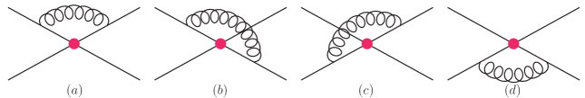
Figure 1: The Feynman graphs for the NLO QCD corrections to the operator ${\mathcal{O}}(^{3}S^{[8]}_{1})$. We suppress the graphs which do not give rise to operator mixing.

In this subsection, we consider the NLO QCD corrections to the operator ${\mathcal{O}}(^{3}S^{[8]}_{1})$. There are four diagrams illustrated in Fig. 1 . The vertex in the middle signifies the operator ${\mathcal{O}}(^{3}S^{[8]}_{1})$. Since the diagrams involve UV divergences, the operator needs to be renormalized. In this work, we uniformly use $\overline{\rm MS}$ scheme to carry out renormalization. We express the renormalized operator as

$${\mathcal{O}}(^{3}S^{[8]}_{1})_{\overline{\rm MS}}={\mathcal{O}}(^{3}S^{[8]}_{1})+\delta_{1}{}{\mathcal{O}}+\delta_{2}{}{\mathcal{O}}+{\cal O}(\alpha_{s}^{3}),$$ (32)

where we truncate the expansion up to order $\alpha_{s}^{2}$, which is enough to current work. $\delta_{1}{}{\mathcal{O}}$ and $\delta_{2}{}{\mathcal{O}}$ are the corresponding NLO and the next-to-next-to-leading-order (NNLO) counterterms respectively. For convenience, we can expand an operator ${\mathcal{O}}$ in terms of $\alpha_{s}$:

$${\mathcal{O}}={\mathcal{O}}^{(0)}+{\mathcal{O}}^{(1)}+{\mathcal{O}}^{(2)}+\cdots.$$ (33)

where the superscript ‘(n)’ represents order-$\alpha_{s}^{n}$ contribution.

In the following calculations, we will also utilize the color decompositions Petrelli:1997ge

$$T^{a}T^{b}\otimes T^{a}T^{b} = \frac{N_{c}^{2}-1}{4N_{c}^{2}}1\otimes 1-\frac{1}{N_{c}}T^{a}\otimes T^{a},$$

$$T^{a}T^{b}\otimes T^{b}T^{a} = \frac{N_{c}^{2}-1}{4N_{c}^{2}}1\otimes 1+\frac{N_{c}^{2}-2}{2N_{c}}T^{a}\otimes T^{a}.$$ (34a)

With the NRQCD Feynman rules Bodwin:1998mn , the color-octet contribution from Fig. 1(a) reads

$$I_{a} = \frac{(ig_{s})^{2}}{4m^{2}}\frac{-1}{N_{c}}T^{a}\otimes T^{a}\int\frac{d^{d}k}{(2\pi)^{d}}\frac{i}{p^{0}-k^{0}-\frac{(\vec{{\bm{p}}}-\vec{{\bm{k}}})^{2}}{2m}+i\epsilon}\frac{i}{p^{\prime 0}-k^{0}-\frac{(\vec{{\bm{p}}^{\prime}}-\vec{{\bm{k}}})^{2}}{2m}+i\epsilon}$$ (35)

$$\times\frac{4i({\bm{p}}\cdot{\bm{p}}^{\prime}-{\bm{p}}\cdot{\bm{k}}{\bm{p}}^{\prime}\cdot{\bm{k}}/{\bm{k}}^{2})}{k^{2}+i\epsilon}$$

$$= -\frac{g_{s}^{2}}{2m^{2}}\frac{T^{a}\otimes T^{a}}{N_{c}}{\bm{p}}\cdot{\bm{p}}^{\prime}\frac{d-2}{d-1}\int\frac{d^{d-1}k}{(2\pi)^{d-1}}\frac{1}{|{\bm{k}}|^{3}}$$

$$= -\frac{\alpha_{s}}{3\pi m^{2}}\frac{T^{a}\otimes T^{a}}{N_{c}}\bigg{(}\frac{\tilde{f}_{\epsilon}}{\epsilon_{\rm UV}}-\frac{\tilde{f}_{\epsilon}}{\epsilon_{\rm IR}}\bigg{)}{\bm{p}}\cdot{\bm{p}}^{\prime},$$

where $\tilde{f}_{\epsilon}\equiv(4\pi e^{-\gamma_{E}})^{\epsilon}$. Since the coefficient is proportional to $\frac{1}{\epsilon_{\rm UV}}-\frac{1}{\epsilon_{\rm IR}}$, the factor $d$ coming from the loop integral in (35) is replaced with $4$ in the ${\overline{\rm MS}}$ scheme. Moreover, we add the factor $\tilde{f}_{\epsilon}$ which is always associated with the $\overline{\rm MS}$ scheme.

It is not hard to find that Fig. 1(b-d) give the same contributions as Fig. 1(a) up to a color factor. Summing all the contributions and employing (32), we get

$${\mathcal{O}}(^{3}S^{[8]}_{1})_{\overline{\rm MS}} = {\mathcal{O}}(^{3}S^{[8]}_{1})^{(0)}-\frac{5\alpha_{s}}{9\pi m^{2}}\frac{\tilde{f}_{\epsilon}}{\epsilon_{\rm IR}}\sum_{J}{\mathcal{O}}(^{3}P^{[8]}_{J})+{\mathcal{O}}(\alpha_{s}^{2}),$$ (36a)

$$\delta_{1}{\mathcal{O}} = -\frac{5\alpha_{s}}{9\pi m^{2}}\frac{\tilde{f}_{\epsilon}}{\epsilon_{\rm UV}}\sum_{J}{\mathcal{O}}(^{3}P^{[8]}_{J}).$$ (36b)

IV.1.3 ${}^{3}P^{[8]}_{J}\to{}^{3}S^{[1]}_{1}$

In the similar way, we get

$${\mathcal{O}}(^{3}P^{[8]}_{J})^{(1)}=\frac{8\alpha_{s}}{27\pi m^{2}}\frac{{\bm{p}}^{4}N_{J}}{(d-1)^{3}}\bigg{(}\frac{\tilde{f}_{\epsilon}}{\epsilon_{\rm UV}}-\frac{\tilde{f}_{\epsilon}}{\epsilon_{\rm IR}}\bigg{)}{\mathcal{O}}(^{3}S^{[1]}_{1})+{\mathcal{O}}(\alpha_{s}^{2}),$$ (37)

and

$${\mathcal{O}}(^{3}P^{[8]}_{J})_{\overline{\rm MS}}={\mathcal{O}}(^{3}P^{[8]}_{J})^{(0)}-\frac{8\alpha_{s}}{27\pi m^{2}}\frac{{\bm{p}}^{4}N_{J}}{(d-1)^{3}}\frac{\tilde{f}_{\epsilon}}{\epsilon_{\rm IR}}{\mathcal{O}}(^{3}S^{[1]}_{1})+{\mathcal{O}}(\alpha_{s}^{2}),$$ (38)

where $N_{J}$=$1$, $\frac{(d-1)(d-2)}{2}$, and $\frac{(d-2)(d+1)}{2}$ for $J=0,1,2$. In (37) and (38), we explicitly keep the factor $d$ stemming from the $S$-wave extraction, i.e., ${p}^{i}{p}^{j}\to\frac{{\bm{p}}^{2}}{d-1}\delta^{ij}$. The same treatment will be implemented in the following section .

IV.1.4 ${}^{3}S^{[8]}_{1}\to{}^{3}S^{[1]}_{1}$

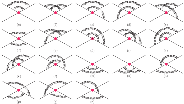
Figure 2: The Feynman graphs for the NNLO QCD corrections to the operator ${\mathcal{O}}(^{3}S^{[8]}_{1})$. We suppress the graphs which do not give rise to operator mixing with ${\mathcal{O}}(^{3}S^{[1]}_{1})$.

We proceed to deal with the NNLO QCD corrections to the operator ${\mathcal{O}}(^{3}S^{[8]}_{1})$. The relevant Feynman graphs are illustrated in Fig. 2. There are totally eighteen Feynman graphs which do contribution. We are able to project out the color-singlet contribution by employing the color decompositions

$$T^{a}T^{b}T^{c}\otimes T^{a}T^{b}T^{c} = \frac{-2}{27}\,1\otimes 1+{\rm others},$$ (39a)

$$T^{a}T^{b}T^{c}\otimes T^{b}T^{a}T^{c} = \frac{7}{27}\,1\otimes 1+{\rm others},$$ (39b)

where we merely keep the color-singlet part. Through simple analysis, we find the color factors are $\frac{7}{27}\,1\otimes 1$ for the diagrams Fig. 2(a,e-g,i,k,m,p,q) and $-\frac{2}{27}\,1\otimes 1$ for the diagrams Fig. 2(b-d,h,j,l,n,o,r).

With the Feynman rules, the amplitude of Fig. 2(a) reads

$$I_{2a} = \frac{(ig_{s})^{4}}{16m^{4}}\int\!\!\frac{d^{d}k}{(2\pi)^{d}}\int\!\!\frac{d^{d}l}{(2\pi)^{d}}\frac{i}{p^{0}-k^{0}-\frac{(\vec{{\bm{p}}}-\vec{{\bm{k}}})^{2}}{2m}+i\epsilon}\frac{i}{p^{\prime 0}-k^{0}-\frac{(\vec{{\bm{p}}^{\prime}}-\vec{{\bm{k}}})^{2}}{2m}+i\epsilon}$$ (40)

$$\times\frac{i}{p^{0}-k^{0}-l^{0}-\frac{(\vec{{\bm{p}}}-\vec{{\bm{k}}}-\vec{{\bm{l}}})^{2}}{2m}+i\epsilon}\frac{i}{p^{\prime 0}-k^{0}-l^{0}-\frac{(\vec{{\bm{p}}^{\prime}}-\vec{{\bm{k}}}-\vec{{\bm{l}}})^{2}}{2m}+i\epsilon}$$

$$\times\frac{4i({\bm{p}}\cdot{\bm{p}}^{\prime}-{\bm{p}}\cdot{\bm{k}}{\bm{p}}^{\prime}\cdot{\bm{k}}/{\bm{k}}^{2})}{k^{2}+i\epsilon}\frac{4i[({\bm{p}}-{\bm{k}})\cdot({\bm{p}}^{\prime}-{\bm{k}})-({\bm{p}}-{\bm{k}})\cdot{\bm{l}}({\bm{p}}^{\prime}-{\bm{k}})\cdot{\bm{l}}/{\bm{l}}^{2}]}{l^{2}+i\epsilon}$$

$$= \frac{g_{s}^{4}}{4m^{4}}\frac{(d-2)^{2}}{(d-1)^{2}}\int\!\!\frac{d^{d-1}k}{(2\pi)^{d-1}}\int\!\!\frac{d^{d-1}l}{(2\pi)^{d-1}}\frac{({\bm{p}}\cdot{\bm{p}}^{\prime})^{2}}{|{\bm{k}}|^{3}|{\bm{l}}|(|{\bm{k}}|+|{\bm{l}}|)^{2}},$$

where the color factor is suppressed.

Analogous to (40), we are able to get all others

$$I_{2b} = \frac{g_{s}^{4}}{4m^{4}}\frac{(d-2)^{2}}{(d-1)^{2}}\int\!\!\frac{d^{d-1}k}{(2\pi)^{d-1}}\int\!\!\frac{d^{d-1}l}{(2\pi)^{d-1}}\frac{({\bm{p}}\cdot{\bm{p}}^{\prime})^{2}}{|{\bm{k}}|^{2}|{\bm{l}}|^{2}(|{\bm{k}}|+|{\bm{l}}|)^{2}},$$

$$I_{2c} = \frac{g_{s}^{4}}{4m^{4}}\frac{(d-2)^{2}}{(d-1)^{2}}\int\!\!\frac{d^{d-1}k}{(2\pi)^{d-1}}\int\!\!\frac{d^{d-1}l}{(2\pi)^{d-1}}\frac{({\bm{p}}\cdot{\bm{p}}^{\prime})^{2}}{|{\bm{k}}|^{3}|{\bm{l}}|^{2}(|{\bm{k}}|+|{\bm{l}}|)},$$

$$I_{f} = \frac{g_{s}^{4}}{4m^{4}}\frac{(d-2)^{2}}{(d-1)^{2}}\int\!\!\frac{d^{d-1}k}{(2\pi)^{d-1}}\int\!\!\frac{d^{d-1}l}{(2\pi)^{d-1}}\frac{({\bm{p}}\cdot{\bm{p}}^{\prime})^{2}}{|{\bm{k}}|^{3}|{\bm{l}}|^{3}},$$

$$I_{h} = I_{j}=I_{m}=I_{a},$$

$$I_{i} = I_{k}=I_{n}=I_{b},$$

$$I_{d} = I_{e}=I_{g}=I_{o}=I_{p}=I_{q}=I_{r}=I_{c},$$

$$I_{l} = I_{f}.$$ (41)

Including the color factors, and summing over all these contributions, we get

$$I = \frac{5}{54}\frac{2g_{s}^{4}}{m^{4}}\frac{(d-2)^{2}}{(d-1)^{2}}\,1\otimes 1\int\!\!\frac{d^{d-1}k}{(2\pi)^{d-1}}\int\!\!\frac{d^{d-1}l}{(2\pi)^{d-1}}\frac{({\bm{p}}\cdot{\bm{p}}^{\prime})^{2}}{|{\bm{k}}|^{3}|{\bm{l}}|^{3}}$$ (42)

$$= \frac{20\alpha_{s}^{2}}{243\pi^{2}(d-1)}\frac{{\bm{p}}^{4}}{m^{4}}\bigg{(}\frac{\tilde{f}_{\epsilon}}{\epsilon_{\rm UV}}-\frac{\tilde{f}_{\epsilon}}{\epsilon_{\rm IR}}\bigg{)}^{2}1\otimes 1,$$

where we use ${{\bm{p}}^{\prime}}^{2}={\bm{p}}^{2}$.

In addition, we also need to calculate the NLO QCD corrections to the counterterm $\delta_{1}{\mathcal{O}}$. Employing (37), we readily obtain

$$\delta_{1}{\mathcal{O}}^{(1)} = -\frac{5\alpha_{s}}{9\pi m^{2}}\frac{\tilde{f}_{\epsilon}}{\epsilon_{\rm UV}}\sum_{J}{\mathcal{O}}(^{3}P^{[8]}_{J})^{(1)}=-\frac{40\alpha_{s}^{2}}{243\pi^{2}(d-1)}\frac{{\bm{p}}^{4}}{m^{4}}\frac{\tilde{f}_{\epsilon}}{\epsilon_{\rm UV}}\bigg{(}\frac{\tilde{f}_{\epsilon}}{\epsilon_{\rm UV}}-\frac{\tilde{f}_{\epsilon}}{\epsilon_{\rm IR}}\bigg{)}{\mathcal{O}}(^{3}S^{[1]}_{1}).\phantom{x}$$ (43)

Combining (42) and (43), we get

$${\mathcal{O}}(^{3}S^{[8]}_{1})^{(2)} = \frac{20\alpha_{s}^{2}}{243\pi^{2}}\frac{{\bm{p}}^{4}}{(d-1)m^{4}}\bigg{(}-\frac{\tilde{f}_{\epsilon}^{2}}{\epsilon_{\rm UV}^{2}}+\frac{\tilde{f}_{\epsilon}^{2}}{\epsilon_{\rm IR}^{2}}\bigg{)}{\mathcal{O}}(^{3}S^{[1]}_{1})+\delta_{2}{\mathcal{O}},$$ (44)

where the UV divergence can be canceled through the counterterm. Finally, we present the renormalized operator and the corresponding counterterm

$${\mathcal{O}}(^{3}S^{[8]}_{1})_{\overline{\rm MS}} = {\mathcal{O}}(^{3}S^{[8]}_{1})^{(0)}-\frac{5\alpha_{s}}{9\pi m^{2}}\frac{\tilde{f}_{\epsilon}}{\epsilon_{\rm IR}}\sum_{J}{\mathcal{O}}(^{3}P^{[8]}_{J})+\frac{20\alpha_{s}^{2}}{243\pi^{2}}\frac{{\bm{p}}^{4}}{(d-1)m^{4}}\frac{\tilde{f}_{\epsilon}^{2}}{\epsilon_{\rm IR}^{2}}{\mathcal{O}}(^{3}S^{[1]}_{1}),$$ (45a)

$$\delta_{2}{\mathcal{O}} = \frac{20\alpha_{s}^{2}}{243\pi^{2}}\frac{{\bm{p}}^{4}}{(d-1)m^{4}}\frac{\tilde{f}_{\epsilon}^{2}}{\epsilon_{\rm UV}^{2}}{\mathcal{O}}(^{3}S^{[1]}_{1}).$$ (45b)

IV.2 $P$-wave color-octet

In this subsection, we determine the short-distance coefficients $dF({}^{3}P^{[8]}_{J})$ through calculating the decay rates of the perturbative processes $b\bar{b}(^{3}P^{[8]}_{J})\to c\bar{c}g$. The factorization formulas for these processes are expressed as

$$d\Gamma(^{3}P^{[8]}_{J}) = \frac{dF(^{3}P^{[8]}_{J})}{m^{4}}\langle{\mathcal{O}}(^{3}P^{[8]}_{J})\rangle_{b\bar{b}(^{3}P^{[8]}_{J})}+\frac{dF(^{3}S^{[8]}_{1})}{m^{2}}\langle{\mathcal{O}}(^{3}S^{[8]}_{1})\rangle_{b\bar{b}(^{3}P^{[8]}_{J})}.$$ (46)

We can utilize (25) to calculate the decay rates in full QCD. First, we need to obtain $H(^{3}P^{[8]}_{J})$ defined in (26). To understand the IR structure and show the IR cancelation, here we separate $H(^{3}P^{[8]}_{J})$ into two parts: $H(^{3}P^{[8]}_{J})=H_{d}(^{3}P^{[8]}_{J})+H_{s}(^{3}P^{[8]}_{J})$. $H_{d}(^{3}P^{[8]}_{J})$ include the terms proportional to $1/(1-z)$, which contribute the whole IR divergences to the decay rates from the region with the real gluon being soft. $H_{s}(^{3}P^{[8]}_{J})$ take in charge of the remainder, which is absent of any singularity. Correspondingly, we use the subscripts $d$, $s$ in both $d\Gamma(^{3}P^{[8]}_{J})$ and $dF(^{3}P^{[8]}_{J})$ to denote the contributions from the two parts. The advantage of this classification will be recognized when we determine the short-distance coefficient $dF(^{3}S^{[1]}_{1})$.

IV.2.1 $H_{d}(^{3}P_{J}^{[8]})$

We directly present the expressions of $H_{d}(^{3}P^{[8]}_{J})$

$$H_{d}({}^{3}P^{[8]}_{J}) = \frac{5\alpha_{s}^{2}(1-\epsilon){\bm{p}}^{2}}{3m^{4}(1-z)(3-2\epsilon)},$$ (47)

which are the same for $J=0,1,2$.

It is useful to make the following expansion

$$\frac{1}{(1-z)^{1+2\epsilon}}=-\frac{(1-r)^{-2\epsilon}}{2\epsilon}\delta(1-z)+\bigg{(}\frac{1}{1-z}\bigg{)}_{+}-2\epsilon\bigg{(}\frac{\ln(1-z)}{1-z}\bigg{)}_{+}+{\mathcal{O}}(\epsilon^{2}),$$ (48)

where the plus functions are defined via

$$\int_{r}^{1}\!\!dz(a)_{+}f(z)\equiv\int_{r}^{1}\!\!dza\bigg{[}f(z)-f(1)\bigg{]}.$$ (49)

Inserting (47) into (25) and employing (48), we are able to get the differential decay rates $d\Gamma_{d}({}^{3}P^{[8]}_{J})$, which embrace IR divergences. Incorporating the factorization formulas (46) and the expressions (31) and (36a), we find the IR divergences appearing on the left hand side of (46) are exactly canceled by the renormalized $S$-wave color-octet matrix element on the right hand side. It renders the short-distance coefficients $dF(^{3}P^{[8]}_{J})$ free of any singularity:

$$\frac{dF_{d}(^{3}P^{[8]}_{J})}{dz} = -\frac{5\alpha_{s}^{2}Lf_{\epsilon}}{18}\bigg{\{}\bigg{[}\frac{1}{\epsilon_{\rm IR}}\bigg{(}1-\frac{\tilde{f}_{\epsilon}}{f_{\epsilon}}\bigg{)}+\frac{5}{3}-2\ln(1-r)+\bigg{(}2\ln^{2}(1-r)-\frac{10}{3}\ln(1-r)$$ (50)

$$-\frac{\pi^{2}}{4}+\frac{28}{9}\bigg{)}\epsilon\bigg{]}\delta(1-z)-\bigg{(}\frac{1}{1-z}\bigg{)}_{+}\bigg{[}2+\frac{10\epsilon}{3}\bigg{]}+4\epsilon\bigg{(}\frac{\ln(1-z)}{1-z}\bigg{)}_{+}\bigg{\}}.$$

In (50), we keep the terms linearly dependent on $\epsilon$, which will induce finite contributions to the short-distance coefficient $dF(^{3}S^{[1]}_{1})$.

IV.2.2 $H_{s}({}^{3}P^{[8]}_{J})$

We present the expressions of $H_{s}({}^{3}P^{[8]}_{J})$ as

$$H_{s}({}^{3}P^{[8]}_{0}) = \frac{5\alpha_{s}^{2}(5-z)(1-\epsilon){\bm{p}}^{2}}{12m^{4}(3-2\epsilon)},$$ (51a)

$$H_{s}({}^{3}P^{[8]}_{1}) = -\frac{5\alpha_{s}^{2}[2+z-2(1+z)\epsilon]{\bm{p}}^{2}}{6m^{4}(3-2\epsilon)},$$ (51b)

$$H_{s}({}^{3}P^{[8]}_{2}) = -\frac{5\alpha_{s}^{2}[4+z-(1+z)\epsilon]{\bm{p}}^{2}}{6m^{4}(15-16\epsilon+4\epsilon^{2})}.$$ (51c)

The corresponding differential decay rates can be achieved by multiplying a constant factor:

$$\frac{dF_{s}(^{3}P^{[8]}_{0})}{dz} = \frac{5(5-z)\alpha_{s}^{2}Lf_{\epsilon}}{36}\bigg{[}1-2\epsilon\ln(1-z)+\frac{5\epsilon}{3}\bigg{]},$$ (52a)

$$\frac{dF_{s}(^{3}P^{[8]}_{1})}{dz} = -\frac{5\alpha_{s}^{2}Lf_{\epsilon}}{18}\bigg{[}z+2-2\epsilon(z+2)\ln(1-z)+\frac{2(z+5)}{3}\epsilon\bigg{]},$$ (52b)

$$\frac{dF_{s}(^{3}P^{[8]}_{2})}{dz} = -\frac{\alpha_{s}^{2}Lf_{\epsilon}}{18}\bigg{[}z+4-2\epsilon(z+4)\ln(1-z)+\frac{1}{15}(31z+169)\epsilon\bigg{]}.$$ (52c)

IV.3 $S$-wave color-singlet

In this section, we determine the short-distance coefficient $dF({}^{3}S^{[1]}_{1})$ through calculating the decay rate of the process $b\bar{b}({}^{3}S^{[1]}_{1})\to c\bar{c}gg$. The corresponding factorization formula is expressed as

$$d\Gamma({}^{3}S^{[1]}_{1}) = \frac{dF_{1}({}^{3}S^{[1]}_{1})}{m^{2}}\langle\mathcal{O}({}^{3}S^{[1]}_{1})\rangle_{H}+\frac{dF_{2}({}^{3}S^{[1]}_{1})}{m^{4}}\langle\mathcal{P}({}^{3}S^{[1]}_{1})\rangle_{H}$$ (53)

$$+\frac{dF_{3}({}^{3}S^{[1]}_{1})}{m^{6}}\langle\mathcal{Q}_{1}({}^{3}S^{[1]}_{1})\rangle_{H}+\frac{dF_{4}({}^{3}S^{[1]}_{1})}{m^{6}}\langle\mathcal{Q}_{2}({}^{3}S^{[1]}_{1})\rangle_{H}$$

$$+\frac{dF({}^{3}S^{[8]}_{1})}{m^{2}}\langle\mathcal{O}({}^{3}S^{[8]}_{1})\rangle_{H}+\sum_{J}\frac{dF({}^{3}P^{[8]}_{J})}{m^{4}}\langle\mathcal{O}({}^{3}P^{[8]}_{J})\rangle_{H},$$

where the subscript ‘$H$’ in the matrix elements represents $b\bar{b}({}^{3}S^{[1]}_{1})$. As mentioned in Sec. II, the two matrix elements in the second line of (53) are equal at relative order $v^{4}$. Therefore, we will determine the combined short-distance coefficient $dF({}^{3}S^{[1]}_{1})$ defined in (5) in this subsection.

There are six diagrams for this process. The formula for the decay rate is given in (20). Firstly, we need to calculate $H(^{3}S^{[1]}_{1})$, which is defined in (21). To separate the relativistic corrections , we expand $H(^{3}S^{[1]}_{1})$ in powers of ${\bm{p}}^{2}$:

$$H(^{3}S^{[1]}_{1})=H^{(0)}(^{3}S^{[1]}_{1})+H^{(2)}(^{3}S^{[1]}_{1})\frac{{\bm{p}}^{2}}{m^{2}}+H^{(4)}(^{3}S^{[1]}_{1})\frac{{\bm{p}}^{4}}{m^{4}}+{\cal O}({\bm{p}}^{6}),$$ (54)

where the first two orders have been considered in Ref. Chen:2011ph . Our remainder task is to calculate $H^{(4)}(^{3}S^{[1]}_{1})$ and the corresponding decay rate. At order $v^{4}$, the decay rate involves IR divergences. Analogous to the treatment in the previous subsection, we separate $H^{(4)}(^{3}S^{[1]}_{1})$ into three parts: $H^{(4)}(^{3}S^{[1]}_{1})=H^{(4)}_{d}(^{3}S^{[1]}_{1})+H^{(4)}_{s}(^{3}S^{[1]}_{1})+H^{(4)}_{r}(^{3}S^{[1]}_{1})$. $H^{(4)}_{d}(^{3}S^{[1]}_{1})$ proportional to $1/(1-z)$ contributes the whole IR divergences to the decay rate in the region where the two real gluons are simultaneous soft. In the following, we will demonstrate that the IR divergences can be thoroughly canceled by the renormalized $S$-wave color-octet matrix element (45a) with the short-distance coefficient (31), together with the renormalized $P$-wave matrix elements (38) with the short-distance coefficients $dF_{d}(^{3}P^{[8]}_{J})$ given in (50). $H^{(4)}_{s}(^{3}S^{[1]}_{1})$ contributes the whole IR divergence to the decay rate in the region where only one of the real gluons is soft, as a result, it should be proportional to either $1/x$ or $1/(1-x)$. We will show that the IR divergence can be thoroughly canceled by the renormalized $P$-wave matrix elements (38) with short-distance coefficients $dF_{s}(^{3}P^{[8]}_{J})$ given in (52). $H^{(4)}_{r}(^{3}S^{[1]}_{1})$ takes in charge of the remainder and therefore corresponds to a finite contribution to the decay rate. Similarly, we use the subscripts $d$, $s$, $r$ in both $d\Gamma(^{3}S^{[1]}_{1})$ and $dF(^{3}S^{[1]}_{1})$ to denote the contributions from the three parts.

IV.3.1 $H^{(4)}_{d}(^{3}S^{[1]}_{1})$

In this subsection, we calculate the decay rate and short-distance coefficient related to $H^{(4)}_{d}(^{3}S^{[1]}_{1})$. First, we present the expression

$$H^{(4)}_{d}(^{3}S^{[1]}_{1})=\frac{40\alpha_{s}^{3}}{243m^{2}\pi x(1-x)(1-z)}\bigg{[}3(2y^{2}-2y+1)+(8y^{2}-8y+1)\epsilon-8y(1-y)\epsilon^{2}\bigg{]}.\phantom{x}$$ (55)

This term is proportional to $1/(1-z)$. In addition, we notice it also contains the factor $1/x(1-x)$. Therefore, we expect it will contribute a double IR pole to the decay rate at the endpoints of $z$ and $x$.

Employing the expansion

$$\frac{1}{(1-z)^{1+4\epsilon}}=-\frac{(1-r)^{-4\epsilon}}{4\epsilon}\delta(1-z)+\bigg{(}\frac{1}{1-z}\bigg{)}_{+}-4\epsilon\bigg{(}\frac{\ln(1-z)}{1-z}\bigg{)}_{+}+{\mathcal{O}}(\epsilon^{2}),$$ (56)

and integrating out the variables $x,y$, we are able to obtain the differential decay rate

$$\frac{d\Gamma_{d}({}^{3}S^{[1]}_{1})}{dz} = \frac{20\alpha_{s}^{3}Lf_{\epsilon}^{2}{\bm{p}}^{4}}{243\pi m^{6}}\bigg{\{}\bigg{[}\frac{1}{\epsilon^{2}}+\frac{4-4\ln(1-r)}{\epsilon}+8\ln^{2}(1-r)-16\ln(1-r)-\frac{7\pi^{2}}{6}+\frac{35}{3}\bigg{]}$$ (57)

$$\times\delta(1-z)-\bigg{(}\frac{1}{1-z}\bigg{)}_{+}\bigg{[}\frac{4}{\epsilon}+2\ln z+16\bigg{]}+16\bigg{(}\frac{\ln(1-z)}{1-z}\bigg{)}_{+}\bigg{\}}.$$

Inserting (57) into the factorization formula (53), we see the IR divergences on the left hand side are exactly canceled by the $S$-wave color-octet contribution, together with the renormalized $P$-wave color-octet matrix elements with the short-distance coefficients $dF_{d}(^{3}P^{[8]}_{J})$ on the right hand side. Straightforwardly, we get

$$\frac{dF_{d}(^{3}S^{[1]}_{1})}{dz} = \frac{10\alpha_{s}^{3}L}{729\pi}\bigg{\{}\bigg{[}\ln^{2}\!\!\frac{\mu^{2}}{M^{2}}+\frac{10-12\ln(1-r)}{3}\ln\!\frac{\mu^{2}}{M^{2}}+4\ln^{2}(1-r)-\frac{20}{3}\ln(1-r)+\frac{25}{9}$$ (58)

$$-\frac{2\pi^{2}}{3}\bigg{]}\delta(1-z)-\bigg{(}\frac{1}{1-z}\bigg{)}_{+}\bigg{[}4\ln\!\frac{\mu^{2}}{M^{2}}+2\ln z+\frac{20}{3}\bigg{]}+8\bigg{(}\frac{\ln(1-z)}{1-z}\bigg{)}_{+}\bigg{\}},$$

where $\mu$ indicates the factorization scale.

IV.3.2 $H^{(4)}_{s}(^{3}S^{[1]}_{1})$

The expression of $H^{(4)}_{s}(^{3}S^{[1]}_{1})$ reads

$$H^{(4)}_{s}(^{3}S^{[1]}_{1}) = \frac{20\alpha_{s}^{3}}{243\pi m^{2}}\bigg{\{}\frac{-8y^{2}+8y-z-3}{x}+\frac{2(z-5)(y^{2}-y)+z-1}{x}\epsilon-\frac{1}{(1-y+yz)^{4}}$$ (59)

$$\times\frac{1}{1-x}\bigg{[}12(1-z)^{3}y^{6}+12(z-5)(z-1)^{2}y^{5}-6(z^{3}-11z^{2}+31z-21)y^{4}$$

$$-24(z^{2}-5z+6)y^{3}+(z^{4}+z^{3}+9z^{2}-27z+96)y^{2}+2(z^{3}-2z^{2}-3z-18)y$$

$$+z^{2}+3z+6+\epsilon\bigg{(}16(1-z)^{3}y^{6}+16(z-5)(z-1)^{2}y^{5}-2(z-1)$$

$$\times(z^{2}-34z+81)y^{4}-8(z^{2}-14z+21)y^{3}-(z^{4}-z^{3}-9z^{2}-3z-92)y^{2}$$

$$-2(3z^{2}+7z+12)y-z^{2}+z+2\bigg{)}\bigg{]}\bigg{\}}.$$

This term is proportional to either $1/x$ or $1/(1-x)$, therefore, it contributes single poles to the decay rate at the endpoints of $x$, i.e., $x\to 0$ and $x\to 1$. After integrating out the variables $x,y$, we have

$$\frac{d\Gamma_{s}(^{3}S^{[1]}_{1})}{dz} = \frac{20\alpha_{s}^{3}Lf_{\epsilon}^{2}{\bm{p}}^{4}}{729\pi m^{6}}\bigg{\{}\frac{3z+5}{\epsilon}+\frac{1}{3(1-z)^{4}}\bigg{[}21z^{5}-43z^{4}-101z^{3}+291z^{2}-248z+80$$ (60)

$$+3(3z^{5}-4z^{4}+4z^{3}+12z^{2}-9z+6)\ln z\bigg{]}-4(3z+5)\ln(1-z)\bigg{\}}.$$

It is not hard to find that the IR divergence in (60) is exactly canceled by the renormalized $P$-wave color-octet matrix elements with the short-distance coefficients $dF_{s}({}^{3}P^{[8]}_{J})$, as we expected. We present the final result

$$\frac{dF_{s}(^{3}S^{[1]}_{1})}{dz} = \frac{10\alpha_{s}^{3}L}{2187\pi}\bigg{\{}(3z+5)\ln\!\frac{\mu^{2}}{M^{2}}+\frac{1}{3(1-z)^{4}}\bigg{[}6z^{5}-16z^{4}-59z^{3}+153z^{2}-131z+47$$ (61)

$$+3(3z^{5}-4z^{4}+4z^{3}+12z^{2}-9z+6)\ln z\bigg{]}-2(3z+5)\ln(1-z)\bigg{\}}.$$

IV.3.3 $H^{(4)}_{r}(^{3}S_{1}^{[1]})$

Finally, we deal with $H^{(4)}_{r}(^{3}S^{[1]}_{1})$, which will produce a finite contribution to the decay rate. Since the expression of $H^{(4)}_{r}(^{3}S^{[1]}_{1})$ is both tedious and cumbersome, here we merely present the differential short-distance coefficient as

$$\frac{dF_{r}({}^{3}S^{[1]}_{1})}{dz} = \frac{\alpha_{s}^{3}L}{262440\pi(1-z)^{4}}\bigg{\{}15{\rm tan}^{-1}\!\bigg{(}\sqrt{\frac{1-z}{z}}\bigg{)}\bigg{[}6(86z^{5}-279z^{4}-2548z^{3}+6718z^{2}$$ (62)

$$-5694z+1609){\rm tan}^{-1}\!\bigg{(}\sqrt{\frac{1-z}{z}}\bigg{)}+\sqrt{z(1-z)}(13908-38215z+33375z^{2}$$

$$-7296z^{3}-476z^{4})\bigg{]}-6(299z^{5}+22640z^{4}-27848z^{3}+16208z^{2}-2015z+700)$$

$$\times\ln z-(1-z)(68916z^{4}-256073z^{3}+696819z^{2}-669618z+229580)\bigg{\}}.\phantom{xxx}$$

IV.4 Summarizing the differential short-distance coefficients

We summarize the differential short-distance coefficients calculated in the above:

$$\frac{dF({}^{3}S^{[8]}_{1})}{dz} = \frac{\pi\alpha_{s}L}{2}\delta(1-z),$$ (63a)

$$\frac{dF(^{3}P^{[8]}_{J})}{dz} = \!\!\frac{-5\alpha_{s}^{2}L}{18}\bigg{\{}\bigg{[}\ln\!\frac{\mu^{2}}{M^{2}}+\frac{5}{3}-2\ln(1-r)\bigg{]}\delta(1-z)-2\bigg{(}\frac{1}{1-z}\bigg{)}_{+}+A_{J}\bigg{\}},$$ (63b)

$$\frac{dF(^{3}S^{[1]}_{1})}{dz} = \frac{dF_{d}(^{3}S^{[1]}_{1})}{dz}+\frac{dF_{s}(^{3}S^{[1]}_{1})}{dz}+\frac{dF_{r}(^{3}S^{[1]}_{1})}{dz},$$ (63c)

where $A_{J}$ are $-\tfrac{5-z}{2}$, $2+z$, and $\tfrac{4+z}{5}$ for $J=0,1,2$ respectively.

V Discussions and summaries

V.1 Discussions

Applying the formulas (63) for the differential short-distance coefficients obtained in the last section, we now make some discussions.

V.1.1 ${dF(^{3}S^{[1]}_{1})}/{dz}$ in the limit of $z\to 0$

We first discuss the short-distance coefficient $dF(^{3}S^{[1]}_{1})/dz$ in the limit of $z\to 0$. It is not hard to derive

$$\frac{1}{L}\frac{dF(^{3}S^{[1]}_{1})}{dz}\bigg{|}_{z\to 0}=-\frac{35\alpha_{s}^{3}}{2187\pi}\ln z-\frac{70\alpha_{s}^{3}}{2187\pi}\ln\!\frac{\mu^{2}}{M^{2}}+\frac{1609\pi\alpha_{s}^{3}}{11664}-\frac{3913\alpha_{s}^{3}}{4374\pi}.$$ (64)

In (64), we notice that the limitation bears the logarithmic divergence $\ln z$. It is no surprise, owing to the fact we actually do not regularize the singularity when $z$ approaches to 0. Moreover, we find that the coefficient of $\ln z$ equals exactly to the corresponding coefficient of IR divergence in the decay rate of the process $b\bar{b}(^{3}S^{[1]}_{1})\to 3g$ up to a factor $\frac{1}{2\pi}\times\frac{1}{2}$, as our expectation (The constant factor originates in from (15).). On the other hand, when either of the two real gluons becomes soft, there exists IR divergence which is regularized in dimensional regularization and canceled by the renormalized $P$-wave color-octet matrix elements. The term proportional to $\ln\!\frac{\mu^{2}}{M^{2}}$ is related to the divergence. We are delight with that the coefficient of $\ln\!\frac{\mu^{2}}{M^{2}}$ is exactly double that of $\ln z$.

V.1.2 Color-singlet differential short-distance coefficients

In (63), the two types of plus functions $(\tfrac{1}{1-z})_{+}$ and $(\tfrac{\ln(1-z)}{1-z})_{+}$ diverge as $z\to 1$. Since these singularities arise when the momenta of the real gluons in the final states go to 0, the distributions are actually unreliable in this region. Nevertheless, the singularities in the distributions are smeared when one integrates out $z$ and so the integrated short-distance coefficients are well behaved. In order to investigate the dependence of the relativistic corrections on the virtuality of the intermediate gluon, it is intriguing and enlightening to study two ratios: $t_{1}(z)\equiv dF_{2}(^{3}S^{[1]}_{1})/dF_{1}(^{3}S^{[1]}_{1})$ and $t_{2}(z)\equiv dF(^{3}S^{[1]}_{1})/dF_{1}(^{3}S^{[1]}_{1})$, where $dF_{1}(^{3}S^{[1]}_{1})$ and $dF_{2}(^{3}S^{[1]}_{1})$ are defined in (1) and have been obtained in (53) of Ref. Chen:2011ph .

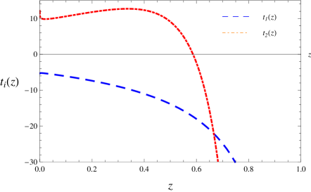
Figure 3: Ratios of the differential short-distance coefficients. The blue dashed line represents the distribution $t_{1}(z)$, while the red dot-dashed line represents the distribution $t_{2}(z)$. We specify the factorization scale $\mu=M$ in $t_{2}(z)$.

To see it clearly, we plot Fig. 3 to illustrate the two ratios. In the figure, we observe that $t_{1}(z)$ which reflects the NLO relativistic corrections is negative and its magnitude rises quickly with increase of the virtuality of the immediate gluon. However $t_{2}(z)$ which reflects the order-$v^{4}$ relativistic corrections is positive in small values of $z$ and turns to negative in large values. The magnitude of $t_{2}(z)$ is sizable in most values of $z$.

V.1.3 Integrated color-singlet short-distance coefficients

Finally, we integrate out the variable $z$ and investigate the integrated short-distance coefficients. In Table. 1, we list the ratios of the order-$v^{2}$ and the order-$v^{4}$ color-singlet short-distance coefficients to the LO one for the processes of $\Upsilon(nS)$ inclusive decay into a charm pair.

Table 1: Ratios of the short-distance coefficients for $\Upsilon\to c\bar{c}gg$. The charm mass is selected to that of the $D$ meson Kang:2007uv ; Chen:2011ph . The masses of the $D$ meson and bottomonia are taken from Ref. Nakamura:2010zzi .

	$r$	$F_{2}(^{3}S^{[1]}_{1})/F_{1}(^{3}S^{[1]}_{1})$	$F(^{3}S^{[1]}_{1})/F_{1}(^{3}S^{[1]}_{1})$
$\Upsilon(1S)$	$1.56\times 10^{-1}$	$-12.4$	$19.4+0.6\ln^{2}(\frac{\mu^{2}}{M^{2}})+0.9\ln(\frac{\mu^{2}}{M^{2}})$
$\Upsilon(2S)$	$1.39\times 10^{-1}$	$-11.7$	$18.5+0.5\ln^{2}(\frac{\mu^{2}}{M^{2}})+0.6\ln(\frac{\mu^{2}}{M^{2}})$
$\Upsilon(3S)$	$1.30\times 10^{-1}$	$-11.4$	$18.0+0.5\ln^{2}(\frac{\mu^{2}}{M^{2}})+0.4\ln(\frac{\mu^{2}}{M^{2}})$

We learn from the table that the ratio $F(^{3}S^{[1]}_{1})/F_{1}(^{3}S^{[1]}_{1})$ is both positive and sizable, nevertheless, the relativistic expansion is of well convergence due to a small value of $v$ (e.g., $v^{2}\sim 0.1$.). The situation is quite similar to the case for the process $J/\psi\to ggg$ Bodwin:2002hg . To further study the relation between the relativistic corrections and $r$, we extrapolate the value of $r$ and investigate the ratios: $g_{1}(r)\equiv F_{2}(^{3}S^{[1]}_{1})(r)/F_{1}(^{3}S^{[1]}_{1})(r)$ and $g_{2}(r)\equiv F(^{3}S^{[1]}_{1})(r)/F_{1}(^{3}S^{[1]}_{1})(r)$. We illustrate the two functions in Fig. 4.

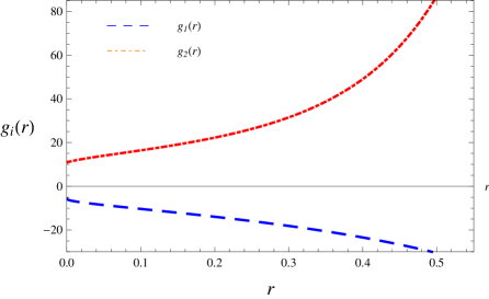
Figure 4: Ratios of the short-distance coefficients as functions of $r$. The blue dashed line represents the distribution $g_{1}(r)$, while the red dot-dashed line represents the distribution $g_{2}(r)$. We specify the factorization scale $\mu=M$ in $g_{2}(r)$.

From the figure, we find the NNLO relativistic corrections become more and more important with $r$ increase.

V.2 Summaries

In this work, we determine the short-distance coefficients within the framework of NRQCD factorization formula for $\Upsilon$ inclusive decay into a charm pair through relative order $v^{4}$. The order-$v^{4}$ color-singlet differential short-distance coefficient $dF(^{3}S^{[1]}_{1})$ is obtained through matching the decay rate of $b\bar{b}(^{3}S^{[1]}_{1})\to c\bar{c}gg$ in full QCD to that in NRQCD. The double and single IR divergences appearing in the decay rate are exactly canceled through the NNLO renormalization of the operator ${\mathcal{O}}(^{3}S^{[8]}_{1})$ and the NLO renormalization of the operators ${\mathcal{O}}(^{3}P^{[8]}_{J})$. To investigate the magnitude of the relativistic corrections and the convergence of the relativistic expansion, we show both the ratios of the differential short-distance coefficients $t_{i}(z)$ and the ratios of the short-distance coefficients $g_{i}(r)$. Our results indicate that though $F(^{3}S^{[1]}_{1})$ is quite large, the relativistic expansion from the color-singlet contributions in the process $\Upsilon\to c\bar{c}+X$ are well convergent due to a small value of $v$. In addition, we extrapolate $g_{i}(r)$ to a large range of $r$, and find the relativistic corrections rise quickly with increase of $r$.

References

• (1) G. T. Bodwin, E. Braaten and G. P. Lepage, Phys. Rev.  D 51, 1125 (1995) [Erratum-ibid.  D 55, 5853 (1997)] [arXiv:hep-ph/9407339].
• (2) E. Braaten and J. Lee, Phys. Rev. D 67, 054007 (2003) [Erratum-ibid. D 72, 099901 (2005)] [hep-ph/0211085].
• (3) Z. -G. He, Y. Fan and K. -T. Chao, Phys. Rev. D 75, 074011 (2007) [hep-ph/0702239 [HEP-PH]].
• (4) W. -L. Sang, R. Rashidin, U-R. Kim and J. Lee, Phys. Rev. D 84, 074026 (2011) [arXiv:1108.4104 [hep-ph]].
• (5) W. -Y. Keung and I. J. Muzinich, Phys. Rev. D 27, 1518 (1983).
• (6) H. -T. Chen, Y. -Q. Chen and W. -L. Sang, Phys. Rev. D 85, 034017 (2012) [arXiv:1109.6723 [hep-ph]].
• (7) H. -T. Chen, W. -L. Sang and P. Wu, Commun. Theor. Phys.  57, 665 (2012).
• (8) G. T. Bodwin, D. Kang, T. Kim, J. Lee and C. Yu, AIP Conf. Proc.  892, 315 (2007) [hep-ph/0611002].
• (9) G. T. Bodwin, J. Lee and C. Yu, Phys. Rev. D 77, 094018 (2008) [arXiv:0710.0995 [hep-ph]].
• (10) G. T. Bodwin and A. Petrelli, Phys. Rev. D 66, 094011 (2002) [hep-ph/0205210].
• (11) Hee Sok Chung, June-Haak Ee, Jungil Lee and Wen-Long Sang, work in progress.
• (12) G. T. Bodwin, U-R. Kim and J. Lee, arXiv:1208.5301 [hep-ph].
• (13) E. Braaten and Y. -Q. Chen, Phys. Rev. D 55, 2693 (1997) [hep-ph/9610401].
• (14) E. Braaten and Y. -Q. Chen, Phys. Rev. D 55, 7152 (1997) [hep-ph/9701242].
• (15) G. T. Bodwin, S. Kim and D. K. Sinclair, Nucl. Phys. Proc. Suppl.  34, 434 (1994). G. T. Bodwin, D. K. Sinclair and S. Kim, Phys. Rev. Lett.  77, 2376 (1996) [arXiv:hep-lat/9605023].
• (16) E. J. Eichten and C. Quigg, Phys. Rev. D 52, 1726 (1995) [hep-ph/9503356]. G. T. Bodwin, D. Kang, T. Kim, J. Lee and C. Yu, in Quark Confinement and the Hadron Spectrum VII: 7th Conference on Quark Confinement and the Hadron Spectrum-QCHS7, edited by J. Emilio, F. T. Ribeiro, N. Brambilla, A. Vairo, K. Maung, and G. M. Prosperi, AIP Conf. Proc.  892 (AIP, New York, 2007), p. 315 [arXiv:hep-ph/0611002]. Y. Q. Ma, K. Wang and K. T. Chao, Phys. Rev. Lett.  106, 042002 (2011) [arXiv:1009.3655 [hep-ph]].
• (17) H. -K. Guo, Y. -Q. Ma and K. -T. Chao, Phys. Rev. D 83, 114038 (2011) [arXiv:1104.3138 [hep-ph]].
• (18) G. T. Bodwin, H. S. Chung, D. Kang, J. Lee and C. Yu, Phys. Rev.  D 77, 094017 (2008) [arXiv:0710.0994 [hep-ph]].
• (19) Y. -J. Zhang and K. -T. Chao, Phys. Rev. D 78, 094017 (2008) [arXiv:0808.2985 [hep-ph]].
• (20) H. Fritzsch and K. H. Streng, Phys. Lett.  B 77 (1978) 299.
• (21) A. Y. Parkhomenko and A. D. Smirnov, Mod. Phys. Lett.  A 9, 115 (1994) [arXiv:hep-ph/9404260].
• (22) D. Kang, T. Kim, J. Lee and C. Yu, Phys. Rev.  D 76, 114018 (2007) [arXiv:0707.4056 [hep-ph]].
• (23) H. S. Chung, T. Kim and J. Lee, Phys. Rev.  D 78, 114027 (2008) [arXiv:0805.1989 [hep-ph]].
• (24) N. Brambilla, E. Mereghetti and A. Vairo, Phys. Rev. D 79, 074002 (2009) [Erratum-ibid. D 83, 079904 (2011)] [arXiv:0810.2259 [hep-ph]].
• (25) N. Brambilla, E. Mereghetti and A. Vairo, JHEP 0608, 039 (2006) [Erratum-ibid.  1104, 058 (2011)] [hep-ph/0604190].
• (26) J. P. Ma and Q. Wang, Phys. Lett. B 537, 233 (2002) [hep-ph/0203082].
• (27) A. Petrelli, M. Cacciari, M. Greco, F. Maltoni and M. L. Mangano, Nucl. Phys. B 514, 245 (1998) [hep-ph/9707223].
• (28) M. Beneke, F. Maltoni and I. Z. Rothstein, Phys. Rev. D 59, 054003 (1999) [hep-ph/9808360].
• (29) G. T. Bodwin, E. Braaten, D. Kang and J. Lee, Phys. Rev. D 76, 054001 (2007) [arXiv:0704.2599 [hep-ph]].
• (30) Z. -G. He, Y. Fan and K. -T. Chao, Phys. Rev. D 81, 074032 (2010) [arXiv:0910.3939 [hep-ph]].
• (31) G. T. Bodwin and Y. -Q. Chen, Phys. Rev. D 60, 054008 (1999) [hep-ph/9807492].
• (32) K. Nakamura et al. [Particle Data Group], J. Phys. G 37, 075021 (2010).