Charge trapping in the system of interacting quantum dots

Abstract

We analyzed the localized charge dynamics in the system of $N$ interacting single-level quantum dots (QDs) coupled to the continuous spectrum states in the presence of Coulomb interaction between electrons within the dots. Different dots geometry and initial charge configurations were considered. The analysis was performed by means of Heisenberg equations for localized electrons pair correlators.

We revealed that charge trapping takes place for a wide range of system parameters and we suggested the QDs geometry for experimental observations of this phenomenon. We demonstrated significant suppression of Coulomb correlations with the increasing of QDs number. We found the appearance of several time scales with the strongly different relaxation rates for a wide range of the Coulomb interaction values.

I Introduction

Coupled quantum dots (QDs) are recently under numerous experimental Wiel ,Potok ,Hayashi and theoretical investigations Stafford ,Matveev ,Boese ,Kikoin0 ,Orellana ,Arseyev_1 ,Arseyev_2 due to their potential application in modern nanoscale devices dealing with quantum kinetics of individual localized states Arseyev_1 ,Arseyev_2 ,Stafford_1 ,Hazelzet ,Cota ,Contreras-Pulido ,Elste ,Kennes . The kinetic properties of coupled QDs (artificial molecules) Wiel are governed by the Coulomb interaction between the localized electrons Hayashi ,Arseyev_2 and depend strongly on the dots topology, which determines energy levels spacing and the coupling rates Kastner ,Beenakker ,Alhassid . During the last decade experimental technique gives possibility to create vertically aligned strongly interacting QDs with only one of them coupled to the continuous spectrum states Vamivakas ,Stinaff . This so-called side-coupled geometry gives an opportunity to analyze non-stationary effects in formation of various charge and spin configurations in the small size structures Kikoin0 ,Arseyev_2 . Lateral QDs are extremely tunable by means of individual electrical gates Kastner_1 ,Ashoori . This advantage reveals in the possibility of single electron localization in the system of several coupled dots Chan and charge states manipulations in the artificial molecules. Therefore lateral QDs are considered to be an ideal candidates for creation of an efficient charge traps. Previous studies demonstrated long-lived charge occupation trap states in a single QDs Kuno_1 ,Kuno_2 ,Hummon and single electron spin trapping Brum . Single electron trapping in the double dot system was performed in Pioro . The temperature of the trapped electron was measured and tunnel coupling energy was extracted by charge sensing measurements. A full configuration-interaction study on a square QD containing several electrons in the presence of an attractive impurity was performed in Pujari . Authors demonstrated that the impurity changes significantly the charge densities of the two-electron QD excited states. The effect of correlations was revealed in the enhancement of the charge densities localization within the dot. QDs were investigated theoretically by various methods such as Keldysh non-equilibrium Green-function formalism Keldysh , re-normalization group theory Kikoin , specific approach suggested by Coleman Coleman , spin-density-functional theory Reimann or quantum Monte-Carlo calculations Foulkes .

In this paper we consider charge relaxation in the system of $N$ interacting QDs with on-site Coulomb repulsion coupled to the reservoir (continuous spectrum states). The analysis was performed by means of Heisenberg equations for the localized electrons pair correlators. We demonstrated the presence of strong charge trapping effects for the lateral QDs geometry. We found that on-site Coulomb repulsion results in the significant changing of the localized charge relaxation and leads to the formation of several time ranges with strongly different values of the relaxation rates. We also pointed out the significant suppression of Coulomb correlations influence on the localized charge relaxation with the increasing of dots number.

II Theoretical model

Let us consider relaxation processes in the system of $N$ identical lateral QDs which are situated in the different space points and are connected only with the single-central QD by means of electron tunneling processes with the same tunneling transfer amplitudes $T$. We assume that the single particle level spacing in the dots is large than all other energy scales, so that only one spin-degenerate level within the QD spectrum is accessible ($\varepsilon_{0}$ in the $N$ identical dots and $\varepsilon$ in the central one). QD with energy level $\varepsilon$ is also connected with the continuous spectrum states. Moreover we take into account Coulomb interaction between the localized electrons within the dots ($U$-in the central one and $U_{0}$ in the surrounding dots). Hamiltonian of the system under investigation has the form:

$$\hat{H} = \varepsilon a_{\sigma}^{+}a_{\sigma}+\sum_{\sigma,j=1}^{N}\varepsilon_{0}b_{j\sigma}^{+}b_{j\sigma}+\sum_{\sigma,j=1}^{N}(Tb_{j\sigma}^{+}a_{\sigma}+Ta_{\sigma}^{+}b_{j\sigma})+$$ (1)

$$+ \varepsilon_{k}c_{k\sigma}^{+}c_{k\sigma}+\sum_{k,\sigma}T_{k}(c_{k\sigma}^{+}a_{\sigma}+a_{\sigma}^{+}c_{k\sigma})+$$

$$+ Un_{a\sigma}n_{a-\sigma}+U_{0}n_{j\sigma}n_{j-\sigma}\$$

$T_{k}$ - tunneling amplitude between the single-central dot and continuous spectrum states. We assume $T$ and $T_{k}$ to be independent of momentum and spin. By considering a constant density of states in the reservoir $\nu_{0}$ (which is not a function of energy), the tunneling coupling strength $\gamma$ is defined as $\gamma=\pi\nu_{0}T_{k}^{2}$.

$a_{\sigma}^{+}/a_{\sigma}$($b_{j\sigma}^{+}/b_{j\sigma}$)- electrons creation/annihilation operators in the central dot (in the $N$ surrounding QDs). $c_{k}^{+}/c_{k}$- electrons creation/annihilation operators in the continuous spectrum states ($k$) and $n_{a\sigma}(n_{j\sigma})$ are electron filling numbers in the dots.

We’ll at first analyze filling numbers relaxation processes in the case when on-site Coulomb repulsion is absent in the whole system ($U=U_{0}=0$). Let us assume that at the initial moment all charge density in the system is localized only in one of the $N$ QDs and has the value $n_{1}(0)=n_{0}$. The filling numbers time evolution can be analyzed by means of kinetic equations for bilinear combinations of Heisenberg operators $a_{\sigma}^{+}/a_{\sigma}$ and $b_{j\sigma}^{+}/b_{j\sigma}$:

$$b_{j\sigma}^{+}b_{j^{{}^{\prime}}\sigma}=G_{jj^{{}^{\prime}}}(t);a_{\sigma}^{+}a_{\sigma}=G_{aa}(t)$$

$$b_{j\sigma}^{+}a_{\sigma}=G_{ja}(t);a_{\sigma}^{+}b_{j\sigma}=G_{aj}(t)\$$ (2)

Localized charge time evolution can be obtained from the system of equations for the Green functions $G_{jj^{{}^{\prime}}}$, $G_{aj}$, $G_{ja}$ and $G_{aa}$:

$$i\frac{\partial}{\partial t}G_{jj^{{}^{\prime}}} = T\cdot G_{ja}-T\cdot G_{aj^{{}^{\prime}}}$$

$$i\frac{\partial}{\partial t}G_{aa} = \sum_{j^{{}^{\prime}}}(T\cdot G_{aj^{{}^{\prime}}}-T\cdot G_{j^{{}^{\prime}}a})-i2\gamma\cdot G_{aa}$$

$$i\frac{\partial}{\partial t}G_{aj} = -\Delta\cdot G_{aj}+T\cdot G_{aa}-\sum_{j^{{}^{\prime}}}T\cdot G_{j^{{}^{\prime}}j}-i\gamma\cdot G_{aj}$$

$$i\frac{\partial}{\partial t}G_{ja} = \Delta\cdot G_{ja}-T\cdot G_{aa}+\sum_{j^{{}^{\prime}}}T\cdot G_{jj^{{}^{\prime}}}-i\gamma\cdot G_{ja}$$

where $\Delta=\varepsilon-\varepsilon_{0}$ is the detuning between the energy levels in the dots.

System of equations (LABEL:system_0) can be re-written in the compact matrix form (symbol $[]$ means commutation):

$$i\frac{\partial}{\partial t}\widehat{G}=[\widehat{G},\widehat{A}]-i(\widehat{B}\widehat{G}+\widehat{G}\widehat{B})$$ (4)

where $\widehat{G}$ is the pair correlators matrix:

$$\hat{G}=\begin{pmatrix}G_{aa}&G_{a1}&\ldots&G_{aN}\\ G_{1a}&\ldots&\ldots&G_{1N}\\ \vdots&\vdots&\vdots&\vdots\\ G_{Na}&G_{N1}&\ldots&G_{NN}\\ \end{pmatrix}$$ (5)

and matrix $\widehat{A}$ has the following form:

$$\hat{A}=\begin{pmatrix}\Delta&T_{1}&\ldots&T_{N}\\ T_{1}^{*}&0&\ldots&0\\ \vdots&0&\ldots&0\\ T_{N}^{*}&0&\ldots&0\\ \end{pmatrix}$$ (6)

The tunneling coupling matrix $\widehat{B}$ has only one nonzero element $||B||_{11}=\gamma$.

The formal solution of the system (4) can be found with the help of evolution operator:

$$\widehat{G}(t)=e^{[{-\widehat{B}t+i\widehat{A}t}]}\widehat{G}(0)e^{[{\widehat{B}t-i\widehat{A}t}]}$$ (7)

Consequently the average value of filling numbers time evolution in the one of the $N$ QDs can be found from the following expression:

$$\langle n_{j}(t)\rangle=\widehat{G}_{jj}(t)=\sum_{a,b}[e^{{-\widehat{B}t+i\widehat{A}t}}]_{ja}\widehat{G}_{ab}(0)[e^{{\widehat{B}t-i\widehat{A}t}}]_{bj}$$ (8)

Due to the condition that initial charge is localized only in one QD with number $j$, the following initial conditions are fulfilled: $<n_{j\sigma}(0)>=G_{jj}(0)=n_{0}$, $<n_{a\sigma}(0)>=0$, $<n_{j^{{}^{\prime}}\sigma}(0)>=0$, if $j\neq j^{{}^{\prime}}$ and $G_{jj^{{}^{\prime}}}(0)=G_{aj}(0)=G_{ja}(0)=0$.

Let us analyze filling numbers time evolution in the central QD and in the dot with initial charge. Concerning initial conditions one can easily find the expressions for filling numbers relaxation:

$$n_{j\sigma}(t) = [e^{i\widehat{H}t}]_{jj}n_{0j}[e^{-i\widehat{\widetilde{H}}t}]_{jj}$$

$$n_{a\sigma}(t) = [e^{i\widehat{H}t}]_{aj}n_{0j}[e^{-i\widehat{\widetilde{H}}t}]_{ja}\$$ (9)

where operators $\widehat{H}=\widehat{A}+i\widehat{B}$ and $\widehat{\widetilde{H}}=\widehat{A}-i\widehat{B}$ are included. Further analysis deals with the calculation of matrix exponent’s elements. One can easily perform this procedure with the help of recurrent ratio similar to the procedure suggested by Cummings Cummings . The following ratios for operator $\widehat{H}$ elements are fulfilled:

$$(\widehat{H}^{n})_{jj} = \widehat{H}_{ja}(\widehat{H}^{n-1})_{aj}$$

$$(\widehat{H}^{n})_{aj} = \sum_{j^{{}^{\prime}}}\widehat{H}_{aj^{{}^{\prime}}}(\widehat{H}^{n-1})_{j^{{}^{\prime}}j}+\widehat{H}_{aa}(\widehat{H}^{n-1})_{aj}$$

$$(\widehat{H}^{n})_{jj^{{}^{\prime}}} = T_{j^{{}^{\prime}}}^{*}(\widehat{H}^{n-1})_{aj}\$$ (10)

System of equations (10) enables to get recurrent ratio for matrix elements $(\widehat{H}^{n})_{aj}$:

$$(\widehat{H}^{n})_{aj}=(\Delta+i\gamma)(\widehat{H}^{n-1})_{aj}+N|T|^{2}(\widehat{H}^{n-2})_{aj}$$ (11)

analogous equations can be obtained for matrix elements $(\widehat{\widetilde{H}}^{n})_{aj}$. Consequently after some calculations one can get:

$$(\widehat{H}^{n})_{aj} = \frac{T_{j}}{2\sqrt{D}}(a^{n}+b^{n})$$

$$(\widehat{\widetilde{H}}^{n})_{aj} = \frac{T_{j}^{*}}{2\sqrt{\widetilde{D}}}(\widetilde{a}^{n}+\widetilde{b}^{n})\$$ (12)

Where coefficients $D$,$\widetilde{D}$,$a$,$\widetilde{a}$,$b$ and $\widetilde{b}$ are determined as:

$$D=\sqrt{\frac{(\Delta+i\gamma)^{2}}{4}+N|T|^{2}}$$

$$\widetilde{D}=\sqrt{\frac{(\Delta-i\gamma)^{2}}{4}+N|T|^{2}}$$

$$a=\frac{\Delta+i\gamma}{2}+D;\widetilde{a}=\frac{\Delta-i\gamma}{2}+\widetilde{D}$$

$$b=\frac{\Delta+i\gamma}{2}-D;\widetilde{b}=\frac{\Delta-i\gamma}{2}-\widetilde{D}\$$ (13)

Expanding exponents in the expression (9) in a power $\widehat{H}$ and $\widehat{\widetilde{H}}$ series one can easily obtain the following expressions:

$$[e^{i\widehat{H}t}]_{jj} = \frac{|T|^{2}}{2D}\cdot[\frac{e^{iat}}{a}-\frac{e^{ibt}}{b}-(\frac{1}{a}-\frac{1}{b})]+1$$

$$e^{[-i\widehat{\widetilde{H}}t]_{jj}} = \frac{|T|^{2}}{2\widetilde{D}}\cdot[\frac{e^{-i\widetilde{a}t}}{\widetilde{a}}-\frac{e^{-i\widetilde{b}t}}{\widetilde{b}}-(\frac{1}{\widetilde{a}}-\frac{1}{\widetilde{b}})]+1\$$ (14)

After substituting (14) to equations (9) one gets expressions which describe filling numbers time evolution in the central QD $n_{a}(t)$ and in the QD with the initial charge $n_{j}(t)$ in the case when Coulomb correlations are neglected.

$$n_{a\sigma}(t) = \frac{T^{2}}{4D\widetilde{D}}\cdot(e^{iat}-e^{ibt})\cdot(e^{-i\widetilde{a}t}-e^{-i\widetilde{b}t})$$

$$n_{j\sigma}(t) = n_{0j}\cdot[1-\frac{1}{N}+\frac{|T|^{2}}{2D}(\frac{e^{iat}}{a}-\frac{e^{ibt}}{b})]\cdot$$ (15)

$$\cdot [1-\frac{1}{N}+\frac{|T|^{2}}{2\widetilde{D}}(\frac{e^{-i\widetilde{a}t}}{\widetilde{a}}-\frac{e^{-i\widetilde{b}t}}{\widetilde{b}})]\$$

It is clearly evident that with the increasing of QDs number $N$ initial charge $n_{0j}$ is quite fully confined in the initial QD even in the presence of dissipation in the system due to the interaction with the reservoir.

$$lim_{t\rightarrow\infty}n_{j\sigma}(t)=n_{0j}(1-\frac{1}{N})^{2}\$$ (16)

Simultaneously for the large number of QDs $N$, electron filling numbers in the QDs reveal oscillations frequency increasing as $T\sqrt{N}$. If initial charge is localized in the central QD, which is coupled to the continuous spectrum states, one should solve system (LABEL:system_0) with the initial conditions: $<n_{j\sigma}(0)>=0$, $<n_{a\sigma}(0)>=G_{aa}(0)=n_{0}$, $<n_{j^{{}^{\prime}}\sigma}(0)>=0$. Consequently one can get the following expressions for the charge time evolution:

$$n_{a\sigma}(t)=[e^{i\widehat{H}t}]_{aa}n_{0a}[e^{-i\widehat{\widetilde{H}}t}]_{aa}$$

$$n_{j\sigma}(t)=[e^{i\widehat{H}t}]_{ja}n_{0a}[e^{-i\widehat{\widetilde{H}}t}]_{aj}\$$ (17)

The function $\psi=e^{[i\widehat{H}t]_{aa}}$ can be obtained from equation:

$$\frac{\partial\psi}{\partial t}=i(\Delta+i\gamma)\cdot\psi+NT\cdot[e^{i\widehat{H}t}]_{ja}$$ (18)

Finally, solution will have the form:

$$\psi=\frac{NT^{2}}{2D}(\frac{e^{iat}-e^{i(\Delta+i\gamma)t}}{a-(\Delta+i\gamma)}-\frac{e^{ibt}-e^{i(\Delta+i\gamma)t}}{b-(\Delta+i\gamma)})$$ (19)

where coefficients $a$, $b$ and $D$ are determined by the expressions (13). Consequently, the charge trapping effect is absent in this situation.

We now consider the situation when Coulomb interaction between localized electrons exists within the QDs. In this case it is necessary to take into account the following interaction part of the system Hamiltonian (1):

$$H_{int}=U_{(0)}n_{\alpha\sigma}n_{\alpha-\sigma}$$ (20)

where index $\alpha=a(j)$ and Coulomb interaction values $U_{(0)}$ correspond to the central dot(surrounding dots). We’ll take into account Coulomb interaction by means of self-consistent mean field approximation Arseyev_2 . It means that the initial energy level value $\varepsilon$ have to be substituted by the value $\widetilde{\varepsilon}=\varepsilon+U\cdot<n_{\alpha\sigma}(t)>$ in the final expressions for the filling numbers $n_{\alpha\sigma}$ time evolution (15). So one should solve self-consistent system of equations.

In the presence of Coulomb interaction system of equations for pair correlators can be written in the compact matrix form:

$$i\frac{\partial}{\partial t}\widehat{G}=[\widehat{G},\widehat{A}+\widehat{C}]+i(\widehat{\Gamma}\widehat{G}+\widehat{G}\widehat{\Gamma})\$$ (21)

where matrixes $\widehat{A}$, $\widehat{G}$ are determined by expressions (5) and (6) correspondingly, and matrixes $\widehat{\Gamma}$ and $\widehat{C}$ can be written as $||\Gamma||_{ij}=\delta_{i1}\delta_{j1}\gamma$ and $||C||_{ij}=\delta_{ij}U_{0}G_{jj}$.

The formal solution of the system for pair correlators (21) can be again found with the help of evolution operator:

$$\widehat{G}(t)=Te^{[i\int_{0}^{t}(\widehat{A}(t^{{}^{\prime}})+\widehat{C}(t^{{}^{\prime}}))dt^{{}^{\prime}}]}\cdot\widehat{G}(0)T\cdot e^{[-i\int_{0}^{t}(\widehat{A}(t^{{}^{\prime}})+\widehat{C}(t^{{}^{\prime}}))dt^{{}^{\prime}}]}$$

As initial charge is localized in the QD with number $j$, the initial conditions are: $n_{i}(0)=n_{j0}\delta_{ij}$, $n_{a}(0)=0$ . Then one can obtain the expressions:

$$G_{j^{{}^{\prime}}j^{{}^{\prime}}}(t) = \sum_{k,k^{{}^{\prime}}}\Omega_{j^{{}^{\prime}}k}^{-1}G_{kk^{{}^{\prime}}}(0)\Omega_{k^{{}^{\prime}}j^{{}^{\prime}}}=n_{0j}|\Omega_{jj^{{}^{\prime}}}|^{2}$$

$$G_{aa}(t) = n_{0j}|\Omega_{aj}|^{2}\$$ (23)

where evolution operator $\Omega=Te^{[-i\int_{0}^{t}(\widehat{A}(t^{{}^{\prime}})+\widehat{C}(t^{{}^{\prime}}))dt^{{}^{\prime}}]}$ is considered. So, one can get equations for the matrix elements of the evolution operator $\Omega$

$$\dot{\Omega}_{aj} = i\Delta\cdot\Omega_{aj}+i\sum_{j^{{}^{\prime}}}T\cdot\Omega_{j^{{}^{\prime}}j}$$

$$\dot{\Omega}_{j^{{}^{\prime}}j} = iT\cdot\Omega_{aj}+iU_{0}n_{0j}\cdot|\Omega_{j^{{}^{\prime}}j}|^{2}\Omega_{j^{{}^{\prime}}j}\$$ (24)

with initial conditions for the functions ${\Omega}_{aj}(0)=0$, ${\Omega}_{jj}(0)=1$, ${\Omega}_{j^{{}^{\prime}}j}(0)=0$. If we are interested in the collective effects connected with the presence of large number of coupled QDs $N$, the Coulomb interaction between localized electrons within the initially empty dots can be neglected, because the filling numbers amplitude is proportional to $1/N^{2}$. So, taking into account only Coulomb correlations within the dot with the initial charge, one can simplify the system of equations (24) in the following way:

$$\ddot{\Omega}_{aj} = -(N-1)T^{2}\cdot\Omega_{aj}+i(\Delta-\gamma)\cdot\dot{\Omega}_{aj}+iT\cdot\dot{\Omega}_{jj}$$

$$\dot{\Omega}_{jj} = iT\cdot\Omega_{aj}+iU_{0}n_{0j}\cdot|\Omega_{jj}|^{2}\Omega_{jj}\$$ (25)

System of equations (25) can be easily solved numerically and consequently one can analyze localized charge relaxation processes.

III Calculation results and discussion

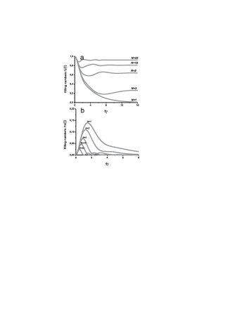
Figure 1: Filling numbers time evolution a). in the QD with the initial charge and b). in the central QD for the different number of QDs. Parameter $T/\gamma=0.6$ is the same for all the figures.

Filling numbers time evolution within the dot with initial charge $n_{j}(t)$ and within the central QD $n_{a}(t)$ in the absence of on-site Coulomb repulsion is presented on the Fig.1. The non-resonant tunneling between the dots is considered ($(\varepsilon-\varepsilon_{0})/\gamma=-1$).

It is clearly evident that filling numbers relaxation changes significantly with the increasing of QDs number $N$. When initial charge is localized in one of the $N$ QDs it remains confined in the initial dot even in the presence of relaxation processes from the central dot to the reservoir for the large number of dots. When one considers two surrounding dots only twenty percent of charge continue being localized in the initial QD (Fig.1a). But for ten interacting QDs more then eighty percent of charge is confined in the initial dot (Fig.1a). This effect can be called ”charge trapping” and the proposed system of coupled QDs can be considered as a ”charge trap”. QDs number $N$ increasing also leads to the decreasing of charge amplitude in the central QD $n_{a}(t)$ for a fixed value of ratio $T/\gamma$ due to the effective growth of tunneling coupling (Fig.1b).

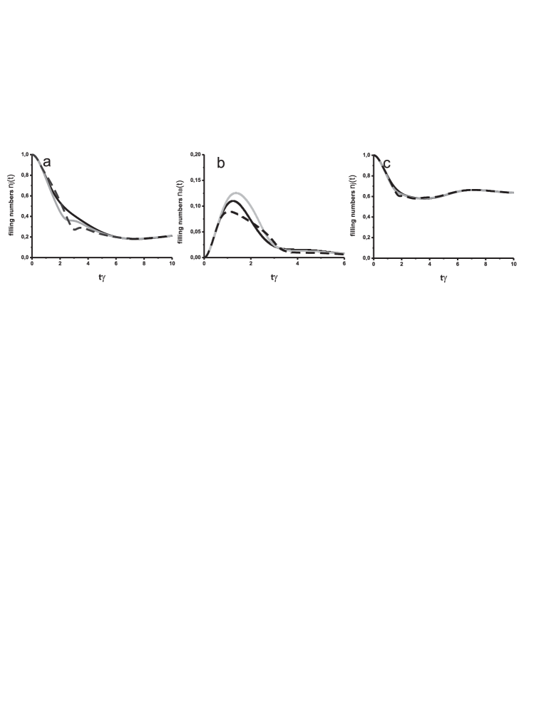
Figure 2: Filling numbers time evolution a),c). in the QD with initial charge and b). in the central QD for the different number of QDs a),b). $N=2$ and c). $N=5$. Coulomb interaction is taken into account in the central QD: $U/\gamma=0$-black line, $U/\gamma=10$-grey line and $U/\gamma=30$-black-dashed line. Parameter $T/\gamma=0.6$ is the same for all the figures.

Typical calculation results, in the case when on-site Coulomb repulsion is considered only in the central QD where localized charge is absent at the initial time moment, are demonstrated on the Fig.2. ”Charge trapping” effect is clearly evident with the increasing of QDs number even in the presence of Coulomb interaction between localized electrons (Fig.2).

For two QDs interacting with the central one Coulomb correlations strongly influence on the filling numbers relaxation (Fig.2a). A critical value of on-site Coulomb repulsion exists for a given set of system parameters which corresponds to the full compensation of the initial negative detuning Arseyev_2 . For the smaller values of Coulomb interaction, correlations lead to the increasing of relaxation rate in the QD with the initial charge (Fig.2a grey line) in comparison with the case when Coulomb interaction is absent (Fig.2a black line), due to the decreasing of the initial detuning value. For the values of on-site Coulomb repulsion larger than the critical one, positive detuning occurs and filling numbers relaxation rate decreases as a result of positive detuning value increasing (Fig.2a black-dashed line).

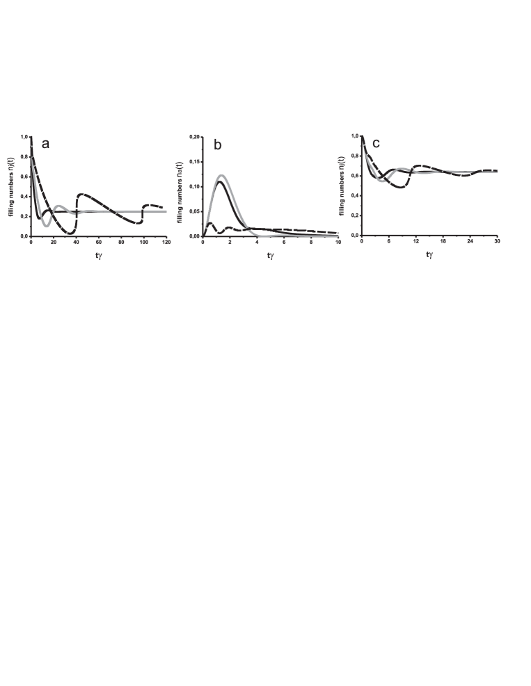
Figure 3: Filling numbers time evolution a),c). in the QD with initial charge and b). in the central QD for the different number of QDs a),b). $N=2$ and c). $N=5$. Coulomb interaction is taken into account in the QD with initially localized charge: $U=0$-black line, $U/\gamma=2$-grey line and $U/\gamma=7$-black-dashed line. Parameter $T/\gamma=0.6$ is the same for all the figures.

With the increasing of QDs number all the effects mentioned above are still valid, but they are less pronounced (Fig.2c). So the role of Coulomb correlations is suppressed for the large number of QDs due to the decreasing of electrons occupation in the central dot.

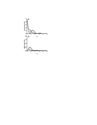
Figure 4: Filling numbers time evolution a),c). in the central QD with initial charge and b),d). in one of the $N$ surrounding QDs for a),b). $N=2$ and c),d). $N=10$. Coulomb interaction is taken into account in the central QD: $U/\gamma=0$-black line, $U/\gamma=4$-grey line and $U/\gamma=8$-black-dashed line. Parameter $T/\gamma=0.6$ is the same for all the figures.

Let us now analyze the situation when Coulomb interaction between localized electrons is taken into account within all the $N$ QDs which interact with the central one. Calculation results are presented on the Fig.3a and demonstrate ”charge trapping” effect with the increasing of the QDs number. In the case of two QDs interacting with the central one Coulomb correlations reveal significantly stronger influence on the filling numbers relaxation processes in comparison with the geometry when five dots are considered (Fig.3c).

Again two typical relaxation regimes were revealed. The first one corresponds to the decreasing of initial negative detuning value. In this regime Coulomb correlations lead to the increasing of relaxation rate in the QD with initial charge in comparison with the case when Coulomb interaction is absent (Fig.3a grey and black lines correspondingly). The second one deals with the Coulomb energy values large enough to compensate negative detuning and to form the positive one. In this regime filling numbers relaxation rate decreases as a result of positive detuning value increasing caused by the Coulomb interaction (Fig.3a grey and black-dashed lines correspondingly).

QDs number increasing also results in the increasing of filling numbers oscillations frequency. Filling numbers oscillations frequency for the small Coulomb values decreases corresponding to the detuning decreasing and increases as a result of positive detuning formation (Fig.3a,c). We found the growth of charge amplitude in the central QD with the increasing of the dots number when the negative detuning value decreases and amplitude decreasing when positive detuning value increases (Fig.3b).

When initial charge is localized in the central QD which is connected not only to the surrounding QDs but also to the continuous spectrum states ”charge trapping” effect doesn’t exist at all (Fig.4).

We now introduce the possible QDs geometry which allows to perform an experimental observations of charge trapping effects within the single dot. The most simple configuration is: $N$ similar lateral QDs interacting only with the single vertically aligned dot. Single vertical dot is also connected to the continuous spectrum states. But this geometry reveals a problem of initial charge localization. Initial charge can be localized in the single QD in the most simple way by means of the gate voltage. So it is convenient to have a system with $N-1$ lateral dots and single vertical dot with the localized charge. These $N$ dots interact only with the single central vertically aligned QD also connected to the continuous spectrum states.

To conclude, we have analyzed time evolution of the electron filling numbers in the system of $N$ interacting QDs both in the absence and in the presence of Coulomb interaction between localized electrons within the dots. It was found that Coulomb interaction modifies the relaxation rates and the character of localized charge time evolution. It was shown that several time ranges with considerably different relaxation rates arise in the system of coupled QDs. We demonstrated and carefully analyzed the presence of strong charge trapping effects in the proposed systems. It was found that interacting dots can form an effective high quality charge trap. We also revealed the Coulomb correlations suppression with the increasing of QDs number.

The QDs geometry which allows to perform an experimental observations of charge trapping effects was suggested.

This work was partly supported by the RFBR grants.

References

- (1) W. G. van derWiel, S. De Franceschi, J. M. Elzerman et.al., Rev. Mod. Phys., 75, 1 (2002).
- (2) R. M. Potok, I. G. Rau, H. Shtrikman et.al., Nature, 446, 167 (2007).
- (3) T. Hayashi, T. Fujisawa, H. D. Cheong et.al., Phys. Rev. Lett., 91, 226804 (2003).
- (4) C.A. Stafford, S. Das Sarma, Phys. Rev. Lett., 72, 3590 (1994).
- (5) K.A. Matveev, L.I. Glazman, H.U. Baranger, Phys. Rev. B, 54, 5637 (1996).
- (6) D. Boese, W. Hofstetter, H. Schoeller, Phys. Rev. B, 66, 125315 (2002).
- (7) K. Kikoin, Y. Avishai, Phys. Rev. B, 65, 115329 (2002).
- (8) P.A. Orellana, G.A. Lara, E.V. Anda, Phys. Rev. B, 65, 155317 (2002).
- (9) P.I. Arseyev, N.S. Maslova, V.N. Mantsevich, Solid State Comm., 152, 1545 (2012).
- (10) P.I. Arseyev, N.S. Maslova, V.N. Mantsevich, European Physical Journal B, 85(7), 249 (2012).
- (11) C.A. Stafford, N. Wingreen, Phys. Rev. Lett., 76, 1916 (1996).
- (12) B.L. Hazelzet, M.R. Wegewijs, T. H. Stoof, Phys. Rev. B, 63, 165313 (2001).
- (13) E. Cota, R. Aguadado, G. Platero, Phys. Rev. Lett., 94, 107202 (2005).
- (14) L.D. Contreras-Pulido, J. Splettstoesser, M. Governale et.al., Phys. Rev. B, 85, 075301 (2012).
- (15) Florian Elste, David R. Reichman, and Andrew J. Millis, Phys. Rev. B, 81, 205413 (2010).
- (16) D. M. Kennes, S. G. Jakobs, C. Karrasch et.al., Phys. Rev. B, 85, 085113 (2012).
- (17) M. A. Kastner, Rev. Mod. Phys., 64, 849 (1992).
- (18) C. W. J. Beenakker, Phys. Rev. B, 44, 1646 (1991).
- (19) Y. Alhassid, Rev. Mod. Phys., 72, 895 (2000).
- (20) A.N. Vamivakas, C.-Y. Lu, C. Matthiesen et.al., Nature Letters, 467, 297 (2010).
- (21) E.A. Stinaff, M. Scheibner, A.S. Bracker et.al., Science, 311, 636 (2006).
- (22) M. A. Kastner, Phys. Today, 46(1), 24 (1993).
- (23) R.C. Ashoori, Nature, 379, 413 (1996).
- (24) I. Chan, P. Fallahi, A. Vidan et.al., Nanotechnology, 15, 609 (2004).
- (25) M. Kuno, D.P. Fromm, H.F. Hamann et.al., J. Chem. Phys., 112, 3117 (2000).
- (26) M. Kuno, D.P. Fromm, H.F. Hamann et.al., J. Chem. Phys., 115, 1028 (2001).
- (27) M.R. Hummon, A.J. Stollenwerk, V. Narayanamurti, Phys. Rev. B, 81, 115439 (2010).
- (28) J.A. Brum, P. Hawrylak, Superlattices Microstruct., 22, 431 (1997).
- (29) M. Pioro-Ladriere, M.R. Abolfath, P. Zawadzki et.al., Phys. Rev. B, 72, 125307 (2005).
- (30) Bhalchandra. S. Pujari, Kavita Joshi, D.G. Kanhere et.al., Phys. Rev. B, 78, 125414 (2008).
- (31) L.V.Keldysh, Sov. Phys JETP, 20, 1018 (1964).
- (32) K. Kikoin, Y. Avishai, Phys. Rev. Lett., 86, 2090 (2001).
- (33) P. Coleman, Phys. Rev. B, 29, 3035 (1984).
- (34) S.M. Reimann, M. Manninen, Rev. Mod. Phys., 74, 1283 (2002).
- (35) W.M.C. Foulkes, L. Mitas, R.J. Needs et.al., Rev. Mod. Phys., 73, 33 (2001).
- (36) F.W. Cummings Phys. Rev. A, 33, 1683 (1986).