Towards Ultrahigh Dimensional Feature Selection
for Big Data

Abstract

In this paper, we present a new adaptive feature scaling scheme for ultrahigh-dimensional feature selection on Big Data. To solve this problem effectively, we first reformulate it as a convex semi-infinite programming (SIP) problem and then propose an efficient feature generating paradigm. In contrast with traditional gradient-based approaches that conduct optimization on all input features, the proposed method iteratively activates a group of features and solves a sequence of multiple kernel learning (MKL) subproblems of much reduced scale. To further speed up the training, we propose to solve the MKL subproblems in their primal forms through a modified accelerated proximal gradient approach. Due to such an optimization scheme, some efficient cache techniques are also developed. The feature generating paradigm can guarantee that the solution converges globally under mild conditions and achieve lower feature selection bias. Moreover, the proposed method can tackle two challenging tasks in feature selection: 1) group-based feature selection with complex structures and 2) nonlinear feature selection with explicit feature mappings. Comprehensive experiments on a wide range of synthetic and real-world datasets containing tens of million data points with $O(10^{14})$ features demonstrate the competitive performance of the proposed method over state-of-the-art feature selection methods in terms of generalization performance and training efficiency.

Keywords: Big data, Ultrahigh dimensionality, feature selection, nonlinear feature selection, multiple kernel learning, feature generation

1 Introduction

With the rapid development of the Internet, Big Data, with large volumes and ultrahigh dimensionality, has emerged in various machine learning applications, such as text mining and information retrieval (Deng et al., 2011; Li et al., 2011, 2012). For instance, a collaborative email-spam filtering task with 16 trillion ($10^{13}$) unique features has been studied in (Weinberger et al., 2009). Ultrahigh-dimensional data also widely appears in many nonlinear machine learning tasks. To tackle the intrinsic nonlinearity of Big Data, researchers have proposed to achieve fast training and prediction through linear techniques using explicit feature mappings (Chang et al., 2010; Maji and Berg, 2009). However, most of the explicit feature mappings dramatically expand the dimensionality of the data. For instance, the commonly used $2$-degree polynomial kernel feature mapping has a dimensionality of $O(m^{2})$ where $m$ denotes the number of input features (Chang et al., 2010). Even with a modest $m$, the dimensionality of the induced feature space is very large. Other typical feature mappings include the spectrum-based feature mapping for string kernels (Sonnenburg et al., 2007; Sculley et al., 2006), the histogram intersection kernel feature expansion (Wu, 2012), etc.

The ultrahigh dimensionality not only incurs the large memory requirements and high computational costs for training but also deteriorates the generalizability due to the “curse of dimensionality” (Duda et al., 2000.; Guyon and Elisseeff, 2003; Zhang and Lee, 2006; Dasgupta et al., 2007; Blum et al., 2007). Fortunately, in many datasets with ultrahigh dimensions, most of the features are irrelevant to the output. Accordingly, selecting the most informative features and dropping irrelevant features can vastly improve generalization performance (Ng, 1998). Moreover, for ultrahigh-dimensional problems, a sparse classifier is useful for faster predictions. Last, in many applications such as bioinformatics (Guyon and Elisseeff, 2003), a small number of features are expected to interpret the results for further biological analysis.

In recent decades, numerous feature selection methods have been proposed for classification tasks (Guyon et al., 2002; Chapelle and Keerthi, 2008). In general, existing feature methods can be classified into two categories: filter methods and wrapper methods (Kohavi and John, 1997; Ng, 1998; Guyon et al., 2002). Filter methods, such as the signal-to-noise ratio method (Golub et al., 1999) and spectral feature filtering (Zhao and Liu, 2007), have the advantage of low computational requirements but cannot identify the optimal feature subset for the predictive model of interest. In contrast, wrapper methods, which select the discriminative features by incorporating inductive learning rules, can achieve better performance than filter methods (Xu et al., 2009a; Guyon and Elisseeff, 2003), but incur a much higher computational cost. How to scale these wrapper methods to Big Data is a very challenging issue and is also the major focus of this paper.

As a typical wrapper method, the SVM-based recursive feature elimination (SVM-RFE) has shown good performance on a gene selection task in Microarray data analysis (Guyon et al., 2002). Specifically, using a recursive feature elimination scheme, SVM-RFE obtains nested subsets of features based on the weights of the classifier. Unfortunately, the nested feature selection strategy is “monotonic” and suboptimal in identifying the most informative feature subset (Xu et al., 2009a; Tan et al., 2010). To address this drawback, non-monotonic feature selection methods have gained much attention (Xu et al., 2009a; Chan et al., 2007). Basically, the non-monotonic feature selection requires the convexity of the objective such that a global solution exists. To this end, Chan et al. (2007) proposed two convex relaxations to the $\ell_{0}$-norm sparse SVM, QSSVM and SDP-SSVM, which are solved by convex quadratically constrained quadratic programming (QCQP) and semidefinite programming (SDP), respectively. The resultant models are convex, and thus they belong to the non-monotonic feature selection methods. However, these two models are too expensive to solve, especially for high dimensional problems. In addition, Xu et al.  proposed another non-monotonic feature selection method, namely NMMKL (Xu et al., 2009a). Since it involves a QCQP problem with many quadratic constraints, it is still computationally unfeasible for high-dimensional problems.

Focusing on the logistic loss, recently, some researchers have proposed selecting features using greedy strategies (Tewari et al., 2011; Lozano et al., 2011), which iteratively include one feature into a feature subset. For example, a group orthogonal matching pursuit (GOMP) is proposed in (Lozano et al., 2011). A more general greedy scheme is presented in (Tewari et al., 2011). Although promising performance has been observed, these greedy methods have some drawbacks. First, since only one feature is involved in each iteration, these methods are very expensive when there are a large number of features to be selected. More critically, due to the absence of an appropriate regularizer in the objective function, overfitting may occur, which will seriously deteriorate the generalization performance (Lozano et al., 2011; Tewari et al., 2011).

To avoid overfitting, one can add a regularizer to the loss function given a set of labeled patterns $\{{\bf x}_{i},y_{i}\}_{i=1}^{n}$ where ${\bf x}_{i}\in{\mathbb{R}}^{m}$ is an instance of $m$ dimensions and $y_{i}\in\{\pm 1\}$ is the output label. To select the most important features, we can learn a sparse decision function $d({\bf x})={\bf w}^{\prime}{\bf x}$ by solving the following:

$$\min_{\bf w}~{}~{}\|{\bf w}\|_{0}+C\sum\limits_{i=1}^{n}l(-y_{i}{\bf w}^{\prime}{\bf x}_{i}),$$ (1)

where ${\bf w}\in{\mathbb{R}}^{m}$ is the weight vector, $\|{\bf w}\|_{0}$ denotes the $\ell_{0}$-norm that counts the number of nonzeros in ${\bf w}$, $l(\cdot)$ is a convex loss function, and $C>0$ is a regularization parameter. Unfortunately, solving this problem is NP-hard due to the $\ell_{0}$-norm regularizer. Instead, many researchers resort to learning a sparse decision rule through an $\ell_{1}$-convex relaxation as follows (Bradley and Mangasarian, 1998; Zhu et al., 2003; Fung and Mangasarian, 2004):

$$\min_{\bf w}~{}~{}\|{\bf w}\|_{1}+C\sum\limits_{i=1}^{n}l(-y_{i}{\bf w}^{\prime}{\bf x}_{i}),$$ (2)

where $\|{\bf w}\|_{1}=\sum_{j=1}^{m}|w_{j}|$ is the $\ell_{1}$-norm on ${\bf w}$. The $\ell_{1}$-regularized problem can be efficiently solved because of its convexity. Recently, many optimization methods have been proposed to solve this including Newton methods (Fung and Mangasarian, 2004), proximal gradient methods (Yuan et al., 2011), coordinate descent methods (Yuan et al., 2010, 2011), etc. Interested readers can find more details of these methods in (Yuan et al., 2010, 2011) and references therein. Moreover, recently, much attention has been paid to online learning methods and stochastic gradient descent (SGD) methods for dealing with Big Data challenges (Xiao, 2009; Duchi and Singer, 2009; Langford et al., 2009; Shalev-Shwartz and Zhang, 2013).

However, there are several deficiencies regarding the $\ell_{1}$-norm regularized model and existing $\ell_{1}$-norm methods. First, since the $\ell_{1}$-norm regularization shrinks the regressors, feature selection bias will inevitably exist in $\ell_{1}$-norm methods (Zhang and Huang, 2008; Zhang, 2010b; Lin et al., 2010; Zhang, 2010a). Let $L({\bf w})=\sum_{i=1}^{n}l(-y_{i}{\bf w}^{\prime}{\bf x}_{i})$ be the empirical loss on the training data. Then, ${\bf w}^{*}$ is an optimal solution to (2) if and only if it satisfies the following optimality conditions (Yuan et al., 2010):

$$\left\{\begin{array}[]{ll}\nabla_{j}L({\bf w}^{*})=-{1}/{C}&\text{if}~{}~{}w_{j}^{*}>0,\\ \nabla_{j}L({\bf w}^{*})={1}/{C}&\text{if}~{}~{}w_{j}^{*}<0,\\ -{1}/{C}\leq\nabla_{j}L({\bf w}^{*})\leq{1}/{C}&\text{if}~{}~{}w_{j}^{*}=0.\\ \end{array}\right.$$ (3)

According to the above conditions, one can achieve different levels of sparsity by changing the regularization parameter $C$. Specifically, with a small $C$, minimizing $\|{\bf w}\|_{1}$ in (2) would favor selecting only a few features. However, the sparser the solution, the larger the predictive risk (or empirical loss) (Lin et al., 2010). In an extreme case where C is chosen to be very small (close to zero), none of the features will be selected according to the condition (3), which leads to a poor prediction model. To avoid this problem, we can learn an accurate prediction model using a larger $C$ (to reduce the empirical loss), which, however, will include more features according to (3). In other words, sparsity and unbiased solutions cannot be achieved simultaneously in (2) by changing the tradeoff parameter $C$. Following (Figueiredo et al., 2007; Zhang, 2010b), one remedy is to perform de-biasing with the detected features by retraining, which is equivalent to setting $C$ to $\infty$. However, such de-biasing methods that involve many times of retraining are not efficient. Moreover, when tackling Big Data with ultrahigh dimensions, the $\ell_{1}$-regularization will be inefficient or unfeasible. For example, when the dimensionality is approximately $10^{12}$, one needs approximately 1 TB of memory to store the weight vector ${\bf w}$, which is intractable for existing $\ell_{1}$-methods including online learning methods and SGD methods (Langford et al., 2009; Shalev-Shwartz and Zhang, 2013). Last, due to the scale variation of ${\bf w}$, it is also nontrivial to control the number of features while regulating the decision function.

In (Tan et al., 2010), the conference version of this paper, an $\ell_{0}$-norm sparse SVM model is introduced. Its nice optimization scheme has brought significant benefits to several applications, namely image retrieval (Rastegari et al., 2011), multi-label prediction (Gu et al., 2011a), feature selection for multivariate performance measures (Mao and Tsang, 2013), feature selection for logistic regression (Tan et al., 2013), and graph-based feature selection (Gu et al., 2011b). However, several issues remain to be solved. First, the tightness of the convex relation remains unclear. Second, the adopted optimization strategy is incapable of dealing with very large-scale and ultrahigh-dimensional problems. Third, the presented feature selection strategy is limited to linear feature selections. However, in many applications, one needs to tackle features with complex structures.

Regarding the above issues, in this paper, we propose an adaptive feature scaling (AFS) for feature selection by introducing a continuous feature scaling vector ${\bf d}\in[0,1]^{m}$. To enforce sparsity, we impose an explicit $\ell_{1}$-constraint $||{\bf d}||_{1}\leq B$, where the scalar $B$ represents the least number of features to be selected. The solution to the resulting optimization problem is nontrivial due to the additional constraint. Fortunately, by transforming it into a convex semi-infinite programming (SIP) problem, an efficient optimization scheme can be developed. In summary, this paper makes the following extensions and improvements.

• A Feature Generating Machine (FGM) is proposed to efficiently solve the SIP problem. Instead of performing the optimization on all input features, this method iteratively infers the most informative features and then solves a reduced subproblem using multiple kernel learning (MKL) methods in which each base kernel is defined on a set of the most informative features.

• A major advantage of this scheme is that the feature selection bias in the $\ell_{1}$-regularized methods can be alleviated by separately controlling the complexity and sparsity of the decision function. Particularly, the proposed optimization scheme mimics the retraining strategy to reduce the feature selection bias with little effort.

• To speed up the training on Big Data, we propose to solve the primal form of the MKL subproblem through a modified accelerated proximal gradient method. Accordingly, the large memory requirement and heavy computational costs can be significantly reduced. The convergence rate of the modified APG is provided. Several cache techniques are proposed to further enhance the efficiency.

• The feature generating paradigm is also extended to group feature selection with complex structures and nonlinear feature selection with explicit feature mappings.

The remainder of this paper is organized as follows. In Section 2, we start by presenting the adaptive feature scaling (AFS) for the linear feature selection task, group feature selection task and the corresponding convex reformulations. After that, in Section 3, we present the feature generating machine (FGM) to solve the resulting optimization problems, which include two core steps. These are the worst-case analysis step and the subproblem optimization step. In Section 4, we illustrate the details of the worst-case analysis for a number of learning tasks including feature selection with complex group structures and nonlinear feature selection with explicit feature mappings. We detail the subproblem optimization in Section 5. In Section 6, we extend FGM to do nonlinear feature selection with kernels. The connections to related studies are discussed in Section 7. We conduct comprehensive experiments in Section 8 and conclude this work in Section 9.

2 Feature Selection Through Adaptive Feature Scaling

Throughout this paper, we denote the transpose of a vector/matrix by the superscript ^′, a vector with all entries equal to one as $\textbf{1}\in{\mathbb{R}}^{n}$ and the zero vector as $\textbf{0}\in{\mathbb{R}}^{n}$. In addition, we denote a dataset by ${{\bf X}}=[{{{\bf x}}_{1}},...,{{{\bf x}}_{n}}]^{\prime}=[{{\bf f}}^{1},...,{{\bf f}}^{m}]$, where ${{\bf x}}_{i}\in{\mathbb{R}}^{m}$ represents the $i$th instance and ${\bf f}^{j}\in{\mathbb{R}}^{n}$ denotes the $j$th feature vector. We use $|\mathcal{G}|$ to denote cardinality of an index set $\mathcal{G}$ and $|v|$ to denote the absolute value of a real number $v$. For simplicity, we denote ${\bf v}\succeq\alpha$ if $v_{i}\geq\alpha,\forall i$ and ${\bf v}\preceq\alpha$ if $v_{i}\leq\alpha,\forall i$. We also denote $\|{\bf v}\|_{p}$ as the $\ell_{p}$-norm of a vector and $\|{\bf v}\|$ as the $\ell_{2}$-norm of a vector. Given a vector ${{\bf v}}=[{\bf v}_{1}^{\prime},...,{\bf v}_{p}^{\prime}]^{\prime}$ where ${\bf v}_{i}$ denotes a sub-vector of ${\bf v}$, we denote $\|{\bf v}\|_{2,1}=\sum_{i=1}^{p}\|{\bf v}_{i}\|_{2}$ as the mixed $\ell_{1}$/$\ell_{2}$ norm (Bach et al., 2011) and $\|{\bf v}\|_{2,1}^{2}=(\sum_{i=1}^{p}\|{\bf v}_{i}\|_{2})^{2}$. Accordingly, we call $\|{\bf v}\|_{2,1}^{2}$ an $\ell_{2,1}^{2}$ regularizer. Following (Rakotomamonjy et al., 2008), we define $\frac{x_{i}}{0}=0$ if $x_{i}=0$ and $\infty$ otherwise. Last, $\bf A\odot\bf B$ represents the element-wise product between two matrices $\bf A$ and $\bf B$.

2.1 A New AFS Scheme for Feature Selection

In SVM, we learn a linear decision function $d({\bf x})={\bf w}^{\prime}{\bf x}-b$ by solving the following problem:

$$\min_{\bf w}~{}~{}\frac{1}{2}\|{\bf w}\|^{2}+C\sum\limits_{i=1}^{n}l(-y_{i}({\bf w}^{\prime}{\bf x}_{i}-b)),$$ (4)

where ${\bf w}=[w_{1},\ldots,w_{m}]^{\prime}\in{\mathbb{R}}^{m}$ denotes the weight of the decision hyperplane, $b$ denotes the shift from the origin, $C>0$ represents the regularization parameter and $l(\cdot)$ denotes a convex loss function. In this paper, we concentrate on the squared hinge loss

$$l(-y_{i}({\bf w}^{\prime}{\bf x}_{i}-b))=\frac{1}{2}\max(1-y_{i}({\bf w}^{\prime}{\bf x}_{i}-b),0)^{2}$$

and the logistic loss

$$l(-y_{i}({\bf w}^{\prime}{\bf x}_{i}-b))=\log(1+\exp(-y_{i}({\bf w}^{\prime}{\bf x}_{i}-b))).$$

The $\ell_{2}$-regularizer $||{\bf w}||^{2}$, which is used to avoid the overfitting problem (Hsieh et al., 2008), cannot induce a sparse solution. To address this issue, we introduce a feature scaling vector ${\bf d}\in[0,1]^{m}$ to scale the importance of features. Given an instance ${\bf x}_{i}$, we impose $\sqrt{{\bf d}}=[\sqrt{d_{1}},\ldots,\sqrt{d_{m}}]^{\prime}$ on its features (Vishwanathan et al., 2010) resulting in the following rescaled instance:

$$\widehat{{\bf x}}_{i}=({\bf x}_{i}\odot\sqrt{\bf d}).$$ (5)

With this scaling scheme, the $j$th feature is selected if and only if $d_{j}>0$. Similar feature scaling schemes can be found in (Weston et al., 2000; Chapelle et al., 2002; Grandvalet and Canu, 2002; Rakotomamonjy, 2003; Varma and Babu, 2009; Vishwanathan et al., 2010). However, unlike these scaling schemes, ${\bf d}$ in (5) is bounded in $[0,~{}1]^{m}$.

In many real-world applications, one may intend to select a desired number of features with acceptable generalization performance. For example, in Microarray data analysis, due to expensive biodiagnosis and limited resources, biologists prefer to select less than 100 genes from hundreds of thousands of genes (Guyon et al., 2002; Golub et al., 1999). Motivated by such prior knowledge, to select features, we explicitly constrain the $\ell_{1}$-norm of ${\bf d}$ by the following:

$$\sum\limits_{j=1}^{m}d_{j}=||{\bf d}||_{1}\leq B,~{}d_{j}\in[0,1],~{}j=1,\cdots,m,$$ (6)

where the integer $B$ represents the least number of features to be selected. Let $\mathcal{D}=\big{\{}{\bf d}\in\mathbb{R}^{m}\big{|}\sum_{j=1}^{m}d_{j}\leq B,~{}d_{j}\in[0,1],~{}j=1,\cdots,m\big{\}}$ be the domain of ${\bf d}$. Note that the compact domain $\mathcal{D}$ contains an infinite number of elements. Herein, for simplicity, we concentrate on the squared hinge loss. Accordingly, the proposed AFS can be formulated as follows:

$$\min\limits_{{\bf d}\in{\mathcal{D}}}\min\limits_{{\bf{w}},\mbox{{\boldmath$\xi$}},b} \frac{1}{2}\|{\bf{w}}\|_{2}^{2}+{\frac{C}{2}\sum\limits_{i=1}^{n}\xi^{2}_{i}}$$ (7)

s.t. $${y_{i}\left({\bf{w}}^{\prime}({\bf x}_{i}\odot\sqrt{\bf d})-b\right)\geq 1-\xi_{i}},\;\;\;\;i=1,\cdots,n,$$

where $C$ is the regularization parameter that trades off between the model complexity and the fitness of the decision function, and $b/\|{\bf{w}}\|$ determines the offset of the hyperplane from the origin along the normal vector ${\bf w}$. This problem is a non-convex optimization problem. For a fixed ${\bf d}$, it indexes a set of features. Accordingly, the inner minimization problem with respect to ${\bf{w}}$ and $\xi$ is a standard SVM problem as follows:

$$\min\limits_{{\bf{w}},\mbox{{\boldmath$\xi$}},b} \frac{1}{2}\|{\bf{w}}\|_{2}^{2}+{\frac{C}{2}\sum\limits_{i=1}^{n}\xi^{2}_{i}}$$ (8)

s.t. $${y_{i}\left({\bf{w}}^{\prime}({\bf x}_{i}\odot\sqrt{\bf d})-b\right)\geq 1-\xi_{i}},\;\;\;\;i=1,\cdots,n,$$

which can be solved in its dual form. By introducing the Lagrangian multiplier $\alpha_{i}\geq 0$ to each constraint ${y_{i}\left({\bf{w}}^{\prime}({\bf x}_{i}\odot\sqrt{\bf d})-b\right)\geq 1-\xi_{i}}$, the Lagrangian function is as follows:

$${\mathcal{L}}({\bf w},\mbox{{\boldmath$\xi$}},b,\mbox{{\boldmath$\alpha$}})=\frac{1}{2}\|{\bf{w}}\|_{2}^{2}+\frac{C}{2}\sum\limits_{i=1}^{n}\xi^{2}_{i}-\sum_{i=1}^{n}{\alpha_{i}}\left(y_{i}\left({\bf{w}}^{\prime}({\bf x}_{i}\odot\sqrt{\bf d})-b\right)-1+\xi_{i}\right).$$ (9)

By setting the derivatives of ${\mathcal{L}}({\bf w},\mbox{{\boldmath$\xi$}},b,\mbox{{\boldmath$\alpha$}})$ w.r.t. ${\bf w}$, $\xi$ and $b$ to ${\bf 0}$, we get the following:

$${\bf w}=\sum_{i=1}^{n}{\alpha_{i}}{y_{i}({\bf x}_{i}\odot\sqrt{\bf d})},\mbox{{\boldmath$\alpha$}}=C\mbox{{\boldmath$\xi$}},~{}\text{and}~{}\sum_{i=1}^{n}\alpha_{i}y_{i}=0.$$ (10)

Substituting these results into (9), we obtain the dual form of (8) as follows:

$$\max_{\mbox{{\boldmath$\alpha$}}\in\mathcal{A}}~{}~{}-\frac{1}{2}\bigg{\|}\sum_{i=1}^{n}\alpha_{i}y_{i}({\bf x}_{i}\odot\sqrt{\bf d})\bigg{\|}^{2}-\frac{1}{2C}\mbox{{\boldmath$\alpha$}}^{\prime}\mbox{{\boldmath$\alpha$}}+\mbox{{\boldmath$\alpha$}}^{\prime}{\bf 1},$$ (11)

where ${\cal A}=\{\mbox{{\boldmath$\alpha$}}|\sum_{i=1}^{n}\alpha_{i}y_{i}=0,\mbox{{\boldmath$\alpha$}}\succeq{\bf 0}\}$ is the domain of $\alpha$. For convenience, let ${\bf c}(\mbox{{\boldmath$\alpha$}})=\sum_{i=1}^{n}\alpha_{i}y_{i}{\bf x}_{i}\in{\mathbb{R}}^{m}$; then, we have $\bigg{\|}\sum_{i=1}^{n}\alpha_{i}y_{i}({\bf x}_{i}\odot\sqrt{\bf d})\bigg{\|}^{2}=\sum_{j=1}^{m}d_{j}[c_{j}(\mbox{{\boldmath$\alpha$}})]^{2}$ where $c_{j}(\mbox{{\boldmath$\alpha$}})$ denotes the $j$th coordinate of ${\bf c}(\mbox{{\boldmath$\alpha$}})$ and is a function of $\alpha$. For simplicity, let

$$f(\mbox{{\boldmath$\alpha$}},{\bf d})=\frac{1}{2}\sum_{j=1}^{m}d_{j}[c_{j}(\mbox{{\boldmath$\alpha$}})]^{2}+\frac{1}{2C}\mbox{{\boldmath$\alpha$}}^{\prime}\mbox{{\boldmath$\alpha$}}-\mbox{{\boldmath$\alpha$}}^{\prime}{\bf 1}.$$

Apparently, $f(\mbox{{\boldmath$\alpha$}},{\bf d})$ is linear in ${\bf d}$ and concave in $\alpha$, and both $\mathcal{A}$ and $\mathcal{D}$ are compact domains. Problem (7) can be equivalently reformulated as the following problem:

$$\min\limits_{{\bf d}\in\mathcal{D}}\max\limits_{\mbox{{\boldmath$\alpha$}}\in\mathcal{A}}~{}~{}-f(\mbox{{\boldmath$\alpha$}},{\bf d}),$$ (12)

However, this problem is still difficult to address. According to the minimax saddle-point theorem (Sion, 1958), we immediately have the following relation.

Theorem 1

Since both $\mathcal{A}$ and ${\mathcal{D}}$ are convex compact sets, according to the minimax saddle-point theorem (Sion, 1958) the following equality holds by interchanging the order of $\min_{{\bf d}\in{\mathcal{D}}}$ and $\max_{\mbox{{\boldmath$\alpha$}}\in\mathcal{A}}$ in (12):

$$\min\limits_{{\bf d}\in\mathcal{D}}\max\limits_{\mbox{{\boldmath$\alpha$}}\in\mathcal{A}}~{}~{}-f(\mbox{{\boldmath$\alpha$}},{\bf d})=\max\limits_{\mbox{{\boldmath$\alpha$}}\in\mathcal{A}}\min\limits_{{\bf d}\in\mathcal{D}}~{}~{}-f(\mbox{{\boldmath$\alpha$}},{\bf d}).$$ (13)

Based on the above equality, hereafter we address (12) by solving the following minimax problem instead:

$$\min\limits_{\mbox{{\boldmath$\alpha$}}\in\mathcal{A}}\max\limits_{{\bf d}\in\mathcal{D}}~{}~{}f(\mbox{{\boldmath$\alpha$}},{\bf d}).$$ (14)

2.2 AFS for Group Feature Selection

The AFS scheme for linear feature selection can be easily extended for group feature selection where the features are organized by a group structure $\mathcal{G}=\{\mathcal{G}_{1},...,\mathcal{G}_{p}\}$. Here, $p=|\mathcal{G}|$ denotes the number of groups and $\cup_{j=1}^{p}\mathcal{G}_{j}=\{1,...,m\}$, and $\mathcal{G}_{j}\subset\{1,...,m\},j=1,...,p$ denotes the index set of feature supports belonging to the $j$th group of features. In group feature selection, a feature in one group is selected if and only if this group is selected (Yuan and Lin, 2006; Meier et al., 2008). Let ${\bf w}_{\mathcal{G}_{j}}\in{\mathbb{R}}^{|\mathcal{G}_{j}|}$ and ${\bf x}_{\mathcal{G}_{j}}\in{\mathbb{R}}^{|\mathcal{G}_{j}|}$ be the components of ${\bf w}$ and ${\bf x}$ related to $\mathcal{G}_{j}$, respectively. The group feature selection is usually achieved by solving the following non-smooth group lasso problem (Yuan and Lin, 2006; Meier et al., 2008):

$$\min_{\bf w}~{}~{}\lambda\sum_{j=1}^{p}||{\bf w}_{\mathcal{G}_{j}}||_{2}+\sum\limits_{i=1}^{n}l(-y_{i}\sum_{j=1}^{p}{\bf w}_{\mathcal{G}_{j}}^{\prime}{\bf x}_{i}{{}_{\mathcal{G}_{j}}}),$$ (15)

where $\lambda$ denotes the trade-off parameter. To solve this problem, many efficient algorithms have been proposed, such as accelerated proximal gradient descent methods (Liu and Ye, 2010; Jenatton et al., 2011b; Bach et al., 2011), block coordinate descent methods (Qin et al., 2010; Jenatton et al., 2011b) and active set methods (Bach, 2009; Roth and Fischer, 2008). However, the same issues with the $\ell_{1}$-regularization, namely, the scalability issue for Big Data and feature selection bias, will occur when performing group feature selection via solving (15). Moreover, when dealing with groups with complex structures, the number of groups can be exponential in the number of features $m$. As a result, solving (15) could be very expensive.

To extend the AFS for linear feature selection to group feature selection, we introduce a group scaling vector $\widehat{\bf d}=[\widehat{d}_{1},\ldots,\widehat{d}_{p}]^{\prime}\in\widehat{\mathcal{D}}$ to scale the groups where $\widehat{\mathcal{D}}=\big{\{}\widehat{{\bf d}}\in\mathbb{R}^{p}\big{|}\sum_{j=1}^{p}\widehat{d}_{j}\leq B,\widehat{d}_{j}\in[0,1],~{}j=1,\cdots,p\big{\}}$. Without loss of generality, we first assume that there are no overlapping elements among groups, namely, $\mathcal{G}_{i}\cap\mathcal{G}_{j}=\emptyset,\forall i\neq j$. Accordingly, we have ${\bf w}=[{\bf w}_{\mathcal{G}_{1}}^{\prime},...,{\bf w}_{\mathcal{G}_{p}}^{\prime}]^{\prime}\in{\mathbb{R}}^{m}$. By taking the shift term $b$ into consideration, the decision function is expressed as follows:

$$q({\bf x})=\sum\limits_{j=1}^{p}{\sqrt{\widehat{d}_{j}}}{\bf w}_{\mathcal{G}_{j}}^{\prime}{\bf x}_{\mathcal{G}_{j}}-b,$$

Focusing on the squared hinge loss, the AFS-based group feature selection can be formulated as the following problem:

$$\min\limits_{\widehat{\bf d}\in\widehat{{\mathcal{D}}}}\min\limits_{{\bf{w}},\mbox{{\boldmath$\xi$}},b} \frac{1}{2}\|{\bf w}\|_{2}^{2}+\frac{C}{2}\sum\limits_{i=1}^{n}\xi^{2}_{i}$$ (16)

s.t. $$y_{i}\left(\sum\limits_{j=1}^{p}\sqrt{\widehat{d}_{j}}{\bf w}_{\mathcal{G}_{j}}^{\prime}{\bf x}_{i\mathcal{G}_{j}}-b\right)\geq 1-\xi_{i},\;\;\xi_{i}\geq 0,\;\;i=1,\cdots,n.$$

With similar deductions in Section 2.1, the above problem can be transformed into the following minimax problem:

$$\min\limits_{\widehat{\bf d}\in\widehat{{\mathcal{D}}}}\max\limits_{\mbox{{\boldmath$\alpha$}}\in\mathcal{A}}-\frac{1}{2}\sum\limits_{j=1}^{p}\widehat{d}_{j}\bigg{\|}\sum_{i=1}^{n}\alpha_{i}y_{i}{\bf x}_{i\mathcal{G}_{j}}\bigg{\|}^{2}-\frac{1}{2C}\mbox{{\boldmath$\alpha$}}^{\prime}\mbox{{\boldmath$\alpha$}}+\mbox{{\boldmath$\alpha$}}^{\prime}{\bf 1},$$ (17)

which will reduce to the linear case if $|\mathcal{G}_{j}|=1,\forall j=1,...,p$. Without loss of generality, we hereafter drop the hat from $\widehat{{\bf d}}$ and $\widehat{{\mathcal{D}}}$. Let

$${\bf c}_{\mathcal{G}_{j}}(\mbox{{\boldmath$\alpha$}})=\sum_{i=1}^{n}\alpha_{i}y_{i}{\bf x}_{i\mathcal{G}_{j}}$$

and define

$$f(\mbox{{\boldmath$\alpha$}},{\bf d})=\frac{1}{2}\sum_{j=1}^{p}d_{j}\left\|{\bf c}_{\mathcal{G}_{j}}(\mbox{{\boldmath$\alpha$}})\right\|^{2}+\frac{1}{2C}\mbox{{\boldmath$\alpha$}}^{\prime}\mbox{{\boldmath$\alpha$}}-\mbox{{\boldmath$\alpha$}}^{\prime}{\bf 1}.$$

Last, we arrive at the following unified minimax optimization problem:

$$\min\limits_{\mbox{{\boldmath$\alpha$}}\in\mathcal{A}}\max\limits_{{\bf d}\in\mathcal{D}}~{}~{}f(\mbox{{\boldmath$\alpha$}},{\bf d}),$$ (18)

where ${\mathcal{D}}=\big{\{}{{\bf d}}\in\mathbb{R}^{p}\big{|}\sum_{j=1}^{p}{d}_{j}\leq{B},~{}{d}_{j}\in[0,1],~{}j=1,\cdots,p\big{\}}$. When $|\mathcal{G}_{j}|=1,\forall j=1,...,p$, we have $p=m$, and problem (18) is reduced to problem (14).

2.3 Group Feature Selection with Complex Structures

The above AFS scheme can be extended to deal with group features with complex structures, such as groups with overlapping features or even more complex structures. When dealing with groups with overlapping features, a heuristic method is to explicitly augment ${{\bf X}}=[{\bf f}^{1},...,{\bf f}^{m}]$ to make the groups nonoverlapping by repeating the overlapping features. For example, suppose ${{\bf X}}=[{\bf f}^{1},{\bf f}^{2},{\bf f}^{3}]$ with groups $\mathcal{G}=\{\mathcal{G}_{1},\mathcal{G}_{2}\}$ where $\mathcal{G}_{1}=\{1,2\}$ and $\mathcal{G}_{2}=\{2,3\}$, and ${\bf f}^{2}$ is an overlapping feature. To avoid the overlapping element, we duplicate ${\bf f}^{2}$ and construct an augmented dataset such that ${{\bf X}}_{au}=[{\bf f}^{1},{\bf f}^{2},{\bf f}^{2},{\bf f}^{3}]$. After this, the group index sets become $\mathcal{G}_{1}=\{1,2\}$ and $\mathcal{G}_{2}=\{3,4\}$. This feature augmentation strategy can be extended to groups that have more complex structures, such as tree structures and graph structures (Bach, 2009). Here, we only study tree-structured groups, which are defined as follows.

Definition 1

Tree-structured set of groups (Jenatton et al., 2011b; Kim and Xing, 2010, 2012). A super set of groups $\mathcal{G}\triangleq\{\mathcal{G}_{h}\}_{\mathcal{G}_{h}\in\mathcal{G}}$ with $|\mathcal{G}|=p$ is said to be tree-structured in $\{1,...,m\}$, if $\cup\mathcal{G}_{h}=\{1,...,m\}$ and if for all $\mathcal{G}_{g},\mathcal{G}_{h}\in\mathcal{G}$, $(\mathcal{G}_{g}\cap\mathcal{G}_{h}\neq\varnothing)\Rightarrow(\mathcal{G}_{g}\subseteq\mathcal{G}_{h}~{}~{}\textrm{or}~{}~{}\mathcal{G}_{h}\subseteq\mathcal{G}_{g})$. For such a set of groups, there exists a (nonunique) total order relation $\preceq$ such that:

$$\mathcal{G}_{g}\preceq\mathcal{G}_{h}\Rightarrow\{\mathcal{G}_{g}\subseteq\mathcal{G}_{h}~{}\textrm{or}~{}\mathcal{G}_{g}\cap\mathcal{G}_{h}=\varnothing\}.$$

Similar to the overlapping case, we can augment the overlapping elements of all groups along the tree structures resulting in the augmented dataset ${{\bf X}}_{au}=[{{\bf X}}_{\mathcal{G}_{1}},...,{{\bf X}}_{\mathcal{G}_{p}}]$ where ${{\bf X}}_{\mathcal{G}_{i}}$ represents the data columns selected by ${\mathcal{G}_{i}}$ and $p$ denotes the number of all possible groups. However, this simple idea may bring large challenges for optimization; particularly when there are a large number of overlapping groups. For instance, in graph-based group structures, the number of groups $p$ can be exponential in $m$ (Bach, 2009). How to avoid this difficulty is one of the focuses of this paper.

3 Feature Generating Machine

Under the proposed AFS scheme, both the linear feature selection and the group feature selection can be cast as the minimax problem (18). By bringing in an additional variable $\theta\in{\mathbb{R}}$ and following (Pee and Royset, 2010), this problem can be further formulated as a semi-infinite programming (SIP) problem (Kelley, 1960; Pee and Royset, 2010):

$$\min\limits_{\mbox{{\boldmath$\alpha$}}\in\mathcal{A},\theta\in{\mathbb{R}}}\theta,~{}~{}\text{s.t.}~{}~{}~{}~{}\theta\geq f(\mbox{{\boldmath$\alpha$}},{\bf d}),~{}~{}\forall~{}{\bf d}\in\mathcal{D}.$$ (19)

In (19), each nonzero ${\bf d}\in\mathcal{D}$ defines a quadratic constraint (w.r.t. $\alpha$) $\theta\geq f(\mbox{{\boldmath$\alpha$}},{\bf d})$. Notice that there are an infinite number of ${\bf d}$’s in $\mathcal{D}$. Consequently, there are an infinite number of constraints involved in (19) making it difficult to solve.

3.1 Optimization Strategies by Feature Generation

Before solving (19), we first consider its optimality condition. Specifically, let $\mu_{h}\geq 0$ be the dual variable for each constraint $\theta\geq f(\mbox{{\boldmath$\alpha$}},{\bf d})$, then the Lagrangian function of (19) can be written as follows:

$$\mathcal{L}(\theta,\mbox{{\boldmath$\alpha$}},\textbf{$\mbox{{\boldmath$\mu$}}$})={\theta}-\sum_{{\bf d}_{h}\in\mathcal{D}}\mu_{h}\left(\theta-f(\mbox{{\boldmath$\alpha$}},{\bf d}_{h})\right).$$

By setting its derivative w.r.t. $\theta$ to zero, we have $\sum\mu_{h}=1$. Let $\mathcal{M}=\{\mbox{{\boldmath$\mu$}}|\sum\mu_{h}={1},\mu_{h}\geq 0,h=1,...,|\mathcal{D}|\}$ be the domain of $\mu$. We define the following:

$${f}_{\text{m}}(\mbox{{\boldmath$\alpha$}})=\max_{{\bf d}_{h}\in\mathcal{D}}f(\mbox{{\boldmath$\alpha$}},{\bf d}_{h}).$$

Then, the KKT conditions of (19) can be written as follows:

$$\sum\limits_{{\bf d}_{h}\in\mathcal{D}}\mu_{h}\nabla_{\mbox{{\boldmath$\alpha$}}}f(\mbox{{\boldmath$\alpha$}},{\bf d}_{h})={\bf 0},~{}~{}~{}~{}\text{and}~{}~{}~{}~{}\sum\limits_{{\bf d}_{h}\in\mathcal{D}}\mu_{h}=1.$$ (20)

$${\mu_{h}(f(\mbox{{\boldmath$\alpha$}},{\bf d}_{h})-f_{m}(\mbox{{\boldmath$\alpha$}}))=0,}~{}~{}~{}\mu_{h}\geq 0,~{}~{}h=1,...,|\mathcal{D}|.$$ (21)

Although there are many constraints in problem (3.1), most of them are nonactive at optimality if ${\bf X}$ only contains a small number of relevant features w.r.t. the output ${\bf y}$. Actually, according to the above conditions, we have $\mu_{h}=0$ if $f(\mbox{{\boldmath$\alpha$}},{\bf d}_{h})<{f}_{\text{m}}(\mbox{{\boldmath$\alpha$}})$, which induces sparsity among $\mu_{h}$’s. Motivated by this observation, we design an efficient optimization scheme that iteratively infers the active constraints and then solves a subproblem of reduced scale with the selected constraints. Accordingly, the computational burden brought by the infinite number of constraints can be avoided. The details of this algorithm are presented in Algorithm 1, which is also known as the cutting plane algorithm (Kelley, 1960; Mutapcic and Boyd, 2009).

Algorithm 1 Cutting Plane Algorithm for Solving (19) (Outer Iterations).

1:  Initialize $\mbox{{\boldmath$\alpha$}}^{0}=C\textbf{1}$ and $\mathcal{C}_{0}=\emptyset$. Set iteration index $t=1$.

2:   Feature Inference:   Do worst-case analysis to infer the most violated ${{\bf d}_{t}}$ based on $\mbox{{\boldmath$\alpha$}}^{t-1}$.   Set $\mathcal{C}_{t}=\mathcal{C}_{t-1}\bigcup\{{\bf d}_{t}\}$.

3:   subproblem Optimization:   Solve subproblem (22) obtaining the optimal solution $\mbox{{\boldmath$\alpha$}}^{t}$ and $\mu^{t}$.

4:  Let $t=t+1$. Repeat steps 2-3 until convergence.

Basically, Algorithm 1 involves two major steps: the feature inference step (also known as the worst-case analysis) and the subproblem optimization step. The whole procedure iterates until particular stopping conditions are achieved. Specifically, the worst-case analysis infers the most-violated ${\bf d}_{t}$ based on $\mbox{{\boldmath$\alpha$}}^{t-1}$ and adds it to the active constraint set $\mathcal{C}_{t}$. As will be shown later, in general, each active ${\bf d}_{t}\in\mathcal{C}_{t}$ contains $B$ new features. In this sense, we refer to Algorithm 1 as the Feature Generating Machine (FGM). Recall that, if there is no feature being selected, the empirical loss is $\mbox{{\boldmath$\xi$}}={\bf 1}$. Therefore, we initialize $\mbox{{\boldmath$\alpha$}}^{0}=C{\bf 1}$ according to the relation in (10). Once an active ${{\bf d}_{t}}$ is identified, we update $\mbox{{\boldmath$\alpha$}}^{t}$ by solving the following subproblem with the constraints defined in $\mathcal{C}_{t}$:

$$\min\limits_{\mbox{{\boldmath$\alpha$}}\in\mathcal{A},\theta\in{\mathbb{R}}}\theta,~{}~{}~{}~{}\text{s.t.}~{}~{}~{}~{}f(\mbox{{\boldmath$\alpha$}},{\bf d}_{h})-\theta\leq 0,~{}\forall~{}{\bf d}_{h}\in\mathcal{C}_{t}.$$ (22)

Since $|\mathcal{C}_{t}|=t$, problem (22) involves only $t$ constraints and thus is easier to address.

Last, after obtaining the optimal solution ${\bf d}^{*}$ to (22), the selected features (or the selected feature groups) are associated with the nonzero entries in ${\bf d}^{*}$.

3.2 Convergence Analysis

Before the introduction of the worst-case analysis and the solution to the subproblem, we first conduct a convergence analysis of Algorithm 1.

Without loss of generality, let $\mathcal{A}\times\mathcal{D}$ be the domain for problem (19). In the $(t+1)$th iteration, we find a new constraint ${\bf d}_{t+1}$ based on $\mbox{{\boldmath$\alpha$}}_{t}$ and add it to $\mathcal{C}_{t}$, i.e., $f(\mbox{{\boldmath$\alpha$}}_{t},{\bf d}_{t+1})=\max_{{\bf d}\in\mathcal{D}}f(\mbox{{\boldmath$\alpha$}}_{t},{\bf d})$. Apparently, we have $\mathcal{C}_{t}\subseteq\mathcal{C}_{t+1}$. For convenience, we define the following:

$$\begin{array}[]{l}\beta_{t}=\max\limits_{1\leq i\leq{t}}f(\mbox{{\boldmath$\alpha$}}_{t},{\bf d}_{i})=\min\limits_{\mbox{{\boldmath$\alpha$}}\in\mathcal{A}}\max\limits_{1\leq i\leq{t}}f(\mbox{{\boldmath$\alpha$}},{\bf d}_{i}).\end{array}$$ (24)

and

$$\varphi_{t}=\min\limits_{1\leq j\leq{t}}f(\mbox{{\boldmath$\alpha$}}_{j},{\bf d}_{j+1})=\min\limits_{1\leq j\leq{t}}(\max_{{\bf d}\in\mathcal{D}}f(\mbox{{\boldmath$\alpha$}}_{j},{\bf d})).~{}~{}$$ (25)

Following (Chen and Ye, 2008), we have the following lemma:

Lemma 1

Let $(\alpha^{*},\theta^{*})$ be a globally optimal solution of (19), and let $\{\theta_{t}\}$ and $\{\varphi_{t}\}$ be defined as above, then: $\theta_{t}\leq\theta^{*}\leq\varphi_{t}.$ With the number of iterations $t$ increasing, $\{\theta_{t}\}$ will monotonically increase and the sequence $\{\varphi_{t}\}$ will monotonically decrease.

Proof  According to the definition, we have $\theta_{t}=\beta_{t}$ Moreover, $\theta^{*}\!\!\!\!~{}=~{}\!\!\!\!\min_{\mbox{{\boldmath$\alpha$}}\in\mathcal{A}}\max_{{\bf d}\in\mathcal{D}}f(\mbox{{\boldmath$\alpha$}},{\bf d})$. For a fixed feasible $\alpha$, we have $\max_{{\bf d}\in\mathcal{C}_{t}}f(\mbox{{\boldmath$\alpha$}},{\bf d})\leq\max_{{\bf d}\in\mathcal{D}}f(\mbox{{\boldmath$\alpha$}},{\bf d})$, then

$$\min_{\mbox{{\boldmath$\alpha$}}\in\mathcal{A}}\max_{{\bf d}\in\mathcal{C}_{t}}f(\mbox{{\boldmath$\alpha$}},{\bf d})\leq\min_{\mbox{{\boldmath$\alpha$}}\in\mathcal{A}}\max_{{\bf d}\in\mathcal{D}}f(\mbox{{\boldmath$\alpha$}},{\bf d}),$$

that is, $\theta_{t}\leq\theta^{*}.$ On the other hand, for $\forall j=1,\cdots,k$, $f(\mbox{{\boldmath$\alpha$}}_{j},{\bf d}_{j+1})=\max_{{\bf d}\in\mathcal{D}}f(\mbox{{\boldmath$\alpha$}}_{j},{\bf d})$; thus, $(\mbox{{\boldmath$\alpha$}}_{j},f(\mbox{{\boldmath$\alpha$}}_{j},{\bf d}_{j+1}))$ is a feasible solution of (19). Then $\theta^{*}\leq f(\mbox{{\boldmath$\alpha$}}_{j},{\bf d}_{j+1})$ for $j=1,\cdots,{t}$, and hence we have the following:

$$\theta^{*}\leq\varphi_{t}=\min_{1\leq j\leq{t}}f(\mbox{{\boldmath$\alpha$}}_{j},{\bf d}_{j+1}).$$

With increasing iterations $t$, the subset $\mathcal{C}_{t}$ will monotonically increase. Thus, $\{\theta_{t}\}$ will monotonically increase, while $\{\varphi_{t}\}$ will monotonically decrease. QED  

The following conclusion shows that FGM converges to a global solution of (19).

Theorem 2

Assume that in Algorithm 1, the subproblem (22) and the worst-case analysis in step 2 can be solved. Let $\{(\mbox{{\boldmath$\alpha$}}_{t},\theta_{t})\}$ be the sequence generated by Algorithm 1. If Algorithm 1 terminates at iteration $(t+1)$, then $\{(\mbox{{\boldmath$\alpha$}}_{t},\theta_{t})\}$ is the global optimal solution of (19); otherwise, $(\mbox{{\boldmath$\alpha$}}_{t},\theta_{t})$ converges to a global optimal solution $(\mbox{{\boldmath$\alpha$}}^{*},\theta^{*})$ of (19).

Proof  We can measure the convergence of FGM by the gap difference between the series $\{\theta_{t}\}$ and $\{\varphi_{t}\}$. Assume in the $t$th iteration that there is no update of $\mathcal{C}_{t}$, i.e., ${\bf d}_{{t}+1}~{}=~{}\arg\max_{{\bf d}\in\mathcal{D}}f(\mbox{{\boldmath$\alpha$}}_{t},{\bf d})\in\mathcal{C}_{t},$ then $\mathcal{C}_{t}=\mathcal{C}_{{t}+1}$. In this case, $(\mbox{{\boldmath$\alpha$}}_{t},\theta_{t})$ is the globally optimal solution of (19). Actually, since $\mathcal{C}_{t}=\mathcal{C}_{{t}+1}$ in Algorithm 1, there will be no update of $\alpha$, i.e., $\mbox{{\boldmath$\alpha$}}_{{t}+1}=\mbox{{\boldmath$\alpha$}}_{t}$. Then, we have the following:

$$f(\mbox{{\boldmath$\alpha$}}_{t},{\bf d}_{{t}+1})=\max_{{\bf d}\in\mathcal{D}}f(\mbox{{\boldmath$\alpha$}}_{t},{\bf d})=\max_{{\bf d}\in\mathcal{C}_{t}}f(\mbox{{\boldmath$\alpha$}}_{t},{\bf d})=\max_{1\leq i\leq{t}}f(\mbox{{\boldmath$\alpha$}}_{t},{\bf d}_{i})=\theta_{t}$$

$$\varphi_{t}=\min\limits_{1\leq j\leq{t}}f(\mbox{{\boldmath$\alpha$}}_{j},{\bf d}_{j+1})\leq\theta_{t}.$$

According to Lemma 1, we have $\theta_{t}\leq\theta^{*}\leq\varphi_{t}$, and thus we have $\theta_{t}=\theta^{*}=\varphi_{t}$, and $(\mbox{{\boldmath$\alpha$}}_{t},\theta_{t})$ is the global optimum of (19).

Suppose that the algorithm does not terminate in finite steps. Let $\mathcal{X}=\mathcal{A}\times[\theta_{1},\theta^{*}]$, then a limit point $(\bar{\mbox{{\boldmath$\alpha$}}},\bar{\theta})$ exists for $(\mbox{{\boldmath$\alpha$}}_{t},\theta_{t})$ since $\mathcal{X}$ is compact. In addition, we also have $\bar{\theta}\leq\theta^{*}$. For each $t$, let $\mathcal{X}_{t}$ be the feasible region of the $t$th subproblem, which has $\mathcal{X}_{t}\subseteq\mathcal{X}$ and $(\bar{\mbox{{\boldmath$\alpha$}}},\bar{\theta})\in\cap_{t=1}^{\infty}\mathcal{X}_{t}\subseteq\mathcal{X}$. Then, we have $f(\bar{\mbox{{\boldmath$\alpha$}}},{\bf d}_{t})-\bar{\theta}\leq 0,~{}{\bf d}_{t}\in C_{t}$ for each given $t=1,\cdots$.

To show that $(\bar{\mbox{{\boldmath$\alpha$}}},\bar{\theta})$ is the global optimal of problem (19), we only need to show that $(\bar{\mbox{{\boldmath$\alpha$}}},\bar{\theta})$ is a feasible point of problem (19), i.e., $\bar{\theta}\geq f(\bar{\mbox{{\boldmath$\alpha$}}},{\bf d})~{}\text{for all}~{}~{}{\bf d}\in\mathcal{D}$. Thus, $\bar{\theta}\geq\theta^{*}$ and we must have $\bar{\theta}=\theta^{*}$. Let $v(\mbox{{\boldmath$\alpha$}},\theta)=\min_{{\bf d}\in\mathcal{D}}(\theta-f(\mbox{{\boldmath$\alpha$}},{\bf d}))=\theta-\max_{{\bf d}\in\mathcal{D}}f(\mbox{{\boldmath$\alpha$}},{\bf d})$. Then $v(\mbox{{\boldmath$\alpha$}},\theta)$ is continuous w.r.t. $(\mbox{{\boldmath$\alpha$}},\theta)$. By applying the continuity property of $v(\mbox{{\boldmath$\alpha$}},\theta)$, we have the following:

$$v(\bar{\mbox{{\boldmath$\alpha$}}},\bar{\theta}) =v(\mbox{{\boldmath$\alpha$}}_{t},\theta_{t})+(v(\bar{\mbox{{\boldmath$\alpha$}}},\bar{\theta})-v(\mbox{{\boldmath$\alpha$}}_{t},\theta_{t}))$$

$$=(\theta_{t}-f(\mbox{{\boldmath$\alpha$}}_{t},{\bf d}_{t+1}))+(v(\bar{\mbox{{\boldmath$\alpha$}}},\bar{\theta})-v(\mbox{{\boldmath$\alpha$}}_{t},\theta_{t}))$$

$$\geq(\theta_{t}-f(\mbox{{\boldmath$\alpha$}}_{t},{\bf d}_{t+1}))-(\bar{\theta}-f(\bar{\mbox{{\boldmath$\alpha$}}},{\bf d}_{t}))+(v(\bar{\mbox{{\boldmath$\alpha$}}},\bar{\theta})-v(\mbox{{\boldmath$\alpha$}}_{t},\theta_{t}))\rightarrow 0~{}~{}(\text{when}~{}t\rightarrow\infty),$$

where we use the continuity of $v(\mbox{{\boldmath$\alpha$}},\theta)$. QED  

4 Efficient Worst-Case Analysis

According to Theorem 2, the global convergence of Algorithm 1 is dependent on the exact solution to the worst-case analysis. In the following, we detail the exact worst-case analysis for several feature selection tasks.

4.1 Worst-Case Analysis for Linear Features

For simplicity, we hereafter drop the superscript $t$ from $\mbox{{\boldmath$\alpha$}}^{t}$. The worst-case analysis for the feature selection is to solve the following maximization problem:

$$\max\limits_{{\bf d}}~{}~{}\frac{1}{2}\left\|\sum\limits_{i=1}^{n}\alpha_{i}y_{i}({\bf x}_{i}\odot\sqrt{{\bf d}})\right\|^{2},~{}~{}\text{s.t.}~{}\sum_{j=1}^{m}d_{i}\leq B,{\bf 0}\preceq{\bf d}\preceq{\bf 1}.$$ (26)

In general, solving this problem is difficult. Recall that ${{\bf c}(\mbox{{\boldmath$\alpha$}})}=\sum_{i=1}^{n}\alpha_{i}y_{i}{\bf x}_{i}\in{\mathbb{R}}^{m}$. We have $\|\sum_{i=1}^{n}\alpha_{i}y_{i}({\bf x}_{i}\odot\sqrt{\bf d})\|^{2}=\|\sum_{i=1}^{n}(\alpha_{i}y_{i}{\bf x}_{i})\odot\sqrt{\bf d}\|^{2}=\sum_{j=1}^{m}c_{j}(\mbox{{\boldmath$\alpha$}})^{2}d_{j}$. Based on this relation, we can define a feature score as

$$s_{j}=[c_{j}(\mbox{{\boldmath$\alpha$}})]^{2}$$

to measure the importance of features. Then, problem (26) can be formulated as a linear programming problem as follows:

$$\max\limits_{{\bf d}}~{}~{}\frac{1}{2}\sum\limits_{j=1}^{m}s_{j}d_{j},~{}~{}\text{s.t.}~{}~{}\sum_{j=1}^{m}d_{i}\leq B,~{}~{}{\bf 0}\preceq{\bf d}\preceq{\bf 1}.$$ (27)

Based on this formulation, the optimal solution to this problem can be obtained without any numeric optimization solver. To address it, we can first find the $B$ features with the largest feature score $s_{j}$ and then set the corresponding $d_{j}$ to 1 and the rest to 0. It is easy to verify that ${\bf d}$ is the optimal solution to (27). Moreover, as long as there are more than $B$ features with $s_{j}>0$, we have $||{\bf d}||_{0}=B$.

4.2 Worst-Case Analysis for Group Features

The worst-case analysis for linear feature selection can be trivially extended for group feature selection. Suppose that the features are organized into groups by $\mathcal{G}=\{\mathcal{G}_{1},...,\mathcal{G}_{p}\}$, and that there are no overlapping features among groups, namely, that $\mathcal{G}_{i}\cap\mathcal{G}_{j}=\emptyset,~{}\forall i\neq j$. To infer the most-active groups, one just needs to solve the following optimization problem

$$\max\limits_{{\bf d}\in\mathcal{D}}~{}~{}\sum\limits_{j=1}^{p}d_{j}\bigg{\|}\sum_{i=1}^{n}\alpha_{i}y_{i}{\bf x}_{i\mathcal{G}_{j}}\bigg{\|}^{2}=\max\limits_{{\bf d}\in\mathcal{D}}\sum\limits_{j=1}^{p}{d}_{j}{\bf c}_{\mathcal{G}_{j}}^{\prime}{\bf c}_{\mathcal{G}_{j}},$$ (28)

where ${\bf c}_{\mathcal{G}_{j}}=\sum_{i=1}^{n}\alpha_{i}y_{i}{\bf x}_{i\mathcal{G}_{j}}$ for group $\mathcal{G}_{j}$. Let $s_{j}={\bf c}_{\mathcal{G}_{j}}^{\prime}{\bf c}_{\mathcal{G}_{j}}$ be the score for group $\mathcal{G}_{j}$. Easily, the optimal solution to (28) can be obtained by finding the $B$ features with the largest $s_{j}$’s and setting their $d_{j}$’s to 1 and the rest to 0. Notice that if $|\mathcal{G}_{j}|=1$, $\forall j\in\{1,...,p\}$ problem (28) is reduced to problem (27), where $\mathcal{G}=\{1,...,m\}$ and $s_{j}=[c_{j}(\mbox{{\boldmath$\alpha$}})]^{2}$ for $j\in\mathcal{G}$. In this sense, we unify the worst-case analysis of these feature selection tasks in Algorithm 2.

Algorithm 2 Worst-Case Analysis.

  Given $\alpha$, $B$, the training set $\{{\bf x}_{i},y_{i}\}_{i=1}^{n}$ and the group index set $\mathcal{G}=\{\mathcal{G}_{1},...,\mathcal{G}_{p}\}$.1: Calculate ${{\bf c}}=\sum_{i=1}^{n}\alpha_{i}y_{i}{\bf x}_{i}$.2: Calculate the feature score ${\bf s}$, where $s_{j}={\bf c}_{\mathcal{G}_{j}}^{\prime}{\bf c}_{\mathcal{G}_{j}}$.3: Find the $B$ largest $s_{j}$’s. 4: Set $d_{j}$ corresponding to the $B$ largest $s_{j}$’s to 1 and the rest to 0. 5: Return ${\bf d}$.

4.3 Worst-Case Analysis for Groups with Complex Structures

Algorithm 2 can be easily extended to group features with complex structures, such as groups with overlapping features or groups with tree-structures. Recall that $p=|\mathcal{G}|$. The worst-case analysis takes $O(mn+p\log(B))$ complexity where the term $O(mn)$ is in reference to the complexity for computing ${\bf c}$, and the term $O(p\log(B))$ is w.r.t. the complexity of sorting $s_{j}$. In general, the second term is negligible if $p=O(m)$. However, if $p$ is extremely large, the computational cost of computing and sorting $s_{j}$ will be unbearable. For instance, if the feature groups are organized in graph or tree structures, $p$ can be so large that $p\gg m$ (Jenatton et al., 2011b).

Notice that we just need to find the $B$ groups with the largest $s_{j}$’s, and thus we can address the above difficulty by implementing Algorithm 2 in an incremental way. Specifically, we calculate the feature score $s_{j}$ for each group one by one and maintain a cache ${\bf c}_{B}$ to store the indexes and scores of the $B$ feature groups of the largest scores among those groups that have been traversed. After computing $s_{j}$ for a new group ${\mathcal{G}_{j}}$, we update ${\bf c}_{B}$ if $s_{j}>s_{B}^{min}$, where $s_{B}^{min}$ denotes the smallest score in ${\bf c}_{B}$.

Using the above techniques, if the groups follow the tree-structures defined in Definition 1, the entire computational cost of the worst-case analysis can be significantly reduced to $O(n\log(m)+B\log(p))$.

Remark 2

Given a set of groups $\mathcal{G}=\{\mathcal{G}_{1},...,\mathcal{G}_{p}\}$ that is organized as a tree structure in Definition 1, suppose $\mathcal{G}_{h}\subseteq\mathcal{G}_{g}$, then $s_{h}<s_{g}$. Furthermore, $\mathcal{G}_{g}$ and all its decedent $\mathcal{G}_{h}\subseteq\mathcal{G}_{g}$ will not be selected if $s_{g}<s_{B}^{min}$. Therefore, the computational cost of the worst-case analysis can be reduced to $O(n\log(m)+B\log(p))$ for a balanced tree structure.

5 Efficient Subproblem Optimization

After updating $\mathcal{C}_{t}$ via the worst-case analysis, we are ready to solve the subproblem (22). Recall that any ${\bf d}_{h}\in\mathcal{C}_{t}$ indexes a set of features. For convenience, we define ${{\bf X}}_{h}\triangleq[{{\bf x}^{1}_{h}},...,{{\bf x}^{n}_{h}}]^{\prime}\in{\mathbb{R}}^{n\times B}$, where ${\bf x}^{i}_{h}$ denotes the $i$th instance with the features indexed by ${\bf d}_{h}$.

5.1 Subproblem Optimization via MKL

Regarding (22), let $\mu_{h}\geq 0$ be the dual variable for each constraint defined by ${\bf d}_{h}$. Then, the Lagrangian function can be written as follows:

$$\mathcal{L}(\theta,\mbox{{\boldmath$\alpha$}},\textbf{$\mbox{{\boldmath$\mu$}}$})={\theta}-\sum_{{\bf d}_{h}\in\mathcal{C}_{t}}\mu_{t}\left(\theta-f(\mbox{{\boldmath$\alpha$}},{\bf d}_{h})\right).$$

By setting its derivative w.r.t. $\theta$ to zero, we have $\sum\mu_{t}=1$. Let $\mu$ be the vector of $\mu_{t}$’s, and $\mathcal{M}=\{\mbox{{\boldmath$\mu$}}|\sum\mu_{h}={1},\mu_{h}\geq 0\}$ be its domain. By applying the minimax saddle-point theorem (Sion, 1958), $\mathcal{L}(\theta,\mbox{{\boldmath$\alpha$}},\textbf{$\mbox{{\boldmath$\mu$}}$})$ can be rewritten as follows:

$$\max\limits_{\mbox{{\boldmath$\alpha$}}\in\mathcal{A}}\min\limits_{\mbox{{\boldmath$\mu$}}\in\mathcal{M}}~{}-\sum\limits_{{\bf d}_{h}\in\mathcal{C}_{t}}\mu_{h}f(\mbox{{\boldmath$\alpha$}},{\bf d}_{h})=\min\limits_{\mbox{{\boldmath$\mu$}}\in\mathcal{M}}\max\limits_{\mbox{{\boldmath$\alpha$}}\in\mathcal{A}}~{}-\frac{1}{2}(\mbox{{\boldmath$\alpha$}}\odot{\bf y})^{\prime}\!\Big{(}\sum\limits_{{\bf d}_{h}\in\mathcal{C}_{t}}\mu_{h}{}{{{\bf X}}_{h}{{\bf X}}_{h}^{{}^{\prime}}}+\frac{1}{C}{\bf I}\Big{)}\!(\mbox{{\boldmath$\alpha$}}\odot{\bf y}),$$ (29)

where the equality holds since the objective function is concave in $\alpha$ and convex in $\mu$. Problem (29) is a multiple kernel learning (MKL) problem (Lanckriet et al., 2004; Rakotomamonjy et al., 2008) with $|\mathcal{C}_{t}|$ base kernel matrices ${{\bf X}}_{h}{{\bf X}}_{h}^{\prime}$. Several existing MKL approaches can be adopted to solve this problem, such as the SimpleMKL (Rakotomamonjy et al., 2008), which solves the non-smooth problem using the subgradient methods (Rakotomamonjy et al., 2008; Nedic and Ozdaglar, 2009). Unfortunately, it is expensive to calculate the subgradient w.r.t. $\alpha$ for large-scale problems. The minimax subproblem (29) can be directly solved by proximal gradient methods (Nemirovski, 2005; Tseng, 2008) or SQP methods (Pee and Royset, 2010). However, they are expensive when $n$ is very large.

Based on the definition of ${{\bf X}}_{h}$, we have $\sum_{{\bf d}_{h}\in\mathcal{C}_{t}}\mu_{h}{}{{\bf X}}_{h}{{\bf X}}_{h}^{{}^{\prime}}=\sum_{{\bf d}_{h}\in\mathcal{C}_{t}}\mu_{h}{}{{{\bf X}}\mbox{diag}({\bf d}_{h})}{{\bf X}}^{{}^{\prime}}={}{{{\bf X}}\mbox{diag}(\sum_{{\bf d}_{h}\in\mathcal{C}_{t}}\mu_{h}{\bf d}_{h})}{{\bf X}}^{{}^{\prime}}$ for the linear feature selection task. After solving (29), we have the following:

$${\bf d}^{*}=\sum_{{\bf d}_{h}\in\mathcal{C}_{t}}\mu^{*}_{h}{\bf d}_{h},$$ (30)

where $\mbox{{\boldmath$\mu$}}^{*}=[\mu_{1}^{*},...,\mu_{h}^{*}]^{\prime}$ denotes the optimal solution to (29). This relation also holds for the group feature selection tasks. Since $\sum_{h=1}^{|\mathcal{C}_{t}|}\mu^{*}_{h}=1$, we have ${{\bf d}}^{*}\in\mathcal{D}=\big{\{}{\bf d}\big{|}\sum_{j=1}^{m}d_{j}\leq B,~{}d_{j}\in[0,1],~{}j=1,\cdots,m\big{\}}$, where the nonzero entries are associated with selected features/groups. Since each ${\bf d}_{h}$ selects at most $B$ features/groups, after $t$ iterations, the number of selected features/groups is no more than $tB$.

Remark 3

Suppose Algorithm 1 stops after $t$ iterations, then the number of selected features/groups is constrained in $[B,tB]$, namely $B\leq||{{\bf d}}^{*}||_{0}\leq tB$.

5.2 Subproblem Optimization in the Primal

Solving the MKL problem (29) is very expensive for Big Data where $n$ is very large. Recall that, after $t$ iterations, $\mathcal{C}_{t}$ includes at most $tB$ features where $tB\ll n$. Based on this observation, in the following, we propose to solve it in the primal form w.r.t. ${\bf w}$ where $||{\bf w}||_{0}\leq tB$. Without loss of generality, we hereafter assume that $t=|\mathcal{C}_{t}|$ after $t$th iterations.

Let ${{\bf X}}_{h}\in{\mathbb{R}}^{n\times B}$ denote the data subset with features selected by ${\bf d}_{h}\in\mathcal{C}_{t}$. Let ${{\mbox{{\boldmath$\omega$}}}}_{h}\in{\mathbb{R}}^{B}$ denote the weight vector w.r.t. ${{{\bf X}}_{h}}$ and $\mbox{{\boldmath$\omega$}}=[\mbox{{\boldmath$\omega$}}_{1}^{\prime},...,\mbox{{\boldmath$\omega$}}_{t}^{\prime}]^{\prime}\in{\mathbb{R}}^{tB}$ be a supervector concatenating all $\mbox{{\boldmath$\omega$}}_{h}$’s where $tB\ll n$. For convenience, we define the loss function w.r.t. the squared hinge loss as follows:

$$P(\mbox{{\boldmath$\omega$}},b)=\frac{C}{2}\sum_{i=1}^{n}\xi_{i}^{2}$$

where ${\xi_{i}=\max(1-y_{i}(\sum_{h}{}\mbox{{\boldmath$\omega$}}_{h}^{\prime}{\bf x}_{ih}-b),0)}$ and the loss function w.r.t. the logistic loss as follows:

$$P(\mbox{{\boldmath$\omega$}},b)=C\sum_{i=1}^{n}\log(1+\exp(\xi_{i})),$$

where $\xi_{i}=-y_{i}(\sum_{h=1}^{t}\mbox{{\boldmath$\omega$}}_{h}^{\prime}{\bf x}_{ih}-b)$. We have the following conclusion regarding the subproblem (29).

Theorem 3

Let ${\bf x}_{ih}$ denote the $i$th instance of ${{\bf X}}_{h}$. Then, the MKL subproblem (29) can be equivalently addressed by solving an $\ell_{2,1}^{2}$-regularized problem as follows:

$$\min\limits_{\mbox{{\boldmath$\omega$}}}~{}~{}\frac{1}{2}(\sum_{h=1}^{t}{\|\mbox{{\boldmath$\omega$}}_{h}\|}{})^{2}+P(\mbox{{\boldmath$\omega$}},b).$$ (31)

Furthermore, the dual optimal solution $\mbox{{\boldmath$\alpha$}}^{*}$ can be recovered from the optimal solution $\xi^{*}$. To be more specific, $\alpha_{i}^{*}=C\xi_{i}^{*}$ holds for the square-hinge loss and $\alpha_{i}=\frac{C\exp(\xi_{i}^{*})}{1+\exp(\xi_{i}^{*})}$ holds for the logistic loss.

The proof can be found in Appendix A.

According to Theorem 3, we can solve the MKL subproblem (29) in its primal form (31) and recover $\mbox{{\boldmath$\alpha$}}^{*}$ to do the worst-case analysis based on $\mbox{{\boldmath$\xi$}}^{*}$ for the squared hinge loss and logistic loss, respectively.

Rather than solving (29), in this paper, we solve its primal form (31) instead. For the convenience of presentation, we define the following:

$$F(\mbox{{\boldmath$\omega$}},b)=\Omega(\mbox{{\boldmath$\omega$}})+P(\mbox{{\boldmath$\omega$}},b),$$ (32)

where $\Omega(\mbox{{\boldmath$\omega$}})=\frac{1}{2}(\sum_{h=1}^{t}{\|\mbox{{\boldmath$\omega$}}_{h}\|}{})^{2}$. Furthermore, let $\nabla P({\bf v})=\partial_{{\bf v}}P({\bf v},v_{b})$ and $\nabla_{b}P({\bf v},v_{b})=\partial_{b}P({\bf v},v_{b}).$ $F(\mbox{{\boldmath$\omega$}},b)$ is a non-smooth function w.r.t $\omega$. In addition, $P(\mbox{{\boldmath$\omega$}},b)$ has a block coordinate Lipschitz gradient w.r.t $\omega$ and $b$ where $\omega$ is deemed to be a block variable. This is because it is separable w.r.t $\omega$ and $b$. In addition, it is known that $F(\mbox{{\boldmath$\omega$}},b)$ is at least Lipschitz continuous for both the logistic loss and the squared hinge loss (Yuan et al., 2011). Then, the following relation holds:

$$P(\mbox{{\boldmath$\omega$}},b)\leq P({\bf v},v_{b})+\langle\nabla P({\bf v}),\mbox{{\boldmath$\omega$}}-{\bf v}\rangle+\langle\nabla_{b}P(v_{b}),b-v_{b}\rangle+\frac{L}{2}\|\mbox{{\boldmath$\omega$}}-{\bf v}||^{2}+\frac{L_{b}}{2}\|b-v_{b}||^{2},$$

where $L$ and $L_{b}$ denote the Lipschitz constants with respect to $\omega$ and $b$, respectively. Therefore, we minimize $F(\mbox{{\boldmath$\omega$}},b)$ with respect to $\omega$ and $b$ in a block coordinate descent manner (Tseng, 2001). In this paper, we propose to minimize $F(\mbox{{\boldmath$\omega$}},b)$ using an accelerated proximal gradient (APG) method (Beck and Teboulle, 2009; Toh and Yun, 2009). APG iteratively minimizes a quadratic approximation to $F(\mbox{{\boldmath$\omega$}},b)$ w.r.t. $\omega$. Specifically, given a point $[{\bf v}^{\prime},v_{b}]^{\prime}$, the quadratic approximation to $F(\mbox{{\boldmath$\omega$}},b)$ at this point w.r.t. $\omega$ is written as follows:

$$Q_{\tau}(\mbox{{\boldmath$\omega$}},{\bf v},v_{b}) = P({\bf v},v_{b})+\langle\nabla P({\bf v}),\mbox{{\boldmath$\omega$}}-{\bf v}\rangle+\Omega(\mbox{{\boldmath$\omega$}})+\frac{\tau}{2}\|\mbox{{\boldmath$\omega$}}-{\bf v}||^{2}$$ (33)

$$= \frac{\tau}{2}\|\mbox{{\boldmath$\omega$}}-{\bf u}\|^{2}+\Omega(\mbox{{\boldmath$\omega$}})+P({\bf v},v_{b})-\frac{1}{2\tau}\|\nabla P({\bf v})\|^{2},$$

where $\tau$ is a positive constant and ${\bf u}={\bf v}-\frac{1}{\tau}\nabla P({\bf v})$. To minimize $Q_{\tau}(\mbox{{\boldmath$\omega$}},{\bf v},v_{b})$ w.r.t. $\omega$, we need to solve the following Moreau Projection problem:

$$\min\limits_{\mbox{{\boldmath$\omega$}}}~{}~{}\frac{\tau}{2}\|\mbox{{\boldmath$\omega$}}-{\bf u}\|^{2}+\Omega(\mbox{{\boldmath$\omega$}}).$$ (34)

According to (Martins et al., 2010), this problem has a unique closed-form solution, which can be calculated using Algorithm 3. For convenience, let ${\bf u}_{h}$ be the component corresponding to $\mbox{{\boldmath$\omega$}}_{h}$, namely, ${\bf u}=[{\bf u}_{1}^{\prime},...,{\bf u}_{t}^{\prime}]^{\prime}$; then, we have the following proposition.

Proposition 1

Let $S_{\tau}({\bf u},{\bf v})$ be the optimal solution to problem (34) at point ${\bf v}$, then $S_{\tau}({\bf u},{\bf v})$ is unique and can be calculated as follows:

$$[S_{\tau}({\bf u},{\bf v})]_{h}=\left\{\begin{array}[]{cc}\frac{{o}_{h}}{\|{\bf u}_{h}\|}{{\bf u}_{h}},&\textrm{if}~{}~{}{o}_{h}>0,\\ {\bf 0},&{\textrm{otherwise}},\\ \end{array}\right.$$ (35)

where $[S_{\tau}({\bf u},{\bf v})]_{h}\in{\mathbb{R}}^{B}$ denotes the corresponding component w.r.t. ${\bf u}_{h}$ and ${\bf o}\in{\mathbb{R}}^{t}$ is an intermediate variable. Let $\widehat{{\bf o}}=[{\|{\bf u}_{1}\|},...,{\|{\bf u}_{t}\|}]^{\prime}\in{\mathbb{R}}^{t}$, the intermediate vector ${\bf o}$ can be calculated via a soft-threshold operator: $o_{h}=[{\textrm{soft}}({\widehat{{\bf o}}},\varsigma)]_{h}=\left\{\begin{array}[]{ll}\widehat{o}_{h}-\varsigma,&\textrm{if}~{}~{}~{}~{}\widehat{o}_{h}>\varsigma,\\ 0,&{\textrm{Otherwise}}.\\ \end{array}\right.$. Here, the threshold value $\varsigma$ can be calculated in Step 4 of Algorithm 3.

Proof  The proof can be adapted from the results in Appendix F of (Martins et al., 2010).  

  Given a point ${\bf v}$, $s=\frac{1}{\tau}$ and the number of kernels $t$.1: Calculate $\widehat{o}_{h}={\|{\bf g}_{h}\|}{}$ for all $h=1,...,t$.2: Sort $\widehat{{\bf o}}$ to obtain $\bar{{\bf o}}$ such that $\bar{o}_{(1)}\geq...\geq\bar{o}_{(t)}$.3: Find $\rho=\max\Big{\{}t\Big{|}\bar{o}_{h}-\frac{s}{1+hs}\sum\limits_{i=1}^{h}\bar{o}_{i}>0,h=1,...,t\Big{\}}$. 4: Calculate the threshold value $\varsigma=\frac{s}{1+\rho s}\sum\limits_{i=1}^{\rho}\bar{o}_{i}$. 5: Compute ${\bf o}={soft}(\widehat{{\bf o}},\varsigma)$. 6: Compute and output $S_{\tau}({\bf u},{\bf v})$ via equation (35).

Algorithm 3 Moreau Projection $S_{\tau}({\bf u},{\bf v})$.

Remark 4

For the Moreau Projection in Algorithm 3, a sorting with $O(t)$ is needed. In our problem setting, in general, $t$ is not very large. Accordingly, the Moreau Projection can be efficiently calculated.

Now we tend to minimize $F(\mbox{{\boldmath$\omega$}},b)$ with respect to $b$. Since there is no regularizer on $b$, this is equivalent to minimizing $P(\mbox{{\boldmath$\omega$}},v_{b})$ w.r.t. $b$. The updating can be done by $b=v_{b}-\frac{1}{\tau_{b}}\nabla_{b}P({\bf v},v_{b})$, which is essentially a steepest descent update. After that, we can use the Armijo line search (Nocedal and Wright, 2006) to find a step size $\frac{1}{\tau_{b}}$ such that,

$$P(\mbox{{\boldmath$\omega$}},b)\leq P(\mbox{{\boldmath$\omega$}},v_{b})-\frac{1}{2\tau_{b}}|\nabla_{b}P({\bf v},v_{b})|^{2},$$ (36)

where $\omega$ is the minimizer to $Q_{\tau}(\mbox{{\boldmath$\omega$}},{\bf v},v_{b})$. Since the above line search is performed on a single variable only, it can be efficiently performed. With the calculation of $S_{\tau}({\bf g})$ in Algorithm 3 and the updating rule of $b$ above, we propose to solve (31) through a modified APG scheme using a block coordinate scheme. The details of the modified APG algorithm are presented in Algorithm 4.

In Algorithm 4, $L_{t}$ and $L_{bt}$ denote the Lipschitz constants of $P(\mbox{{\boldmath$\omega$}},b)$ w.r.t. $\omega$ and $b$, respectively, at the $t$th iteration of Algorithm 1. In practice, we estimate $L_{0}$ by $L_{0}=0.01nC$, which will be further adjusted by the line search. When $t>0$, $L_{t}$ is estimated by $L_{t}=\eta{L_{t-1}}$. The warm-start for the initialization of $\omega$ and $b$ in Algorithm 4 can greatly accelerate the convergence speed. The internal variables $L^{k}$ and $L_{b}^{k}$ will be useful in the proof of the convergence rate. Specifically, at the $t$th iteration of Algorithm 1, a sublinear convergence rate of Algorithm 4 is guaranteed.

Theorem 4

Let $L_{t}$ and $L_{bt}$ be the Lipschitz constant of $P(\mbox{{\boldmath$\omega$}},b)$ w.r.t. $\omega$ and $b$ respectively. Let $\{({\mbox{{\boldmath$\omega$}}^{k}}^{\prime},b^{k})^{\prime}\}$ be the sequences generated by Algorithm 4 and $L=\max(L_{bt},L_{t})$. For any $k\geq 1$, we have the following:

$$F(\mbox{{\boldmath$\omega$}}^{k},b^{k})-F(\mbox{{\boldmath$\omega$}}^{*},b^{*})\leq\frac{2L_{t}||\mbox{{\boldmath$\omega$}}^{0}-\mbox{{\boldmath$\omega$}}^{*}||^{2}}{\eta(k+1)^{2}}+\frac{2L_{bt}(b^{0}-b^{*})^{2}}{\eta(k+1)^{2}}\leq\frac{2L||\mbox{{\boldmath$\omega$}}^{0}-\mbox{{\boldmath$\omega$}}^{*}||^{2}}{\eta(k+1)^{2}}+\frac{2L(b^{0}-b^{*})^{2}}{\eta(k+1)^{2}}.$$

The proof can be found in Appendix B.

According to Theorem 4, if $L_{bt}$ is very different from $L_{t}$, the block coordinate updating scheme in Algorithm 4 can achieve an improved convergence speed over batch updating w.r.t. $(\mbox{{\boldmath$\omega$}}^{\prime},b)^{\prime}$.

  Initialization: Initialize the Lipschitz constant $L_{t}=L_{t-1}$, set $\mbox{{\boldmath$\omega$}}^{0}={\bf v}^{1}=[\mbox{{\boldmath$\omega$}}_{t-1}^{\prime},{\bf 0}^{\prime}]^{\prime}$ and $b^{0}=v_{b}^{1}=b_{t-1}$ by warm start, $\tau_{0}=L_{t}$, $\eta\in(0,1)$, parameter $\varrho^{1}=1$ and $k=1$.1: Set $\tau=\eta\tau_{k-1}$.      For $j=0,1,...,$           Set ${\bf u}={\bf v}^{k}-\frac{1}{\tau}\nabla p({\bf v}^{k})$, compute $S_{\tau}({\bf u},{\bf v}^{k})$.           If $F(S_{\tau}({\bf u},{\bf v}^{k}),v_{b}^{k})\leq Q(S_{\tau}({\bf u},{\bf v}^{k}),{\bf v}^{k},v_{b}^{k})$,                Set $\tau_{k}={\tau}$, stop;          Else               $\tau=\min\{\eta^{-1}\tau,L_{t}\}$.          End      End2: Set $\mbox{{\boldmath$\omega$}}^{k}=S_{\tau_{k}}({\bf u},{\bf v}^{k})$ and $L^{k}=\tau_{k}$. 3: Set $\tau_{b}=\eta\tau_{k}$.      For $j=0,1,...$           Set $b=v_{b}^{k}-\frac{1}{\tau_{b}}\nabla_{b}P({\bf v},v_{b}^{k})$.           If $P(\mbox{{\boldmath$\omega$}}^{k},b)\leq P(\mbox{{\boldmath$\omega$}}^{k},v_{b}^{k})-\frac{1}{2\tau_{b}}|\nabla_{b}P({\bf v},v_{b}^{k})|^{2}$,                Stop;          Else               $\tau_{b}=\min\{\eta^{-1}\tau_{b},L_{t}\}$.          End      End4: Set $b^{k}=b$ and $L_{b}^{k}=\tau_{b}$. Go to Step 8 if the stopping condition is achieved. 5: Set $\varrho^{k+1}=\frac{1+\sqrt{(1+4(\varrho^{k})^{2})}}{2}$. 6: Set ${\bf v}^{k+1}=\mbox{{\boldmath$\omega$}}^{k}+\frac{\varrho^{k}-1}{\varrho^{k+1}}(\mbox{{\boldmath$\omega$}}^{k}-\mbox{{\boldmath$\omega$}}^{k-1})$ and $v_{b}^{k+1}=b^{k}+\frac{\varrho^{k}-1}{\varrho^{k+1}}(b^{k}-b^{k-1})$.7: Let $k=k+1$ and go to step 1.8: Return and output $\mbox{{\boldmath$\omega$}}_{t}=\mbox{{\boldmath$\omega$}}^{k}$, $b_{t}=b^{k}$ and $L_{t}=\eta{\tau_{k}}$.

Algorithm 4 Accelerated Proximal Gradient for Solving Problem (31) (Inner Iterations).

Warm Start: From Theorem 4, in general, the number of iterations needed in APG to achieve an $\epsilon$-solution is $O(\frac{||\mbox{{\boldmath$\omega$}}^{0}-\mbox{{\boldmath$\omega$}}^{*}||}{\sqrt{\epsilon}})$. Since FGM incrementally includes a set of features into the subproblems, a warm start of $\mbox{{\boldmath$\omega$}}^{0}$ can be very useful in improving its efficiency. To be more specific, when a new active constraint is added into the constraint set we can use the optimal solution of the last iteration (denoted by $[{\mbox{{\boldmath$\omega$}}_{1}^{*}}^{\prime},...,{\mbox{{\boldmath$\omega$}}_{t-1}^{*}}^{\prime}]$) as an initial guess for the next cutting plane iteration. Specifically, at the $t$th iteration we use $\mbox{{\boldmath$\omega$}}^{-1}=\mbox{{\boldmath$\omega$}}^{0}=[{\mbox{{\boldmath$\omega$}}_{1}^{*}}^{\prime},...,{\mbox{{\boldmath$\omega$}}_{t-1}^{*}}^{\prime},{\bf 0}^{\prime}]^{\prime}$ as the starting point, which can greatly accelerate the convergence speed.

5.3 De-biasing of FGM

Based on Algorithm 4, we show that FGM resembles the retraining process and can achieve de-biased solutions. First, we revisit the de-biasing process for $\ell_{1}$-minimization.

De-biasing for $\ell_{1}$-methods. To reduce the solution bias, a de-biasing process is often adopted in $\ell_{1}$-methods. For example, in the sparse recovery problem (Figueiredo et al., 2007), after solving the $\ell_{1}$-regularized problem, a least-square problem (that drops the $\ell_{1}$-regularizer) is solved with the detected supports (or features). One can also use the de-biasing to reduce the solution bias of $\ell_{1}$-SVM. It is worth mentioning that, when dealing with classification tasks, due to the rounding errors of the labels, a suitable regularizer is important to avoid overfitting. Alternatively, we can use the standard SVM to do the de-biasing with a relatively large $C$ with the features, which is called retraining. Interestingly, when $C$ goes to infinity, it is equivalent to minimizing the empirical loss without any regularizer, which, however, may cause an overfitting problem.

De-biasing effect of FGM. In the worst-case analysis, FGM includes $B$ elements (features/groups) that violate the optimality condition the most. With a sufficiently small $B$, these features/groups will be the most informative features. After that, FGM solves an $\ell_{2,1}^{2}$-regularized problem (31) through Algorithm 4 with these features. Recall that the parameters $B$ and $C$ in FGM are adjusted separately. When doing the minimization on the $\ell_{2,1}^{2}$-regularized problem, we can use a relatively large $C$ to more strongly penalize the empirical loss. Accordingly, with a suitable $C$, each outer iteration of FGM can be deemed as a de-biasing process. Moreover, since the solution is de-biased, it will, in turn, benefit the inference step in the worst-case analysis to select better features, and vice versus.

5.4 Stopping Conditions

Suitable stopping conditions of FGM are important to reduce the risk of overfitting and improve the training efficiency. The stopping criteria of FGM include: 1) the stopping conditions for the outer cutting plane iterations in Algorithm 1 and 2) the stopping conditions for the inner APG iterations in Algorithm 4.

5.4.1 Stopping Conditions for Outer iterations

We first introduce the stopping conditions w.r.t. the outer cutting plane iterations, e.g., Algorithm 1. Recall that the optimality condition for the SIP problem is $\sum_{{\bf d}_{t}\in\mathcal{D}}\mu_{t}\nabla_{\mbox{{\boldmath$\alpha$}}}f(\mbox{{\boldmath$\alpha$}},{\bf d}_{t})={\bf 0}$ and $\mu_{t}(f(\mbox{{\boldmath$\alpha$}},{\bf d}_{t})-f_{m}(\mbox{{\boldmath$\alpha$}}))=0,\forall{\bf d}_{t}\in\mathcal{D}$. A direct stopping condition can be written as follows:

$$f(\mbox{{\boldmath$\alpha$}},{\bf d})\leq{f}_{\text{m}}(\mbox{{\boldmath$\alpha$}})+\epsilon,~{}~{}~{}\forall{\bf d}\in\mathcal{D},$$ (37)

where ${f}_{\text{m}}(\mbox{{\boldmath$\alpha$}})=\max_{{\bf d}_{h}\in\mathcal{C}_{t}}f(\mbox{{\boldmath$\alpha$}},{\bf d}_{h})$, and $\epsilon$ is a small tolerance value. To check this condition, we simply need to find a new ${\bf d}_{t+1}$ via the worst-case analysis. If $f(\mbox{{\boldmath$\alpha$}},{\bf d}_{t+1})\leq f_{m}(\mbox{{\boldmath$\alpha$}})+\epsilon$, the stopping condition in (37) is achieved. In practice, due to the scale variation of ${f}_{\text{m}}(\mbox{{\boldmath$\alpha$}})$ for different problems, it is nontrivial to set the tolerance $\epsilon$. Notice that we perform the subproblem optimization in the primal, and the objective value $F(\mbox{{\boldmath$\omega$}}_{t})$ monotonically decreases. Therefore, in this paper, we propose to use the following relative function value difference as the stopping condition instead:

$$\frac{F(\mbox{{\boldmath$\omega$}}_{t-1},b)-F(\mbox{{\boldmath$\omega$}}_{t},b)}{F(\mbox{{\boldmath$\omega$}}_{0},b)}\leq\epsilon_{c},$$ (38)

where $\epsilon_{c}$ is a small tolerance value.

In some applications, one may need to select a desired number of features. In such cases, we can terminate Algorithm 1 after a maximum number of $T$ iterations when at most $TB$ features are selected.

5.4.2 Stopping Conditions for Inner iterations

Exact and Inexact FGM: In each iteration of Algorithm 1, one needs to do the inner master problem minimization in (31). Its optimal condition is $\nabla_{\mbox{{\boldmath$\omega$}}}F(\mbox{{\boldmath$\omega$}})={\bf 0}$. In practice, to achieve a solution with high precision to meet this condition is expensive yet unnecessary. Alternatively, one achieves an $\epsilon$-accurate solution.

However, an inaccurate solution may affect the convergence of FGM. Let $\widehat{\mbox{{\boldmath$\omega$}}}$ and $\widehat{\mbox{{\boldmath$\xi$}}}$ be the exact solution to (31). According to Theorem 3, the exact solution of $\widehat{\mbox{{\boldmath$\alpha$}}}$ to (29) can be obtained by setting $\widehat{\mbox{{\boldmath$\alpha$}}}=\widehat{\mbox{{\boldmath$\xi$}}}$. Now suppose $\omega$ is an $\epsilon$-accurate solution to (31), and let $\xi$ be the corresponding loss; then, we have $\alpha_{i}=\widehat{\alpha}_{i}+\epsilon_{i}$, where $\epsilon_{i}$ is the gap between $\widehat{\mbox{{\boldmath$\alpha$}}}$ and $\alpha$. When performing the worst-case analysis in Algorithm 2, we need to calculate the following:

$${{\bf c}}=\sum_{i=1}^{n}\alpha_{i}y_{i}{\bf x}_{i}=\sum_{i=1}^{n}(\widehat{\alpha}_{i}+\epsilon_{i})y_{i}{\bf x}_{i}=\widehat{{\bf c}}+\sum_{i=1}^{n}\epsilon_{i}y_{i}{\bf x}_{i}=\widehat{{\bf c}}+\Delta\widehat{{\bf c}},$$ (39)

where $\widehat{{\bf c}}$ denotes the exact feature score w.r.t. $\widehat{\mbox{{\boldmath$\alpha$}}}$, and $\Delta\widehat{{\bf c}}$ denotes the error in ${{\bf c}}$ caused by the inexact solution. Apparently, we have the following:

$$|\widehat{c}_{j}-{c}_{j}|=|\Delta\widehat{c}_{j}|=O(\epsilon),~{}\forall j=1,...,m.$$ (40)

Notice that we just need to find significant features with the largest $|c_{j}|$. Accordingly, an $\epsilon$-accurate solution with a sufficiently small $\epsilon$ can still choose the significant features. Therefore, the convergence of FGM will not be affected with a sufficiently small $\epsilon$. Let $\{\mbox{{\boldmath$\omega$}}^{k}\}$ be the inner iteration sequence, in this paper, we set the stopping condition of the inner problem as follows:

$$\frac{F(\mbox{{\boldmath$\omega$}}^{k-1})-F(\mbox{{\boldmath$\omega$}}^{k})}{F(\mbox{{\boldmath$\omega$}}^{k-1})}\leq\epsilon_{in},$$ (41)

where $\epsilon_{in}$ is a small tolerance value. In practice, we usually set $\epsilon_{in}=0.001$.

5.5 Cache for Efficient Implementations

The optimization scheme of FGM allows the use of some cache techniques to improve the optimization efficiency.

Cache for features. Different from the cache used in kernel SVM (Fan et al., 2005) that caches kernel entries, we cache the features in FGM. In gradient-based methods, one needs to calculate ${\bf w}^{\prime}{\bf x}_{i}$ for each instance to compute the gradient of the loss function, which takes $O(mn)$ complexity in general on all the input features. Unlike these methods, the gradient computations in the modified APG algorithm of FGM are w.r.t. the selected features only. Therefore, we can cache these features to accelerate the feature retrieval. To cache these features, we need $O(tBn)$ additional memory where $tB\ll m$ for high-dimensional problems. However, the operation complexity for feature retrieval can be significantly reduced from $O(nm)$ to $O(tBn)$. The cache of features is particularly important for nonlinear feature selection with explicit feature mappings, where the data with expanded features can be too large to be loaded into the main memory.

Cache for inner products. The cache technique can also be used to accelerate the Algorithm 4. To make a sufficient decrease in the objective value, in Algorithm 4 a line search is performed to find a suitable step size. When doing the line search, one may need to calculate the loss function $P(\mbox{{\boldmath$\omega$}})$ many times, where $\mbox{{\boldmath$\omega$}}=S_{\tau}({\bf g})=[\mbox{{\boldmath$\omega$}}_{1}^{\prime},...,\mbox{{\boldmath$\omega$}}_{t}^{\prime}]^{\prime}$. The computational cost will be very high if $n$ is very large. However, according to equation (35), we have the following:

$$\mbox{{\boldmath$\omega$}}=S_{\tau}({\bf g}_{h})=\frac{{o}_{h}}{||{\bf g}_{h}||}{\bf g}_{h}=\frac{{o}_{h}}{||{\bf g}_{h}||}({\bf v}_{h}-\frac{1}{\tau}\nabla P({\bf v}_{h})),$$

where only ${o}_{h}$ is affected by the step size. Then, the calculation of $\sum_{i=1}^{n}\mbox{{\boldmath$\omega$}}^{\prime}{\bf x}_{i}$ follows:

$$\sum\limits_{i=1}^{n}\mbox{{\boldmath$\omega$}}^{\prime}{\bf x}_{i}=\sum\limits_{i=1}^{n}\left(\sum\limits_{h=1}^{t}\mbox{{\boldmath$\omega$}}_{h}^{\prime}{\bf x}_{ih}\right)=\sum\limits_{i=1}^{n}\left(\sum\limits_{h=1}^{t}\frac{{o}_{h}}{||{\bf g}_{h}||}\left(\boxed{{\bf v}_{h}^{\prime}{\bf x}_{ih}}-\frac{1}{\tau}\boxed{\nabla P({\bf v}_{h})^{\prime}{\bf x}_{ih}}\right)\right).$$

According to the above calculation rule, we can make a fast computation of $\sum_{i=1}^{n}\mbox{{\boldmath$\omega$}}^{\prime}{\bf x}_{i}$ by caching ${\bf v}_{h}^{\prime}{\bf x}_{ih}$ and $\nabla P({\bf v}_{h})^{\prime}{\bf x}_{ih}$ for the $h^{th}$ group of each instance ${\bf x}_{i}$. Accordingly, the complexity of computing $\sum_{i=1}^{n}\mbox{{\boldmath$\omega$}}^{\prime}{\bf x}_{i}$ can be reduced from $O(ntB)$ to $O(nt)$. In other words, no matter how many line search steps need to be conducted, we only need to scan the selected features once. Therefore, the computational cost can be much reduced.

6 Nonlinear Feature Selection Through Kernels

Using the kernel tricks, we can extend FGM to do nonlinear feature selection. Let $\mbox{{\boldmath$\phi$}}({\bf x})$ be a nonlinear feature mapping that maps the nonlinear input features to a high-dimensional linear feature space. To select the features, again we introduce a scaling vector ${\bf d}\in\mathcal{D}$ to the input features resulting in a new feature mapping $\mbox{{\boldmath$\phi$}}({\bf x}\odot\sqrt{\bf d})$. By replacing $({\bf x}\odot\sqrt{\bf d})$ in (7) with $\mbox{{\boldmath$\phi$}}({\bf x}\odot\sqrt{\bf d})$, we obtain the kernel version of FGM, which can be formulated as the following semi-infinite kernel (SIK) learning problem:

$$\min\limits_{\mbox{{\boldmath$\alpha$}}\in\mathcal{A},\theta}\theta : \theta\geq f_{{\bf K}}(\mbox{{\boldmath$\alpha$}},{\bf d}),~{}~{}\forall~{}{\bf d}\in\mathcal{D},$$ (42)

where $f_{{\bf K}}(\mbox{{\boldmath$\alpha$}},{\bf d})=\frac{1}{2}(\mbox{{\boldmath$\alpha$}}\odot{\bf y})^{\prime}\!({\bf K}_{{\bf d}}+\frac{1}{C}I)\!(\mbox{{\boldmath$\alpha$}}\odot{\bf y})$ and ${{\bf K}}_{{\bf d}}^{ij}$ is calculated as $\mbox{{\boldmath$\phi$}}({\bf x}_{i}\odot\sqrt{{\bf d}})^{\prime}\mbox{{\boldmath$\phi$}}({\bf x}_{j}\odot\sqrt{{\bf d}})$. This problem can be solved by Algorithm 1. However, for kernelization, we need to solve the following optimization problem for the worst-case analysis:

$$\max\limits_{{\bf d}\in\mathcal{D}} \frac{1}{2}\Big{\|}\sum\limits_{i=1}^{n}\mbox{{\boldmath$\alpha$}}_{i}y_{i}{\mbox{{\boldmath$\phi$}}}({\bf x}_{i}\odot\sqrt{{\bf d}})\Big{\|}^{2}=\max\limits_{{\bf d}\in\mathcal{D}}~{}\frac{1}{2}(\mbox{{\boldmath$\alpha$}}\odot{\bf y})^{\prime}{{\bf K}}_{\bf d}(\mbox{{\boldmath$\alpha$}}\odot{\bf y}),$$ (43)

6.1 Worst-Case Analysis for Additive Kernels

In general, solving problem (43) for general kernels (e.g., a Gaussian kernel) is very challenging. However, this problem can be exactly solved for additive kernels. A kernel ${\bf K}_{{\bf d}}$ is an additive kernel if it can be linearly represented by a set of base kernels $\{{\bf K}_{j}\}_{j=1}^{p}$, where each base kernel ${\bf K}_{j}$ is constructed by one feature or a subset of features (Maji and Berg, 2009). In other words, we can select the optimal subset features by choosing a small subset of important kernels.

Proposition 2

The worst-case analysis w.r.t. additive kernels can be exactly solved.

Proof  Notice that each base kernel ${\bf K}_{j}$ in an additive kernel is constructed by one feature or a subset of features. Let $\mathcal{G}=\{\mathcal{G}_{1},...,\mathcal{G}_{p}\}$ be the index set of features that produce the base kernel set $\{{\bf K}_{j}\}_{j=1}^{p}$ and ${\mbox{{\boldmath$\phi$}}}_{j}({\bf x}_{i\mathcal{G}_{j}})$ be the corresponding feature map to $\mathcal{G}_{j}$. Accordingly, for additive kernels, the kernel selection problem can be considered as a group feature selection problem. Similar to the group feature selection, we introduce a feature scaling vector ${\bf d}\in\mathcal{D}\subset{\mathbb{R}}^{p}$ to scale ${\mbox{{\boldmath$\phi$}}}_{j}({\bf x}_{i\mathcal{G}_{j}})$. The resultant model becomes as follows:

$$\min\limits_{{\bf d}\in\widehat{{\mathcal{D}}}}\min\limits_{{\bf{w}},\mbox{{\boldmath$\xi$}},b} \frac{1}{2}\|{\bf w}\|_{2}^{2}+\frac{C}{2}\sum\limits_{i=1}^{n}\xi^{2}_{i}$$ (44)

s.t. $$y_{i}\left(\sum\limits_{j=1}^{p}\sqrt{{d}_{j}}{\bf w}_{\mathcal{G}_{j}}^{\prime}{\mbox{{\boldmath$\phi$}}}_{j}({\bf x}_{i\mathcal{G}_{j}})-b\right)\geq 1-\xi_{i},\;\;\xi_{i}\geq 0,\;\;i=1,\cdots,n,$$

where ${\bf w}_{\mathcal{G}_{j}}$ has the same dimensionality as ${\mbox{{\boldmath$\phi$}}}_{j}({\bf x}_{i\mathcal{G}_{j}})$. By transforming this problem into an SIP problem in (19), we can solve the kernel learning (selection) problem via FGM. The corresponding worst-case analysis is to solve the following problem:

$$\max\limits_{{\bf d}\in\mathcal{D}}~{}~{}\sum_{j=1}^{p}d_{j}(\mbox{{\boldmath$\alpha$}}\odot{\bf y})^{\prime}{\bf K}_{j}(\mbox{{\boldmath$\alpha$}}\odot{\bf y})=\max\limits_{{\bf d}\in\mathcal{D}}~{}\sum\limits_{j=1}^{p}d_{j}s_{j},$$ (45)

where $s_{j}=(\mbox{{\boldmath$\alpha$}}\odot{\bf y})^{\prime}{\bf K}_{j}(\mbox{{\boldmath$\alpha$}}\odot{\bf y})$ and ${\bf K}_{j}^{i,k}={\mbox{{\boldmath$\phi$}}}_{j}({\bf x}_{i\mathcal{G}_{j}})^{\prime}{\mbox{{\boldmath$\phi$}}}_{j}({\bf x}_{k\mathcal{G}_{j}})$. This problem can be exactly solved by choosing the $B$ kernels with the largest $s_{j}$’s.  
In the past decades, many additive kernels have been proposed based on different application contexts, such as the general intersection kernel in computer vision (Maji and Berg, 2009), the string kernel in text mining and ANOVA kernels (Bach, 2009). Taking the general intersection kernel as an example, it is defined as $k({\bf x},{\bf z},a)=\sum_{j=1}^{p}\min\{|x_{j}|^{a},|z_{j}|^{a}\},$ where $a>0$ is a kernel parameter. When $a=1$, it reduces to the well-known Histogram Intersection Kernel (HIK), which has been widely used in computer vision and text classification (Maji and Berg, 2009; Wu, 2012).

It is worth mentioning that, even though we can exactly solve the worst-case analysis for additive kernels, the subproblem optimization is still very challenging for large-scale problems. First, storing the kernel matrices takes $O(n^{2})$ space complexity, which is unbearable when $n$ is very large. More critically, solving the MKL problem with many training points is still computationally expensive. To address these issues, we propose to approximate a base kernel matrix using a group of approximated features, such as random features (Vedaldi and Zisserman, 2010) and HIK expanded features (Wu, 2012). As a result, the MKL problem is reduced to a group feature selection problem. Thus, it is scalable to Big Data by avoiding storage of the base kernel matrices. Moreover, the subproblem optimization can be efficiently solved in the primal.

6.2 Worst-Case Analysis for Ultrahigh-Dimensional Big Data

Big Data with ultrahigh dimensionality exists widely in many applications, such as in nonlinear feature selection with explicit feature mappings.

In general, nonlinear feature selection with general kernels is difficult. However, if the explicit feature mapping of a kernel is available, the nonlinear feature selection problem can be cast as a linear feature selection problem in the feature space. However, the dimensionality of the feature space may become very high. Taking the polynomial kernel $k({\bf x}_{i},{\bf x}_{j})=(\gamma{\bf x}_{i}^{\prime}{\bf x}_{j}+r)^{\upsilon}$ for example, the dimension of the feature mapping exponentially increases with $\upsilon$ (Chang et al., 2010), where $\upsilon$ is referred to as the degree. When $\upsilon=2$, the 2-degree explicit feature mapping can be expressed as follows:

$${\mbox{{\boldmath$\phi$}}({\bf x})}=[r,\sqrt{2\gamma r}x_{1},...,\sqrt{2\gamma r}x_{m},\gamma x_{1}^{2},...,\gamma x_{m}^{2},\sqrt{2}\gamma x_{1}x_{2},...,\sqrt{2}\gamma x_{m-1}x_{m}].$$

Compared with the original features, the second-order feature mapping can capture the feature pair dependencies. Therefore, it has been widely used in many applications, such as text mining and natural language processing (Chang et al., 2010). Unfortunately, the dimensionality of this feature mapping is $(m+2)(m+1)/2$. Apparently, the dimensionality will be ultrahigh for a modest $m$. For example, if $m=10^{6}$, the dimensionality of the feature space is $O(10^{12})$, where approximately 1 TB of memory will be required to store the weight vector ${\bf w}$. As a result, the existing methods are not feasible (Chang et al., 2010). However, this computational bottleneck can be effectively addressed by the proposed feature generating paradigm in which only $tB$ features (or groups) are needed to be stored in the main memory. As a result, we only store the indexes and scores of the $tB$ features in a cache ${\bf c}_{B}$.

Algorithm 5 Incremental Implementation of Algorithm 2 for Ultrahigh-Dimensional Data.

  Given $\alpha$, $B$, number of data groups $k$, feature mapping $\mbox{{\boldmath$\phi$}}({\bf x}_{i})$ and a structured array ${{\bf c}_{B}}$.1: Split ${\bf X}$ into $k$ subgroups ${\bf X}=[{\bf X}^{1},...,{\bf X}^{k}]$.2: For $j=1,...,k$.      Calculate the feature score ${\bf s}$ w.r.t. ${\bf X}^{j}$ according to $\mbox{{\boldmath$\phi$}}({\bf x}_{i})$.      Sort ${\bf s}$ and update ${\bf c}_{B}$.      For $i=j+1,...,k$. (Optional)            Calculate the cross feature score ${\bf s}$ w.r.t. ${\bf X}^{j}$ and ${\bf X}^{i}$.            Sort ${\bf s}$ and update ${\bf c}_{B}$.       End  End3: Return ${\bf c}_{B}$.

Ultrahigh-dimensional Big Data can be too large to be loaded into the main memory. Thus, the worst-case analysis is still very challenging to address. Motivated by the incremental worst-case analysis for complex group feature selection in Section 4.3, we propose to address the Big Data challenge in an incremental manner. The general scheme for the incremental implementation is presented in Algorithm 5. Particularly, we partition ${\bf X}$ into $k$ small data subsets of lower dimensionality such that ${\bf X}=[{\bf X}^{1},...,{\bf X}^{k}]$. For each small data subset, we can load the subset into memory and calculate the feature scores of the features. In Algorithm 5, the inner loop w.r.t. the iteration index $i$ is used only for second-order feature selection where the calculation of the feature score for the cross-features is required. For instance, in nonlinear feature selection using 2-degree polynomial mapping, we need to calculate the feature score of $x_{i}x_{j}$.

7 Connections to Related Studies

In this section, we discuss the connections of the proposed methods with related studies, such as the $\ell_{1}$-regularization (Jenatton et al., 2011a), Active-set methods, SimpleMKL (Rakotomamonjy et al., 2008), $\ell_{q}$-MKL, infinite kernel learning (IKL), SMO-MKL (Vishwanathan et al., 2010), etc.

7.1 Relation to $\ell_{1}$-regularization

Recall that the $\ell_{1}$-norm of a vector ${\bf w}$ can be expressed as the following variational form (Jenatton et al., 2011a):

$$\|{\bf w}\|_{1}=\sum_{j=1}^{m}|w_{j}|=\frac{1}{2}\min_{{\bf d}\succeq 0}\sum_{j=1}^{m}\frac{w_{j}^{2}}{d_{j}}+d_{j}.$$ (46)

It is not difficult to verify that, $d_{j}^{*}=|w_{j}|$ holds at the optimum, which indicates that the scale of $d_{j}^{*}$ is proportional to $|w_{j}|$. Therefore, it is useless to impose the additional $\ell_{1}$-constraint $||{\bf d}||_{1}\leq B~{}\mathrm{or}~{}||{\bf w}||_{1}\leq B$ in the $\ell_{1}$-regularized problem.

To address this challenge, in AFS, we bound ${\bf d}\in[0,1]^{m}$. To demonstrate the effect of this box constraint, we make the following transformations. Let $\widehat{w}_{j}=w_{j}\sqrt{d_{j}}$ and $\widehat{{\bf w}}=[\widehat{w}_{1},...,\widehat{w}_{m}]^{\prime}$, the variational form of the problem (7) can be equivalently written as

$$\min\limits_{{\bf d}\in{\mathcal{D}}}\min\limits_{\widehat{{\bf{w}}},\mbox{{\boldmath$\xi$}},b} \frac{1}{2}\sum_{j=1}^{m}\frac{\widehat{w}_{j}^{2}}{d_{j}}+{\frac{C}{2}\sum\limits_{i=1}^{n}\xi^{2}_{i}}$$ (47)

s.t. $${y_{i}(\widehat{{\bf{w}}}^{\prime}{\bf x}_{i}-b)\geq 1-\xi_{i}},\;\;\;\;i=1,\cdots,n.$$

For simplicity, hereby we drop the hat from $\widehat{{\bf{w}}}$ and define a new regularizer $\|{\bf w}\|_{B}^{2}$ as

$$\|{\bf w}\|_{B}^{2}={\min_{{\bf d}\succeq{\bf 0}}\sum_{j=1}^{m}\frac{w_{j}^{2}}{d_{j}}},~{}~{}~{}\text{s.t.}~{}~{}~{}||{\bf d}||_{1}\leq B,~{}~{}{\bf d}\in[0,1]^{m}.$$ (48)

This new regularizer has the following properties.

Proposition 3

Given a vector ${\bf w}\in\mathbb{R}^{m}$ with $\|{\bf w}\|_{0}={\kappa}>0$, where ${\kappa}$ denotes the number of nonzero entries in ${\bf w}$. Let ${\bf d}^{*}$ be the minimizer of (48), we have: (I) $d^{*}_{j}=0$ if $|w_{j}|=0$. (II) If ${\kappa}\leq B$, then $d^{*}_{j}=1$ for $|w_{j}|>0$; else if $\frac{\|{\bf w}\|_{1}}{\max\{|w_{j}|\}}\geq{B}$ and ${\kappa}>B$, then we have $\frac{|w_{j}|}{d_{j}^{*}}=\frac{\|{\bf w}\|_{1}}{B}$ for all $|w_{j}|>0$. (III) If ${\kappa}\leq B$, then $\|{\bf w}\|_{B}=\|{\bf w}\|_{2}$; else if $\frac{\|{\bf w}\|_{1}}{\max\{|w_{i}|\}}\geq{B}$ and ${\kappa}>B$, $\|{\bf w}\|_{B}=\frac{\|{\bf w}\|_{1}}{\sqrt{B}}$.

The proof can be found in Appendix D.

Proposition 3 can also be extended to the group feature case. Specifically, given a ${\bf w}\in\mathbb{R}^{m}$ with $p$ groups $\{\mathcal{G}_{1},...,\mathcal{G}_{p}\}$, we have $\sum_{j=1}^{p}||{\bf w}_{\mathcal{G}_{j}}||_{2}=\|{\bf v}\|_{1}$, where ${\bf v}=[||{\bf w}_{\mathcal{G}_{1}}||,...,||{\bf w}_{\mathcal{G}_{p}}||]^{\prime}\in{\mathbb{R}}^{p}$. According to Proposition 3, no matter how large the magnitude of $|w_{j}|$ is, $d_{j}$ in $\|{\bf w}\|_{B}^{2}$ is always upper bounded by 1. In contrast, ${\bf d}$ in the variation form of the $\ell_{1}$-norm is not upper bounded. As a result, it is meaningless to impose the additional $\ell_{1}$-constraint $||{\bf d}||_{1}\leq B$ in (46) since ${\bf d}$ is scale-sensitive.

There are two advantages of using $\|{\bf w}\|_{B}^{2}$ over the $\ell_{1}$-norm regularizer. Firstly, by using $\|{\bf w}\|_{B}^{2}$, the sparsity and the over-fitting problem can be controlled separately. Specifically, we can choose a proper $C$ to reduce the feature selection bias, and set a proper stopping tolerance $\epsilon_{c}$ in (38) or a proper parameter $B$ to adjust the number of features to be selected. Conversely, in the $\ell_{1}$-norm regularized problems, the number of features is determined by the parameter $C$, and the solution bias may happen if we intend to select a small number of features. Secondly, by transforming the resultant optimization problem into an SIP problem, a feature generating paradigm has been developed. By iteratively infer the most informative features, this scheme is particularly suitable for dealing with ultrahigh-dimensional Big Data that are infeasible for the existing $\ell_{1}$-norm methods, as shown in Section 6.2.

7.2 Connection to Existing AFS Schemes

The proposed AFS scheme is very different from the existing AFS schemes that have been widely studied in (Weston et al., 2000; Chapelle et al., 2002; Grandvalet and Canu, 2002; Rakotomamonjy, 2003; Varma and Babu, 2009; Vishwanathan et al., 2010). In these studies, a scaling vector ${\bf d}\succeq{\bf 0}$ is introduced, where ${\bf d}$ is not upper bounded. For instance, in (Vishwanathan et al., 2010), the AFS problem is reformulated as an SMO-MKL problem:

$$\min\limits_{{\bf d}\succeq{\bf 0}}\max\limits_{\mbox{{\boldmath$\alpha$}}\in\mathcal{A}}~{}{\bf 1}^{\prime}\mbox{{\boldmath$\alpha$}}-\frac{1}{2}\sum\limits_{j=1}^{p}d_{j}(\mbox{{\boldmath$\alpha$}}\odot{\bf y})^{\prime}{\bf K}_{j}(\mbox{{\boldmath$\alpha$}}\odot{\bf y})+\frac{\lambda}{2}(\sum_{j}d_{j}^{q})^{\frac{2}{q}},$$ (49)

where $\mathcal{A}=\{\mbox{{\boldmath$\alpha$}}|0\preceq\mbox{{\boldmath$\alpha$}}\preceq C{\bf 1},{\bf y}^{\prime}\mbox{{\boldmath$\alpha$}}=0\}$ and ${\bf K}_{j}$ denote a sub-kernel. When $0\leq q\leq 1$, it induces sparse solutions, but results in non-convex optimization problems. Moreover, the sparsity of the solution is still determined by the regularization parameter $\lambda$. Consequently, the solution bias inevitably exists in the SMO-MKL formulation.

A more closely related work is the $\ell_{1}$-MKL (Bach et al., 2004; Sonnenburg et al., 2006) or the SimpleMKL problem (Rakotomamonjy et al., 2008), which tries to learn a linear combination of kernels. The variational regularizer of SimpleMKL can be written as:

$${\min\limits_{{\bf d}\succeq 0}\sum_{j=1}^{p}\frac{||{\bf w}_{j}||^{2}}{d_{j}}},~{}~{}~{}~{}\mathrm{s.t.}~{}~{}~{}~{}||{\bf d}||_{1}\leq 1,$$

where $p$ denotes the number of kernels and ${\bf w}_{j}$ represents the parameter vector of $j$th kernel in the context of MKL (Kloft et al., 2009, 2011; Kloft and Blanchard, 2012). Correspondingly, the regularizer $||{\bf w}||_{B}^{2}$ regarding kernels can be expressed as:

$${\min\limits_{{\bf d}\succeq 0}\sum_{j=1}^{p}\frac{||{\bf w}_{j}||^{2}}{d_{j}}},~{}~{}~{}~{}\mathrm{s.t.}~{}~{}~{}~{}||{\bf d}||_{1}\leq B,~{}~{}{\bf d}\in[0,1]^{p}.$$ (50)

To illustrate the difference between (50) and the $\ell_{1}$-MKL, we divide the two constraints in (50) by $B$, and obtain

$$\sum_{i=1}^{p}\frac{d_{i}}{B}\leq 1,~{}~{}0\leq\frac{d_{i}}{B}\leq\frac{1}{B},\forall i\in\{1,...,p\}.$$

Clearly, the box constraint $\frac{d_{i}}{B}\leq\frac{1}{B}$ makes (50) different from the variational regularizer in $\ell_{1}$-MKL. Actually, the $\ell_{1}$-norm MKL is only a special case of $||{\bf w}||_{B}^{2}$ when $B=1$. Moreover, by extending Proposition 3, we can obtain that if $B>\kappa$, we have $||{\bf w}||_{B}^{2}=\sum_{i=1}^{p}||{\bf w}_{j}||^{2}$, which becomes a non-sparse regularizer. Another similar work is the $\ell_{q}$-MKL, which generalizes the $\ell_{1}$-MKL from $\ell_{1}$-norm to $\ell_{q}$-norm ($q>1$) (Kloft et al., 2009, 2011; Kloft and Blanchard, 2012). Specifically, the variational regularizer of $\ell_{q}$-MKL can be written as

$${\min_{{\bf d}\succeq 0}\sum_{j=1}^{p}\frac{||{\bf w}_{j}||^{2}}{d_{j}}},~{}~{}~{}~{}\mathrm{s.t.}~{}~{}~{}~{}||{\bf d}||_{q}^{2}\leq 1.$$

Clearly, the box constraint $0\leq\frac{d_{i}}{B}\leq\frac{1}{B},\forall i\in\{1,...,p\}$ is missing in the $\ell_{q}$-MKL. Notice that, when $q>1$, the $\ell_{q}$-MKL cannot induce sparse solutions, and thus cannot discard non-important kernels or features. Therefore, the underlying assumption for $\ell_{q}$-MKL is that, most of the kernels are relevant for the classification tasks. Accordingly, the bias issue is not significant. Last, it is worth mentioning that, when doing multiple kernel learning, both $\ell_{1}$-MKL and $\ell_{q}$-MKL require to compute and involve all the base kernels. Therefore, the computational cost is unbearable for large-scale problems with many kernels.

In (Gehler and Nowozin, 2008), an infinite kernel learning method is introduced to deal with infinite number of kernels ($p=\infty$). Specifically, IKL adopts the $\ell_{1}$-MKL formulation (Gehler and Nowozin, 2008), and thus it is a special case of FGM with $B=1$. To solve this problem, IKL also adopts the cutting plane algorithm. However, it can only include one kernel per iteration; while FGM includes $B$ kernels per iteration. In this sense, IKL is also analogous to the Active-set methods (Roth and Fischer, 2008; Bach, 2009). Notice that, for both methods, the worst-case analysis for large-scale problems usually dominates the overall training complexity. For FGM, since it is able to include $B$ kernels per iteration, it obviously reduces the number of worst-case analysis steps, and thus has great computational advantages over IKL. Last, it is worth mentioning that, based on the cutting plane algorithm, it is nontrivial for IKL to include $B$ kernels.

7.3 Connection to Multiple Kernel Learning

As previously mentioned, the subproblem (26) can be addressed by the SimpleMKL (Rakotomamonjy et al., 2008). In (Bach et al., 2004; Vishwanathan et al., 2010), an approximate solution can be efficiently obtained by a sequential minimization optimization (SMO). Sonnenburg et al. (2006) proposed a semi-infinite linear programming formulation for MKL that allows MKL to be iteratively solved with an SVM solver and linear programming. In addition, Xu et al. (2009b) proposed an extended level method to improve the convergence of MKL. More recently, an online ultra-fast MKL algorithm called the UFO-MKL is proposed in (Orabona and Jie, 2011). However, its $O(1/\epsilon)$ convergence rate is only guaranteed when a strongly convex regularizer $\Omega({\bf w})$ is added to the standard lasso problem. Without the strongly convex regularizer, the convergence of UFO-MKL is unclear. Therefore, it cannot be used to solve the subproblem in FGM.

FGM is different from MKL in several aspects. At first, FGM iteratively includes $B$ new kernels through the worst-case analysis. Particularly, these $B$ kernels will be formed as a base kernel for the MKL subproblem of FGM. From the kernel learning point of view, FGM provides a new way to construct base kernels. Second, since FGM tends to select a subset of kernels, it is especially suitable for MKL with many kernels. Third, to scale MKL to Big Data, we propose to use the approximated features (or explicit feature mappings) for kernels. Accordingly, the MKL problem is reduced to a group feature selection problem, and we can solve the subproblem in its primal form.

7.4 Connection to Active Set Methods

Active set methods have been widely used to address the challenges of an extremely large number of features or kernels (Roth and Fischer, 2008; Bach, 2009). Basically, active set methods iteratively include a violated variable that violates the optimality condition of sparsity-induced problems. In this sense, active methods can be considered a special case of FGM when $B=1$. However, FGM is different from active-set methods in several ways.

First, their motivations are different. Specifically, active set methods start from the Lagrangian duality of sparsity-induced problems (Bach, 2009; Roth and Fischer, 2008), while FGM starts from a novel AFS scheme, which is reduced to solve an SIP problem. Second, active set methods only include one active feature/kernel/group at each iteration. Regarding this algorithm, when the desired number of kernels or groups becomes relatively large, active set methods will be very computationally expensive. In contrast, FGM allows us to add $B$ new features/kernels/groups per iteration, which can greatly improve the training efficiency by reducing the number of worst-case analyses. Third, when performing group feature selection tasks, the $B$ new feature groups obtained by the worst-case analysis will form a bigger feature group. Particularly, FGM solves a sequence of $\ell_{2,1}^{2}$-regularized non-smooth problems, which is very different from active set methods (Bach, 2009; Roth and Fischer, 2008). Last, the de-biasing of solutions is not investigated in active set methods.

8 Experiments

In this section, we compare FGM with several state-of-the-art baseline methods on several learning tasks, namely, linear feature selection, ultrahigh-dimensional nonlinear feature selection and group feature selection.

We organize the experiments as follows. In Section 8.1, we discuss the general experimental settings. In Section 8.2, we conduct synthetic experiments for linear feature selection. In Section 8.3, we present an experiment to study the effectiveness of the shift version of FGM , which incorporates a shift of the hyperplane. In Section 8.4, we conduct linear feature selection experiments on several real-world datasets. In Section 8.5, we detail the experiments on ultrahigh-dimensional nonlinear feature selection using polynomial feature mappings. Last, we demonstrate the efficacy of FGM on group feature selection in Section 8.6.

8.1 General Experimental Settings

On the linear feature selection task, comparisons are conducted between FGM and $\ell_{1}$-regularized methods including $\ell_{1}$-SVM and $\ell_{1}$-LR. For FGM, we study FGM with SimpleMKL solver (denoted by MKL-FGM) (Tan et al., 2010), FGM with APG method for the squared hinge loss (denoted by PROX-FGM) and the logistic loss (denoted by PROX-SLR), respectively.

Many efficient batch training algorithms have been developed to solve $\ell_{1}$-SVM and $\ell_{1}$-LR, such as the interior point method, the fast iterative shrinkage-threshold algorithm (FISTA), the block coordinate descent (BCD), the Lassplore method (Liu and Ye, 2010), the generalized linear model with elastic net (GLMNET), etc. (Yuan et al., 2010, 2011). LIBLinear, which adopts the coordinate descent method to solve non-smooth optimization problems, has demonstrated state-of-the-art performance in terms of training efficiency (Yuan et al., 2010). In LIBLinear, by taking advantage of data sparsity, it achieves very fast convergence speeds for sparse datasets (Yuan et al., 2010, 2011). Because of this, we include the LIBLinear solver for comparison. In addition, we take the standard SVM and LR classifier of LIBLinear with all features as the baselines; denoted by CD-SVM and CD-LR, respectively. We use the default stopping criteria of LIBLinear for $\ell_{1}$-SVM, $\ell_{1}$-LR, CD-SVM and CD-LR.

SGD methods have gained a great deal of attention for solving large-scale problems (Langford et al., 2009; Shalev-Shwartz and Zhang, 2013). In this experiment, we include the proximal stochastic dual coordinate ascent with logistic loss for comparison (denoted by SGD-SLR). SGD-SLR has shown state-of-the-art performance among the various SGD methods (Shalev-Shwartz and Zhang, 2013). In SGD-SLR, there are three important parameters: $\lambda_{1}$ is used to penalize $||{\bf w}||_{1}$, $\lambda_{2}$ is used to penalize $||{\bf w}||_{2}^{2}$, and the stopping criterion is min.dgap. As suggested by the package, in the following experiment, we fix $\lambda_{2}$ = 1e-4 and min.dgap=1e-5 and change $\lambda_{1}$ to obtain different levels of sparsity. All the methods are implemented in C++.

On group feature selection tasks, we compare FGM with four recently developed group lasso solvers: FISTA (Liu and Ye, 2010; Jenatton et al., 2011b; Bach et al., 2011), the block coordinate descent method (denoted by BCD) (Qin et al., 2010), the active set method (denoted by ACTIVE) (Bach, 2009; Roth and Fischer, 2008) and UFO-MKL (Orabona and Jie, 2011). Among these, FISTA has been thoroughly studied by several researchers (Liu and Ye, 2010; Jenatton et al., 2011b; Bach et al., 2011), and we adopt the implementation of the SLEP package, where an improved line search is used (Liu and Ye, 2010). We implement the block coordinate descent method proposed by Qin et al. (2010) where each subproblem is formulated as a trust-region problem and solved by a Newton’s root-finding method (Qin et al., 2010). For UFO-MKL, an online optimization method, we stop the training after 20 epochs. We adopt the SLEP solver to implement the ACTIVE method. All the referred methods for group feature selection are implemented in MATLAB for fair comparison.

Dataset	$m$	$n_{\text{train}}$	$n_{\text{test}}$	# nonzeros	Parameter Range
				per instance	l1-SVM ($C$)	l1-LR($C$)	SGD-SLR($\lambda_{1}$)
epsilon	2,000	400,000	100,000	2,000	[5e-4, 1e-2]	[2e-3, 1e-1]	[1e-4, 8e-3]
aut-avn	20,707	40,000	22,581	50	–	–	–
real-sim	20,958	32,309	40,000	52	[5e-3, 3e-1]	[5e-3, 6e-2]	[1e-4, 8e-3]
rcv1	47,236	677,399	20,242	74	[1e-4, 4e-3]	[5e-5, 2e-3]	[1e-4, 8e-3]
astro-ph	99,757	62,369	32,487	77	[5e-3, 6e-2]	[2e-2, 3e-1]	[1e-4, 8e-3]
news20	1,355,191	9,996	10,000	359	[5e-3, 3e-1]	[5e-2, 2e1]	[1e-4, 8e-3]
kddb	29,890,095	19,264,097	748,401	29	[5e-6, 3e-4]	[3e-6, 1e-4]	[1e-4, 8e-3]

Table 1: Statistics for the datasets used in the experiments. Parameter Range lists the ranges of the parameters for various $\ell_{1}$-methods to select different numbers of features. The datasets rcv1 and aut-avn will be used in group feature selection tasks.

Several large-scale and high-dimensional real-world datasets are used to verify the performance of different methods. General information on these datasets, such as the average nonzero features per instance, is listed in Table 1. Among these, epsilon, Arxiv astro-ph, rcv1.binary and kddb datasets have been split into training and testing sets. For real-sim, aut-avn and news20.binary, we randomly split them into training and testing sets, as shown in Table 1.

All the comparisons are performed on a 2.27GHZ Intel(R)Core(TM) 4 DUO CPU running windows sever 2003 with 24.0GB of main memory.

8.2 Synthetic Experiments on Linear Feature Selection

In this section, we compare the performance of different methods on two toy datasets of different scales, namely ${{\bf X}}\in{\mathbb{R}}^{4,096\times 4,096}$ and ${{\bf X}}\in{\mathbb{R}}^{8,192\times 65,536}$. Here, each ${\bf X}$ is a Gaussian random matrix with each entry sampled from the i.i.d. Gaussian distribution $\mathcal{N}(0,1)$. To produce the output ${\bf y}$, we first generate a sparse vector ${\bf w}$ with 300 nonzero entries with each nonzero entry sampled from the i.i.d. Uniform distribution $\mathcal{U}(0,1)$. After this, we produce the output by ${\bf y}=\text{sign}({\bf X}{\bf w})$. Since only the nonzero $w_{i}$ contributes to the output ${\bf y}$, we consider the corresponding feature as a relevant feature with respect to ${\bf y}$. Similarly, we generate the testing dataset ${{\bf X}}_{\text{test}}$ with output labels ${\bf y}_{\text{test}}=\text{sign}({{\bf X}}_{\text{test}}{\bf w})$. The number of testing points for both cases is set to 4,096.

8.2.1 Convergence Comparison of Exact and Inexact FGM

In this experiment, we study the convergence of Exact and Inexact FGM on a small scale dataset. To study the Exact FGM, for simplicity, we set the stopping tolerance $\epsilon_{in}=1.0\times 10^{-6}$ in (41) for APG, while for Inexact FGM, we set $\epsilon_{in}=1.0\times 10^{-3}$. We set $C=10$ and test different $B$’s from $\{10,30,50\}$. In this experiment, only the squared hinge loss is studied. In Figure 1(a), we report the relative objective values w.r.t. all the APG iterations for both methods. In Figure 1(b), we report the relative objective values w.r.t. the outer iterations. We have the following observations from Figures 1(a) and 1(b).

(a) Relative objective values w.r.t. APG iterations.

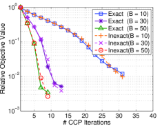
(b) Relative objective values w.r.t. outer iterations.

Figure 1: Convergence of Inexact FGM and Exact FGM on the synthetic dataset.

First, from Figure 1(a), for each comparison method, the function value sharply decreases at some iterations where an active constraint is added. For the Exact FGM, more APG iterations are required for the tolerance $\epsilon_{in}=1.0\times 10^{-6}$. However, the function value does not show a significant decrease after several APG iterations. In contrast, from Figure 1(a), the Inexact FGM, which uses a relatively larger tolerance $\epsilon_{in}=1.0\times 10^{-3}$, requires much fewer APG iterations to achieve similar objective values as Exact FGM for the same parameter $B$. Particularly, from Figure 1(b), the Inexact FGM achieves similar objective values as Exact FGM after each outer iteration. According to these observations, on one hand, $\epsilon_{in}$ should be small enough such that the subproblem can be sufficiently optimized. On the other hand, a relatively large tolerance (e.g., $\epsilon_{in}=1.0\times 10^{-3}$) can greatly accelerate the convergence speed without degrading the performance.

Moreover, according to Figure 1(b), PROX-FGM with a large $B$ in general converges faster than with a small $B$. Generally, by using a large $B$, lower numbers of outer iterations and worst-case analyses are required, which is critical when dealing with Big Data. However, if $B$ is too large, some non-informative features may be mistakenly included, and the solution may not be exactly sparse.

8.2.2 Experiments on Small-Scale Synthetic Dataset

In this experiment, we evaluate the performance of different methods in terms of testing accuracies w.r.t. different numbers of selected features. Specifically, to obtain sparse solutions with different sparsities, we vary $C\in[0.001,0.007]$ for l1-SVM, $C\in$ [5e-3, 4e-2] for l1-LR and $\lambda_{1}\in$ [7.2e-4, 2.5e-3] for SGD-SLR. In contrast to these methods, we fix $C=10$ and choose even numbers in $\{2,4,...,60\}$ for $B$ to obtain different numbers of features. It can be seen that it is much easier for FGM to control the number of features being selected. Specifically, the testing accuracies and the number of recovered ground-truth features w.r.t. the number of selected features are reported in Figure 2(a) and Figure 2(b), respectively. The training times for different methods are listed in Figure 2(d).

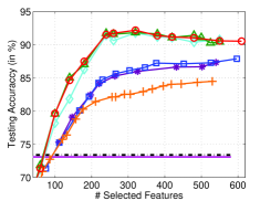
(a) Testing accuracy

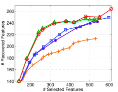
(b) Number of recovered features

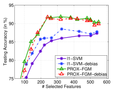
(c) De-biased results

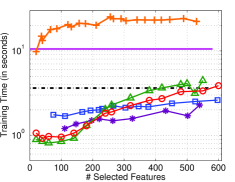
(d) Training time

Figure 2: Experimental results on the small dataset, where CD-SVM and CD-LR denote the results of standard SVM and LR with all features, respectively. The training time of MKL-FGM is about 1,500 seconds, which is up to 1,000 times slower than APG solver. We did not report it in the figures due to presentation issues.

For convenience of presentation, let $m_{s}$ and $m_{g}$ be the number of selected features and the number of ground-truth features, respectively. From Figure 2(a) and Figure 2(b), FGM-based methods demonstrate better testing accuracy than all $\ell_{1}$-methods when $m_{s}>100$. Correspondingly, from Figure 2(b), with the same number of selected features, FGM-based methods include more ground-truth features than $\ell_{1}$-methods when $m_{s}$$\geq$100. SGD-SLR shows the worst testing accuracy among the compared methods and recovers the least number of ground-truth features.

One of the possible reasons for the inferior performance of the $\ell_{1}$-methods, as mentioned in the Introduction section, is the solution bias caused by the $\ell_{1}$-regularization. To demonstrate this, we do retraining to reduce the bias using CD-SVM with $C=20$ with the selected features. Then, we do the prediction using the de-biased models. The results are reported in Figure 2(c), where l1-SVM-debias and PROX-FGM-debias denote the de-biased counterparts of l1-SVM and PROX-FGM, respectively. In general, if there was no feature selection bias, both FGM and l1-SVM should have similar testing accuracies as their de-biased counterparts. However, from Figure 2(c), l1-SVM-debias in general has much better testing accuracy than l1-SVM, while PROX-FGM has similar or even better testing accuracy than PROX-FGM-debias and l1-SVM-debias. These observations indicate that 1) the solution bias indeed exists in $\ell_{1}$-methods and affects the feature selection performance, and 2) FGM can reduce the feature selection bias.

From Figure 2(d), on this small-scale dataset, PROX-FGM and PROX-SLR achieve comparable efficiency as the LIBlinear solver. In contrast, SGD-SLR, which is a typical stochastic gradient method, spends the longest time training. This observation indicates that the SGD-SLR method may not be suitable for small-scale problems. Last, as reported in the caption of Figure 2(d), PROX-FGM and PROX-SLR are up to 1,000 times faster than MKL-FGM using the SimpleMKl solver. The reason for this is that SimpleMKl uses the subgradient method to address the non-smooth optimization problem with $n$ variables, while the subproblem is solved in the primal problem w.r.t. a small number of selected variables in PROX-FGM and PROX-SLR.

Last, from Figure 2, if the number of selected features is small ($m_{s}<100$), the testing accuracy is worse than CD-SVM and CD-LR with all features. However, if a sufficient number ($m_{s}>200$) of features are selected, the testing accuracy is much better than CD-SVM and CD-LR with all features, which verifies the importance of feature selection.

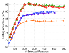
(a) Testing accuracy

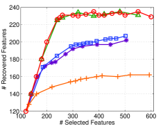
(b) Number of recovered features

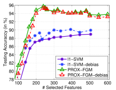
(c) De-biasing effect of FGM

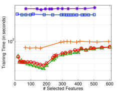
(d) Training time

Figure 3: Performance comparison on the large-scale synthetic dataset.

8.2.3 Experiments on Large-scale Synthetic Dataset

To demonstrate the scalability of FGM, we conduct an experiment on a large-scale synthetic dataset, namely, ${{\bf X}}\in{\mathbb{R}}^{8,192\times 65,536}$. Here, we do not include the comparisons with MKL-FGM due to its high computational cost. For PROX-FGM and PROX-SLR, we follow their experimental settings above. For l1-SVM and l1-LR, we vary $C\in[0.001,0.004]$ and $C\in[0.005,0.015]$, respectively, to determine the number of features to be selected. The testing accuracy, the number of recovered ground-truth features, the de-biased results and the training time of the compared methods are reported in Figure 3(a), 3(b), 3(c) and 3(d), respectively.

From Figure 3(a), 3(b) and 3(c), both PROX-FGM and PROX-SLR outperform l1-SVM, l1-LR and SGD-SLR in terms of both testing accuracy and the number of recovered ground-truth features. From Figure 3(d), PROX-FGM and PROX-SLR show better training efficiencies than the coordinate based methods (namely, LIBlinear) and the SGD based method (namely, SGD-SLR). Basically, FGM solves a sequence of small optimization problems with $O(ntB)$ cost and spends only a small number of iterations to do the worst-case analysis with $O(mn)$ cost. In contrast, the $\ell_{1}$-methods may take many iterations to converge, and each iteration takes $O(mn)$ cost. On this large-scale dataset, SGD-SLR shows a faster training speed than LIBlinear. However, it has a highly inferior performance in terms of testing accuracy compared to the LIBlinear solver.

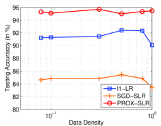
(a) Testing accuracy

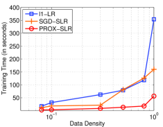
(b) Training time

Figure 4: Performance comparison on the synthetic dataset ($n=8,192$, $m=65,536$) with different data densities in $\{0.08,0.1,0.3,0.5,0.8,1\}$.

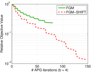
(a) Synthetic dataset ($b=4$)

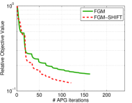
(b) astro-ph

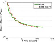
(c) real-sim

Figure 5: Relative objective values regarding each APG iteration, where $b=4$ in the caption of Figure 5(a) denotes the ground-truth shift of the hyperplane from the origin.

In LIBlinear, the efficiency has been improved by taking advantage of the data sparsity. Considering this, we investigate the sensitivity of the referred methods to the data density. To this end, we generate datasets of different data densities by sampling the entries from ${\bf X}^{8,192\times 65,656}$ with a sampling rate in $\{0.08,0.1,0.3,0.5,0.8,1\}$ and study the influence of the data density on different learning algorithms. For FGM, only the logistic loss is studied (namely, PROX-SLR). We keep the default experimental settings for PROX-SLR and watchfully vary $C\in[0.008,5]$ for l1-LR and $\lambda_{1}\in[\text{9.0e-4, 3e-3}]$ for SGD-SLR. For the sake of brevity, we only report the best accuracy obtained among all parameters and the corresponding training time of l1-LR, SGD-SLR and PROX-SLR in Figure 4.

From Figure 4(a), under different data densities, PROX-SLR always outperforms l1-SVM and SGD-SLR in terms of the best accuracy. From Figure 4(b), l1-SVM shows comparable efficiency with PROX-SLR on datasets of low data density. However, on relatively denser datasets, PROX-SLR is much more efficient than l1-SVM, which indicates that FGM has a better scalability than l1-SVM on dense data.

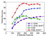
(a) Synthetic dataset ($b=4$)

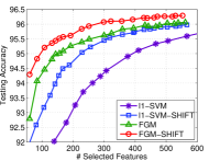
(b) astro-ph

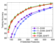
(c) real-sim

Figure 6: Testing accuracies of different methods on the three datasets.

8.3 Feature Selection with Shift Consideration

In this section, we study the effectiveness of the shift version of FGM (denoted by FGM-SHIFT) on a synthetic dataset and two real-world datasets, namely, real-sim and astro-ph. We follow the data generation procedure in Section 7.1 to generate the synthetic dataset except that we include a shift term $b$ for the hyperplane when generating the output ${\bf y}$. Specifically, we produce ${\bf y}$ by ${\bf y}=\text{sign}({\bf X}{\bf w}-b{\bf 1})$ where $b=4$. The shift version of $\ell_{1}$-SVM by LIBlinear (denoted by l1-SVM-SHIFT) is adopted as the baseline. In Figure 5, we report the relative objective values of FGM and FGM-SHIFT w.r.t. the APG iterations on three datasets. In Figure 6, we report the testing accuracy versus different numbers of selected features.

From Figure 5, FGM-SHIFT indeed achieves much lower objective values than FGM on the synthetic dataset and the astro-ph dataset, which demonstrates the effectiveness of FGM-SHIFT. On the real-sim dataset, FGM and FGM-SHIFT achieve similar objective values, which indicates that the shift term on real-sim is not significant. As a result, FGM-SHIFT may not significantly improve the testing accuracy.

From Figure 6, on the synthetic dataset and astro-ph dataset, FGM-SHIFT shows significantly better testing accuracy than the baseline methods, which coincides with the better objective values of FGM-SHIFT in Figure 5. l1-SVM-SHIFT also shows better testing accuracy than l1-SVM, which verifies the importance of shift consideration for l1-SVM. However, on the real-sim dataset, the methods with shift show similar or even inferior performance over the methods without shift consideration, which indicates that the shift of the hyperplane from the origin is not significant on the real-sim dataset. Last, FGM and FGM-SHIFT are always better than the counterparts of l1-SVM.

8.4 Performance Comparison on Real-World Datasets

In this section, we conduct three experiments to compare the performance of FGM with the referred baseline methods on real-world datasets. First, in Section 8.4.1, we compare the performance of different methods on six real-world datasets. Second, we study the de-biased results in Section 8.4.2. Last, we conduct a sensitivity study of parameters for FGM in Section 8.4.3.

8.4.1 Experimental Results on Real-World Datasets

On real-world datasets, the number of ground-truth features is unknown. We only report the testing accuracy versus different numbers of selected features. For FGM, we fix $C=10$, and vary $B\in\{2,4,...,60\}$ to select different numbers of features. For the $\ell_{1}$-methods, we watchfully vary the regularization parameter to select different numbers of features. The ranges of $C$ and $\lambda_{1}$ for $\ell_{1}$-methods are listed in Table 1.

The testing accuracy and training time for different methods versus the number of selected features are reported in Figure 7 and Figure 8, respectively. From Figure 7, on all datasets, FGM (including PROX-FGM, PROX-SLR and MKL-FGM) obtains comparable or better performance than the $\ell_{1}$-methods in terms of testing accuracy within 300 features. Particularly, FGM shows a much better testing accuracy than $\ell_{1}$-methods on five of the studied datasets, namely, epsilon, real-sim, rcv1.binary, Arxiv astro-ph and news20.

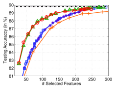
(a) epsilon

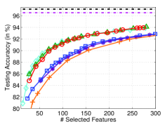
(b) real-sim

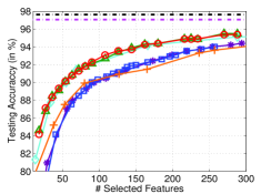
(c) rcv1

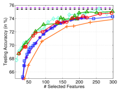
(d) news20

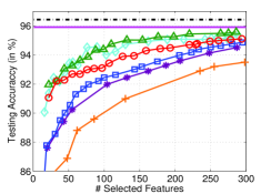
(e) astro-ph

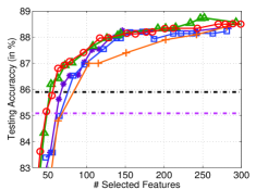
(f) kddb

Figure 7: Testing accuracies on various datasets.

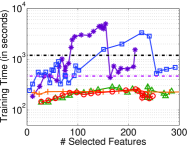
(a) epsilon

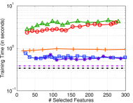
(b) real-sim

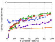
(c) rcv1

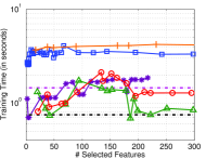
(d) news20

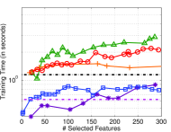
(e) physic

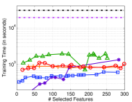
(f) kddb

Figure 8: Training times on various datasets.

From Figure 8, PROX-FGM and PROX-SLR show competitive training efficiency with the $\ell_{1}$-methods. Particularly, on the large-scale dense epsilon dataset, PROX-FGM and PROX-SLR are much more efficient than the LIBlinear $\ell_{1}$-solvers. For SGD-SLR, although it demonstrates comparable training efficiency as PROX-FGM and PROX-SLR, it attains a much worse testing accuracy. In summary, FGM-based methods in general obtain better feature subsets with competitive training efficiency as the considered baselines on real-world datasets.

8.4.2 De-biasing Effect of FGM

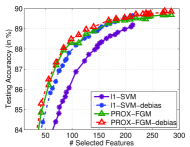
(a) epsilon

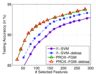
(b) real-sim

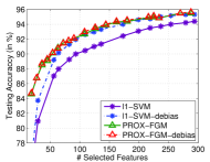
(c) rcv1

Figure 9: De-biased results on real-world datasets.

In this experiment, we demonstrate the de-biasing effect of FGM on three real-world datasets, namely, epsilon, real-sim and rcv1. Here, only the squared hinge loss (namely, PFOX-FGM) is studied. The de-biased results are reported in Figure 9, where PROX-FGM-debias and l1-SVM-debias denote the de-biased results of PROX-FGM and l1-SVM, respectively.

From Figure 9, l1-SVM-debias shows much better results than l1-SVM indicating that a feature selection bias issue exists in l1-SVM on these real-world datasets. In contrast, PROX-FGM achieves close or even better results compared with its de-biased counterparts, which verifies that PROX-FGM itself can reduce the feature selection bias. Moreover, on these datasets, FGM shows better testing accuracy than the de-biased l1-SVM, namely, l1-SVM-debias, which indicates that the features selected by FGM are more relevant than those obtained by l1-SVM due to the reduction of feature selection bias.

8.4.3 Sensitivity Study of Parameters

In this section, we conduct a sensitivity study of parameters for PROX-FGM. There are two parameters in FGM, namely, the sparsity parameter $B$ and the regularization parameter $C$. In these experiments, we study the sensitivity of these two parameters on real-sim and astro-ph datasets. l1-SVM is adopted as the baseline.

In the first experiment, we study the sensitivity of $C$. FGM with suitable $C$ can reduce the feature selection bias. However, if $C$ is too large, overfitting may occur. To demonstrate this, we test $C\in\{0.5,5,50,500\}$. The testing accuracy of FGM under different $C$’s is reported in Figure 10. From Figure 10, the testing accuracy with a small $C$ is worse in general than that with a large $C$. The reason for this is that, when $C$ is small, feature selection bias may occur due to an underfitting problem. However, when $C$ is sufficiently large, increasing $C$ may not necessarily improve the performance. More critically, if $C$ is too large, an overfitting problem may occur. For example, on the astro-ph dataset, FGM with $C=500$ performs much worse in general than FGM with $C=5$ and $C=50$. An important observation is that, on both datasets, FGM with different $C$’s generally performs better than the l1-SVM.

(a) real-sim

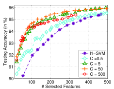
(b) astro-ph

Figure 10: Sensitivity of the parameter $C$ for FGM on real-sim and astro-ph datasets.

Recall that a large $C$ may lead to slower convergence speeds due to an increase in the Lipschitz constant of $F(\mbox{{\boldmath$\omega$}},b)$. In practice, we suggest choosing $C$ in the range of $[1,100]$. In Section 8.4, we have set $C=10$ for all datasets. In this setting, FGM has demonstrated superb performance over the competing methods. In contrast, choosing the regularization parameter for $\ell_{1}$-methods is more difficult. Therefore, FGM is convenient for performing model selection.

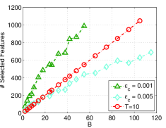
(a) $\#$ Selected Features Versus $B$

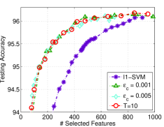
(b) Testing Accuracy Versus $B$

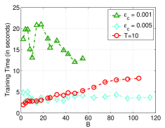
(c) Training Time (in seconds)

Figure 11: Sensitivity of the parameter $B$ for FGM on astro-ph dataset, where FGM is stopped once $(F(\mbox{{\boldmath$\omega$}}_{t-1},b)-F(\mbox{{\boldmath$\omega$}}_{t},b))/F(\mbox{{\boldmath$\omega$}}_{0},b)\leq\epsilon_{c}$.

In the second experiment, we study the sensitivity of parameter $B$ for FGM under two stopping conditions: (1) when the condition $(F(\mbox{{\boldmath$\omega$}}_{t-1},b)-F(\mbox{{\boldmath$\omega$}}_{t},b))/F(\mbox{{\boldmath$\omega$}}_{0},b)\leq\epsilon_{c}$ is achieved and (2) when a maximum $T$ iterations is achieved where $T=10$. Here, we test two values of $\epsilon_{c}$, namely, $\epsilon_{c}=0.005$ and $\epsilon_{c}=0.001$. The number of selected features, the testing accuracy and the training time versus different $B$ values are reported in Figure 11(a), 11(b) and 11(c), respectively.

In Figure 11(a), given the number of selected feature $\#~{}\text{features}$, the number of required iterations is approximately $\lceil\frac{\#~{}\text{features}}{B}\rceil$ under the first stopping criterion. In this sense, FGM with $\epsilon_{c}=0.001$ takes more than 10 iterations to terminate and thus will choose more features. As a result, it needs more time for optimization with the same $B$, as shown in Figure 11(c). In contrast, FGM with $\epsilon_{c}=0.005$ requires fewer iterations (smaller than 10 when $B>20$). Surprisingly, as shown in Figure 11(b), FGM with fewer iterations (where $\epsilon_{c}=0.005$ or $T=10$) obtains a similar testing accuracy as FGM with $\epsilon_{c}=0.001$, but shows much better training efficiency. This observation indicates that we can set a small number outer iterations (for example $5\leq T\leq 20$) to trade-off the training efficiency and the feature selection performance.

(a) Training Time (in seconds) Versus $B$

(b) Testing Accuracy Versus $B$

Figure 12: Sensitivity of the parameter $B$ for FGM on astro-ph dataset. Given a parameter $B$, we stop FGM once 400 features are selected.

In the third experiment, we study the influence of the parameter $B$ on the performance of FGM on the astro-ph dataset. Specifically, we stop FGM once 400 features are selected with different $B$’s. The training time and testing accuracy w.r.t. different $B$’s are shown in Figure 12(a) and 12(b), respectively.

From Figure 12(a), choosing a large $B$ in general leads to better training efficiency. Particularly, FGM with $B=40$ is approximately 200 times faster than FGM with $B=2$. Recall that active-set methods in (Roth and Fischer, 2008; Bach, 2009) can be considered as special cases of FGM with $B=1$. Accordingly, we can conclude that FGM with a properly selected $B$ can be much faster than active-set methods Roth and Fischer (2008); Bach (2009). However, it should be pointed that, if $B$ is too large, the performance may degrade. For instance, if we choose $B=400$, the testing accuracy dramatically degrades, which indicates that the selected 400 features are not the optimal ones. In summary, choosing a suitable $B$ (e.g., $B\leq 100$) can much improve the efficiency while maintaining promising generalization performance.

8.5 Ultrahigh Dimensional Feature Selection via Nonlinear Feature Mapping

In this experiment, we compare the efficiency of FGM and $\ell_{1}$-SVM on nonlinear feature selection with polynomial feature mappings on two medium dimensional datasets and a high dimensional dataset. The comparison methods are denoted by PROX-PFGM, PROX-PSLR and l1-PSVM. The details of the studied datasets are shown in Table 2, where $m_{Poly}$ denotes the dimension of the polynomial mappings and $\gamma$ is the polynomial kernel parameter used in this experiment. The mnist38 dataset consists of the digital images of $3$ and $8$ from the mnist dataset. For the kddb dataset, we only use the first $10^{6}$ instances. Last, we change the parameter $C$ for l1-PSVM to obtain different numbers of features.

Dataset	$m$	$m_{Poly}$	$n_{train}$	$n_{test}$	$\gamma$
mnist38	784	$O(10^{5})$	40,000	22,581	4.0
real-sim	20,958	$O(10^{8})$	32,309	40,000	8.0
kddb	4,590,807	$O(10^{14})$	$1000,000$	748,401	4.0

Table 2: Details of the datasets using polynomial feature mappings.

(a) mnist38

(b) real-sim

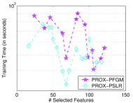
(c) kddb

Figure 13: Training times of different methods on nonlinear feature selection using polynomial mappings.

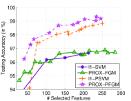
(a) mnist38

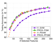
(b) real-sim

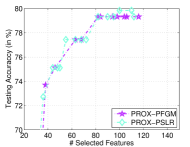
(c) kddb

Figure 14: Testing accuracies of different methods on nonlinear feature selection using polynomial mappings.

The training time and testing accuracy on different datasets are reported in Figure 13 and 14, respectively. Both PROX-PFGM and l1-PSVM can address the two medium dimensional problems. However, PROX-PFGM shows much better efficiency than l1-PSVM. Moreover, l1-PSVM is unfeasible on the kddb dataset due to the ultrahigh dimensionality. Particularly, l1-PSVM needs more than 1 TB of memory to store a dense ${\bf w}$, which is unfeasible for a common PC. Conversely, this difficulty can be effectively addressed by FGM. Specifically, PROX-PFGM completes the training within 1000 seconds.

From the figures, the testing accuracy on the mnist38 dataset with polynomial mapping is much better than that of linear methods, which demonstrates the usefulness of the nonlinear feature expansions. On the real-sim and kddb datasets however, the performance with polynomial mapping does not show significant improvements. A possible reason is that these two datasets are linearly separable.

8.6 Experiments for Group Feature Selection

In this section, we study the performance of the proposed methods for group feature selection on a synthetic dataset and two real-world datasets. Here, only the logistic loss is studied since it has been widely used for group feature selection on classification tasks (Roth and Fischer, 2008; Liu and Ye, 2010). To demonstrate the sensitivity of the parameter $C$ to FGM, we vary $C$ to select different numbers of groups under the stopping tolerance $\epsilon_{c}=0.001$. For each $C$, we test $B\in\{2,5,8,10\}$. The tradeoff parameter $\lambda$ in SLEP is chosen from $[0,1]$, where a larger lambda leads to more sparse solutions (Liu and Ye, 2010). Specifically, we set $\lambda$ in $[0.002,0.700]$ for FISTA and ACTIVE and set $\lambda$ in $[0.003,0.1]$ for BCD.

8.6.1 Synthetic Experiments on Group Feature Selection

In the synthetic experiment, we generate a random matrix ${{\bf X}}\in{\mathbb{R}}^{4,096\times 400,000}$, where each entry follows the i.i.d. Gaussian distribution $\mathcal{N}(0,1)$. After, we directly group the 400,000 features into 40,000 groups of equal size (Jenatton et al., 2011b), namely, each feature group contains 10 features. We randomly choose $100$ groups as the ground-truth informative groups. Specifically, we generate a sparse vector ${\bf w}$ where only the entries of the selected groups are nonzero values sampled from the i.i.d. Gaussian distribution $\mathcal{N}(0,1)$. Last, we produce the output labels by ${\bf y}=\text{sign}({{\bf X}}{\bf w})$. We generate 2,000 testing points in the same manner.

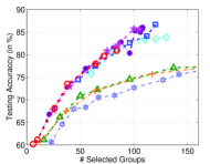
(a) Testing accuracy

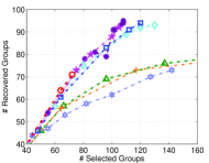
(b) Recovered features

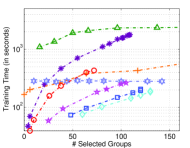
(c) Training time

Figure 15: Results of group feature selection on the synthetic dataset.

The testing accuracy, training time and number of recovered ground-truth groups are reported in Figure 15(a), 15(b) and 15(c), respectively. Here, only the results within 150 groups are included since we only have 100 informative ground-truth groups. From Figure 15(a), FGM achieves better testing accuracy than FISTA, BCD and UFO-MKL. The reason for this is that FGM can reduce the group feature selection bias. From Figure 15(c), in general, FGM is much more efficient than FISTA and BCD. Interestingly, the active-set method (ACTIVE) also shows good testing accuracy compared with FISTA and BCD. However, from Figure 15(c), its efficiency is limited since it only includes one element per iteration. Accordingly, when selecting a large number of groups on Big Data, the computational cost becomes unbearable. For UFO-MKL, although its training speed is fast, its testing accuracy is generally worse than others. Last, with a fixed $B$ for FGM, the number of selected groups will increase when $C$ becomes large. This is because, with a larger $C$, one places more importance on the training errors. Accordingly, more groups are required to achieve lower empirical errors.

Dataset	$m$	$n_{train}$	Size of training set (GB)			$n_{test}$	Size of testing set(GB)
			Linear	ADD	HIK		Linear	ADD	HIK
aut	20,707	40, 000	0.027	0.320	0.408	22,581	0.016	0.191	0.269
rcv1	47,236	677,399	0.727	8.29	9.700	20,242	0.022	0.256	0.455

Table 3: Details of the datasets used for HIK kernel feature expansion and Additive kernel feature expansion. For HIK kernel feature expansion, each original feature is represented by a group of 100 features, while for Additive kernel feature expansion, each original feature is represented by a group of 11 features.

8.6.2 Experiments on Real-World Datasets

In this section, we verify the effectiveness of FGM for group feature selection on two real-world datasets, namely, aut-avn and rcv1. In real-applications, the group prior of features comes in different ways. In this paper, we produce the feature groups using the explicit kernel feature expansions (Wu, 2012; Vedaldi and Zisserman, 2010), where each original feature is represented by a group of approximated features. Such expansion can vastly improve the training efficiency of kernel methods while maintaining good approximation performance in many applications, such as in computer vision (Wu, 2012). For simplicity, we only study the HIK kernel expansion (Wu, 2012) and the additive Gaussian kernel expansion (Vedaldi and Zisserman, 2010). In the experiments, for fair comparison, we pre-generate the explicit features for two datasets. The details of the two datasets and the feature expansions are listed Table 3. We can observe that, after feature expansion, the storage requirement dramatically increases. Figure 16 and 17 report the testing accuracy and training time of different methods, respectively.

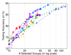
(a) aut-ADD

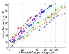
(b) rcv1-ADD

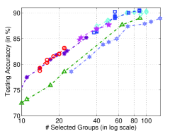
(c) aut-HIK

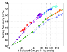
(d) rcv1-HIK

Figure 16: Testing accuracies on group feature selection tasks. The groups are generated by HIK or additive feature mappings. The results of BCD on aut-HIK is not reported due to the heavy computational cost.

From Figure 16, FGM and the active set method achieve superior performance over FISTA, BCD and UFO-MKL in terms of testing accuracy. Moreover, from Figure 17, FGM has much better efficiency than the active set method. It is worth mentioning that, due to the unbearable storage requirement, the feature expansion cannot be explicitly stored when dealing with ultrahigh-dimensional Big Data. Accordingly, FISTA and BCD, which require the explicit presentation of data, cannot work in such cases. However, the proposed feature generating paradigm can effectively address this computational issue since it only involves a sequence of small-scale optimization problems.

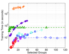
(a) aut-ADD

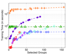
(b) rcv1-ADD

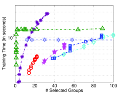
(c) aut-HIK

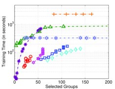
(d) rcv1-HIK

Figure 17: Training times on group feature selections.

9 Conclusions

In this paper, an adaptive feature scaling (AFS) scheme has been proposed to select the most informative features by introducing a feature scaling vector ${\bf d}\in[0,1]^{p}$ into the input features. To explicitly control the sparsity, we impose an $\ell_{1}$-norm constraint $||{\bf d}||_{1}\leq B$ on ${\bf d}$, where $B$ represents the least number of features to be selected. To address the resultant non-convex problem, we first transform it to a convex SIP problem and then propose a Feature Generating Machine (FGM) to solve it. FGM iteratively includes a group of informative features/groups and then solves a much reduced MKL subproblem. FGM has been extended to solve general MKL problems with additive kernels. The global convergence of FGM has been proved.

Compared with $\ell_{1}$-norm methods and other existing feature selection methods, FGM has two major advantages. First, with the separate control of the complexity and sparsity, the feature selection bias of $\ell_{1}$-norm methods can be greatly reduced by FGM with proper stopping conditions. Second, since only a small subset of features or kernels are involved in the subproblem optimization, FGM is particularly suitable for the ultrahigh-dimensional feature selection task. Furthermore, to make FGM scalable to Big Data, we propose to solve the primal form of the subproblem using a modified APG method. Due to the new optimization scheme, some efficient cache techniques are also developed to improve the training efficiency. Accordingly, FGM can efficiently tackle ultrahigh-dimensional Big Data for which most of the existing methods are unfeasible. It is worth mentioning that, by avoiding storing all the kernels with explicit kernel feature expansions, FGM vastly reduces the unbearable memory demands of general MKL learning tasks with many kernels. Thereafter, many intractable tasks using previous MKL methods now become feasible.

Last, comprehensive experiments have been conducted to verify the performance of the proposed methods on both linear feature selection and group feature selection tasks. Extensive experiments on synthetic datasets and real-world datasets have demonstrated that FGM archives superior performance compared with the baseline methods in terms of testing accuracy and training efficiency.

In this paper, the proposed methods have tackled Big Data problems with a million training examples ($O(10^{7})$) and 100 trillion features ($O(10^{14})$). Recall that the subproblem of FGM can be possibly solved through SGD methods. In the future, we will explore SGD methods to further improve the training efficiency for bigger data of ultra-large size where $n$ is in the billion or trillion scale.

Appendix A. Proof of Theorem 3

Proof  The proof parallels the results in (Bach et al., 2004) and uses the conic duality theory. Let $\Omega(\mbox{{\boldmath$\omega$}})=\frac{1}{2}\left({\|\mbox{{\boldmath$\omega$}}_{h}\|}{}\right)^{2}$ and define the cone $\mathcal{Q}_{B}=\{({\bf u},v)\in{\mathbb{R}}^{B+1},\|{\bf u}\|_{2}\leq v\}$. Furthermore, let $z_{h}=\|\mbox{{\boldmath$\omega$}}_{h}\|$, we have $\Omega(\mbox{{\boldmath$\omega$}})=\frac{1}{2}\left(\sum_{h=1}^{t}{\|\mbox{{\boldmath$\omega$}}_{t}\|}\right)^{2}=\frac{1}{2}z^{2}$ with $z=\sum_{h=1}^{t}{z_{h}}{}$. Apparently, we have $z_{h}\geq 0$ and $z\geq 0$. Last, problem (31) can be transformed into the following problem:

$$\min\limits_{z,\mbox{{\boldmath$\omega$}}} \frac{1}{2}z^{2}+P(\mbox{{\boldmath$\omega$}},b),~{}~{}~{}\text{s.t.}~{}\sum\limits_{h=1}^{t}{z_{h}}{}\leq z,~{}~{}~{}(\mbox{{\boldmath$\omega$}}_{t},z_{h})\in\mathcal{Q}_{B},$$

where $\mbox{{\boldmath$\omega$}}=[\mbox{{\boldmath$\omega$}}_{1}^{\prime},...,\mbox{{\boldmath$\omega$}}_{t}^{\prime}]^{\prime}$. The Lagrangian function of (31) regarding the squared hinge loss can be written as follows:

$${\mathcal{L}}(z,\mbox{{\boldmath$\omega$}},\mbox{{\boldmath$\xi$}},b,\mbox{{\boldmath$\alpha$}},\gamma,\mbox{{\boldmath$\zeta$}},\mbox{{\boldmath$\varpi$}})$$

$$\!=\! \!\frac{1}{2}z^{2}+\frac{C}{2}\sum_{i=1}^{n}\xi_{i}^{2}-\sum_{i=1}^{n}\alpha_{i}\left(y_{i}(\sum{}\mbox{{\boldmath$\omega$}}_{h}^{\prime}{\bf x}_{ih}-b)-1+\xi_{i}\right)+\gamma(\sum\limits_{h=1}^{t}{z_{h}}-z)-\sum\limits_{h=1}^{t}(\mbox{{\boldmath$\zeta$}}_{h}^{\prime}\mbox{{\boldmath$\omega$}}_{h}+\varpi_{h}z_{h}),$$

where $\alpha$, $\gamma$, $\mbox{{\boldmath$\zeta$}}_{t}$ and $\varpi_{t}$ are the Lagrangian dual variables to the corresponding constraints. The KKT condition can be expressed as follows:

$$\begin{array}[]{ll}\nabla_{z}{\mathcal{L}}=z-\gamma=0&\Rightarrow z=\gamma;\\ \nabla_{z_{h}}{\mathcal{L}}={\gamma}{}-\varpi_{h}=0&\Rightarrow\varpi_{h}={\gamma}{};\\ \nabla_{\mbox{{\boldmath$\omega$}}_{h}}{\mathcal{L}}=-\sum_{i=1}^{n}\alpha_{i}y_{i}{\bf x}_{ih}-\mbox{{\boldmath$\zeta$}}_{h}=0&\Rightarrow\mbox{{\boldmath$\zeta$}}_{h}=-\sum_{i=1}^{n}\alpha_{i}y_{i}{\bf x}_{ih};\\ \nabla_{\xi_{i}}{\mathcal{L}}=C\xi_{i}-\alpha_{i}=0&\Rightarrow\xi_{i}=\frac{\alpha_{i}}{C};\\ \|\mbox{{\boldmath$\zeta$}}_{h}\|\leq\varpi_{h}&\Rightarrow\|\mbox{{\boldmath$\zeta$}}_{h}\|\leq{\gamma}{};\\ \nabla_{b}{\mathcal{L}}=0&\Rightarrow\sum_{i=1}^{n}{\alpha_{i}}y_{i}=0.\end{array}$$

By substituting all the above results into (Appendix A. Proof of Theorem 3), we can obtain the following

$${{\mathcal{L}}(z,\mbox{{\boldmath$\omega$}},\mbox{{\boldmath$\alpha$}},\gamma,\mbox{{\boldmath$\zeta$}},\mbox{{\boldmath$\varpi$}})}=-\frac{1}{2}\gamma^{2}-\frac{1}{2C}\mbox{{\boldmath$\alpha$}}^{\prime}\mbox{{\boldmath$\alpha$}}+1^{\prime}\mbox{{\boldmath$\alpha$}}.$$

Hence the dual problem of the $\ell_{2,1}^{2}$-regularized problem regarding squared hinge loss can be written as follows:

$${\max\limits_{\gamma,\mbox{{\boldmath$\alpha$}}}} -\frac{1}{2}\gamma^{2}-\frac{1}{2C}\mbox{{\boldmath$\alpha$}}^{\prime}\mbox{{\boldmath$\alpha$}}+1^{\prime}\mbox{{\boldmath$\alpha$}}$$

$$s.t {}\Big{\|}\sum_{i=1}^{n}\alpha_{i}y_{i}{\bf x}_{ih}\Big{\|}\leq\gamma,~{}~{}{h=1,\cdots,t},$$

$$\sum_{i=1}^{n}{\alpha_{i}}y_{i}=0,\alpha_{i}\geq 0,~{}~{}{i=1,\cdots,n}.$$

Let $\theta=\frac{1}{2}\gamma^{2}+\frac{1}{2C}\mbox{{\boldmath$\alpha$}}^{\prime}\mbox{{\boldmath$\alpha$}}-\mbox{{\boldmath$\alpha$}}^{\prime}{\bf 1}$, $\mbox{{\boldmath$\omega$}}_{h}=\sum_{i=1}^{n}\alpha_{i}y_{i}{\bf x}_{ih}$ and $f(\mbox{{\boldmath$\alpha$}},{\bf d}_{h})=\frac{1}{2}{}\|\mbox{{\boldmath$\omega$}}_{h}\|^{2}+\frac{1}{2C}\mbox{{\boldmath$\alpha$}}^{\prime}\mbox{{\boldmath$\alpha$}}-\mbox{{\boldmath$\alpha$}}^{\prime}{\bf 1}$, we have the following

$${\max\limits_{\theta,\mbox{{\boldmath$\alpha$}}}} -\theta,$$

$$s.t f(\mbox{{\boldmath$\alpha$}},{\bf d}_{h})\leq\theta,~{}~{}{h=1,\cdots,t},$$

$$\sum_{i=1}^{n}{\alpha_{i}}y_{i}=0,\alpha_{i}\geq 0,~{}~{}{i=1,\cdots,n},$$

which indeed is in the form of problem (22) by letting ${\cal A}$ be the domain of $\alpha$. This completes the proof and brings the connection between the primal and dual formulation.

By defining $0\log(0)=0$, with the similar derivation above, we can obtain the dual form of (31) regarding the logistic loss. Let $\mbox{{\boldmath$\omega$}}=[\mbox{{\boldmath$\omega$}}_{1}^{\prime},...,\mbox{{\boldmath$\omega$}}_{t}^{\prime}]^{\prime}$, we have the following

$$\min\limits_{z,\mbox{{\boldmath$\omega$}}} \frac{1}{2}z^{2}+P(\mbox{{\boldmath$\omega$}},b),~{}~{}~{}\text{s.t.}~{}\sum\limits_{h=1}^{t}{z_{h}}{}\leq z,~{}~{}~{}(\mbox{{\boldmath$\omega$}}_{t},z_{h})\in\mathcal{Q}_{B}.$$ (52)

The Lagrangian function of (31) regarding logistic loss can be written as follows:

$${\mathcal{L}}(z,\mbox{{\boldmath$\omega$}},\mbox{{\boldmath$\xi$}},b,\mbox{{\boldmath$\alpha$}},\gamma,\mbox{{\boldmath$\zeta$}},\mbox{{\boldmath$\varpi$}})$$

$$= \frac{1}{2}z^{2}+C\sum_{i=1}^{n}\log(1+\exp(\xi_{i}))-\sum_{i=1}^{n}\alpha_{i}\left(y_{i}(\sum{}\mbox{{\boldmath$\omega$}}_{h}^{\prime}{\bf x}_{ih}-b)+\xi_{i}\right)+\gamma(\sum\limits_{h=1}^{t}{z_{h}}-z)-\sum\limits_{h=1}^{t}(\mbox{{\boldmath$\zeta$}}_{h}^{\prime}\mbox{{\boldmath$\omega$}}_{h}+\varpi_{h}z_{h}),$$

where $\alpha$, $\gamma$, $\mbox{{\boldmath$\zeta$}}_{t}$ and $\varpi_{t}$ are the Lagrangian dual variables to the corresponding constraints. The KKT condition can be expressed as follows:

$$\begin{array}[]{ll}\nabla_{z}{\mathcal{L}}=z-\gamma=0&\Rightarrow z=\gamma;\\ \nabla_{z_{h}}{\mathcal{L}}={\gamma}{}-\varpi_{h}=0&\Rightarrow\varpi_{h}={\gamma}{};\\ \nabla_{\mbox{{\boldmath$\omega$}}_{h}}{\mathcal{L}}=-\sum_{i=1}^{n}\alpha_{i}y_{i}{\bf x}_{ih}-\mbox{{\boldmath$\zeta$}}_{h}=0&\Rightarrow\mbox{{\boldmath$\zeta$}}_{h}=-\sum_{i=1}^{n}\alpha_{i}y_{i}{\bf x}_{ih};\\ \nabla_{\xi_{i}}{\mathcal{L}}=\frac{C\exp(\xi_{i})}{1+\exp(\xi_{i})}-\alpha_{i}=0&\Rightarrow\exp(\xi_{i})=\frac{\alpha_{i}}{C-\alpha_{i}};\\ \|\mbox{{\boldmath$\zeta$}}_{h}\|\leq\varpi_{h}&\Rightarrow\|\mbox{{\boldmath$\zeta$}}_{h}\|\leq{\gamma}{};\\ \nabla_{b}{\mathcal{L}}=0&\Rightarrow\sum_{i=1}^{n}{\alpha_{i}}y_{i}=0.\end{array}$$

By substituting all the above results into (Appendix A. Proof of Theorem 3), we obtain the following

$${{\mathcal{L}}(z,\mbox{{\boldmath$\omega$}},\mbox{{\boldmath$\alpha$}},\gamma,\mbox{{\boldmath$\zeta$}},\mbox{{\boldmath$\varpi$}})}=-\frac{1}{2}\gamma^{2}-\sum_{i=1}^{n}(C-\alpha_{i})\log({C-\alpha_{i}})-\sum_{i=1}^{n}\alpha_{i}\log({\alpha_{i}}).$$

The dual form of the $\ell_{2,1}^{2}$-regularized problem regarding logistic loss can be written as follows:

$${\max\limits_{\gamma,\mbox{{\boldmath$\alpha$}}}} -\frac{1}{2}\gamma^{2}-\sum_{i=1}^{n}(C-\alpha_{i})\log({C-\alpha_{i}})-\sum_{i=1}^{n}\alpha_{i}\log({\alpha_{i}})$$

s.t. $${}\Big{\|}\sum_{i=1}^{n}\alpha_{i}y_{i}{\bf x}_{ih}\Big{\|}\leq\gamma,~{}~{}{h=1,\cdots,t},$$

$$\sum_{i=1}^{n}{\alpha_{i}}y_{i}=0,\alpha_{i}\geq 0,~{}~{}{i=1,\cdots,n}.$$

Let $\theta=\frac{1}{2}\gamma^{2}+\sum_{i=1}^{n}(C-\alpha_{i})\log({C-\alpha_{i}})+\sum_{i=1}^{n}\alpha_{i}\log({\alpha_{i}})$, $\mbox{{\boldmath$\omega$}}_{h}=\sum_{i=1}^{n}\alpha_{i}y_{i}{\bf x}_{ih}$, $f(\mbox{{\boldmath$\alpha$}},{\bf d}_{h})=\frac{1}{2}{}\|\mbox{{\boldmath$\omega$}}_{h}\|^{2}+\sum_{i=1}^{n}(C-\alpha_{i})\log({C-\alpha_{i}})+\sum_{i=1}^{n}\alpha_{i}\log({\alpha_{i}})$, then we have the following

$${\max\limits_{\theta,\mbox{{\boldmath$\alpha$}}}} -\theta,$$ (54)

s.t. $$f(\mbox{{\boldmath$\alpha$}},{\bf d}_{h})\leq\theta,~{}~{}{h=1,\cdots,t},$$

$$\sum_{i=1}^{n}{\alpha_{i}}y_{i}=0,~{}~{}0\leq\alpha_{i}\leq C,~{}~{}{i=1,\cdots,n}.$$

Last, according to the KKT conditon, we can easily recover the dual variable $\alpha$ by $\alpha_{i}=\frac{C\exp(\xi_{i})}{1+\exp(\xi_{i})}$. This completes the proof.  

Appendix B. Proof of Theorem 4

The proof parallels the results in (Beck and Teboulle, 2009) and includes several lemmas. First, we define a one variable function $Q_{\tau_{b}}({\bf v},b,v_{b})$ w.r.t. $b$ as follows:

$$Q_{\tau_{b}}({\bf v},b,v_{b}) = P({\bf v},v_{b})+\langle\nabla_{b}P({\bf v},v_{b}),b-v_{b}\rangle+\frac{\tau_{b}}{2}\|b-v_{b}\|^{2},$$ (55)

where we abuse the operators $\langle,\rangle$ and $\|\cdot\|$ for convenience.

Lemma 5

$S_{\tau}({\bf u},{\bf v})=\arg\min_{\mbox{{\boldmath$\omega$}}}Q_{\tau}(\mbox{{\boldmath$\omega$}},{\bf v},v_{b})$ is the minimizer of problem (33) at point ${\bf v}$, if and only if there exists $g(S_{\tau}({\bf u},{\bf v}))\in\partial\Omega(S_{\tau}({\bf u},{\bf v}))$, the subgradient of $\Omega(\mbox{{\boldmath$\omega$}})$ at $S_{\tau}({\bf u},{\bf v})$, such that

$$g(S_{\tau}({\bf u},{\bf v}))+\tau(S_{\tau}({\bf u},{\bf v})-{\bf v})+\nabla P({\bf v})={\bf 0}.$$ (56)

Proof  The proof can be completed by the optimality condition of $Q_{\tau}(\mbox{{\boldmath$\omega$}},{\bf v},v_{b})$ w.r.t. $\omega$.  

Lemma 6

Let $S_{\tau}({\bf u},{\bf v})=\arg\min_{\mbox{{\boldmath$\omega$}}}Q_{\tau}(\mbox{{\boldmath$\omega$}},{\bf v},v_{b})$ be the minimizer of problem (33) at point ${\bf v}$, and $S_{\tau_{b}}(b)=\arg\min_{b}Q_{\tau_{b}}({\bf v},b,v_{b})$ be the minimizer of problem (55) at point $v_{b}$. Due to the line search in Algorithm 4, we have the following

$$F(S_{\tau}({\bf u},{\bf v}),v_{b})\leq Q_{\tau}(S_{\tau}({\bf u},{\bf v}),{\bf v},v_{b}).$$

$$P({\bf v},S_{\tau_{b}}(v_{b}))\leq Q_{\tau_{b}}({\bf v},S_{\tau_{b}}(v_{b}),v_{b}).$$

and

$$F(S_{\tau}({\bf u},{\bf v}),S_{\tau_{b}}(b))\leq Q_{\tau}(S_{\tau}({\bf u},{\bf v}),{\bf v},v_{b})+\langle\nabla_{b}P({\bf v},v_{b}),S_{\tau_{b}}(b)-v_{b}\rangle+\frac{\tau_{b}}{2}\|S_{\tau_{b}}(b)-v_{b}||^{2}.$$ (57)

Furthermore, for any $(\mbox{{\boldmath$\omega$}}^{\prime},b)^{\prime}$ we have the following

$$F(\mbox{{\boldmath$\omega$}},b)-F(S_{\tau}({\bf u},{\bf v}),S_{\tau_{b}}(b)) \geq \tau_{b}\langle S_{\tau_{b}}(b)-v_{b},v_{b}-b\rangle+\frac{\tau_{b}}{2}\|S_{\tau_{b}}(b)-v_{b}||^{2}$$ (58)

$$+\tau\langle S_{\tau}({\bf u},{\bf v})-{\bf v},{\bf v}-\mbox{{\boldmath$\omega$}}\rangle+\frac{\tau}{2}\|S_{\tau}({\bf u},{\bf v})-{\bf v}||^{2}.$$

Proof  We only prove the inequality (57) and (58). First, recall that in Algorithm 4, we update $\omega$ and $b$ separately. It follows that

$$F(S_{\tau}({\bf u},{\bf v}),S_{\tau_{b}}(b))$$

$$= \Omega(S_{\tau}({\bf u},{\bf v}))+P(S_{\tau}({\bf u},{\bf v}),S_{\tau_{b}}(v_{b}))$$

$$\leq \Omega(S_{\tau}({\bf u},{\bf v}))+Q_{\tau_{b}}(S_{\tau}({\bf u},{\bf v}),S_{\tau_{b}}(b),v_{b})$$

$$= \Omega(S_{\tau}({\bf u},{\bf v}))+P(S_{\tau}({\bf u},{\bf v}),v_{b})+\langle\nabla_{b}P({\bf v},v_{b}),S_{\tau_{b}}(b)-v_{b}\rangle+\frac{\tau_{b}}{2}\|S_{\tau_{b}}(b)-v_{b}||^{2}$$

$$= F(S_{\tau}({\bf u},{\bf v}),v_{b})+\langle\nabla_{b}P({\bf v},v_{b}),S_{\tau_{b}}(b)-v_{b}\rangle+\frac{\tau_{b}}{2}\|S_{\tau_{b}}(b)-v_{b}||^{2}$$

$$\leq Q_{\tau}(S_{\tau}({\bf u},{\bf v}),{\bf v},v_{b})+\langle\nabla_{b}P({\bf v},v_{b}),S_{\tau_{b}}(b)-v_{b}\rangle+\frac{\tau_{b}}{2}\|S_{\tau_{b}}(b)-v_{b}||^{2}.$$

This proves the inequality in (57).

Now we prove the inequality (58). First, since both $P(\mbox{{\boldmath$\omega$}},b)$ and $\Omega(\mbox{{\boldmath$\omega$}})$ are convex functions, we have the following

$$P(\mbox{{\boldmath$\omega$}},b)\geq P({\bf v},v_{b})+\langle\nabla P({\bf v}),\mbox{{\boldmath$\omega$}}-{\bf v}\rangle+\langle\nabla_{b}P({\bf v},v_{b}),b-v_{b}\rangle,$$

$$\Omega(\mbox{{\boldmath$\omega$}})\geq\Omega(S_{\tau}({\bf u},{\bf v}))+\langle\mbox{{\boldmath$\omega$}}-S_{\tau}({\bf u},{\bf v}),g(S_{\tau}({\bf g},{\bf v}))\rangle,$$

where $g(S_{\tau}({\bf u},{\bf v}))$ is the subgradient of $\Omega(\mbox{{\boldmath$\omega$}})$ at point $S_{\tau}({\bf u},{\bf v})$. Summing up the above inequalities, we obtain the following

$$F(\mbox{{\boldmath$\omega$}},b)$$

$$\geq P({\bf v},v_{b})+\langle\nabla P({\bf v}),\mbox{{\boldmath$\omega$}}-{\bf v}\rangle+\langle\nabla_{b}P({\bf v},v_{b}),b-v_{b}\rangle+\Omega(S_{\tau}({\bf u},{\bf v}))+\langle\mbox{{\boldmath$\omega$}}-S_{\tau}({\bf u},{\bf v}),g(S_{\tau}({\bf g},{\bf v}))\rangle.$$

In addition, we have the following

$$F(\mbox{{\boldmath$\omega$}},b)-\left(Q_{\tau}(S_{\tau}({\bf u},{\bf v}),{\bf v},v_{b})+\langle\nabla_{b}P({\bf v},v_{b}),S_{\tau_{b}}(b)-v_{b}\rangle+\frac{\tau_{b}}{2}\|S_{\tau_{b}}(b)-v_{b}||^{2}\right)$$ (60)

$$= P({\bf v},v_{b})+\langle\nabla P({\bf v}),\mbox{{\boldmath$\omega$}}-{\bf v}\rangle+\langle\nabla_{b}P({\bf v},v_{b}),b-v_{b}\rangle+\Omega(S_{\tau}({\bf u},{\bf v}))+\langle\mbox{{\boldmath$\omega$}}-S_{\tau}({\bf u},{\bf v}),g(S_{\tau}({\bf g},{\bf v}))\rangle,$$

$$-\left(Q_{\tau}(S_{\tau}({\bf u},{\bf v}),{\bf v},v_{b})+\langle\nabla_{b}P({\bf v},v_{b}),S_{\tau_{b}}(b)-v_{b}\rangle+\frac{\tau_{b}}{2}\|S_{\tau_{b}}(b)-v_{b}||^{2}\right)$$

$$= P({\bf v},v_{b})+\langle\nabla P({\bf v}),\mbox{{\boldmath$\omega$}}-{\bf v}\rangle+\langle\nabla_{b}P({\bf v},v_{b}),b-v_{b}\rangle+\Omega(S_{\tau}({\bf u},{\bf v}))+\langle\mbox{{\boldmath$\omega$}}-S_{\tau}({\bf u},{\bf v}),g(S_{\tau}({\bf g},{\bf v}))\rangle,$$

$$-\left(P({\bf v},v_{b})+\langle\nabla P({\bf v}),S_{\tau}({\bf u},{\bf v})-{\bf v}\rangle+\Omega(S_{\tau}({\bf u},{\bf v}))+\frac{\tau}{2}\|S_{\tau}({\bf u},{\bf v})-{\bf v}||^{2}+\langle\nabla_{b}P({\bf v},v_{b}),S_{\tau_{b}}(b)-v_{b}\rangle+\frac{\tau_{b}}{2}\|S_{\tau_{b}}(b)-v_{b}||^{2}\right)$$

$$= \langle\nabla P({\bf v})+g(S_{\tau}({\bf g},{\bf v})),\mbox{{\boldmath$\omega$}}-S_{\tau}({\bf u},{\bf v})\rangle-\frac{\tau}{2}\|S_{\tau}({\bf u},{\bf v})-{\bf v}||^{2}$$

$$+\langle\nabla_{b}P({\bf v},v_{b}),b-S_{\tau_{b}}(b)\rangle-\frac{\tau_{b}}{2}\|S_{\tau_{b}}(b)-v_{b}||^{2}.$$

With the relation $S_{\tau_{b}}(b)=b-\frac{\nabla_{b}P({\bf v},v_{b})}{\tau_{b}}$ and Lemma 5, we obtain the following

$$F(\mbox{{\boldmath$\omega$}},b)-F(S_{\tau}({\bf u},{\bf v}),S_{\tau_{b}}(b))$$

$$\geq F(\mbox{{\boldmath$\omega$}},b)-\left(Q_{\tau}(S_{\tau}({\bf u},{\bf v}),{\bf v},v_{b})+\langle\nabla_{b}P({\bf v},v_{b}),S_{\tau_{b}}(b)-v_{b}\rangle+\frac{\tau_{b}}{2}\|S_{\tau_{b}}(b)-v_{b}||^{2}\right).$$

$$\geq \langle\nabla P({\bf v})+g(S_{\tau}({\bf g},{\bf v})),\mbox{{\boldmath$\omega$}}-S_{\tau}({\bf u},{\bf v})\rangle-\frac{\tau}{2}\|S_{\tau}({\bf u},{\bf v})-{\bf v}||^{2}$$

$$+\langle\nabla_{b}P({\bf v},v_{b}),b-S_{\tau_{b}}(b)\rangle-\frac{\tau_{b}}{2}\|S_{\tau_{b}}(b)-v_{b}||^{2}.$$

$$= \tau\langle{\bf v}-S_{\tau}({\bf u},{\bf v}),\mbox{{\boldmath$\omega$}}-S_{\tau}({\bf u},{\bf v})\rangle-\frac{\tau}{2}\|S_{\tau}({\bf u},{\bf v})-{\bf v}||^{2}$$

$$+\tau_{b}\langle v_{b}-S_{\tau_{b}}(b),b-S_{\tau_{b}}(b)\rangle-\frac{\tau_{b}}{2}\|S_{\tau_{b}}(b)-v_{b}||^{2}.$$

$$= \tau\langle S_{\tau}({\bf u},{\bf v})-{\bf v},{\bf v}-\mbox{{\boldmath$\omega$}}\rangle+\frac{\tau}{2}\|S_{\tau}({\bf u},{\bf v})-{\bf v}||^{2}$$

$$+\tau_{b}\langle S_{\tau_{b}}(b)-v_{b},v_{b}-b\rangle+\frac{\tau_{b}}{2}\|S_{\tau_{b}}(b)-v_{b}||^{2}.$$

This completes the proof.  

Lemma 7

Let $L_{bt}=\sigma L_{t}$, where $\sigma>0$. Furthermore, let us define

$$\mu^{k}=F(\mbox{{\boldmath$\omega$}}^{k},b^{k})-F(\mbox{{\boldmath$\omega$}}^{*},b^{*}),$$

$$\mbox{{\boldmath$\nu$}}^{k}=\rho^{k}\mbox{{\boldmath$\omega$}}^{k}-(\rho^{k}-1)\mbox{{\boldmath$\omega$}}^{k-1}-\mbox{{\boldmath$\omega$}}^{*},$$

$$\upsilon^{k}=\rho^{k}b^{k}-(\rho^{k}-1)b^{k-1}-b^{*},$$

and then the following relation holds:

$$\frac{2(\rho^{k})^{2}\mu^{k}}{L^{k}}-\frac{(\rho^{k+1})^{2}\mu^{k+1}}{L^{k+1}}\geq\left(||\mbox{{\boldmath$\nu$}}^{k+1}||^{2}-||\mbox{{\boldmath$\nu$}}^{k}||^{2}\right)+\sigma\left((\upsilon^{k+1})^{2}-(\upsilon^{k})^{2}\right).$$ (61)

Proof  Notice that we have $\mbox{{\boldmath$\omega$}}^{k+1}=S_{\tau}({\bf u},{\bf v}^{k+1})$ and $b^{k+1}=S_{\tau_{b}}(v_{b}^{k+1})$. By applying Lemma 6, let $\mbox{{\boldmath$\omega$}}=\mbox{{\boldmath$\omega$}}^{k}$, ${\bf v}={\bf v}^{k+1},\tau=L^{k+1}$, $b=b^{k}$, $v_{b}=v_{b}^{k+1},\tau_{b}=L_{b}^{k+1}$, we have the following

$$2(\mu^{k}-\mu^{k+1}) \geq L^{k+1}\left(||\mbox{{\boldmath$\omega$}}^{k+1}-{\bf v}^{k+1}||^{2}+2\langle\mbox{{\boldmath$\omega$}}^{k+1}-{\bf v}^{k+1},{\bf v}^{k+1}-\mbox{{\boldmath$\omega$}}^{k}\rangle\right)$$

$$+L_{b}^{k+1}\left(||b^{k+1}-v_{b}^{k+1}||^{2}+2\langle b^{k+1}-v_{b}^{k+1},v_{b}^{k+1}-b^{k}\rangle\right).$$

Multiplying both sides by $(\rho^{k+1}-1)$, we obtain the following

$$2(\rho^{k+1}-1)(\mu^{k}-\mu^{k+1}) \geq L^{k+1}(\rho^{k+1}-1)\left(||\mbox{{\boldmath$\omega$}}^{k+1}-{\bf v}^{k+1}||^{2}+2\langle\mbox{{\boldmath$\omega$}}^{k+1}-{\bf v}^{k+1},{\bf v}^{k+1}-\mbox{{\boldmath$\omega$}}^{k}\rangle\right)$$

$$+L_{b}^{k+1}(\rho^{k+1}-1)\left(||b^{k+1}-v_{b}^{k+1}||^{2}+2\langle b^{k+1}-v_{b}^{k+1},v_{b}^{k+1}-b^{k}\rangle\right).$$

Also, let $\mbox{{\boldmath$\omega$}}=\mbox{{\boldmath$\omega$}}^{*}$, ${\bf v}={\bf v}^{k+1},\tau=L^{k+1}$, $b=b^{k}$, $v_{b}=v_{b}^{k+1}$, and $\tau_{b}=L_{b}^{k+1}$, we have the following

$$-2\mu^{k+1} \geq L^{k+1}\left(||\mbox{{\boldmath$\omega$}}^{k+1}-{\bf v}^{k+1}||^{2}+2\langle\mbox{{\boldmath$\omega$}}^{k+1}-{\bf v}^{k+1},{\bf v}^{k+1}-\mbox{{\boldmath$\omega$}}^{*}\rangle\right)$$

$$+L_{b}^{k+1}\left(||b^{k+1}-v_{b}^{k+1}||^{2}+2\langle b^{k+1}-v_{b}^{k+1},v_{b}^{k+1}-b^{*}\rangle\right).$$

Summing up the above two inequalities, we get the following

$$2\left((\rho^{k+1}-1)\mu^{k}-\rho^{k+1}\mu^{k+1}\right)$$

$$\geq L^{k+1}\left(\rho^{k+1}||\mbox{{\boldmath$\omega$}}^{k+1}-{\bf v}^{k+1}||^{2}+2\langle\mbox{{\boldmath$\omega$}}^{k+1}-{\bf v}^{k+1},\rho^{k+1}{\bf v}^{k+1}-(\rho^{k+1}-1)\mbox{{\boldmath$\omega$}}^{k}-\mbox{{\boldmath$\omega$}}^{*}\rangle\right)$$

$$+L_{b}^{k+1}\left(\rho^{k+1}||b^{k+1}-v_{b}^{k+1}||^{2}+2\langle b^{k+1}-v_{b}^{k+1},\rho^{k+1}v_{b}^{k+1}-(\rho^{k+1}-1)b^{k}-b^{*}\rangle\right).$$

Multiplying both sides by $\rho^{k+1}$, we obtain the following

$$2\left(\rho^{k+1}(\rho^{k+1}-1)\mu^{k}-(\rho^{k+1})^{2}\mu^{k+1}\right)$$

$$\geq L^{k+1}\left((\rho^{k+1})^{2}||\mbox{{\boldmath$\omega$}}^{k+1}-{\bf v}^{k+1}||^{2}+2\rho^{k+1}\langle\mbox{{\boldmath$\omega$}}^{k+1}-{\bf v}^{k+1},\rho^{k+1}{\bf v}^{k+1}-(\rho^{k+1}-1)\mbox{{\boldmath$\omega$}}^{k}-\mbox{{\boldmath$\omega$}}^{*}\rangle\right)$$

$$+L_{b}^{k+1}\left((\rho^{k+1})^{2}||b^{k+1}-v_{b}^{k+1}||^{2}+2\rho^{k+1}\langle b^{k+1}-v_{b}^{k+1},\rho^{k+1}v_{b}^{k+1}-(\rho^{k+1}-1)b^{k}-b^{*}\rangle\right).$$

Since $(\rho^{k})^{2}=(\rho^{k+1})^{2}-\rho^{k+1}$, it follows that

$$2\left((\rho^{k})^{2}\mu^{k}-(\rho^{k+1})^{2}\mu^{k+1}\right)$$

$$\geq L^{k+1}\left((\rho^{k+1})^{2}||\mbox{{\boldmath$\omega$}}^{k+1}-{\bf v}^{k+1}||^{2}+2\rho^{k+1}\langle\mbox{{\boldmath$\omega$}}^{k+1}-{\bf v}^{k+1},\rho^{k+1}{\bf v}^{k+1}-(\rho^{k+1}-1)\mbox{{\boldmath$\omega$}}^{k}-\mbox{{\boldmath$\omega$}}^{*}\rangle\right)$$

$$+L_{b}^{k+1}\left((\rho^{k+1})^{2}||b^{k+1}-v_{b}^{k+1}||^{2}+2\rho^{k+1}\langle b^{k+1}-v_{b}^{k+1},\rho^{k+1}v_{b}^{k+1}-(\rho^{k+1}-1)b^{k}-b^{*}\rangle\right).$$

By applying the equality $||{\bf u}-{\bf v}||^{2}+2\langle{\bf u}-{\bf v},{\bf v}-{\bf w}\rangle=||{\bf u}-{\bf w}||^{2}-||{\bf v}-{\bf w}||^{2}$, we have the following

$$2\left((\rho^{k})^{2}\mu^{k}-(\rho^{k+1})^{2}\mu^{k+1}\right)$$

$$\geq L^{k+1}\left(||\rho^{k+1}\mbox{{\boldmath$\omega$}}^{k+1}-(\rho^{k+1}-1)\mbox{{\boldmath$\omega$}}^{k}-\mbox{{\boldmath$\omega$}}^{*}||^{2}-||\rho^{k+1}{\bf v}^{k+1}-(\rho^{k+1}-1)\mbox{{\boldmath$\omega$}}^{k}-\mbox{{\boldmath$\omega$}}^{*}||^{2}\right)$$

$$+L_{b}^{k+1}\left(||\rho^{k+1}b^{k+1}-(\rho^{k+1}-1)b^{k}-b^{*}||^{2}-||\rho^{k+1}v_{b}^{k+1}-(\rho^{k+1}-1)b^{k}-b^{*}||^{2}\right).$$

With $\rho^{k+1}{\bf v}^{k+1}=\rho^{k+1}\mbox{{\boldmath$\omega$}}^{k}+(\rho^{k}-1)(\mbox{{\boldmath$\omega$}}^{k}-\mbox{{\boldmath$\omega$}}^{k-1})$, $\rho^{k+1}v_{b}^{k+1}=\rho^{k+1}b^{k}+(\rho^{k}-1)(b^{k}-b^{k-1})$ and the definition of $\mbox{{\boldmath$\nu$}}^{k}$, it follows that

$$2\left((\rho^{k})^{2}\mu^{k}-(\rho^{k+1})^{2}\mu^{k+1}\right)\geq L^{k+1}\left(||\mbox{{\boldmath$\nu$}}^{k+1}||^{2}-||\mbox{{\boldmath$\nu$}}^{k}||^{2}\right)+L_{b}^{k+1}\left((\upsilon^{k+1})^{2}-(\upsilon^{k})^{2}\right).$$

Assuming that there exists a $\sigma>0$ such that $L_{b}^{k+1}=\sigma L^{k+1}$, we get the following

$$\frac{2\left((\rho^{k})^{2}\mu^{k}-(\rho^{k+1})^{2}\mu^{k+1}\right)}{L^{k+1}}\geq\left(||\mbox{{\boldmath$\nu$}}^{k+1}||^{2}-||\mbox{{\boldmath$\nu$}}^{k}||^{2}\right)+\sigma\left((\upsilon^{k+1})^{2}-(\upsilon^{k})^{2}\right).$$

Since $L^{k+1}\geq L^{k}$ and $L_{b}^{k+1}\geq L_{b}^{k}$, we have the following

$$\frac{2(\rho^{k})^{2}\mu^{k}}{L^{k}}-\frac{(\rho^{k+1})^{2}\mu^{k+1}}{L^{k+1}}\geq\left(||\mbox{{\boldmath$\nu$}}^{k+1}||^{2}-||\mbox{{\boldmath$\nu$}}^{k}||^{2}\right)+\sigma\left((\upsilon^{k+1})^{2}-(\upsilon^{k})^{2}\right).$$

This completes the proof.  

Last, with Lemma 7, following the proof of Theorem 4.4 in (Beck and Teboulle, 2009), we can obtain that

$$F(\mbox{{\boldmath$\omega$}}^{k},b^{k})-F(\mbox{{\boldmath$\omega$}}^{*},b^{*})\leq\frac{2L^{k}||\mbox{{\boldmath$\omega$}}^{0}-\mbox{{\boldmath$\omega$}}^{*}||^{2}}{(k+1)^{2}}+\frac{2\sigma L^{k}(b^{0}-b^{*})^{2}}{(k+1)^{2}}\leq\frac{2L_{t}||\mbox{{\boldmath$\omega$}}^{0}-\mbox{{\boldmath$\omega$}}^{*}||^{2}}{\eta(k+1)^{2}}+\frac{2L_{bt}(b^{0}-b^{*})^{2}}{\eta(k+1)^{2}}.$$

This completes the proof.

Appendix C: Linear Convergence of Algorithm 4 for the Logistic Loss

In Algorithm 4, by fixing $\varrho^{k}=1$, it is reduced to the proximal gradient method (Nesterov, 2007), and it attains a linear convergence rate for the logistic loss, if ${\bf X}$ satisfies the following Restricted Eigenvalue Condition (Zhang, 2010b):

Definition 2

(Zhang, 2010b) Given an integer $\kappa>0$, a design matrix ${\bf X}$ is said to satisfy the Restricted Eigenvalue Condition at sparsity level $\kappa$, if there exists positive constants $\gamma_{-}({\bf X},\kappa)$ and $\gamma_{+}({\bf X},\kappa)$ such that

$$\gamma_{-}({{\bf X}},\kappa)=\inf\left\{\frac{\mbox{{\boldmath$\omega$}}^{\top}{\bf X}^{\top}{\bf X}\mbox{{\boldmath$\omega$}}}{\mbox{{\boldmath$\omega$}}^{\top}\mbox{{\boldmath$\omega$}}},\mbox{{\boldmath$\omega$}}\neq{\bf 0},||\mbox{{\boldmath$\omega$}}||_{0}\leq\kappa\right\},$$ (62)

$$\gamma_{+}({\bf X},\kappa)=\sup\left\{\frac{\mbox{{\boldmath$\omega$}}^{\top}{\bf X}^{\top}{\bf X}\mbox{{\boldmath$\omega$}}}{\mbox{{\boldmath$\omega$}}^{\top}\mbox{{\boldmath$\omega$}}},{\mbox{{\boldmath$\omega$}}}\neq{\bf 0},||{\mbox{{\boldmath$\omega$}}}||_{0}\leq\kappa\right\}.$$ (63)

Remark 8

For the logistic loss, if $\gamma_{-}({{\bf X}},tB)\geq\tau>0$, Algorithm 4 with $\varrho^{k}=1$ attains a linear convergence rate.

Proof  Let $\xi_{i}=-y_{i}(\sum_{h=1}^{t}\mbox{{\boldmath$\omega$}}_{h}^{\prime}{\bf x}_{ih}-b)$. According to (Yuan et al., 2011), the Hessian matrix for the logistic loss can be obtained by

$$\nabla^{2}P(\mbox{{\boldmath$\omega$}})=C{\bf X}^{\prime}\mbox{{\boldmath$\Delta$}}{\bf X},$$

where $\Delta$ is a diagonal matrix with diagonal element $\mbox{{\boldmath$\Delta$}}_{i,i}=\frac{1}{1+\exp(\xi_{i})}(1-\frac{1}{1+\exp(\xi_{i})})>0$. Apparently, $\nabla^{2}P(\mbox{{\boldmath$\omega$}},b)$ is upper bounded on a compact set due to the existence of $\gamma_{+}({\bf X},\kappa)$. Let $\sqrt{\mbox{{\boldmath$\Delta$}}}$ be the square root of $\Delta$. Then if $\gamma_{-}({{\bf X}},tB)\geq\tau>0$, we have $\gamma_{-}({\sqrt{\mbox{{\boldmath$\Delta$}}}{\bf X}},tB)>0$ due to $\mbox{{\boldmath$\Delta$}}_{i,i}>0$. In other words, the logistic loss is strongly convex if $\gamma_{-}({{\bf X}},tB)>0$. Accordingly, the linear convergence rate can be achieved according to (Nesterov, 2007).  

Appendix D: Proof of Proposition 3

Proof  Proof of argument (I): We prove it by contradiction. First, suppose ${\bf d}^{*}$ is a minimizer and there exists an $l\in\{1\ldots m\}$, such that $w_{l}=0$ but $d^{*}_{l}>0$. Let $0<\epsilon<d^{*}_{l}$, and choose one $j\in\{1\ldots m\}$ where $j\neq l$, such that $|w_{j}|>0$. Define new solution $\widehat{{\bf d}}$ in the following way:

$$\widehat{d}_{j}=d^{*}_{j}+d^{*}_{l}-\epsilon,~{}~{}\widehat{d}_{l}=\epsilon,~{}~{}~{}\textrm{and},$$

$$~{}~{}\widehat{d}_{k}=d^{*}_{k},~{}~{}~{}~{}\forall k\in\{1\ldots m\}\backslash\{j,l\}.$$

Then it is easy to check that

$$\sum_{j=1}^{m}\widehat{d_{j}}=\sum_{j=1}^{m}d^{*}_{j}\leq B.$$

In other words, $\widehat{{\bf d}}$ is also a feasible point. However, since $\widehat{d}_{j}=d^{*}_{j}+d^{*}_{l}-\epsilon\geq d^{*}_{j}$, it follows that

$$\frac{w_{j}^{2}}{\widehat{d}_{j}}<\frac{w_{j}^{2}}{{d}^{*}_{j}}.$$

Therefore, we have the following

$$\sum_{j=1}^{m}\frac{w_{j}^{2}}{\widehat{d}_{j}}<\sum_{j=1}^{m}\frac{w_{j}^{2}}{d^{*}_{j}},$$

which contradicts the assumption that ${\bf d}^{*}$ is the minimizer.

On the other hand, if $|w_{j}|>0$ and $d^{*}_{j}=0$, by the definition, $\frac{x^{2}_{j}}{0}=\infty$. As we expect to get the finite minimum, so if $|w_{j}|>0$, we have $d^{*}_{j}>0$.

(II): First, the argument holds trivially when $\|{\bf w}\|_{0}={\kappa}\leq B$.

If $\|{\bf w}\|_{0}={\kappa}>B$, without loss of generality, we assume $|w_{i}|>0$ for the first ${\kappa}$ elements. From the argument (I), we have $1\geq d_{i}>0$ for $i\in\{1\ldots\kappa\}$ and $\sum_{i=1}^{{\kappa}}d_{i}\leq B$. Note that $\sum_{i=1}^{{\kappa}}\frac{{w}_{i}^{2}}{d_{i}}$ is convex regarding ${\bf d}$. The minimization problem can be written as follows:

$$\min_{{\bf d}}\sum_{i=1}^{{\kappa}}\frac{{w}_{i}^{2}}{d_{i}},~{}~{}~{}~{}~{}~{}\mathrm{s.t.}~{}~{}~{}~{}\sum_{i=1}^{{\kappa}}d_{i}\leq B,~{}~{}d_{i}>0,~{}~{}1-d_{i}\geq 0.$$ (64)

The KKT condition of this problem can be written as follows:

$$-w_{i}^{2}/d_{i}^{2}+\gamma-\zeta_{i}+\nu_{i}=0,$$ (65)

$$\zeta_{i}d_{i}=0,$$ (66)

$$\nu_{i}(1-d_{i})=0,$$ (67)

$$\gamma(B-\sum_{i=1}^{\kappa}d_{i})=0,$$ (68)

$$\gamma\geq 0,\zeta_{i}\geq 0,\nu_{i}\geq 0,\forall~{}i\in\{1\ldots\kappa\},$$ (69)

where $\gamma,\zeta_{i}$ and $\nu_{i}$ are the dual variables for the constraints $\sum_{i=1}^{{\kappa}}d_{i}\leq B$, $d_{i}>0$ and $1-d_{i}\geq 0$, respectively. For those $d_{i}>0$, we have $\zeta_{i}=0$ for $\forall i\in\{1\ldots{\kappa}\}$ due to the KKT condition. Accordingly, by the first equality in KKT condition, we must have the following

$$d_{i}=|w_{i}|/\sqrt{\gamma+\nu_{i}},~{}~{}~{}~{}\forall i\in\{1\ldots{\kappa}\}.$$

Moreover, since $\sum^{\kappa}_{i=1}d_{i}\leq B<\kappa$, there must exist some $d_{i}<1$ with $\nu_{i}=0$ (otherwise $\sum^{\kappa}_{i=1}d_{i}$ will be greater than $B$). Here $\nu_{i}=0$ because of the condition (67). This observation implies that $\gamma\neq 0$ since each $d_{i}$ is bounded. Since $d_{i}\leq 1$, the condition $\sqrt{\gamma+\nu_{i}}\geq\max\{|w_{i}|\}$ must hold for $\forall i\in\{1\ldots\kappa\}$. Furthermore, by the complementary condition (68), we must have the following

$$\sum_{i=1}^{\kappa}d_{i}=B.$$

By substituting $d_{i}=|w_{i}|/\sqrt{\gamma+\nu_{i}}$ back to the objective function of (64), it becomes the following

$$\sum_{i=1}^{\kappa}{|w_{i}|}{\sqrt{\gamma+\nu_{i}}}.$$

To get the minimum of the above function, we are required to set the nonnegative $\nu_{i}$ as small as possible.

Now we complete the proof with the assumption ${\|{\bf w}\|_{1}}/\max\{|w_{i}|\}\geq{B}$. When setting $\nu_{i}=0$, we get $d_{i}=\frac{|w_{i}|}{\sqrt{\gamma}}$ and $\sum_{i=1}^{\kappa}\frac{|w_{i}|}{\sqrt{\gamma}}=B$. It is easy to check that ${\sqrt{\gamma}}={\|{\bf w}\|_{1}}/{B}\geq\max\{|w_{i}|\}$ and ${d_{i}}={B|w_{i}|}/{\|{\bf w}\|_{1}}\leq 1$, which satisfy the KKT condition. Therefore, the above ${\bf d}$ is an optimal solution. This completes the proof of the argument (II).

(III): With the results of (II), if $\kappa\leq B$, we have $\sum_{j=1}^{m}\frac{w_{j}^{2}}{d_{j}}=\sum_{j=1}^{\kappa}w_{j}^{2}.$ Accordingly, we have $\|{\bf w}\|_{B}=\|{\bf w}\|_{2}$. And if $\kappa>B$ and ${\|{\bf w}\|_{1}}/\max\{w_{j}\}\geq{B}$, we have the following

$$\sum\frac{w_{j}^{2}}{d_{j}}=\sum\frac{|w_{j}|}{d_{j}}|w_{j}|=\frac{\|{\bf w}\|_{1}}{B}\sum|w_{j}|=\frac{(\|{\bf w}\|_{1})^{2}}{B}.$$

Hence we have $\|{\bf w}\|_{B}=\sqrt{\sum\frac{w_{j}^{2}}{d_{j}}}=\frac{\|{\bf w}\|_{1}}{\sqrt{B}}$. This completes the proof.

References

• Bach et al. (2011) F. R. Bach, R. Jenatton, J. Mairal, and G. Obozinski. Convex optimization with sparsity-inducing norms. In Optimization for Machine Learning. S. Sra, S. Nowozin, S. J. Wright., 2011.
• Bach (2009) F. R. Bach. High-dimensional non-linear variable selection through hierarchical kernel learning. Technical report, 2009.
• Bach et al. (2004) F. R. Bach, G. R. G. Lanckriet, and M. I. Jordan. Multiple kernel learning, conic duality, and the SMO algorithm. In ICML, 2004.
• Beck and Teboulle (2009) A. Beck and M. Teboulle. A fast iterative shrinkage-thresholding algorithm for linear inverse problems. SIAM J. on Imaging Sciences, 2(1):183–202, 2009.
• Blum et al. (2007) B . Blum, M. I. Jordan, D. E. Kim, R. Das, P. Bradley, and D. Baker. Feature selection methods for improving protein structure prediction with rosetta. In NIPS, 2007.
• Bradley and Mangasarian (1998) P. S. Bradley and O. L. Mangasarian. Feature selection via concave minimization and support vector machines. In ICML, 1998.
• Chan et al. (2007) A. B. Chan, N. Vasconcelos, and G. R. G. Lanckriet. Direct convex relaxations of sparse SVM. In ICML, 2007.
• Chang et al. (2010) Y. W. Chang, C. J. Hsieh, K. W. Chang, M. Ringgaard, and C. J. Lin. Training and testing low-degree polynomial data mappings via linear SVM. JMLR, 11:1471–1490, 2010.
• Chapelle and Keerthi (2008) O. Chapelle and S. S. Keerthi. Multi-class feature selection with support vector machines. In Proceedings of the American statistical association, 2008.
• Chapelle et al. (2002) O. Chapelle, V. Vapnik, O. Bousquet, and S. Mukherjee. Choosing multiple parameters for support vector machines. Mach. Learn., 46(1):131–159, 2002.
• Chen and Ye (2008) J. Chen and J. Ye. Training SVM with indefinite kernels. In ICML, 2008.
• Dasgupta et al. (2007) A. Dasgupta, P. Drineas, and B. Harb. Feature selection methods for text classification. In KDD, 2007.
• Deng et al. (2011) J. Deng, A. C. Berg, and F. Li. Hierarchical semantic indexing for large scale image retrieval. In CVPR, pages 785–792. IEEE, 2011.
• Duchi and Singer (2009) J. Duchi and Y. Singer. Efficient online and batch learning using forward backward splitting. JMLR, 10:2899–2934, 2009.
• Duda et al. (2000.) R. O. Duda, P. E. Hart, and D. G. Stork. Pattern Classification(second ed.). Hoboken, NJ: Wiley-Interscience, 2000.
• Fan et al. (2005) R. Fan, P. Chen, and C.-J. Lin. Working set selection using second order information for training SVM. JMLR, 6:1889–1918, 2005.
• Figueiredo et al. (2007) M Figueiredo, R. Nowak, and S. Wright. Gradient projection for sparse reconstruction: Application to compressed sensing and other inverse problems. IEEE J. Sel. Top. Sign. Proces.: Special Issue on Convex Optimization Methods for Signal Processing, 1(4):586–597, 2007.
• Fung and Mangasarian (2004) G. M. Fung and O. L. Mangasarian. A feature selection newton method for support vector machine classification. Comput. Optim. Appl., 28:185–202, 2004.
• Gehler and Nowozin (2008) P. Gehler and S. Nowozin. Infinite kernel learning. Technical report, 2008.
• Golub et al. (1999) T. R. Golub, D. K. Slonim, and P. Tamayo. Molecular classification of cancer: class discovery and class prediction by gene expression monitoring. Science, 7:286–531, 1999.
• Grandvalet and Canu (2002) Y. Grandvalet and S. Canu. Adaptive scaling for feature selection in svms. In NIPS, 2002.
• Gu et al. (2011a) Q. Gu, Z. Li, and J. Han. Correlated multi-label feature selection. In CIKM, 2011a.
• Gu et al. (2011b) Q. Gu, Z. Li, and J. Han. Generalized fisher score for feature selection. In UAI, 2011b.
• Guyon and Elisseeff (2003) I. Guyon and A. Elisseeff. An introduction to variable and feature selection. JMLR, 3:1157–1182, 2003.
• Guyon et al. (2002) I. Guyon, J. Weston, S. Barnhill, and V. Vapnik. Gene selection for cancer classification using support vector machines. Mach. Learn., 46:389–422, 2002.
• Hsieh et al. (2008) C. J. Hsieh, K. W. Chang, C. J. Lin, S. S. Keerthi, and S. Sundararajan. A dual coordinate descent method for large-scale linear svm. In ICML, 2008.
• Jain et al. (2012) A. Jain, S.V.N. Vishwanathan, and M. Varma. SPF-GMKL: generalized multiple kernel learning with a million kernels. In KDD, 2012.
• Jenatton et al. (2011a) R. Jenatton, J. Audibert, and F. Bach. Structured variable selection with sparsity-inducing norms. Technical report, 2011a.
• Jenatton et al. (2011b) R. Jenatton, J. Mairal, G. Obozinski, and F. Bach. Proximal methods for hierarchical sparse coding. JMLR, 12:2297–2334, 2011b.
• Joachims (2006) T. Joachims. Training linear SVMs in linear time. In KDD, 2006.
• Kelley (1960) J. E. Kelley. The cutting plane method for solving convex programs. J. Soc. Ind. Appl. Math., 8(4):703 –712, 1960.
• Kim and Xing (2012) S. Kim and E. P. Xing. Tree-guided group lasso for multi-response regression with structured sparsity, with applications to eQTL mapping. Ann. Statist., Forthcoming, 2012.
• Kim and Xing (2010) S. Kim and E. P. Xing. Tree-guided group lasso for multi-task regression with structured sparsity. In ICML 2010, 2010.
• Sion (1958) S. Kim and S. Boyd. On general minimax theorems. Pacific J. Math., 1958, 8(1):171–176, 1958.
• Kloft and Blanchard (2012) M. Kloft and G. Blanchard. On the convergence rate of $\ell_{p}$-norm multiple kernel learning. JMLR, 13:2465–2501, 2012.
• Kloft et al. (2009) M. Kloft, U. Brefeld, S. Sonnenburg, P. Laskov, K. Müller, and A. Zien. Efficient and accurate $\ell_{p}$-norm multiple kernel learning. NIPS, 22(22):997–1005, 2009.
• Kloft et al. (2011) M. Kloft, U. Brefeld, S. Sonnenburg, and A. Zien. Lp-norm multiple kernel learning. JMLR, 12:953–997, 2011.
• Kohavi and John (1997) R. Kohavi and G. John. Wrappers for feature subset selection. Artif. Intell., 97:273–324, 1997.
• Lanckriet et al. (2004) G. R. G. Lanckriet, N. Cristianini, P. Bartlett, L. E. Ghaoui, and M. I. Jordan. Learning the kernel matrix with semidefinite programming. JMLR, 5:27–72, 2004.
• Langford et al. (2009) J. Langford, L. Li, and T. Zhang. Sparse online learning via truncated gradient. JMLR, 10:777–801, 2009.
• Li et al. (2011) P. Li, A. Shrivastava, J. Moore, and A. C. Konig. Hashing algorithms for large-scale learning. In NIPS, 2011.
• Li et al. (2012) P. Li, A. Owen, and C. H. Zhang. One permutation hashing. In NIPS, 2012.
• Lin et al. (2010) D. Lin, D. P. Foster, and L. H. Ungar. A risk ratio comparison of $\ell_{0}$ and $\ell_{1}$ penalized regressions. Technical report, University of Pennsylvania, 2010.
• Liu and Ye (2010) J. Liu and J. Ye. Efficient l1/lq norm regularization. Technical report, 2010.
• Lozano et al. (2011) A. C. Lozano, G. Swirszcz, and N. Abe. Group orthogonal matching pursuit for logistic regression. In AISTATS, 2011.
• Maji and Berg (2009) S. Maji and A. C. Berg. Max-margin additive classifiers for detection. In ICCV, 2009.
• Mao and Tsang (2013) Q. Mao and I. W. Tsang. A feature selection method for multivariate performance measures. IEEE Trans. Pattern Anal. Mach., 35(9):2051–2063, 2013.
• Martins et al. (2010) A. F. T. Martins, M. A. T. Figueiredo, P. M. Q. Aguiar, N. A. Smith, and E. P. Xing. Online multiple kernel learning for structured prediction. Technical report, 2010.
• Meier et al. (2008) L. Meier, S. Van De Geer, and P. Bühlmann. The group lasso for logistic regression. J. Roy. Stat. Soc. B., 70(1):53–71, 2008.
• Mutapcic and Boyd (2009) A. Mutapcic and S. Boyd. Cutting-set methods for robust convex optimization with pessimizing oracles. Optim. Method Softw., 24(3):381 406, 2009.
• Nedic and Ozdaglar (2009) A. Nedic and A. Ozdaglar. Subgradient methods for saddle-point problems. J. Optimiz. Theory App., 142(1):205–228, 2009.
• Nemirovski (2005) A. Nemirovski. Prox-method with rate of convergence o(1/t) for variational inequalities with lipschitz continuous monotone operators and smooth convex-concave saddle point problems. SIAM J. Opt., 15:229–251, 2005.
• Nesterov (2007) Y. Nesterov. Gradient methods for minimizing composite objective function. Technical report, 2007.
• Ng (1998) A. Y. Ng. On feature selection: Learning with exponentially many irrelevant features as training examples. In ICML, 1998.
• Nocedal and Wright (2006) J. Nocedal and S. J. Wright. Numerical Optimization. Springer, New York, 2nd edition, 2006.
• Orabona and Jie (2011) F. Orabona and L. Jie. Ultra-fast optimization algorithm for sparse multi kernel learning. In ICML, 2011.
• Pee and Royset (2010) E. Y. Pee and J. O. Royset. On solving large-scale finite minimax problems using exponential smoothing. J. Optimiz. Theory App., online, 2010.
• Qin et al. (2010) Z. Qin, K. Scheinberg, and D. Goldfarb. Efficient block-coordinate descent algorithms for the group lasso. Technical report, 2010.
• Rakotomamonjy (2003) A. Rakotomamonjy. Variable selection using svm-based criteria. JMLR, 3:1357–1370, 2003.
• Rakotomamonjy et al. (2008) A. Rakotomamonjy, F. R. Bach, Y. Grandvalet, and S. Canu SimpleMKL. JMLR, 9:2491–2521, 2008.
• Rastegari et al. (2011) M. Rastegari, C. Fang, and L. Torresani. Scalable object-class retrieval with approximate and top-ranking. In ICCV, 2011.
• Roth and Fischer (2008) V. Roth and B. Fischer. The group-lasso for generalized linear models: uniqueness of solutions and efficient algorithms. In ICML, 2008.
• Sculley et al. (2006) D. Sculley, G. M. Wachman, and C. E. Brodley. Spam filtering using inexact string matching in explicit feature space with on-line linear classifiers. In The Fifteenth Text REtrieval Conference (TREC 2006) Proceedings, 2006.
• Shalev-Shwartz and Zhang (2013) S. Shalev-Shwartz and T. Zhang. Stochastic dual coordinate ascent methods for regularized loss minimization. JMLR, 14:567–599, 2013.
• Sonnenburg et al. (2006) S. Sonnenburg, G. Rätsch, C. Schäfer, and B. Schölkopf. Large Scale Multiple Kernel Learning. JMLR, 7:1531–1565, 2006.
• Sonnenburg et al. (2007) S. Sonnenburg, G. Rätsch, and K. Rieck. Large scale learning with string kernels. MIT Press, 2007.
• Tan et al. (2010) M. Tan, I. W. Tsang, and L. Wang. Learning sparse svm for feature selection on very high dimensional datasets. In ICML, 2010.
• Tan et al. (2013) M. Tan, I. W. Tsang, and L. Wang. Minimax sparse logistic regression for very high-dimensional feature selection. IEEE Trans. Neural Netw. Learning Syst., 24(10):1609–1622, 2013.
• Tewari et al. (2011) A. Tewari, P. Ravikumar, and I. S. Dhillon. Greedy algorithms for structurally constrained high dimensional problems. In NIPS, 2011.
• Toh and Yun (2009) K. C. Toh and S. Yun. An accelerated proximal gradient algorithm for nuclear norm regularized least squares problems. Technical report, 2009.
• Tseng (2008) P. Tseng. On accelerated proximal gradient methods for convex-concave optimization. Technical report, University of Washington, 2008.
• Tseng (2001) P. Tseng. Convergence of a block coordinate descent method for nondifferentiable minimization. J. Optimiz. Theory App., 109(3):475–494, 2001.
• Varma and Babu (2009) M. Varma and B. R. Babu. More generality in efficient multiple kernel learning. In ICML, 2009.
• Vedaldi and Zisserman (2010) A. Vedaldi and A. Zisserman. Efficient additive kernels via explicit feature maps. In CVPR, 2010.
• Vishwanathan et al. (2010) S. V. N. Vishwanathan, Z. Sun, N. Theera-Ampornpunt, and M. Varma. Multiple kernel learning and the SMO algorithm. In NIPS, December 2010.
• Weinberger et al. (2009) K. Weinberger, A. Dasgupta, J. Langford, A. Smola, and J. Attenberg. Feature hashing for large scale multitask learning. In ICML, 2009.
• Weston et al. (2000) J. Weston, S. Mukherjee, O. Chapelle, M. Pontil, T. Poggio, and V. Vapnik. Feature selection for svms. In NIPS, 2000.
• Wu (2012) J. Wu. Efficient hik svm learning for image classification. IEEE Trans. Image Process, 21(10):4442–4453, 2012.
• Xiao (2009) L. Xiao. Dual averaging methods for regularized stochastic learning and online optimization. In NIPS. Citeseer, 2009.
• Xu et al. (2009a) Z. Xu, R. Jin, Ye J., Michael R. Lyu, and King I. Non-monotonic feature selection. In ICML, 2009a.
• Xu et al. (2009b) Z. Xu, R. Jin, I. King, and M.R. Lyu. An extended level method for efficient multiple kernel learning. In NIPS. 2009b.
• Xu et al. (2010) Z. Xu, R. Jin, H. Yang, I. King, and M. R. Lyu. Simple and efficient multiple kernel learning by group lasso. In ICML, 2010.
• Yuan et al. (2010) G. X. Yuan, K. W. Chang, C. J. Hsieh, and C. J. Lin. A comparison of optimization methods and software for large-scale l1-regularized linear classification. JMLR, 11, 2010.
• Yuan et al. (2011) G. X. Yuan, C. H. Ho, and C. J. Lin. An improved glmnet for l1-regularized logistic regression and support vector machines. Technical report, 2011.
• Yuan and Lin (2006) M. Yuan and Y. Lin. Model selection and estimation in regression with grouped variables. J. Roy. Stat. Soc. B., 68(1):49–67, 2006.
• Zhang (2010a) C. H. Zhang. Nearly unbiased variable selection under minimax concave penalty. Ann. Statist., 38(2):894–942, 2010a.
• Zhang and Huang (2008) C. H. Zhang and J. Huang. The sparsity and bias of the lasso selection in high-dimensional linear regression. Ann. Statist., 36(4):1567–1594, 2008.
• Zhang and Lee (2006) D. Zhang and W. S. Lee. Extracting key-substring-group features for text classification. In KDD, 2006.
• Zhang (2010b) T. Zhang. Analysis of multi-stage convex relaxation for sparse regularization. JMLR, 11:1081–1107, Mar 2010b.
• Zhao and Liu (2007) Z. Zhao and H. Liu. Spectral feature selection for supervised and unsupervised learning. In ICML, 2007.
• Zhu et al. (2003) J. Zhu, S. Rossett, T. Hastie, and R. Tibshirani. 1-norm support vector machines. In NIPS, 2003.