Abstract

We have included the effective description of squark interactions with charginos/neutralinos in the MadGraph MSSM model. This effective description includes the effective Yukawa couplings, and another logarithmic term which encodes the supersymmetry-breaking. We have performed an extensive test of our implementation analyzing the results of the partial decay widths of squarks into charginos and neutralinos obtained by using FeynArts/FormCalc programs and the new model file in MadGraph. We present results for the cross-section of top-squark production decaying into charginos and neutralinos.

1 Introduction

The Standard Model (SM) of the strong and electroweak interactions is the present paradigm of particle physics. Its validity has been tested to a level better than one per mile at particle accelerators [1]. Nevertheless, there are arguments against the SM being the fundamental model of particle interactions [2], giving rise to the investigation of competing alternative or extended models, which can be tested at high-energy colliders, such as the Large Hadron Collider (LHC) [3, 4], or a $500-1000\mbox{\,GeV}$, $e^{+}e^{-}$ International Linear Collider (ILC) [5, 6]. One of the most promising possibilities for physics beyond the Standard Model is Supersymmetry (SUSY) [7, 8, 9, 10], which leads to a renormalizable field theory with precisely calculable predictions to be tested in present and future experiments. The simplest model of this kind is the Minimal Supersymmetric Standard Model (MSSM). Among the most important phenomenological consequences of SUSY models, is the prediction of new particles, the SUSY partners of SM particles, sometimes called sparticles. There is much excitement for the possibility of discovering these new particles at LHC [11, 4]. The LHC collaborations are already performing searches on these particles, and excluding portions of the SUSY parameter space, see e.g.[12, 13, 14, 15, 16, 17, 18, 19, 20, 21, 22, 23, 24, 25, 26, 27]. Recently, the CMS and ATLAS collaborations have reported a 5 standard deviations signal on a new boson particle, at a mass $m\simeq 125\mbox{\,GeV}$, which is compatible with the interpretation of a SM Higgs boson[28, 29, 30, 31]. The CDF and D0 collaborations at the Tevatron also found (less significant) signals compatible with this interpretation [32, 33]. This signal is also compatible with the lightest neutral Higgs boson of the MSSM (see e.g. [34]). Precision measurements and precision computations are both mandatory nowadays. Under the huge avalanche of new data at present, an accurate prediction of sparticles couplings to other particles and their production cross-section is needed. In this work we focus on the properties of the squarks – the SUSY partners of SM quarks. In particular, we concentrate on the squark decay channels involving charginos and neutralinos – the fermionic SUSY partners of the electroweak gauge and Higgs bosons.

Once produced, squarks will decay in a way dependent on the model parameters (see e.g. [35]). If gluinos (the fermionic SUSY partners of the SM gluons) are light enough, squarks will mainly decay into gluinos and quarks ($\tilde{q}\to q\tilde{g}$) [36, 37], which proceeds through a coupling constant of strong strength. If the mass difference among different squarks is large enough, some squarks can decay via a bosonic channel into an electroweak gauge boson and another squark ($\tilde{q}_{a}\to\tilde{q}_{b}^{\prime}(Z,\,W^{\pm})$), and if Higgs bosons are light enough, also the scalar decay channels are available ($\tilde{q}_{a}\to\tilde{q}_{b}^{\prime}(h^{0},\,H^{0},\,A^{0},\,H^{\pm})$) [38, 39, 40, 41], which can be dominant for third generation squarks due to the large Yukawa couplings. Otherwise, the main decay channels of squarks are the fermionic ones: chargino/neutralino and a quark ($\tilde{q}\to q^{\prime}\chi$)[42, 43, 44]. Some of those channels are expected to be always open, given the large mass difference between quarks and squarks, and that the charginos/neutralinos are expected to be lighter than most of squarks in the majority of SUSY-breaking models. In the few cases in which these channels are closed, the squarks will decay through flavour changing neutral channels [45, 46, 47, 48], or through three- or four-body decay channels involving a non-resonant SUSY particle [49, 50, 51, 52, 53, 54].

Here we will concentrate on the squark decay channels involving charginos and neutralinos. Their partial decay widths were computed some time ago, including the radiative corrections due to the strong (QCD) [55, 56, 57], and the electroweak (EW)[58, 59, 42, 43] sectors of the theory. These radiative corrections are large in certain regions of the parameter space[42], and their complicated expressions are not suitable for their introduction in the Monte-Carlo programs used in experimental analysis. Recently Ref. [44] presented an improved description of squark/chargino/neutralino couplings, more simple to write and to introduce in computer codes. This computation combines the effective description (which includes higher order terms) with the complete one-loop description (which includes all kinetic and mass-effects factors) and defines a new effective coupling. It includes a non-decoupling logarithmic gluino mass term, which implies a deviation of the higgsino/gaugino and Higgs/gauge couplings equality predicted by exact SUSY. This deviation is important and has to be taken into account in the experimental measurement of SUSY relations. Ref.[44] showed that the effective description approximates the improved description within a $10\%$ precision, except in special uninteresting corners of the parameter space, where the corresponding branching ratios are practically zero. Ref.[44] applies the description only to squark decays. The present work expands the results of Ref.[44] by applying those results to the production cross-section of squarks at the LHC. To that end we have implemented this effective description in MadGraph’s [60, 61, 62] MSSM framework [63], we have applied it to the partial decay widths of squarks into charginos and neutralinos and we have computed the corresponding cross-section.

In section 2 we present the theoretical framework, by introducing the notation for particles and couplings. Section 3 summarizes the results for the one-loop QCD-corrections to the squark partial decay widths into charginos and neutralinos. A few details about the effective description approach described in [44] are given in this section. This will allow readers to know what we have coded into our effective MSSM model for squarks within MadGraph. In section 4 we describe our Monte-Carlo tool implementation of the MSSM effective couplings. Section 5 presents the numerical analysis: numerical setup and parameter choices (section 5.1), partial decay widths analysis (section 5.2), and cross-section results (section 5.3). Finally section 6 shows our conclusions.

2 Tree-level relations and parameter definitions

Here we introduce our notation for SUSY particles and couplings. Throughout this work we will use a third-generation notation to describe quarks and squarks, but the analytic results and conclusions are completely general, and can be used for quarks-squarks of any generation. We will show numerical results only for top-squarks ($\tilde{t}$), since their signals are the most phenomenologically interesting.

To describe the computation of the partial decay widths, we will follow the conventions of Ref. [64]. We will study the partial decay widths of sfermions into fermions and charginos/neutralinos,

$$\Gamma({\tilde{f}}\to f^{\prime}\chi)\,\,.$$ (1)

We denote the two sfermion-mass eigenvalues by $m_{{\tilde{f}}_{a}}\,(a=1,2)$, with $m_{{\tilde{f}}_{1}}<m_{{\tilde{f}}_{2}}$. The sfermion-mixing angle $\theta_{f}$ is defined by the transformation relating the weak-interaction (${\tilde{f}}^{\prime}_{a}={\tilde{f}}_{L},{\tilde{f}}_{R}$) and the mass eigenstate (${\tilde{f}}_{a}={\tilde{f}}_{1},{\tilde{f}}_{2}$) sfermion bases:

$${\tilde{f}}_{a}=R_{ab}^{(f)}\,{\tilde{f}}^{\prime}_{b}\,\,;\,\,\,\,R^{(f)}=\left(\begin{array}[]{cc}\cos\theta_{f}&-\sin\theta_{f}\\ \sin\theta_{f}&\cos\theta_{f}\end{array}\right)\,.$$ (2)

By this basis transformation, the sfermion mass matrix,

$${\cal M}_{{\tilde{f}}}^{2}=\left(\begin{array}[]{cc}M_{\tilde{f}_{\textrm{L}}}^{2}+m_{f}^{2}+c_{2\beta}(T_{3}-Q\,s_{W}^{2})\,M_{Z}^{2}&m_{f}\,M^{LR}_{f}\\ m_{f}\,M^{LR}_{f}&M_{\tilde{f}_{\textrm{R}}}^{2}+m_{f}^{2}+Q\,c_{2\beta}\,s_{W}^{2}\,M_{Z}^{2}\end{array}\right)\,,$$ (3)

becomes diagonal: $R^{(f)}\,{\cal M}_{{\tilde{f}}}^{2}\,R^{(f)\dagger}={\rm diag}\left\{m_{{\tilde{f}}_{1}}^{2},m_{{\tilde{f}}_{2}}^{2}\right\}$. $M_{\tilde{f}_{\textrm{L}}}^{2}$ is the soft-SUSY-breaking mass parameter of the $SU(2)_{L}$ doublet, whereas $M_{\tilde{f}_{\textrm{R}}}^{2}$ is the soft-SUSY-breaking mass parameter of the singlet. $T_{3}$ and $Q$ are the usual third component of the isospin and the electric charge respectively, $m_{f}$ is the corresponding fermion mass, $M_{Z}$ is the electroweak $Z$ boson mass, and $s_{W}$ is the sinus of the weak mixing angle. The mixing parameters in the non-diagonal entries read

$$M^{LR}_{b}=A_{b}-\mu\tan\beta\ \ \ ,\ \ \ M^{LR}_{t}=A_{t}-\mu/\tan\beta\,\,.$$

$A_{b,t}$ are the trilinear soft-SUSY-breaking couplings, $\mu$ is the higgsino mass parameter, and $\tan\beta$ is the ratio between the vacuum expectation values of the two Higgs doublets, $\tan\beta=v_{2}/v_{1}$. The input parameters in the sfermion sector are then:

$$(M_{\tilde{f}_{\textrm{L}}},M_{\tilde{b}_{R}},M_{\tilde{t}_{R}},A_{b},A_{t},\mu,\tan\beta)\ \ ,$$ (4)

for each sfermion doublet. From them, we can derive the masses and mixing angles:

$$(m_{\tilde{b}_{1}},m_{\tilde{b}_{2}},\theta_{b})\ ,\ (m_{\tilde{t}_{1}},m_{\tilde{t}_{2}},\theta_{t})\ \ .$$ (5)

For the trilinear couplings, we require the approximate (necessary) condition

$$A_{q}^{2}<3\,(m_{\tilde{t}}^{2}+m_{\tilde{b}}^{2}+M_{H}^{2}+\mu^{2})\,,$$ (6)

to avoid colour-breaking minima in the MSSM scalar potential [65, 66, 67, 68]. Here $m_{\tilde{q}}$ is of the order of the average squark masses for $\tilde{q}=\tilde{t},\tilde{b}$, and $M_{H}$ is the Soft-SUSY-breaking mass parameter of the Higgs fields, see [65, 66, 67, 68] for details.

Although the tree-level chargino ($\chi^{+}$)-neutralino ($\chi^{0}$) sector is well known, we give here a short description, in order to set our conventions. We start by constructing the following set of Weyl spinors:

$$\begin{array}[]{lcl}\Gamma^{+}&\equiv&(-i\tilde{W}^{+},\tilde{H}_{2}^{+})\,\,,\\ \Gamma^{-}&\equiv&(-i\tilde{W}^{-},\tilde{H}_{1}^{-})\,\,,\\ \Gamma^{0}&\equiv&(-i\tilde{B}^{0},-i\tilde{W}_{3}^{0},\tilde{H}_{1}^{0},\tilde{H}_{2}^{0})\,\,.\end{array}$$ (7)

The mass Lagrangian in this basis reads

$${\cal L}_{M}=-\frac{1}{2}\begin{pmatrix}\Gamma^{+},\Gamma^{-}\end{pmatrix}\begin{pmatrix}0&{\cal M}^{T}\\ {\cal M}&0\end{pmatrix}\begin{pmatrix}\Gamma^{+}\\ \Gamma^{-}\end{pmatrix}-\frac{1}{2}\begin{pmatrix}\Gamma_{1},\Gamma_{2},\Gamma_{3},\Gamma_{4}\end{pmatrix}{\cal M}^{0}\begin{pmatrix}\Gamma_{1}\\ \Gamma_{2}\\ \Gamma_{3}\\ \Gamma_{4}\end{pmatrix}+\mbox{ h.c.}\,\,,$$ (8)

where we have defined

$${\cal M} = \begin{pmatrix}M&\sqrt{2}M_{W}s_{\beta}\cr\sqrt{2}M_{W}c_{\beta}&\mu\end{pmatrix}\,\,,$$

$${\cal M}^{0} = \begin{pmatrix}M^{\prime}&0&M_{Z}c_{\beta}s_{W}&-M_{Z}s_{\beta}s_{W}\cr 0&M&-M_{Z}c_{\beta}c_{W}&M_{Z}s_{\beta}c_{W}\cr M_{Z}c_{\beta}s_{W}&-M_{Z}c_{\beta}c_{W}&0&-\mu\cr-M_{Z}s_{\beta}s_{W}&M_{Z}s_{\beta}c_{W}&-\mu&0\end{pmatrix}\,\,\,,$$ (9)

with $M$ and $M^{\prime}$ the $SU(2)_{L}$ and $U(1)_{Y}$ soft-SUSY-breaking gaugino masses. The four-component mass-eigenstate fields are related to the ones in (7) by

$$\chi_{i}^{+}=\begin{pmatrix}V_{ij}\Gamma_{j}^{+}\cr U_{ij}^{*}\bar{\Gamma}_{j}^{-}\end{pmatrix}\;\;\;\;\;,\;\;\;\;\;\chi_{i}^{-}={\cal C}\bar{\chi_{i}}^{+T}=\begin{pmatrix}U_{ij}\Gamma^{-}_{j}\cr V_{ij}^{*}\bar{\Gamma}_{j}^{+}\end{pmatrix}\ \ ,\ \ \chi_{\alpha}^{0}=\begin{pmatrix}N_{\alpha\beta}\Gamma_{\beta}^{0}\cr N_{\alpha\beta}^{*}\bar{\Gamma}_{\beta}^{0}\end{pmatrix}={\cal C}\bar{\chi}_{\alpha}^{0T}\ ,$$

where $U$, $V$ and $N$ are in general complex matrices that diagonalize the mass-matrices (9):

$$\begin{array}[]{lcccl}U^{*}{\cal M}V^{\dagger}&=&{\cal M}_{D}&=&{\rm diag}\left(M_{1},M_{2}\right)\,\,(0<M_{1}<M_{2})\,\,,\\ N^{*}{\cal M}^{0}N^{\dagger}&=&{\cal M}^{0}_{D}&=&{\rm diag}\left(M_{1}^{0},M_{2}^{0},M_{3}^{0},M_{4}^{0}\right)\,\,(0<M_{1}^{0}<M_{2}^{0}<M_{3}^{0}<M_{4}^{0})\,\,.\end{array}$$ (10)

Using this notation, the tree-level interaction Lagrangian between fermion-sfermion-(chargino or neutralino) reads [42]

$${\cal L}_{\chi{\tilde{f}}f^{\prime}} = \sum_{a=1,2}\sum_{r}{\cal L}_{\chi_{r}{\tilde{f}}_{a}f^{\prime}}+\mbox{ h.c.}\,\,,$$

$${\cal L}_{\chi_{r}{\tilde{f}}_{a}f^{\prime}} = -g\,{\tilde{f}}_{a}^{*}\bar{\chi}_{r}\left(A_{+ar}^{(f)}P_{L}+A_{-ar}^{(f)}P_{R}\right)f^{\prime}\,\,.$$ (11)

Here we have adopted a compact notation, where $f^{\prime}$ is either $f$ or its $SU(2)_{L}$ partner for $\chi_{r}$ being a neutralino or a chargino, respectively. Roman characters $a,b\ldots$ are reserved for sfermion indices and $i,j,\ldots$ for chargino indices, Greek indices $\alpha,\beta,\ldots$ denote neutralinos, Roman indices $r,s\ldots$ indicate either a chargino or a neutralino. For example, the top-squark interactions with charginos are obtained by replacing $f\to t$, $f^{\prime}\to b$, $\chi_{r}\to\chi^{-}_{r}$, $r=1,2$. The coupling matrices that encode the dynamics are given by

$$A_{+ai}^{(t)} = R_{a1}^{(t)}V_{i1}^{*}-\lambda_{t}R_{a2}^{(t)}V_{i2}^{*}\,,$$

$$A_{-ai}^{(t)} = -\lambda_{b}R_{a1}^{(t)}U_{i2}\,,$$

$$A_{+a\alpha}^{(t)} = \frac{1}{\sqrt{2}}\left(R_{a1}^{(t)}\left(N_{\alpha 2}^{*}+Y_{L}t_{W}N_{\alpha 1}^{*}\right)+\sqrt{2}\lambda_{t}R_{a2}^{(t)}N_{\alpha 4}^{*}\right)\,,$$

$$A_{-a\alpha}^{(t)} = \frac{1}{\sqrt{2}}\left(\sqrt{2}\lambda_{t}R_{a1}^{(t)}N_{\alpha 4}-Y_{R}^{t}t_{W}R_{a2}^{(t)}N_{\alpha 1}\right)\,,$$

$$A_{+ai}^{(b)} = R_{a1}^{(b)}U_{i1}^{*}-\lambda_{b}R_{a2}^{(b)}U_{i2}^{*}\,,$$

$$A_{-ai}^{(b)} = -\lambda_{t}R_{a1}^{(b)}V_{i2}\,,$$

$$A_{+a\alpha}^{(b)} = -\frac{1}{\sqrt{2}}\left(R_{a1}^{(b)}\left(N_{\alpha 2}^{*}-Y_{L}t_{W}N_{\alpha 1}^{*}\right)-\sqrt{2}\lambda_{b}R_{a2}^{(b)}N_{\alpha 3}^{*}\right)\,,$$

$$A_{-a\alpha}^{(b)} = -\frac{1}{\sqrt{2}}\left(-\sqrt{2}\lambda_{b}R_{a1}^{(b)}N_{\alpha 3}+Y_{R}^{b}t_{W}R_{a2}^{(b)}N_{\alpha 1}\right)\,,$$ (12)

with $Y_{L}$ and $Y_{R}^{t,b}$ the weak hypercharges of the left-handed $SU(2)_{L}$ doublet and right-handed singlet fermion, and $\lambda_{t}=m_{t}/(\sqrt{2}M_{W}\sin\beta)$ and $\lambda_{b}=m_{b}/(\sqrt{2}M_{W}\cos\beta)$ are the Yukawa couplings normalized to the $SU(2)_{L}$ gauge coupling constant $g$. Note the following, each coupling is formed by two parts: the gaugino parts ($G$), formed exclusively by gauge couplings, and the higgsino part ($H_{\pm}$), which contains factors of the quark masses, each of these parts will receive different kind of corrections. First line from equations (2) can be rewritten as:

$$A^{(t)}_{+ai}=H_{+}+G\,.$$ (13)

The tree-level partial partial decay width reads

$$\Gamma_{ar}^{Tree}=\Gamma^{Tree}({\tilde{f}}_{a}\rightarrow f^{\prime}\chi_{r})=\frac{g^{2}}{16\pi m^{3}_{{\tilde{f}}_{a}}}\lambda(m^{2}_{{\tilde{f}}_{a}},M^{2}_{r},m_{f^{\prime}}^{2})\times$$

$$\times\left[(m^{2}_{{\tilde{f}}_{a}}-M^{2}_{r}-m_{f^{\prime}}^{2})\left(|A^{(f)}_{+ar}|^{2}+|A^{(f)}_{-ar}|^{2}\right)-4m_{f^{\prime}}M_{r}\Re\left(A^{(f)}_{+ar}A^{(f)\ast}_{-ar}\right)\right]$$ (14)

with $\lambda(x^{2},y^{2},z^{2})=\sqrt{[x^{2}-(y-z)^{2}][x^{2}-(y+z)^{2}]}$.

3 QCD Corrections

It is known that QCD corrections to the squark partial decay widths into charginos and neutralinos can be numerically large, specially in certain regions of the parameter space [42]. An effective description of squark/chargino/neutralino couplings, simple to write and to introduce in computer codes, was given in [44]. The complete one-loop corrections to squark partial decay widths are already available [42, 69], but their complicated expressions are not suitable for the introduction in Monte-Carlo programs used for experimental analysis. In this article we present the results of the implementation of the effective description in MadGraph’s MSSM framework. While the EW corrections can be important in some regions of the parameter space, they do not admit a simple effective description as the one described here, and therefore one can not compute an approximation to the cross-section as the one performed in the present work.

In the following we present few details of the effective description approach as given in [44]. In this approach, following hints from Higgs-boson physics, an effective Yukawa coupling is defined as:

$$\lambda_{b}^{eff}\equiv\frac{m_{b}^{eff}}{v_{1}}\equiv\frac{m_{b}(Q)}{v_{1}(1+\Delta m_{b})},\hskip 14.22636pt\lambda_{t}^{eff}\equiv\frac{m_{t}^{eff}}{v_{2}}\equiv\frac{m_{t}(Q)}{v_{2}(1+\Delta m_{t})}$$ (15)

where $m_{q}(Q)$ is the running quark mass and $\Delta m_{q}$ is the finite threshold correction. The SUSY-QCD contributions to $\Delta m_{q}$ are

$$\Delta m_{b}^{SQCD} = \frac{2\alpha_{s}}{3\pi}m_{\tilde{g}}\mu\tan\beta\,I(m_{\tilde{b}_{1}},m_{\tilde{b}_{2}},m_{\tilde{g}}),$$

$$\Delta m_{t}^{SQCD} = \frac{2\alpha_{s}}{3\pi}m_{\tilde{g}}\frac{\mu}{\tan\beta}\,I(m_{\tilde{t}_{1}},m_{\tilde{t}_{2}},m_{\tilde{g}})$$ (16)

where $I(a,b,c)$ is the scalar three-point function at zero momentum transfer:

$$I(a,b,c)=\frac{a^{2}b^{2}\ln{(a^{2}/b^{2})}+b^{2}c^{2}\ln{(b^{2}/c^{2})+a^{2}c^{2}\ln{(c^{2}/a^{2})}}}{(a^{2}-b^{2})(b^{2}-c^{2})(a^{2}-c^{2})}$$ (17)

The effective description of the squark interaction consist in replacing the tree-level quark masses in the couplings (2) by the effective Yukawa couplings of eq. (15), and use this lagrangian to compute the partial decay width, schematically $\Gamma^{Yuk-eff}=\Gamma^{Tree}(m_{q}^{eff})$ (see [44] for details). This expression contains the large one-loop corrections from the finite threshold corrections (15), but it also contains higher order corrections. At this point one can make a computation that combines the higher order effects (which ignore the effects of external momenta) and the fixed one-loop (which ignore the higher order effects). At the same time, this will allow us to quantify the degree of accuracy obtained by the effective description. A Yukawa-improved decay width computation have been defined in  [44] and they showed that the effective description using just the Yukawa threshold corrections (15) is not enough for the squark decay widths description. The one-loop corrections develop a term which grows as the gluino mass $m_{\tilde{g}}$ [55], which is absent in the effective Yukawa couplings (15). Therefore, the QCD corrections to squark decay widths produce explicit non-decoupling terms of the sort $\log m_{\tilde{g}}$. To understand those terms a renormalization group analysis is in order [44]. They constructed an effective theory below the gluino mass scale, which contains only squarks, quarks, charginos, neutralinos and gluons in the light sector of the theory, and integrate out the gluino contributions. Then, they found out the renormalization group equations (RGE) of the gaugino and higgsino couplings, and performed the matching with the full MSSM couplings at the gluino mass scale $m_{\tilde{g}}$. Only the logarithmic RGE effects have been considered, neglecting the possible threshold effects at the gluino mass scale. Since the effective theory does not contain gluinos, only the contributions from the gluon have to be taken into account. We do not present here details of the renormalization group analysis and we restrict ourselves to give the results that are relevant for our purpose.

The squark-chargino running coupling constant as a function of the gauge and Higgs boson couplings at the renormalization scale $Q$, up to $\mathcal{O}(\alpha_{s})$, is given by [44]:

$$A^{(t)}_{+ai}(Q)\simeq H_{+}(m_{q}(Q))\left(1+\frac{\alpha_{s}(Q)}{\pi}\log\frac{Q}{m_{\tilde{g}}}\right)+G\left(1-\frac{\alpha_{s}(Q)}{\pi}\log\frac{Q}{m_{\tilde{g}}}\right)\,.$$ (18)

The $\log m_{\tilde{g}}$ term arises as a factor to each higgsino ($H_{\pm}$) or gaugino ($G$) term, eq. (13). Note that the expressions for the higgsino and gaugino couplings are different due to the different running of the gauge and Higgs-boson couplings between the scales $m_{\tilde{g}}$ and $Q$. The same can be safely extended to the rest of the couplings in (2).

Then, the renormalization group running of the coupling constant can be summarized as follows: we can use effective gaugino and higgsino couplings given by [44],

$$g^{eff}(Q) = g\,\left(\frac{\alpha_{s}(Q)}{\alpha_{s}(m_{\tilde{g}})}\right)^{\frac{2}{\beta_{0}}}\simeq g\left(1-\frac{\alpha_{s}(Q)}{\pi}\log\frac{Q}{m_{\tilde{g}}}\right)\ \ ,$$

$$\tilde{\lambda}_{b,t}^{eff}(Q) = \lambda_{b,t}^{eff}(Q)\,\left(\frac{\alpha_{s}(Q)}{\alpha_{s}(m_{\tilde{g}})}\right)^{\frac{-2}{\beta_{0}}}\simeq\lambda_{b,t}^{eff}(Q)\left(1+\frac{\alpha_{s}(Q)}{\pi}\log\frac{Q}{m_{\tilde{g}}}\right)\ \ ,$$ (19)

where $\lambda^{eff}(Q)$ are the effective Yukawa couplings defined in (15), and $\beta_{0}$ is the QCD $\beta$-function. At this point, a simple expression for the effective description of squark/chargino/ neutralino couplings is given by eqs. (15), (3), (19). Ref.[44] showed that the effective description (19) approximates the improved computation to within $2-5\%$ for large enough gluino masses ($m_{\tilde{g}}\gtrsim 1\mbox{\,TeV}$). The effects of the log-terms are better visible in the gaugino-like channels, where the Yukawa couplings play no role, and the bulk of the corrections corresponds to the log-terms. In the higgsino-like channels their importance is less apparent. After introducing these expressions in computer codes a reasonable description for squark decays into charginos and neutralinos is accomplished. They can be used in Monte-Carlo generators and other computer programs that provide predictions for the LHC and the ILC to improve their accuracy, requiring little computational costs.

4 Monte-Carlo Tool

The effective couplings of section 3 have been implemented in a standard Monte-Carlo tool to allow their use in multiple processes. We have chosen to include them in the MadGraph/MadEvent framework [60, 61, 62, 71].

The program MadGraph [60] automatically generates Fortran code to calculate arbitrary tree-level helicity amplitudes. Its later implementation, the MadGraph/MadEvent package [61, 62], allows the computation of physical processes at the partonic or hadronic level, and includes interfaces to hadronization routines. Recent additions allow also to compute the partial decay widths of unstable particles [71]. A number of physical models are supplied with the standard version of MadGraph/MadEvent, aside from the SM, we will be using the MSSM implementation [63]. For our computation, we use MadGraph/MadEvent 5.1.4.8 [62], and we make heavy use of its possibility to extend/modify internal physical models. MadGraph accepts inputs in the form of SUSY Les Houches Accord (SLHA) [72] file format, which allows easy interfacing with programs computing SUSY spectra and SUSY particles decay widths.

We have modified MadGraph’s standard MSSM file, changing the squark-quark-neutralino/chargino vertices by the ones of expression (19). Using our model file, we are able to compute any physical processes involving these vertices, including the leading radiative corrections.

In section 5.2 we compute the partial decay widths of squarks, using the recent addition to MadGraph implemented in [71]. These results are checked against an independent implementation of the partial decay widths in programs based in the FeynArts/FormCalc/LoopTools [73, 64, 74] (FAFCLT) chain, which were used in Ref.[44]. Our set of FAFCLT-based programs prepares a standard SLHA [72] input file, which contains the SUSY inputs, as well as the SUSY spectrum and mixing matrices. This SLHA file is then used as input for both, the MadGraph-based and the FAFCLT-based computation. In this way we can make meaningful comparisons of the output of both computations. We find that both computations agree among them (see section 5.2) and with Ref.[44].

In section 5.3 we use our MadGraph-based programs to compute the production cross-section of squarks decaying into chargino/neutralino. We generate an SLHA input file with our set of FAFCLT-based programs, which we use as input for MadGraph. MadGraph needs the full decay width of on-shell particles for the treatment of resonant propagators, while our decay programs (FAFCLT- or MadGraph-based) can only compute the fermionic decay channels. We use SDECAY 1.1a [75] for the computation of the bosonic decay channels partial decay widths. All along the computation a single SLHA file is used for all steps, ensuring consistency among the different inputs/outputs. The computing flow is the following:

1. we use the FAFCLT-based programs to write a standard SLHA input file, which includes the SUSY inputs as well as the SUSY particle masses and mixing matrices;

2. we use this file as input for SDECAY to obtain the squark decay tables at the tree-level;

3. then, we use our set of FAFCLT-based programs to replace, in the above file, the squark partial decay widths into charginos/neutralinos, and the full decay width, by using the effective coupling approach;

4. this SLHA file is used as an input for the MadGraph/MadEvent cross-section computation, which uses the input section for its internal parameter setup, and the full decay width in the resonant particles propagators.

In this way a cross-section at the parton level in the final state is obtained. MadGraph/MadEvent interfaces may process further this output through parton showers, hadronization and detector simulation packages, however this analysis is beyond the scope of the present work.

5 Numerical analysis

5.1 Numerical set up

Our programs are able to perform computations for any MSSM parameter space point. They admit SLHA[72] input for easy interaction with other programs/routines. As an example of the effects of the new included terms, we will show numerical analysis for fixed values of the SUSY parameters, and make plots by changing one parameter at a time. On one side, we choose a set of SUSY parameters as described below (see eqs. (20) and (22)) and, on the other side, SUSY parameters are chosen from the Snowmass Points and Slopes (SPS) [76] set. It should be noted that some of the SPS scenarios are already in conflict with LHC data [77, 78], but we have chosen them as reference points to perform our computation since they have been studied at length in the literature. The results for the decay widths serve as a test of correct implementation, they are checked against previous computer programs[44].

For the SM parameters we use $m_{t}=172\mbox{\,GeV}$, $m_{b}=4.7\mbox{\,GeV}$, $\alpha_{s}(M_{Z})=0.1172$, $s_{W}^{2}=0.221$, $M_{Z}=91.1875\mbox{\,GeV}$, $1/\alpha=137.035989$. The renormalization scale $Q$ is taken to be the physical mass of the decaying squark.

First, we take for the central values of the parameters:

$$\begin{array}[]{c}\tan\beta=5\ ,\ \mu=300\mbox{\,GeV}\ ,\ M=200\mbox{\,GeV}\ ,\ M_{\tilde{f}_{\textrm{L}}}=800\mbox{\,GeV}\ ,\ m_{\tilde{g}}=3000\mbox{\,GeV}\ ,\\ M_{\mathrm{SUSY}}\equiv M_{\tilde{f}_{\textrm{R}}}=1000\mbox{\,GeV}\ ,\ A_{t}=A_{b}=2M_{\tilde{f}_{\textrm{L}}}+\mu/\tan\beta=1660\mbox{\,GeV}\ ,\end{array}$$ (20)

where we have introduced a parameter $M_{\mathrm{SUSY}}$ as a shortcut for all the SUSY mass parameters which are not explicitly given. We use the grand unification relation $M^{\prime}=5/3\,t_{W}^{2}\,M$ for the bino mass parameter. The value of the trilinear couplings $A_{b,t}$ is given by the algebraic expression, the given numerical value corresponds to the default values of the other parameters, this numerical value will change in the plots, the chosen expression allows to show plots with a significant parameter variation avoiding colour-breaking-vacuum conditions (6). The gluino mass is chosen to be large to enhance the effects of the logarithmic terms. Note also that if the gluino decay channel is open, it will be the dominant decay channel for squarks, rendering the chargino/neutralino channels phenomenologically irrelevant. Therefore our region of interest is:

$$m_{\tilde{g}}+m_{q}>m_{\tilde{q}}\,\,.$$ (21)

With these input parameters, the central values for the physical SUSY particle masses are:

$$M_{\chi^{+}} = (170.40,337.50)\mbox{\,GeV}\ \ ,$$

$$M_{\chi^{0}} = (89.52,172.28,305.46,338.58)\mbox{\,GeV}\ \ ,$$

$$m_{\tilde{b}} = (802.05,1000.30)\mbox{\,GeV}\ \ ,$$

$$m_{\tilde{t}} = (720.00,1084.87)\mbox{\,GeV}\ \ .$$ (22)

Of course, the parameters in eq. (20) are just an example for illustrative purposes. We denote this parameter choice “Def” in the numerical analysis below. In addition we will be analyzing the following parameter space points from the SPS[76] collection: 1b, 3, 7 (see below). The corresponding values of the parameters are reproduced in Appendix A. We have checked that our conclusions hold for a wide range of the parameter space.

At present the ATLAS collaboration has already put some limits on the top-squark mass from pair production[19, 20, 21, 24, 25], the largest excluded top-squark mass at 95% C.L. is $\sim 465\mbox{\,GeV}$[19] assuming $BR(\tilde{t}_{1}\to t\chi^{0}_{1})=1$. Our top-squark mass parameter choices are larger than the excluded ones, moreover the exclusion limits would be loosened by allowing the existence of several decay channels for the top-squark.

5.2 Partial Decay Widths

Our aim is the computation of the production cross-section, however, some of the numerical features of the production cross-section are traceable to the numerical behaviour of the partial and total decay widths. For this reason we show in the present section a short numerical analysis of the partial decay widths of top-squarks into charginos and neutralinos, following the computation and setup of the previous sections. We show detailed results only for the SPS scenarios, since the Def scenario (20) has been largely explored in [44].

First of all, we have made a complete check of our FAFCLT-based and MadGraph-based computations, both at the tree-level and effective approximations, and we have found perfect agreement between both methods. We have checked explicitly that for all possible squarks decay channels into charginos and neutralinos the relative deviations between both methods of calculations is within the precision of MadGraph’s Monte-Carlo numerical integrations (smaller than $0.08\%$, and typically of the order of $0.02\%$).

The analysis of the accuracy of the effective approximation was performed in Ref.[44], using the parameter set Def (20) as an example. We have additionally checked that the same conclusions hold for the SPS scenarios analyzed in the present work, namely that the effective approximation provides a good description of the radiative-corrected partial decay widths, if the gluino mass is heavier than the top-squark mass ($m_{\tilde{g}}\gtrsim 800\mbox{\,GeV}$).

For future reference, we comment briefly on the partial decay widths in the Def (20) scenario without showing any plots, details are available in Ref. [44]. In this scenario, in the explored range of gluino masses, the corrections shrink in more than a $10\%$ the full decay width of squarks compared to the tree-level result, and the effect is highly noticed for $\tan\beta>35$ growing up to a $40\%$ in some regions of the parameter space. As expected, the largest difference with respect to the tree-level calculation is achieved at the largest gluino mass evaluated.

We have made a complete numerical analysis for the Snowmass Points and Slopes parameters: SPS1b, SPS3, SPS5 and SPS7. SPS5 provides a very narrow range of useful SUSY parameters for our investigation due to a relatively light scalar top quark, therefore we are not showing these results in the present paper. The other SPS parameters are away of the range of SUSY parameters interesting for our analysis. Notice that the gluino mass is around $1\mbox{\,TeV}$ for the three points mentioned above, and therefore the effects of the logarithmic terms is not as enhanced as in the Def (20) scenario, where $m_{\tilde{g}}\sim 3\mbox{\,TeV}$. We explore the SUSY parameter space for SPS1b, 3 and 7 first by scanning $m_{\tilde{g}}$ in the interval $[400,5000]\mbox{\,GeV}$ while keeping $\tan\beta$ fixed, then by scanning $\tan\beta$ between $3$ and $50$ with $m_{\tilde{g}}$ fixed. We remind that the best accuracy of the effective description of squarks interactions for these points is obtained when $m_{\tilde{g}}\gtrsim 800\mbox{\,GeV}$ [44]. Figures 1 and 2 show a summary of the analysis. We analyzed all possible decay channels, however, in these figures we present results for the most interesting channels in the analysis of the cross-section in the next section, i.e. the decays of the squarks into the lightest chargino and the two lightest neutralinos. Figures 1, 2 show the partial decay widths in the effective approximation (labelled Eff), results for the tree-level prediction (Tree) and fixed-order one-loop prediction (1-loop) are not shown in the figures, but will be commented in the text if necessary. The effective description follows the logarithmic behaviour of the full one-loop corrections. In addition to the partial decay widths ($\Gamma$) we also show the relative corrections defined as:

$$\delta^{correc}=\frac{\Gamma^{correc}-\Gamma^{Tree}(m_{q})}{\Gamma^{Tree}(m_{q})}\ \,$$ (23)

where the label $correc$ is, in general, Eff for the effective description computation and 1-loop for the full one-loop corrections. Results for the tree-level computation, $\Gamma^{Tree}$, and the relative corrections, $\delta^{\textit{Eff}}$ and $\delta^{\textit{1-loop}}$, for the scenarios analyzed in this section are shown in Table 1.

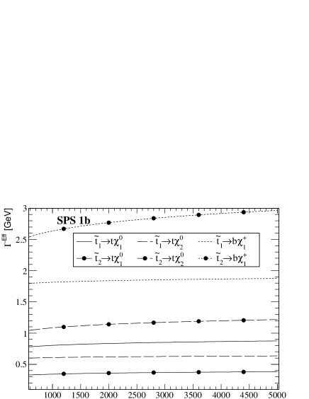
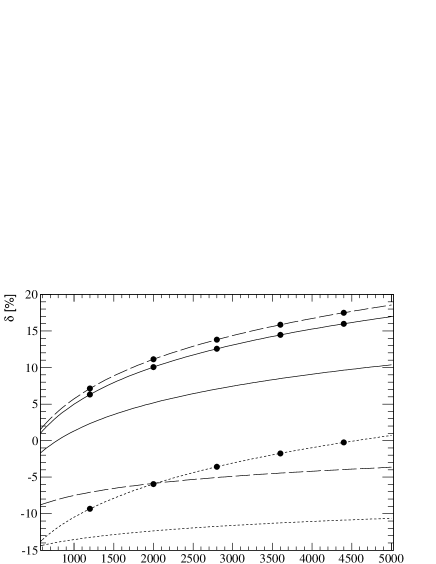
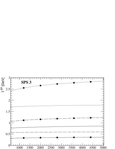
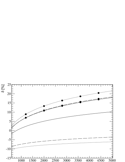
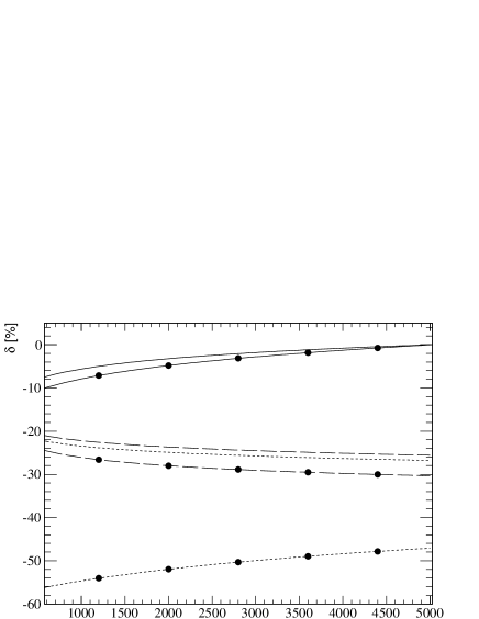
$m_{\tilde{g}}\ [{\rm GeV}]$
(a)	(b)

Figure 1: Effective approximation prediction (Eff) for top-squarks, $\tilde{t}_{1}$ and $\tilde{t}_{2}$, (a) partial decay widths into $\chi_{1}^{0}$ (solid lines), $\chi_{2}^{0}$ (dashed lines) and $\chi_{1}^{+}$ (dotted lines); and (b) relative corrections, $\delta$ eq. (23), in %, as a function of $m_{\tilde{g}}$, for SPS1b (first row), SPS 3 (second row) and SPS 7 (third row) scenarios.

Figures 1 and 2 show the effective approximation prediction for the partial decay widths, $\Gamma$, and relative corrections, $\delta$ (23), of the top-squarks $\tilde{t}_{1}$ and $\tilde{t}_{2}$ decaying into the lightest chargino $(\tilde{t}_{1,2}\rightarrow b\,\chi^{+}_{1})$ and the two lightest neutralinos $(\tilde{t}_{1,2}\rightarrow t\,\chi^{0}_{1,2})$, as a function of $m_{\tilde{g}}$ and $\tan\beta$, respectively. The results are presented for the SPS1b, SPS3 and SPS7 scenarios. In general, one expects the effective approximation to be valid when the gluino mass is much larger than the squark mass scale. We found that the shape of the effective and one-loop approximation can deviate significantly for light gluino masses $400\mbox{\,GeV}<m_{\tilde{g}}<700\mbox{\,GeV}$, and in this case the effective approximation is not appropriate. Since the study presented in this work is only relevant when the gluino is heavy, we can use the effective approximation since it is valid for $m_{\tilde{g}}\gtrsim 900\mbox{\,GeV}$.

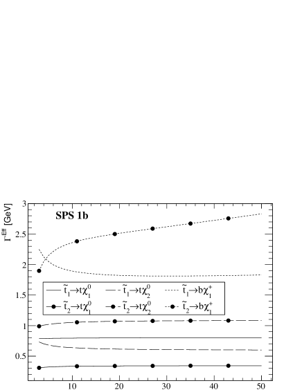
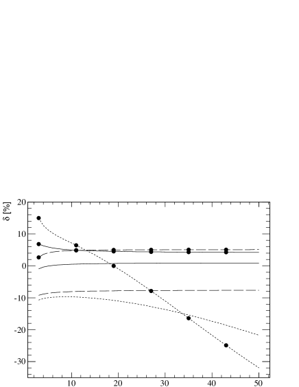
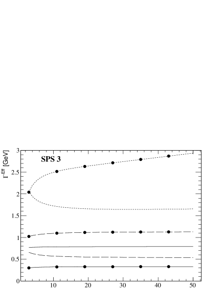
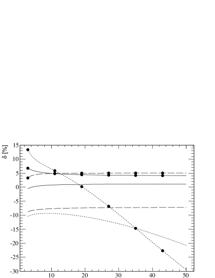
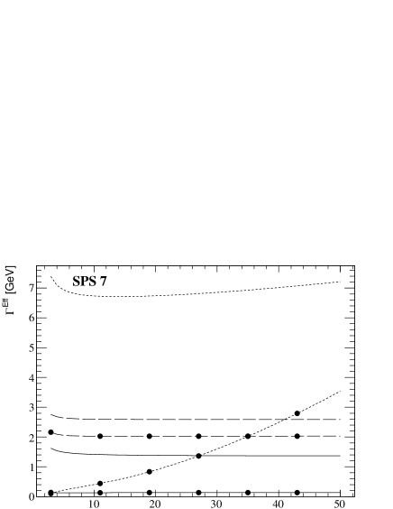
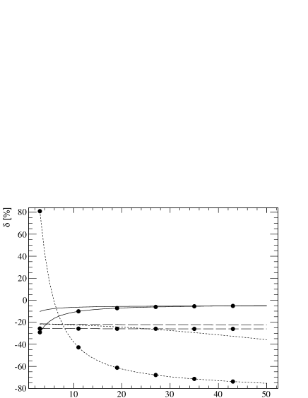
$\tan\beta$
(a)	(b)

Figure 2: Same as Figure 1, but as a function of $\tan\beta$.

Figure 1 shows that, for the SPS1b and SPS3 scenarios, $\Gamma(\tilde{t}_{1}\rightarrow t\chi^{0}_{1})$ has positive corrections for $m_{\tilde{g}}\gtrsim 850\mbox{\,GeV}$. The largest difference with respect to tree-level calculation is obtained at the largest value of the gluino mass $m_{\tilde{g}}=5\mbox{\,TeV}$ ($10\%$). For $\tilde{t}_{1}\rightarrow t\chi^{0}_{2}$ and $\tilde{t}_{1}\rightarrow b\chi^{+}_{1}$ decay channels the corrections are negative and slightly decreasing (in absolute value) with $m_{\tilde{g}}$. Opposite to the SPS1b and SPS3 situation, in the SPS7 scenario, $\chi^{0}_{1,2}$ and $\chi^{+}_{1}$ are mostly of higgsino-type and $\chi^{0}_{3,4}$ and $\chi^{+}_{2}$ are mostly of gaugino-type. Then, the SPS7 scenario has larger partial decay width values into the lightest chargino and neutralinos, and the radiative corrections show a different behaviour. In this scenario all decay channels receive negative corrections in the whole analyzed range of gluino mass. While the (absolute value) corrections in the $\tilde{t}_{1}\rightarrow t\chi^{0}_{1}$ channel decrease with $m_{\tilde{g}}$, the $\tilde{t}_{1}\rightarrow t\chi^{0}_{2}$ and $\tilde{t}_{1}\rightarrow b\chi^{+}_{1}$ channels have an opposite behaviour, becoming more negative as $m_{\tilde{g}}$ increases. For all the SUSY parameter choices, the largest partial decay width values correspond to the decay channel $\tilde{t}_{1}\rightarrow b\chi^{+}_{1}$.

Figure 2 shows the same partial decay widths and relative corrections as before, for SPS1b, SPS3 and for SPS7, as a function of $\tan\beta$. In SPS1b, SPS3 $\tilde{t}_{1}\rightarrow t\chi^{0}_{1}$ receives positive corrections in almost the whole analyzed range of $\tan\beta$, with the exception of the region of small $\tan\beta$ ($\lesssim 6,13$ for SPS1b, SPS3 respectively). For $\tilde{t}_{1}\rightarrow t\chi^{0}_{2},b\chi^{+}_{1}$ decay channels, the radiative corrections are always negative. We found that, for all SPS at $\tan\beta\approx 10$, $\Gamma^{Tree}(\tilde{t}_{1}\rightarrow b\chi^{+}_{1})$ has a minimum and a steep increase for larger $\tan\beta$. The radiative corrections are large and negative, compensating this increase. The one-loop corrections are proportional to $\tan\beta$, and grow faster than the tree-level value, the effective computation, on the other hand, resums the large corrections obtained at large $\tan\beta$, providing a smoother behaviour. For example, in the SPS1b scenario, while $\Gamma^{Tree}(\tilde{t}_{1}\rightarrow b\chi^{+}_{1})$ increases a $25\%$ in the range $\tan\beta=20-50$, the effective prediction $\Gamma^{Eff}(\tilde{t}_{1}\rightarrow b\chi^{+}_{1})$ increases only a $0.4\%$.

For a gluino mass around $\sim 900\mbox{\,GeV}$, corresponding to the nominal value of the chosen SPS, the corrections to $\Gamma(\tilde{t}_{1}\rightarrow t\chi^{0}_{1})$ in SPS1b and SPS3 scenarios are small, below $1\%$ in absolute value in the whole $\tan\beta$ range (see Fig 2b). For SPS7 $\delta$ is larger (in absolute value), evolving from $-9\%$ close to $-5\%$. For the $\chi^{0}_{2}$ decay channel, the deviations $\delta$ are negative: $-10\%<\delta<-7\%$ for SPS1b and SPS3 and $\delta\approx-22\%$ for SPS7. For $\chi^{-}_{1}$ the situation changes, $\delta^{Eff}$ reaches $-36\%$ for SPS7 and $-21\%$ for SPS1b and 3, in absolute values they always increase at a faster rate with $\tan\beta$ if compared to the neutralino channels. We want to stress that neutralino channels show a nearly flat behaviour for $\delta$ because the couplings only involve terms of $\lambda_{t}$ strength ($\propto 1/\tan\beta$), a suppression which wipes out new dependence with $\tan\beta$ introduced by $\Delta m_{t}^{SQCD}$ and log-terms beyond certain $\tan\beta$ ($\approx 10$) for the effective approximation. Meanwhile chargino channels contain terms of $\lambda_{b}$ strength ($\propto\tan\beta$) which enhance higher order corrections. As pointed out above, the SPS7 scenario has the largest radiative corrections. In this scenario, $\chi^{0}_{1}$, $\chi^{0}_{2}$ and $\chi^{+}_{1}$ are of higgsino-type, enhancing higgsino terms ($H_{+}$) in the generic couplings of expression (18). It is clear that large part of the dependence in $\tan\beta$ is encoded in $H_{+}$, and those are also the terms most affected by radiative corrections. SPS1b and SPS3 scenarios have the opposite situation, $\chi^{0}_{1}$, $\chi^{0}_{2}$ and $\chi^{+}_{1}$ are of gaugino-type, therefore gaugino terms ($G$) –depending much less on $\tan\beta$ in the effective approximation– are amplified over $H_{+}$.

For the heavy top-squark ($\tilde{t}_{2}$) decaying into the lightest neutralinos and chargino ($\chi^{0}_{1,2},\chi^{+}_{1}$) as a function of the gluino mass ($m_{\tilde{g}}$) and $\tan\beta$, Fig. 1 shows that the largest partial decay widths correspond to the chargino channel ($\chi^{+}_{1}$) for SPS1b/SPS3 and the second neutralino channel ($\chi^{0}_{2}$) for SPS7. The corrections show the characteristic logarithmic behaviour. For SPS1b/SPS3 the corrections are moderate to large (up to $20\%$) and they are positive, except for the chargino channel in SPS1b. For SPS7 the corrections are negative, they are around $-10\%$ for $\chi^{0}_{1}$, $-30\%$ for $\chi^{0}_{2}$ and $-60\%$ for $\chi^{+}_{1}$. Fig. 2 shows that $\tan\beta$ has its largest impact in the chargino $\chi^{+}_{1}$ channel, both in the partial decay width and in the radiative corrections. We found that the effective approximation moderates the impact of the radiative corrections (see Table 1). While the one-loop corrections may surpass the $-100\%$ value in some cases (e.g. the $\chi^{+}_{1}$ channel in SPS7 for $\tan\beta>41$), meaning that the one-loop correction is not reliable, the effective computation predicts always values that, although quite large, are compatible with perturbation theory (e.g. $-75\%$ in that case), and we can rely on this computation.

Decay	SPS1b			SPS3
	$\Gamma^{Tree}$	$\delta^{Eff}$	$\delta^{1-loop}$	$\Gamma^{Tree}$	$\delta^{Eff}$	$\delta^{1-loop}$
$\tilde{t}_{1}\rightarrow t\chi^{0}_{1}$	0.7927	0.8	0.2	0.7769	0.8	0.2
$\tilde{t}_{1}\rightarrow t\chi^{0}_{2}$	0.6577	-7.7	-7.3	0.6193	-7.7	-7.2
$\tilde{t}_{1}\rightarrow t\chi^{0}_{3}$	-	-	-	-	-	-
$\tilde{t}_{1}\rightarrow t\chi^{0}_{4}$	-	-	-	-	-	-
$\tilde{t}_{1}\rightarrow b\chi^{+}_{1}$	2.099	-13.7	-18.0	1.903	-9.4	-11.5
$\tilde{t}_{1}\rightarrow b\chi^{+}_{2}$	0.9378	-39.9	-47.8	0.4941	-30.9	-31.9
$\tilde{t}_{2}\rightarrow t\chi^{0}_{1}$	0.3262	4.4	3.7	0.3075	4.9	4.2
$\tilde{t}_{2}\rightarrow t\chi^{0}_{2}$	1.026	5.1	4.4	1.043	4.9	4.3
$\tilde{t}_{2}\rightarrow t\chi^{0}_{3}$	1.489	-29.0	-28.7	1.362	-29.0	-28.5
$\tilde{t}_{2}\rightarrow t\chi^{0}_{4}$	3.764	-25.6	-27.6	3.509	-25.7	-27.6
$\tilde{t}_{2}\rightarrow b\chi^{+}_{1}$	2.946	-11.0	-21.5	2.343	6.5	3.6
$\tilde{t}_{2}\rightarrow b\chi^{+}_{2}$	4.900	-51.7	-73.1	2.472	-28.8	-33.8
	SPS7			Def $\,\,m_{\tilde{g}}=1\mbox{\,TeV}$			Def $\,\,m_{\tilde{g}}=3\mbox{\,TeV}$
	$\Gamma^{Tree}$	$\delta^{Eff}$	$\delta^{1-loop}$	$\Gamma^{Tree}$	$\delta^{Eff}$	$\delta^{1-loop}$	$\delta^{Eff}$	$\delta^{1-loop}$
$\tilde{t}_{1}\rightarrow t\chi^{0}_{1}$	1.481	-5.9	-6.5	0.1264	11.5	7.8	22.9	15.2
$\tilde{t}_{1}\rightarrow t\chi^{0}_{2}$	3.323	-22.0	-22.1	1.174	-2.1	-3.2	3.6	1.9
$\tilde{t}_{1}\rightarrow t\chi^{0}_{3}$	5.776	-27.5	-28.4	2.963	-29.1	-24.8	-33.9	-27.5
$\tilde{t}_{1}\rightarrow t\chi^{0}_{4}$	0.5845	-40.2	-40.2	5.298	-23.7	-20.9	-26.7	-22.4
$\tilde{t}_{1}\rightarrow b\chi^{+}_{1}$	8.754	-23.3	-25.4	1.642	16.1	10.1	29.4	20.2
$\tilde{t}_{1}\rightarrow b\chi^{+}_{2}$	1.493	-43.4	-47.3	3.737	-20.5	-19.3	-22.0	-19.7
$\tilde{t}_{2}\rightarrow t\chi^{0}_{1}$	0.1435	-8.2	-13.1	2.103	-5.5	-8.7	-1.2	-1.4
$\tilde{t}_{2}\rightarrow t\chi^{0}_{2}$	2.730	-25.9	-27.6	3.299	-16.9	-17.6	-16.7	-14.1
$\tilde{t}_{2}\rightarrow t\chi^{0}_{3}$	4.723	-29.4	-30.2	9.944	-29.2	-28.2	-33.1	-29.2
$\tilde{t}_{2}\rightarrow t\chi^{0}_{4}$	5.624	-19.0	-20.5	4.515	-34.7	-31.9	-40.4	-35.2
$\tilde{t}_{2}\rightarrow b\chi^{+}_{1}$	1.371	-54.9	-69.6	7.531	-16.9	-18.6	-16.8	-15.0
$\tilde{t}_{2}\rightarrow b\chi^{+}_{2}$	6.262	-16.7	-19.6	8.662	-34.5	-33.4	-40.0	-36.5

Table 1: Tree-level decay width, $\Gamma^{Tree}$ [GeV], and relative radiative corrections, $\delta^{Eff}$ and $\delta^{1-loop}$ $[\%]$ (23), for the various SPS scenarios and Def (with two values of $m_{\tilde{g}}=1,\,3\mbox{\,TeV}$).

Finally, Table 1 summarizes the results for the tree-level computation, $\Gamma^{Tree}$ [GeV], and the relative radiative corrections, $\delta^{Eff}$ $[\%]$ and $\delta^{1-loop}$ (23), of all surveyed partial decay widths. Numbers not shown correspond to kinematically closed channels. The results are shown for the three SPS scenarios analyzed in this paper SPS1b, SPS3, SPS7, and Def, eq. (20). We include two sets of Def parameters: one with $m_{\tilde{g}}=3\mbox{\,TeV}$ as in eq. (20), and one with $m_{\tilde{g}}=1\mbox{\,TeV}$. The reason is a fair comparison among the various SUSY scenarios: since the radiative corrections grow as the logarithm of $m_{\tilde{g}}$, the corrections in the Def parameter set are enhanced over those of the SPS, which have a $m_{\tilde{g}}\simeq 1\mbox{\,TeV}$. A quick look at Table 1 shows that the radiative corrections are quite different in each channel, which means that they will have an impact on the decay branching ratios (and production cross-sections). As an example, in SPS1b the tree-level prediction is that the largest branching ratio of the heavy top-squark corresponds to the second chargino ($\tilde{t}_{2}\to b\chi^{+}_{2}$), followed by $\chi^{0}_{4}$ and $\chi^{+}_{1}$, however, after computing the radiative corrections one finds that the largest branching ratio corresponds to $\Gamma(\tilde{t}_{2}\to t\chi^{0}_{4})\simeq 2.8\mbox{\,GeV}$, followed by $\Gamma(\tilde{t}_{2}\to b\chi^{+}_{1})\simeq 2.6\mbox{\,GeV}$, and $\Gamma(\tilde{t}_{2}\to b\chi^{+}_{2})\simeq 2.4\mbox{\,GeV}$ in third place.

5.3 Cross-Section Computation

After successfully implementing and checking our effective MSSM couplings in MadGraph, we have computed the cross-section of top-squark pair production for the Def, SPS1b, SPS3 and SPS7 scenarios. We have focussed on reactions where top-squarks decay into the two lightest neutralinos ($\chi^{0}_{1,2}$) and the lightest chargino ($\chi^{\pm}_{1}$), since these are the search channels used at the LHC [3, 4, 11]. The ATLAS collaboration has already used them to analyze LHC data and set limits on top-squark pair-production [19, 20, 21, 24, 25].

We have simulated proton-proton ($pp$) collisions at $14\mbox{\,TeV}$ using the CTEQ6L set of parton distribution functions. Our aim is to use the standard MadGraph input files as far as possible. By default, MadGraph sets renormalization and factorization scales dynamically. For the production of a pair of heavy particles, as is our case, these scales are set equal to the geometric mean of $M^{2}+p_{T}^{2}$ of both particles, where $M$ is the mass of the particle and $p_{T}$ is its transverse momentum. The scale $Q$ of the effective couplings (19) is fixed at the mass of the internal top-squark for each process.

In this section we present the results for the top-squark pair production cross-section in $pp$ collisions, followed by the decay into a quark and charginos and neutralinos, including the effect of the radiative corrections in the effective coupling approximation.

5.3.1 $\sigma(pp\rightarrow({q}^{{}^{\prime}}{\chi}_{r})({\bar{q}}^{{}^{\prime\prime}}\chi_{s}))$

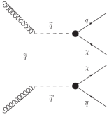
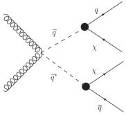
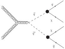
(a)	(b)	(c)
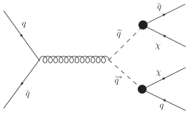
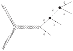
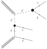
(d)	(e)	(f)
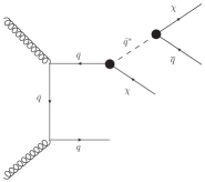
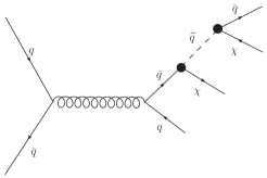
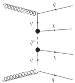
(g)	(h)	(i)

Figure 3: Generic partonic Feynman diagrams contributing to $\sigma(pp\rightarrow({q}\chi)({\bar{q}}\chi))$, (a)-(d) double resonant diagrams ($\sigma(pp\to\tilde{q}_{a}\tilde{q}_{a}^{*}\rightarrow({q}\chi)({\bar{q}}\chi))$), (e)-(h) single resonant diagrams, (i) non-resonant diagram.

The cross-section we consider in this work is

$$\sigma\left(pp(\to[\tilde{q}_{a},\tilde{q}_{a}\tilde{q}_{a}^{*}])\rightarrow({q}^{{}^{\prime}}\chi_{r})({\bar{q}}^{{}^{\prime\prime}}\chi_{s})\right)\ \ ,\ \ \tilde{q}_{a}=\tilde{t}_{1,2}\ ,\ \ {q}^{{}^{\prime}},{\bar{q}}^{{}^{\prime\prime}}=t,b\ ,\ \ \chi_{r,s}=\chi^{\pm}_{1},\chi^{0}_{1,2}\ ,$$ (24)

that is: chargino or neutralino production, associated with top and bottom quarks, which proceeds through a single or double top-squark in the intermediate states. Figure 3 shows the partonic Feynman diagrams. Figs. 3a-d show the double-resonant diagrams contributing to the process we are interested in: $\sigma(pp\to\tilde{q}_{a}\tilde{q}_{a}^{*}\rightarrow({q}\chi)({\bar{q}}\chi))$, however, this set of diagrams is not gauge invariant. The complete set of gauge-invariant diagrams includes also single-resonant diagrams (Fig. 3e-h) and non-resonant diagrams (Fig. 3i). We have checked that quark-anti-quark channels ($q\bar{q}$, Fig. 3d,h) are three times smaller than the gluon-gluon channel ($gg$), i.e. they represent less than a $30\%$ of the total cross-section. Both channels are included in our computation. Since all top-squarks contribute to the same final state, one should add up all the amplitudes in Fig. 3 for $\tilde{t}_{1}$ and $\tilde{t}_{2}$, however in squark search studies it is costumary to separate the $\tilde{t}_{1}$ and $\tilde{t}_{2}$ channels, and look for each signal separately. For this reason we will show results for the cross-section with only one of the top-squarks in the intermediate states of Fig. 3. This separation is possible because we have checked that the interference effects between $\tilde{t}_{1}$ and $\tilde{t}_{2}$ channels is less than $0.8\%$. We will denote this process as:

$$pp\to[\tilde{q}_{a}]\to X$$

where $\tilde{q}_{a}$ is the squark appearing in the intermediate state, and $X$ is the final state, under the understanding that all diagrams (double-resonant, single-resonant, and non-resonant) contribute.

Before performing the full simulation it is useful to analyze approximations to the quantity under study. Under the narrow width approximation the total cross-section (24) can be computed as the squark pair production cross-section followed by the decay branching ratios,

$$\sigma\left(pp\rightarrow[\tilde{q}_{a}]\rightarrow({q}^{{}^{\prime}}\chi_{r})({\bar{q}}^{{}^{\prime\prime}}\chi_{s})\right)\simeq\sigma(pp\rightarrow\tilde{q}_{a}\tilde{q}_{a}^{\ast})\times BR(\tilde{q}_{a}\rightarrow{q}^{{}^{\prime}}\chi_{r})\times BR(\tilde{q}_{a}^{\ast}\rightarrow{\bar{q}}^{{}^{\prime\prime}}\chi_{s})\,.$$ (25)

In this approximation only the double-pole diagrams (Fig. 3a-d) contribute. In the present process the first part $\sigma(pp\rightarrow\tilde{q}_{i}\tilde{q}_{i}^{\ast})$ proceeds purely through standard QCD couplings, the only SUSY parameters being the squark masses. All the information on SUSY couplings is in the second part of the expression, that is, in the decay branching ratios or partial decay widths, which have been analyzed in section 5.2. The top-squark production cross-section has been computed to NLO-SUSY-QCD [79] and NLL-SUSY-QCD [80], the radiative corrections increase the production cross-section at the $14\mbox{\,TeV}$ LHC by a $25\%-50\%$ depending on the top-squark mass, with a mild dependence on other SUSY parameters [79, 80].

In order to asses the effects of the radiative corrections, it is useful to define a factor $K_{SUSY}$ as:

$$K_{SUSY}=\frac{\sigma_{Effective}}{\sigma_{Tree}}\ \ ,$$ (26)

which under the narrow-width approximation of eq. (25) can be computed as a ratio of partial decay widths:

$$K_{SUSY} = \frac{K_{partial}}{K_{full}}$$

$$K_{partial} = \frac{\Gamma^{Eff}(\tilde{q}\rightarrow{q}^{{}^{\prime}}\chi_{r})}{\Gamma^{Tree}(\tilde{q}\rightarrow{q}^{{}^{\prime}}\chi_{r})}\times\frac{\Gamma^{Eff}(\tilde{q}^{\ast}\rightarrow{\bar{q}}^{{}^{\prime\prime}}\chi_{s})}{\Gamma^{Tree}(\tilde{q}^{\ast}\rightarrow{\bar{q}}^{{}^{\prime\prime}}\chi_{s})}$$

$$K_{full} = \left(\frac{\Gamma^{Eff}_{full}}{\Gamma^{Tree}_{full}}\right)^{2}$$ (27)

where $\Gamma_{full}$ is the full decay width and Eff and Tree stand for the effective approximation and the tree-level computation. For the parameter space points of the present study, all bosonic $\tilde{t}_{1}$ decay channels are kinematically closed, and therefore the full decay width consists only of the chargino/neutralino (inos) channels. Bosonic channels have some impact on the $\tilde{t}_{2}$ full decay width. $K_{SUSY}$ is composed of two factors: $K_{partial}$, regarding the partial decay widths of the produced squarks decaying into a quark and the selected final particles ($\chi^{0}_{1,2}$ or $\chi^{\pm}_{1}$ analyzed in section 5.2) and $K_{full}$ the radiative correction to the total decay width. For the parameter space explored in the present work we have found that the radiative corrections to the total decay width are always negative ($K_{full}<1$). Of course, using the narrow-width approximation (25) one can not compute angular distributions or correlations, something that it is possible to perform with the MadGraph implementation.

The results for the cross-sections are summarized in Figures 4-9, where we show the tree-level and effective approximation cross-section computations, as well as the $K_{SUSY}$ (26) factor, as a function of $\tan\beta$ and $m_{\tilde{g}}$.

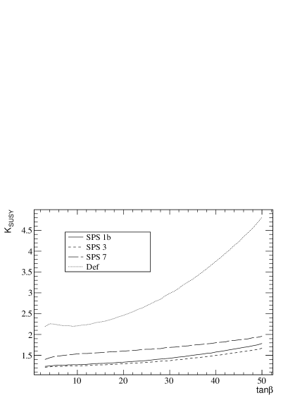
(a)	(b)

Figure 4: (a) Cross-section of $pp\rightarrow[\tilde{t}_{1}]\rightarrow t\chi^{0}_{1}\bar{t}\chi^{0}_{1}$ and (b) $K_{SUSY}$, as a function of $\tan\beta$ and $m_{\tilde{g}}$ for the input parameters as defined in SPS1b, 3, 7 and Def (20).

Figures 4-6 present the cross-section corresponding to the lightest top-squark $\tilde{t}_{1}$. Fig. 4a shows the results for $\sigma(pp\rightarrow[\tilde{t}_{1}]\rightarrow(t\chi^{0}_{1})(\bar{t}\chi^{0}_{1}))$ as a function of $m_{\tilde{g}}$ and $\tan\beta$ for the different scenarios of the SUSY input parameters analyzed in this work. The ratio $K_{SUSY}$ is shown in Fig. 4b. The radiative corrections are positive in all scenarios, this is due to the combination of two factors: first, the radiative corrections to the partial decay width $\Gamma(\tilde{t}_{1}\to b\chi^{0}_{1})$ are positive in the scenarios SPS1b, SPS3 and Def (Figs. 1, 2 and Table 1), providing a $K_{partial}>1$, but, more importantly, the radiative corrections to the total decay width are negative, providing a $K_{full}<1$, and therefore a $K_{SUSY}>1$ (see eq. (27)), as can be seen in Table 1. For example, in SPS1b the leading decay channels (at the tree-level) are $b\chi^{+}_{1}$ and $b\chi^{+}_{2}$, but they have negative radiative corrections of $-13.7\%$ and $-39.9\%$ respectively, in the end, when taking into account all channels one obtains $\Gamma_{full}^{Tree}=4.49\mbox{\,GeV}$, $\Gamma_{full}^{Eff}=3.78\mbox{\,GeV}$, providing $K_{full}=(0.84)^{2}\simeq 0.71\simeq 1/1.41$, so a $\delta_{full}^{Eff}=-26\%$ radiative correction to the total decay width translates to a $41\%$ enhancement of the production cross-section. The increase of the radiative corrections $K_{SUSY}$ with $m_{\tilde{g}}$ is given by the $\log(m_{\tilde{g}})$-terms (19) of the effective computation. This figure shows the importance of the radiative corrections, which can enhance the cross-section by a large factor (between $1.2$ and $5$ in Fig. 4), and also of the newly included $\log(m_{\tilde{g}})$-terms, the log terms produce an increase of the $K_{SUSY}$-factor (and hence the cross-section) of $1.6/1.4=1.14$, $1.4/1.2=1.17$, $2/1.5=1.33$, $2.4/1.7=1.41$ in the range $m_{\tilde{g}}=1000-5000\mbox{\,GeV}$ for the scenarios SPS1b, SPS3, SPS7, Def respectively. The largest cross-sections are obtained in the SPS1b and SPS3 scenarios, which have a similar behaviour of the corrections. At $\tan\beta=30$, the cross-section values in the effective approximation are $4.08\times 10^{-3}$ pb (SPS1b) and $5.38\times 10^{-3}$ pb (SPS3), a factor $1.43$ and $1.37$ larger than the tree-level prediction respectively. The SPS7 scenario provides an intermediate value of the cross-section in our analysis. For $\tan\beta=15$ and $m_{\tilde{g}}=926\mbox{\,GeV}$ (as fixed in this scenario) the effective prediction for the cross-section is $1.82\times 10^{-4}$ pb, a factor $1.56$ larger than the tree-level prediction (see Fig. 4b). The tree-level cross-sections decrease as a function of $\tan\beta$ in the region $\tan\beta>10$, this behaviour is softened by the positive radiative corrections. We recall that the squark masses (and hence phase-space factors) also change with $\tan\beta$, i.e. $m_{\tilde{t}_{1}}$ changes from $772\mbox{\,GeV}$ to $780\mbox{\,GeV}$. The smaller values of the cross-section are obtained in the Def scenario (20), e.g. $\sigma^{Eff}=6.54\times 10^{-6}$ pb for the effective computation prediction at $\tan\beta=5$, a factor $2.25$ larger than the tree-level prediction. The largest radiative corrections are obtained at large $\tan\beta$, with $K_{SUSY}=4.81$. We recall that in this scenario $m_{\tilde{g}}=3\mbox{\,TeV}$, enhancing the radiative corrections.

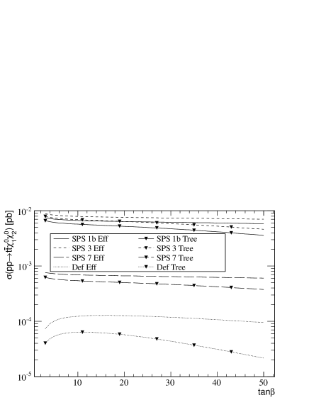
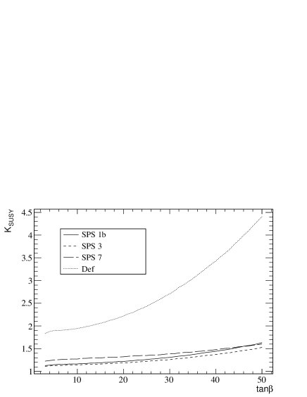
(a)	(b)

Figure 5: (a) Cross-section of $pp\rightarrow[\tilde{t}_{1}]\rightarrow t\chi^{0}_{2}\bar{t}\chi^{0}_{1}$ and (b) $K_{SUSY}$, as a function of $\tan\beta$ and $m_{\tilde{g}}$ for the input parameters as defined in SPS1b, 3, 7 and Def (20).

The results for $\sigma(pp\rightarrow[\tilde{t}_{1}]\rightarrow t\chi^{0}_{2}\bar{t}\chi^{0}_{1})$ are presented in Fig. 5. For SPS1b/SPS3 the cross-sections are slightly larger than the $(t\chi^{0}_{1})(t\chi^{0}_{1})$ channel (Fig. 4), whereas they are much larger for SPS7/Def. We can trace back this behaviour to the relative value of the partial decay widths (Figs. 1, 2, Table 1) and combinatorial factors. First of all, there is a factor $2$ combinatorial enhancement factor because now the particles in the final state are different. Then in SPS1b/SPS3 there is a slight suppression because $BR(\tilde{t}_{1}\to t\chi^{0}_{2})<BR(\tilde{t}_{1}\to t\chi^{0}_{1})$, whereas in SPS7/Def there is a large enhancement because $BR(\tilde{t}_{1}\to t\chi^{0}_{2})\gg BR(\tilde{t}_{1}\to t\chi^{0}_{1})$. The radiative corrections (Fig. 5b) are smaller than in the $(t\chi^{0}_{1})(t\chi^{0}_{1})$ channel (Fig. 4b), this is due to the fact that the radiative corrections are smaller (more negative) for the partial decay width $\Gamma(\tilde{t}_{1}\to t\chi^{0}_{2})$ than for $\Gamma(\tilde{t}_{1}\to t\chi^{0}_{1})$ (Table 1). This channel in the Def scenario has a cross-section one order of magnitude larger than the $(t\chi^{0}_{1})(t\chi^{0}_{1})$ channel.

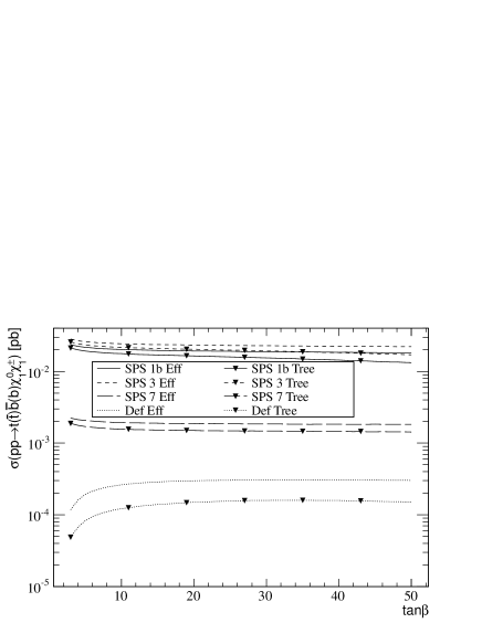
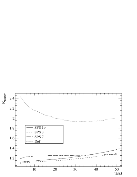
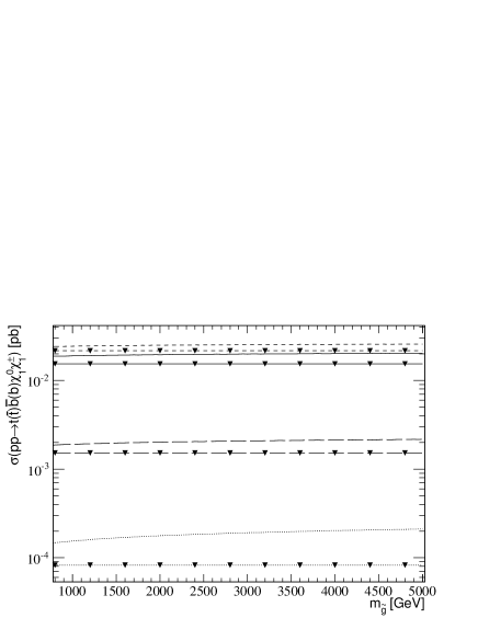
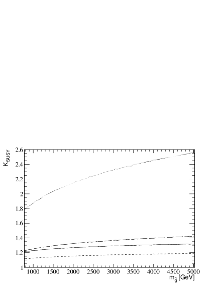
(a)	(b)

Figure 6: (a) Cross-section $\sigma(pp\rightarrow[\tilde{t}_{1}]\rightarrow b\chi^{+}_{1}\bar{t}\chi^{0}_{1})+\sigma(pp\to[\tilde{t}_{1}]\to\bar{b}\chi^{-}_{1}t\chi^{0}_{1})$ and (b) $K_{SUSY}$, as a function of $\tan\beta$ and $m_{\tilde{g}}$ for the input parameters as defined in SPS1b, 3, 7 and Def (20).

To finish with the $\tilde{t}_{1}$ production analysis, Fig. 6 shows the cross-sections and radiative corrections for the lightest neutralino ($\chi^{0}_{1}$) and chargino ($\chi^{\pm}_{1}$) production mediated by $\tilde{t}_{1}$. Since the experimental analysis does not perform charge identification, both charge-conjugate channels $\sigma(pp\rightarrow[\tilde{t}_{1}]\to t\chi^{0}_{1}\bar{b}\chi^{-}_{1})$ and $\sigma(pp\rightarrow[\tilde{t}_{1}]\to\bar{t}\chi^{0}_{1}b\chi^{+}_{1})$ contribute to the same experimental signal, therefore Fig. 6a shows the sum of both cross-sections. This channel provides the largest cross-section for $\tilde{t}_{1}$-pair production in all studied scenarios. For example, at $\tan\beta=30$, the cross-section values in the effective approximation are $1.89\times 10^{-2}$ pb (SPS1b), $2.29\times 10^{-2}$ pb (SPS3), $1.85\times 10^{-3}$ pb (SPS7) and $3.08\times 10^{-4}$ pb (Def). The radiative corrections (Fig. 6b) are slightly smaller in this channel for the SPS scenarios, providing $K_{SUSY}$ factors in the range $K_{SUSY}\simeq 1.1-1.4$ ($10\%-40\%$ increase of the cross-section). The Def scenario has the largest radiative corrections for the reference value $\tan\beta=5$ (20), but they have a different behaviour than the previous channels (Figs. 4, 5) at large $\tan\beta$: they decrease instead of growing at large $\tan\beta$. In this scenario the leading $\tilde{t}_{1}$ decay channels are $\chi^{0}_{3,4}$ and $\chi^{+}_{2}$, all of them having negative corrections (Table 1) which grow with $\tan\beta$. This provides a growing contribution to $K_{SUSY}$ through $1/K_{full}$ (27). The other contribution, $K_{partial}$, has two distinct factors: the radiative corrections to $\Gamma(\tilde{t}_{1}\to t\chi^{0}_{1})$ have a nearly flat behaviour with $\tan\beta$ at a value around $18\%-22\%$, but the radiative corrections to $\Gamma(\tilde{t}_{1}\to b\chi^{+}_{1})$ have a strong decreasing behaviour from $\sim 29\%$ ($\tan\beta=5$) to $\sim-52\%$ ($\tan\beta=50$). This decrease in $K_{partial}$ partially compensates for the increase due to $1/K_{full}$ resulting in a more flat behaviour with $\tan\beta$ as compared with the $t\chi^{0}_{\alpha}\bar{t}\chi^{0}_{\beta}$ channels.

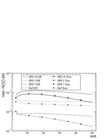
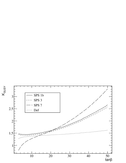
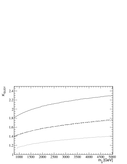
(a)	(b)

Figure 7: (a) Cross-section of $pp\rightarrow[\tilde{t}_{2}]\rightarrow t\chi^{0}_{1}\bar{t}\chi^{0}_{1}$ and (b) $K_{SUSY}$, as a function of $\tan\beta$ and $m_{\tilde{g}}$ for the input parameters as defined in SPS1b, 3, 7 and Def (20).

The results for the $\tilde{t}_{2}$ mediated cross-sections are shown in figures 7-9. The values of these cross-sections are smaller than for the $\tilde{t}_{1}$ mediated cross-sections. Fig. 7 presents the cross-section $\sigma(pp\rightarrow[\tilde{t}_{2}]\rightarrow t\chi^{0}_{1}\bar{t}\chi^{0}_{1})$ and the corresponding radiative corrections. Radiative corrections are positive (except for a small corner at low $\tan\beta$ for SPS7), enhancing the cross-section, which stays in the $10^{-7}-10^{-5}$ pb range. The largest results for the cross-section are obtained in the SPS1b and SPS3 scenarios, which have similar values, and they overlap in the plots as function of $\tan\beta$. At $\tan\beta=30$, the corresponding values in the effective approximation are $1.094\times 10^{-5}$ pb (SPS1b) and $1.098\times 10^{-5}$ pb (SPS3). The different results between these points (when plotted as a function of $m_{\tilde{g}}$) arise from the different nominal values of $\tan\beta$ (see appendix A). The same similarities occur in the other channels (Figs. 8, 9), but not as pronounced as the present one. In scenario Def we obtain an intermediate value of the cross-section ($3.37\times 10^{-6}$ pb), and the lowest value is obtained in the SPS7 scenario ($7.29\times 10^{-7}$ pb). Note the quite distinct behaviour of the radiative corrections (Fig. 7b) as compared with the $\tilde{t}_{1}$ channels (Fig. 4b): in the present channel the Def scenario has smaller radiative corrections, and a flatter evolution with $\tan\beta$. Quite opposite, the SPS scenarios have larger radiative corrections and a steeper slope as a function of $\tan\beta$. The radiative corrections tend to soften the slopes of the cross-sections as a function of $\tan\beta$. We note also a small region of negative radiative corrections for SPS7 at low $\tan\beta<7$.

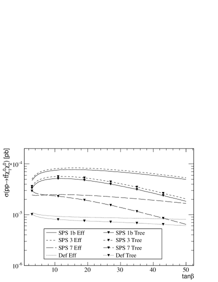
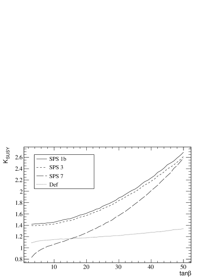
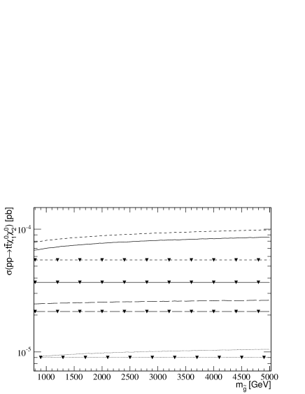
(a)	(b)

Figure 8: (a) Cross-section of $pp\rightarrow[\tilde{t}_{2}]\rightarrow t\chi^{0}_{2}\bar{t}\chi^{0}_{1}$ and (b) $K_{SUSY}$, as a function of $\tan\beta$ and $m_{\tilde{g}}$ for the input parameters as defined in SPS1b, 3, 7 and Def (20).

Figure 8 shows the results for $\sigma(pp\rightarrow[\tilde{t}_{2}]\rightarrow t\chi^{0}_{2}\bar{t}\chi^{0}_{1})$. The cross-sections are larger than in the $\chi^{0}_{1}\chi^{0}_{1}$ channel in all scenarios, being in the range of $10^{-6}-10^{-5}$ pb. The largest values are again obtained for the SPS1b and SPS3 scenarios. In these two scenarios, the partial decay widths of $\tilde{t}_{2}$ decaying into $\chi^{0}_{1,2}$ have always positive radiative corrections in the whole explored region of gluino masses and $\tan\beta$ (Figs. 1b, 2b), providing an enhancement to $K_{SUSY}$, additional to the negative correction to the total decay width ($K_{full}<1$). The cross-sections for SPS7 and Def have a mild evolution with $\tan\beta$, and the radiative corrections are smaller than in the $\chi^{0}_{1}\chi^{0}_{1}$ channel.

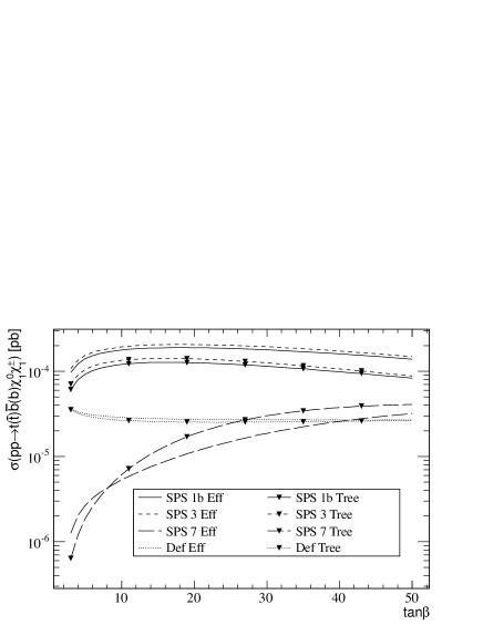
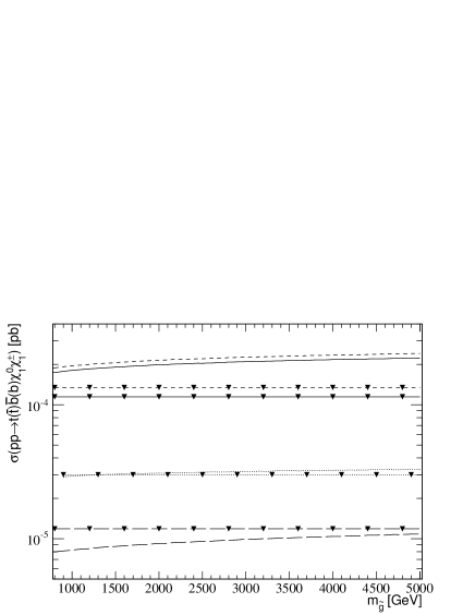
(a)	(b)

Figure 9: (a) Cross-section $\sigma(pp\rightarrow[\tilde{t}_{2}]\to b\chi^{+}_{1}\bar{t}\chi^{0}_{1})+\sigma(pp\to[\tilde{t}_{2}]\to\bar{b}\chi^{-}_{1}t\chi^{0}_{1})$ and (b) $K_{SUSY}$, as a function of $\tan\beta$ and $m_{\tilde{g}}$ for the input parameters as defined in SPS1b, 3, 7 and Def (20).

Finally, we present the results for the chargino-neutralino channel in Fig. 9. Again, the plots in Fig. 9 contain the sum of the two charge-conjugate modes: $\sigma(pp\rightarrow[\tilde{t}_{2}]\to b\chi^{+}_{1}\bar{t}\chi^{0}_{1})+\sigma(pp\to[\tilde{t}_{2}]\to\bar{b}\chi^{-}_{1}t\chi^{0}_{1})$. This channel provides the largest cross-section for $\tilde{t}_{2}$ production in the SPS1b, SPS3 and Def scenarios. In these scenarios the radiative corrections are smaller than previous channels, and they have a quite flat evolution with $\tan\beta$ and $m_{\tilde{g}}$. In contrast, in the SPS7 scenario we find a steep evolution with $\tan\beta$ of both: the cross-section and the radiative corrections. This evolution is inherited from the partial decay width $\Gamma(\tilde{t}_{2}\to b\chi^{+}_{1})$ (Fig. 2). The radiative corrections are negative in a wide region of parameters, producing a decrease of the cross-section.

Let us note that the main $\tilde{t}_{2}$ decay channels correspond to $\chi^{0}_{3,4}$ in the neutralino sector and $\chi^{+}_{2}$ in the chargino sector (Table 1), together these channels are responsible for more than $60\%$ of the $\tilde{t}_{2}$ decay branching ratio in all studied scenarios. At the same time, these leading channels have large negative radiative corrections ($|\delta^{Eff}|>20\%$), providing a large $1/K_{full}$ (27). For the SPS1b, SPS3, Def scenarios the radiative corrections to $\Gamma(\tilde{t}_{2}\to b\chi^{+}_{1})$ are quite moderate and negative (Figs. 1, 2, Table 1) producing a small reduction of $K_{SUSY}$ through $K_{partial}$. But for SPS7 the radiative corrections are larger, and have a very strong $\tan\beta$ dependence $\delta^{Eff}\simeq(80\%,40\%,-75\%)$ for $\tan\beta=(2,5,50)$ (Fig. 2), for $\tan\beta\gtrsim 10$ the negative corrections to $\Gamma(\tilde{t}_{2}\to b\chi^{+}_{1})$ (negative contribution to $K_{SUSY}$) overcompensate the negative corrections to the total decay width $\Gamma_{full}$ (positive contribution to $K_{SUSY}$), providing an overall negative contribution to the cross-section radiative corrections.

To complete the discussion in this section, Table 2 shows the radiative correction factor $K_{SUSY}$ (26) for all the production channels cross-sections and all the scenarios presented in this work. Results are shown for three different values of $\tan\beta$, to make the comparison more meaningful. For the same reason the Def scenario is shown also for a light gluino mass $m_{\tilde{g}}=1\mbox{\,TeV}$. In general, the radiative corrections are positive, increasing the production cross-section. As analyzed above, this is mainly (but not only) due to the fact that the radiative corrections decrease the top-squark total decay width. For $m_{\tilde{g}}=1\mbox{\,TeV}$ the positive corrections provide a $K_{SUSY}$ factor between $1.05$ and $3.91$, depending on the channel and scenario. Negative radiative corrections are only obtained for $\sigma(pp\rightarrow[\tilde{t}_{2}]\rightarrow(b\chi^{+}_{1})(\bar{t}\chi^{0}_{1}))$ in the SPS7 scenario and the Def scenario at $m_{\tilde{g}}=1\mbox{\,TeV}$, due to large negative corrections to $\Gamma(\tilde{t}_{2}\to b\chi^{+}_{1})$ (Fig. 2 and Table 1), they provide a $K_{SUSY}$ between $0.62$ and $0.99$ depending on the scenario. The largest radiative corrections are obtained at large $\tan\beta$. We recall that the corrections grow with the gluino mass (e.g. $K_{SUSY}=4.81$ for $\tan\beta=50$, $m_{\tilde{g}}=3\mbox{\,TeV}$ in the $(\chi^{0}_{1}\chi^{0}_{1})$ channel and Def scenario).

$K_{SUSY}$	SPS7			Def
	$m_{\tilde{g}}=926.0\mbox{\,GeV}$			$m_{\tilde{g}}=1\mbox{\,TeV}$			$m_{\tilde{g}}=3\mbox{\,TeV}$
$\tan\beta$	10	30	50	10	30	50	10	30	50
$pp\rightarrow[\tilde{t}_{1}]\rightarrow(t\chi^{0}_{1})(\bar{t}\chi^{0}_{1})$	1.53	1.69	1.95	1.83	2.46	3.91	2.20	2.98	4.81
$pp\rightarrow[\tilde{t}_{1}]\rightarrow(t\chi^{0}_{2})(\bar{t}\chi^{0}_{1})$	1.27	1.38	1.60	1.66	2.32	3.71	1.94	2.70	4.40
$pp\rightarrow[\tilde{t}_{1}]\rightarrow(b\chi^{+}_{1})(\bar{t}\chi^{0}_{1})$	1.24	1.25	1.27	1.77	1.62	1.62	2.15	1.93	2.00
$pp\rightarrow[\tilde{t}_{2}]\rightarrow(t\chi^{0}_{1})(\bar{t}\chi^{0}_{1})$	1.28	2.00	3.31	1.20	1.28	1.40	1.37	1.47	1.62
$pp\rightarrow[\tilde{t}_{2}]\rightarrow(t\chi^{0}_{2})(\bar{t}\chi^{0}_{1})$	1.06	1.57	2.59	1.05	1.11	1.22	1.15	1.22	1.34
$pp\rightarrow[\tilde{t}_{2}]\rightarrow(b\chi^{+}_{1})(\bar{t}\chi^{0}_{1})$	0.87	0.62	0.78	0.99	0.98	0.93	1.08	1.06	1.01
	SPS1b			SPS3
	$m_{\tilde{g}}=916.1\mbox{\,GeV}$			$m_{\tilde{g}}=914.3\mbox{\,GeV}$
$\tan\beta$	10	30	50	10	30	50
$pp\rightarrow[\tilde{t}_{1}]\rightarrow(t\chi^{0}_{1})(\bar{t}\chi^{0}_{1})$	1.27	1.42	1.78	1.24	1.37	1.66
$pp\rightarrow[\tilde{t}_{1}]\rightarrow(t\chi^{0}_{2})(\bar{t}\chi^{0}_{1})$	1.16	1.30	1.63	1.13	1.25	1.52
$pp\rightarrow[\tilde{t}_{1}]\rightarrow(b\chi^{+}_{1})(\bar{t}\chi^{0}_{1})$	1.14	1.22	1.37	1.11	1.18	1.29
$pp\rightarrow[\tilde{t}_{2}]\rightarrow(t\chi^{0}_{1})(\bar{t}\chi^{0}_{1})$	1.46	1.86	2.66	1.42	1.81	2.58
$pp\rightarrow[\tilde{t}_{2}]\rightarrow(t\chi^{0}_{2})(\bar{t}\chi^{0}_{1})$	1.45	1.88	2.69	1.42	1.84	2.62
$pp\rightarrow[\tilde{t}_{2}]\rightarrow(b\chi^{+}_{1})(\bar{t}\chi^{0}_{1})$	1.48	1.56	1.66	1.44	1.55	1.69

Table 2: Effects of the radiative corrections to production cross-sections in the effective approximation, $K_{SUSY}$ eq. (26), for SPS1b, SPS3, SPS7 and Def SUSY parameters choice at different $\tan\beta$.

6 Conclusions

We have implemented and tested an effective description of squark interactions with charginos and neutralinos in the MSSM[44] into MadGraph[60, 61, 62]. A careful check of our implementation has been done by comparing the computation of the partial decay width of squarks into charginos and neutralinos with FeynArts/FormCalc/LoopTools-based programs [73, 64, 74]. We find perfect agreement. We have reproduced previous results in the literature [44]. This implementation allows to perform any Monte-Carlo computation taking into account the leading SUSY radiative corrections to squark-chargino/neutralino couplings.

Using this implementation, we have computed the partial decay widths of top-squarks into charginos and neutralinos in the effective coupling approximation, for sets of SUSY input parameters as defined in the Snowmass Points and Slopes SPS1b, SPS3 and SPS7, which correspond to scenarios in which the effective approximation can be applied, eq. (21). We have also analyzed a particular scenario which we denote as Def, eq. (20). We have checked that the effective approximation provides a good description of the radiative corrections if the gluino mass is larger than the squark mass ($m_{\tilde{g}}\gtrsim 800\mbox{\,GeV}$ for the chosen scenarios).

For the first time we have computed SUSY particle production cross-sections at the $14\mbox{\,TeV}$ LHC using the effective description of squark interactions. We have analyzed the cross-sections performing a comprehensive scan of the SUSY parameter space around the scenarios SPS1b, SPS3, SPS7 and Def. We have focussed on reactions involving top-squarks, giving rise to a final state involving the lightest neutralinos and chargino ($\chi^{0}_{1,2}$, $\chi^{+}_{1}$). These are the channels used by the CMS and ATLAS collaborations to perform squark searches. The radiative corrections are positive in most of the explored parameter space, producing an increase of the SUSY production cross-section. For a gluino mass of $m_{\tilde{g}}\simeq 1\mbox{\,TeV}$ they provide up to a factor $4$ enhancement of the cross-section (Table 2). This enhancement factors are mostly (but not only) driven by the negative radiative corrections to the top-squark total decay width $K_{full}$ (27). The corrections grow with the gluino mass ($m_{\tilde{g}}$). This leads to the lucky situation that, if the gluino is heavy (and hence, has a small production rate at the LHC) the radiative corrections to the squark-chargino/neutralino couplings will be large, and easier to study at the LHC. On the other hand, if the gluino is light the radiative corrections to the squark-chargino/neutralino couplings will be small, but then the gluino production rate at the LHC will be quite large, and will be easy to study! all in all, it is a win-win situation (provided SUSY exists at all). We leave the proof or rejection of SUSY to our experimental colleages, and give them a new tool to explore with better precision the SUSY parameter space at the LHC or the future ILC.

Appendix A Snowmass points and slopes parameters

Snowmass Points and Slopes parameters from Ref.[76]. Mass parameters in  GeV.
SPS $m_{\tilde{g}}$ $\mu$ $M_{A}$ $\tan\beta$ $M_{1}$ $M_{2}$ $A_{t}$ $A_{b}$ $M_{{\tilde{f}}_{L}}$ $M_{\tilde{b}_{R}}$ $M_{\tilde{t}_{R}}$ $M_{\tilde{q}_{L}}$ $M_{\tilde{d}_{R}}$ $M_{\tilde{u}_{R}}$ 1b 916.1 495.6 525.5 30 162.8 310.9 -729.3 -987.4 762.5 780.3 670.7 836.2 803.9 807.5 3 914.3 508.6 572.4 10 162.8 311.4 -733.5 -1042.2 760.7 785.6 661.2 818.3 788.9 792.6 7 926.0 300.0 377.9 15 168.6 326.8 -319.4 -350.5 836.3 826.9 780.1 861.3 828.6 831.3

References

- [1] J. Beringer et al. (Particle Data Group Collaboration), Phys. Rev. D86, 010001 (2012).
- [2] H. E. Haber, arXiv:hep-ph/9308209, Proceedings of Recent advances in the superworld,Woodlands, USA, 13-16 Apr 1993, pp. 37-51, eds. J.L. Lopez and D.V. Nanopoulos.
- [3] ATLAS Collaboration, CERN-LHCC-99-14, CERN-LHCC-99-15, ATLAS: Detector and physics performance technical design report. Volumes 1,2.
- [4] G. L. Bayatian et al. (CMS Collaboration), J. Phys. G34, 995–1579 (2007).
- [5] J. A. Aguilar-Saavedra et al. (ECFA/DESY LC Physics Working Group Collaboration), arXiv:hep-ph/0106315, TESLA Technical Design Report Part III: Physics at an Linear Collider, R. Heuer, D.J. Miller, F. Richard, P.M. Zerwas Editors.
- [6] G. Weiglein et al. (LHC/LC Study Group Collaboration), Phys. Rept. 426, 47–358 (2006), arXiv:hep-ph/0410364.
- [7] H. P. Nilles, Phys. Rept. 110, 1 (1984).
- [8] H. E. Haber and G. L. Kane, Phys. Rept. 117, 75 (1985).
- [9] A. B. Lahanas and D. V. Nanopoulos, Phys. Rept. 145, 1 (1987).
- [10] S. Ferrara, editor, Supersymmetry, volume 1-2, North Holland/World Scientific, Singapore, 1987.
- [11] G. Aad et al. (ATLAS Collaboration), arXiv:0901.0512 [hep-ex].
- [12] A. Parker (ATLAS and CMS Collaborations), SUSY Searches (ATLAS/CMS): the Lady Vanishes, plenary talk at the 36th International Conference on High Energy Physics (ICHEP2012), Melbourne, Australia, July 4th-11th, 2012, https://indico.cern.ch/contributionDisplay.py?contribId=11&confId=18129%8.
- [13] S. Chatrchyan et al. (CMS Collaboration), Phys.Rev.Lett. 107, 221804 (2011), arXiv:1109.2352 [hep-ex].
- [14] G. Aad et al. (ATLAS Collaboration), Phys.Lett. B710, 67–85 (2012), arXiv:1109.6572 [hep-ex].
- [15] G. Aad et al. (ATLAS Collaboration), Phys.Rev. D85, 012006 (2012), arXiv:1109.6606 [hep-ex].
- [16] S. Chatrchyan et al. (CMS Collaboration), CMS-PAS-SUS-12-009, http://cdsweb.cern.ch/record/1459812.
- [17] G. Aad et al. (ATLAS Collaboration), JHEP 1207, 167 (2012), arXiv:1206.1760 [hep-ex].
- [18] S. Chatrchyan et al. (CMS Collaboration), Phys.Rev.Lett. 109, 171803 (2012), arXiv:1207.1898 [hep-ex].
- [19] G. Aad et al. (ATLAS Collaboration), Phys.Rev.Lett. 109, 211802 (2012), arXiv:1208.1447 [hep-ex].
- [20] G. Aad et al. (ATLAS Collaboration), Phys.Rev.Lett. 109, 211803 (2012), arXiv:1208.2590 [hep-ex].
- [21] G. Aad et al. (ATLAS Collaboration), Eur.Phys.J. C72, 2237 (2012), arXiv:1208.4305 [hep-ex].
- [22] G. Aad et al. (ATLAS Collaboration), Phys.Rev. D86, 092002 (2012), arXiv:1208.4688 [hep-ex].
- [23] S. Chatrchyan et al. (CMS Collaboration), Phys.Rev. D86, 072010 (2012), arXiv:1208.4859 [hep-ex].
- [24] G. Aad et al. (ATLAS Collaboration), arXiv:1209.2102 [hep-ex].
- [25] G. Aad et al. (ATLAS Collaboration), JHEP 1211, 094 (2012), arXiv:1209.4186 [hep-ex].
- [26] ATLAS Experiment public results on SUSY searches web page: https://twiki.cern.ch/twiki/bin/view/AtlasPublic/SupersymmetryPublicRes%ults.
- [27] CMS Supersymmetry Physics Results web page https://twiki.cern.ch/twiki/bin/view/CMSPublic/PhysicsResultsSUS.
- [28] J. Incandela (CMS Collaboration), Status of the CMS SM Higgs search, talk at CERN, July 4th, 2012, http://cms.web.cern.ch/news/observation-new-particle-mass-125-gev.
- [29] F. Gianotti (ATLAS Collaboration), Latest results from ATLAS Higgs search, talk at CERN, July 4th, 2012, http://www.atlas.ch/news/2012/latest-results-from-higgs-search.html.
- [30] G. Aad et al. (ATLAS Collaboration), Phys.Lett. B716, 1–29 (2012), arXiv:1207.7214 [hep-ex].
- [31] S. Chatrchyan et al. (CMS Collaboration), Phys.Lett. B716, 30–61 (2012), arXiv:1207.7235 [hep-ex].
- [32] The CDF Collaboration, the D0 Collaboration, the Tevatron New Physics, Higgs Working Group, arXiv:1207.0449 [hep-ex].
- [33] T. Aaltonen et al. (CDF and D0 Collaborations), Phys.Rev.Lett. 109, 071804 (2012), arXiv:1207.6436 [hep-ex].
- [34] N. Mahmoudi, Implications of LHC Higgs and SUSY searches for MSSM, talk at the 36th International Conference on High Energy Physics (ICHEP2012), Melbourne, Australia, July 4th-11th, 2012, https://indico.cern.ch/contributionDisplay.py?contribId=430&confId=1812%98.
- [35] A. Bartl, W. Majerotto and W. Porod, Z. Phys. C64, 499–508 (1994), Erratum ibid. C68, 518 (1995).
- [36] W. Beenakker, R. Hopker and P. M. Zerwas, Phys. Lett. B378, 159–166 (1996), arXiv:hep-ph/9602378.
- [37] W. Beenakker, R. Hopker, T. Plehn and P. M. Zerwas, Z. Phys. C75, 349–356 (1997), arXiv:hep-ph/9610313.
- [38] A. Bartl et al., Phys. Lett. B419, 243–252 (1998), arXiv:hep-ph/9710286.
- [39] A. Bartl et al., Phys. Lett. B435, 118–124 (1998), arXiv:hep-ph/9804265.
- [40] A. Bartl et al., Phys. Rev. D59, 115007 (1999), arXiv:hep-ph/9806299.
- [41] A. Bartl et al., Phys. Lett. B460, 157–163 (1999), arXiv:hep-ph/9904417.
- [42] J. Guasch, W. Hollik and J. Solà, JHEP 0210, 040 (2002), arXiv:hep-ph/0207364.
- [43] J. Guasch, W. Hollik and J. Solà, Nucl. Phys. B - Proc. Suppl. 116, 301 (2003), arXiv:hep-ph/0210118.
- [44] J. Guasch, S. Peñaranda and R. Sánchez-Florit, JHEP 0904, 016 (2009), arXiv:0812.1114 [hep-ph].
- [45] K.-i. Hikasa and M. Kobayashi, Phys. Rev. D36, 724 (1987).
- [46] T. Han, K.-i. Hikasa, J. M. Yang and X.-m. Zhang, Phys. Rev. D70, 055001 (2004), arXiv:hep-ph/0312129.
- [47] F. del Aguila et al., Eur. Phys. J. C57, 183–308 (2008), arXiv:0801.1800 [hep-ph].
- [48] M. Muhlleitner and E. Popenda, JHEP 1104, 095 (2011), arXiv:1102.5712 [hep-ph].
- [49] W. Porod and T. Wohrmann, Phys. Rev. D55, 2907–2917 (1997), arXiv:hep-ph/9608472, Erratum ibid. D67, 059902 (2003).
- [50] W. Porod, Phys. Rev. D59, 095009 (1999), arXiv:hep-ph/9812230.
- [51] C. Boehm, A. Djouadi and Y. Mambrini, Phys. Rev. D61, 095006 (2000), arXiv:hep-ph/9907428.
- [52] A. Djouadi and Y. Mambrini, Phys. Lett. B493, 120–126 (2000), arXiv:hep-ph/0007174.
- [53] S. P. Das, A. Datta and M. Guchait, Phys. Rev. D65, 095006 (2002), arXiv:hep-ph/0112182.
- [54] A. Djouadi and Y. Mambrini, Phys. Rev. D63, 115005 (2001), arXiv:hep-ph/0011364.
- [55] K.-i. Hikasa and Y. Nakamura, Z. Phys. C70, 139–144 (1996), arXiv:hep-ph/9501382, Erratum ibid. C71 (1996) 356.
- [56] S. Kraml, H. Eberl, A. Bartl, W. Majerotto and W. Porod, Phys. Lett. B386, 175–182 (1996), arXiv:hep-ph/9605412.
- [57] A. Djouadi, W. Hollik and C. Junger, Phys. Rev. D55, 6975–6985 (1997), arXiv:hep-ph/9609419.
- [58] J. Guasch, W. Hollik and J. Solà, Phys. Lett. B437, 88–99 (1998), arXiv:hep-ph/9802329.
- [59] J. Guasch, W. Hollik and J. Solà, Phys. Lett. B510, 211–220 (2001), arXiv:hep-ph/0101086.
- [60] T. Stelzer and W. F. Long, Comput. Phys. Commun. 81, 357–371 (1994), arXiv:hep-ph/9401258.
- [61] J. Alwall et al., JHEP 0709, 028 (2007), arXiv:0706.2334 [hep-ph].
- [62] J. Alwall et al., JHEP 1106, 128 (2011), arXiv:1106.0522 [hep-ph].
- [63] G. C. Cho et al., Phys. Rev. D73, 054002 (2006), arXiv:hep-ph/0601063.
- [64] T. Hahn and C. Schappacher, Comput. Phys. Commun. 143, 54–68 (2002), arXiv:hep-ph/0105349.
- [65] J. M. Frere, D. R. T. Jones and S. Raby, Nucl. Phys. B222, 11 (1983).
- [66] M. Claudson, L. J. Hall and I. Hinchliffe, Nucl. Phys. B228, 501 (1983).
- [67] C. Kounnas, A. B. Lahanas, D. V. Nanopoulos and M. Quiros, Nucl. Phys. B236, 438 (1984).
- [68] J. F. Gunion, H. E. Haber and M. Sher, Nucl. Phys. B306, 1 (1988).
- [69] J. Guasch, http://www.ffn.ub.es/~guasch/progs/sfdecay/.
- [70] H. Hlucha, H. Eberl and W. Frisch, Comput.Phys.Commun. 183, 2307–2312 (2012), arXiv:1104.2151 [hep-ph].
- [71] J. Alwall et al., AIP Conf. Proc. 1078, 84–89 (2009), arXiv:0809.2410 [hep-ph].
- [72] P. Z. Skands et al., JHEP 0407, 036 (2004), arXiv:hep-ph/0311123 [hep-ph].
- [73] T. Hahn, Comput. Phys. Commun. 140, 418–431 (2001), arXiv:hep-ph/0012260.
- [74] T. Hahn and M. Pérez-Victoria, Comput. Phys. Commun. 118, 153 (1999), arXiv:hep-ph/9807565.
- [75] M. Muhlleitner, A. Djouadi and Y. Mambrini, Comput. Phys. Commun. 168, 46–70 (2005), arXiv:hep-ph/0311167.
- [76] B. C. Allanach et al., Eur. Phys. J. C25, 113–123 (2002), arXiv:hep-ph/0202233, [eConf C010630 (2001) P125], see also http://www.ippp.dur.ac.uk/~georg/sps/sps.html.
- [77] M. J. Dolan, D. Grellscheid, J. Jaeckel, V. V. Khoze and P. Richardson, JHEP 1106, 095 (2011), arXiv:1104.0585 [hep-ph].
- [78] S. AbdusSalam et al., Eur.Phys.J. C71, 1835 (2011), arXiv:1109.3859 [hep-ph].
- [79] W. Beenakker, M. Kramer, T. Plehn, M. Spira and P. M. Zerwas, Nucl. Phys. B515, 3–14 (1998), arXiv:hep-ph/9710451.
- [80] W. Beenakker et al., JHEP 1008, 098 (2010), arXiv:1006.4771 [hep-ph].