Kinetic diffuse boundary condition for high-order lattice Boltzmann model with streaming-collision mechanism

Abstract

The implementation of the kinetic diffuse boundary condition with the characteristic streaming-collision mechanism is studied for the high-order lattice Boltzmann (LB) models. The obtained formulation is also tested and validated numerically for three high-order LB models for both isothermal and thermal Couette flows. The streaming-collision mechanism ensures that high-order LB models can retain particle feature while go beyond the Navier-Stokes hydrodynamics.

I Introduction

High-order models have recently attracted considerable interests in the lattice Boltzmann (LB) community. For these models, high-order terms in the expanded distribution function are retained, thus multi-speed lattices have to be used. By doing so, we have a few benefits, e.g. consistent description of thermal flows, the Galilean invariance of the transport coefficients, improved model capability for compressible and rarefied flowsShan et al. (2006); Meng and Zhang (2011a); Nie et al. (2008a). Meanwhile, high-order models can still preserve the simplicity of the standard LB model. High-order LB models are tererfore often applied to thermal flows, compressible flows, and rarefied flows Nie et al. (2009); Meng et al. (2012); Shan et al. (2006).

Due to their kinetic origin, high-order LB models have shown to be able to approach the Boltzmann model equation such as the Bhatnagar-Gross-Krook (BGK) equation by increasing the expansion and quadrature orderShan et al. (2006). Numerically, it is found that high-order models are capable of describing rarefaction effects up to the early transitional regime with slightly increased discrete velocities. For example, the velocity-slip can be captured by a D2Q16 model for the Knudsen number up to $0.5$ where D$m$Q$n$ refers to the standard $m$ dimenional and $n$ discrete velocities. A recent study on thermal flows shows that thermal rarefaction effects can also be captured by using a moderate number of discrete velocities with an affordable computational costMeng et al. (2012). In addition to capturing the non-equilibrium effects, high-order models are also useful for other applications. For instance, by using a D2Q25 model, Daniel et atLycett-Brown et al. (2011) have shown that high Weber number can be achievable for droplet collision simulations.

Implementation of boundary conditions is crucial to application of high-order LB models. The kinetic diffuse-reflection boundary condition has shown to be able to predict velocity-slip and temperature-jump at the solid boundary. Moreover, the positivity of distribution function can always be maintained (provided that the distribution function from the bulk is positive), which is key to numerical stability. However, due to the multi-speed lattice of high-order models, the formulation of the kinetic diffuse-reflection boundary condition with the characteristic “streaming and collision” mechanism is yet to be developed. The successful implementations so far for high-order models are based on various finite difference scheme Sofonea (2009); Watari (2009), where the highly desirable “streaming and collision” mechanism disappears. Because of this “streaming and collision” mechanism, LB method is often regarded a particle method. The purpose of this work is to formulate the kinetic diffuse reflection boundary condition to retain the “streaming and collision” feature.

II Brief description of high order lattice Boltzmann model

The Boltzmann-BGK equation can be dicretized using a systematic procedure (see Shan et al. (2006); Shan and He (1998); He et al. (1997) for the details) to derive the LB governing equation, which can be written as

$$\frac{\partial f_{\alpha}}{\partial t}+c_{\alpha,i}\frac{\partial f_{\alpha}}{\partial x_{i}}=-\frac{1}{\tau}\left(f_{\alpha}-f_{\alpha}^{eq}\right),$$ (1)

where $f$ denotes the single-particle distribution function evaluated at a discrete velocity $\bm{c}_{\alpha}$, $f^{eq}$ is the truncated Maxwellian distribution, while $\tau$ is the mean relaxation time. For convenience, a non-dimensional system

$$x_{k}=\frac{\hat{x}_{k}}{L},u_{k}=\frac{\hat{u}_{k}}{\sqrt{RT_{0}}},t=\frac{\sqrt{RT_{0}}\hat{t}}{L},c_{k}=\frac{\hat{c}{}_{k}}{\sqrt{RT_{0}}},T=\frac{\hat{T}}{T_{0}},\tau=\frac{\sqrt{RT_{0}}\hat{\tau}}{L}$$ (2)

$$f=\frac{\hat{f}(RT_{0})^{D/2}}{\rho_{0}},\rho=\frac{\hat{\rho}}{\rho_{0}},p=\frac{\hat{p}}{p_{0}},\mu=\frac{\hat{\mu}}{\mu_{0}},q_{i}=\frac{\hat{q}_{i}}{p_{0}\sqrt{RT_{0}}},\sigma_{ij}=\frac{\sigma_{ij}}{p_{0}}.$$

can be introduced in Eq.(1), where the symbols with hat represent the dimensional quantities. The common notations are used to represent physical quantities, i.e. $\rho$ denotes density; $\mu$, dynamic viscosity; $u$, velocity; $p$, pressure; $T$, temperature; $\sigma$, stress and $q$, heat flux. $L$ is the characteristic length of the system. The symbols with subscript $0$ are the corresponding reference quantities. With this non-dimensional system, the equation of state becomes $p=\rho T$. The mean relaxation time can be written explicitly as $\tau=\mu_{0}\sqrt{RT_{0}}\mu/(p_{0}Lp)$, which is related to the viscosity and pressure. Meanwhile, the macroscopic quantities can be obtained as

$$\left[\begin{array}[]{c}\rho\\ \rho u_{i}\\ \sigma_{ij}\\ q_{i}\\ \rho DT\end{array}\right]=\sum_{\alpha=1}^{d}f_{\alpha}\left[\begin{array}[]{c}1\\ c_{\mbox{$\alpha$,}i}\\ C_{<\mbox{$\alpha$,}i}C_{\mbox{$\alpha$,}j>}\\ \frac{1}{2}C_{\mbox{$\alpha$,}i}C_{\mbox{$\alpha$,}i}C_{\mbox{$\alpha$,}j}\\ C_{\mbox{$\alpha$,}i}C_{\mbox{$\alpha$,}i}\end{array}\right],$$ (3)

where $D$ is the space dimension number and $d$ is the total discrete velocity number and the angle brackets $<\cdots>$ indicates the trace-free part of the tensor. The discrete velocity $\bm{c}_{\alpha}$ and its weights $w_{\alpha}$ may be determined through several ways, e.g., Shan et al. (2006); Chikatamarla and Karlin (2009); Shan (2010) list explicitly various orders of discrete velocity sets. For convenience, we use the notation $\bm{\xi}=\{\bm{c}_{\alpha},w_{\alpha}\},\alpha=1..d$ to represent the discrete velocity set. With an appropriate $\bm{\xi}$, the explicit form of the truncated Maxwellian distribution can be given as

$$f_{\alpha}^{eq} = \rho g_{\alpha}^{eq}$$

$$g_{\alpha}^{eq} = w_{\alpha}\left\{1+c_{i}u_{i}+\frac{1}{2}\left[(c_{i}u_{i})^{2}-u_{i}u_{i}+(T-1)(c_{i}c_{i}-D)\right]\right.$$

$$+ \frac{c_{i}u_{i}}{6}[(c_{i}u_{i})^{2}-3u_{i}u_{i}+3(T-1)(c_{i}c_{i}-D-2)]$$

$$+ \frac{1}{24}[(c_{i}u_{i})^{4}-6(u_{i}c_{i})^{2}u_{j}u_{j}+3(u_{j}u_{j})^{2}]$$

$$+ \frac{T-1}{4}[(c_{i}c_{i}-D-2)((u_{i}c_{i})^{2}-u_{i}u_{i})-2(u_{i}c_{i})^{2}]$$

$$+ \frac{(T-1)^{2}}{8}\left.\left[(c_{i}c_{i})^{2}-2(D+2)c_{i}c_{i}+D(D+2)\right]\right\},$$

in which the forth order expansion is used. If an isothermal flow is concerned, the temperature $T$ should be set to $1$. Moreover, to simulate incompressible flows, it is common to use only the second order terms of $g_{\alpha}^{eq}$.

With Eq.(1) and (II), the final issue is to choose an appropriate numerical scheme. Following the spirit of “streaming and collision” mechanism He et al. (1998), an implicit scheme

$$f_{\alpha}(\bm{x}+\bm{c}_{\alpha}dt,t+dt)-f(\bm{x},t) = \frac{dt}{2\tau(\bm{x},t)}\left[f_{\alpha}^{eq}(\bm{x},t)-f_{\alpha}(\bm{x},t)\right]$$

$$+ \frac{dt}{2\tau(\bm{x}+\bm{c}_{\alpha}dt,t+dt)}\left[f_{\alpha}^{eq}(\bm{x}+\bm{c}_{\alpha}dt,t+dt)-f_{\alpha}(\bm{x}+\bm{c}_{\alpha}dt,t+dt)\right],$$

can be constructed. If we introduce a new variable

$$\tilde{f}_{\alpha}=f_{\alpha}+\frac{dt}{2\tau}(f_{\alpha}-f_{\alpha}^{eq})$$

to eliminate the implicitness, we will get the evolution equation for$\tilde{f}$ as

$$\tilde{f}_{\alpha}(\bm{x}+\bm{c}_{\alpha}dt,t+dt)-\tilde{f}_{\alpha}(\bm{x},t)=-\frac{dt}{\tau(\bm{x},t)+0.5dt}\left[\tilde{f}_{\alpha}(\bm{x},t)-f_{\alpha}^{eq}(\bm{\bm{x}},t)\right].$$ (5)

The advantage of Eq.(5) is that, if the discrete velocities are tied to discretization of the space and time by choosing $\bm{\xi}$ with integer value, the evolution of $\tilde{f_{\alpha}}$ can be accomplished in a way similar to a “particle”, which makes the LB method simple but still flexible.

With the variable $\tilde{f_{\alpha}}$, conservative quantities like density can still be obtained by using Eq.(3) without changing form but some conversions are needed for shear stress and heat flux (cf. He et al. (1998)). In addition, the mean relaxation time $\tau$ may be related to the local gas temperature for thermal problems.

III Kinetic diffuse-reflection-type boundary condition

The essential idea of the kinetic diffuse-reflection boundary condition is that an outgoing particle completely forgets its history and its velocity is re-normalized by the Maxwellian distribution. To implement this diffuse-reflection principle for the high-order LB model, we will follow the procedure described in Cercignani (2000); Ansumali and V. Karlin (2002); Gatignol (1977). Moreover, the discussion is based on the assumption that the effective particle-wall interaction time is small compared to any characteristic time of interest and no permanent adsorption occursCercignani (2000).

For the high-order models, as “particles” from more than one layer of computational grids can hit the wall, we have to properly identify them in order to implement the boundary condition. For this purpose, $N$ layers of ghost grids are introduced (see the example of the D2Q17 lattice and its grid arrangement shown in Fig.1 and 2), where $N$ can be determined via the corresponding maximum value of the discrete velocity heading towards the wall (e.g., $N=3$ for the D2Q17 lattice). As a common practice, the physical wall is located at the half grid space between the ghost and fluid grids. To further distinguish incoming and outgoing particles, we use $\bm{c}_{\alpha,l}^{\prime}$ and $\bm{c}_{\alpha,l}$ to represent their velocities respectively, where $l$ denotes the layer number of the ghost grid ranging from $0$ to $N-1$. Similarly, the distributions of incoming and outgoing particles at layer $l$ are written as $f_{\alpha,l}^{I}(\bm{x}_{w},t)$ and $f_{\alpha,l}^{O}(\bm{x}_{w},t)$, where the superscripts $I$ and $O$ stand for ‘incoming’ and ‘outgoing’. The corresponding discrete velocities must satisfy the condition $(\bm{c}_{\alpha,l}^{\prime}-\bm{u}_{w})\cdot\bm{n}dt<-ldx$ and $(\bm{c}_{\alpha,l}-\bm{u}_{w})\cdot\bm{n}dt>ldx$, $\bm{n}$ denotes the unit vector normal to the wall surface $\partial\Omega$ at $\bm{x}$ and directed from the wall into the gas. Note in the present lattice system $dx/dt=1$ so the conditions are equivalent to $(\bm{c}_{\alpha,l}^{\prime}-\bm{u}_{w})\cdot\bm{n}<-l$ and $(\bm{c}_{\alpha,l}-\bm{u}_{w})\cdot\bm{n}>l$. Indeed, $\bm{c}_{\alpha,l}^{\prime}$ and $\bm{c}_{\alpha,l}$ are a symmetric pair. On the other hand, the known information of the wall, i.e., the position, velocity and temperature, are represented by $\bm{x}_{w}$,$\bm{u}_{w}$ and $T_{w}$.

Obviously, the distribution $f_{\alpha,l}^{I}(\bm{x}_{w},t)$ can be obtained by naturally streaming the distribution function at fluid grids into the corresponding ghost ones. We need to determine the unknown distribution $f_{\alpha,l}^{O}(\bm{x}_{w},t)$ according to the principle of diffusion reflection. Similar to the derivation of the continuum version of diffusion-reflection condition Cercignani (2000), we first write down the mass of outgoing and incoming particles as,

$$\mathcal{M}_{\alpha,l}^{O}=f_{\alpha,l}^{O}(\bm{x}_{w},t)dV\bm{\quad x}\in\partial\Omega,(\bm{c}_{\alpha,l}-\bm{u}_{w})\cdot\bm{n}>l,$$ (6)

$$\mathcal{M}_{\alpha,l}^{I}=f_{\alpha,l}^{I}(\bm{x}_{w},t)dV\quad\bm{x}\in\partial\Omega,(\bm{c}_{\alpha,l}^{\prime}-\bm{u}_{w})\cdot\bm{n}<-l,$$ (7)

where $\mathcal{M}$ stands for mass and $dV$ denotes the volume of the grid cell. It is worth noting again here that, due to the exact advection of the LB method (cf. Eq.(5)), the flux term in the continuum version (cf. Eq. (1.11.1) in Cercignani (2000)), can be replaced by the distribution function itself. Hence, according to the mass conservation, we have,

$$\mathcal{M}_{\alpha,l}^{O}=\sum_{l}^{N-1}\,\sum_{(\bm{c}_{\alpha,l}^{\prime}-\bm{u}_{w})\cdot\bm{n}<-l}R(\bm{c}_{\alpha,l}^{\prime}\rightarrow\bm{c}_{\alpha,l},\bm{x}_{w},t)\mathcal{M}_{\alpha,l}^{I},$$ (8)

where $R(\bm{c}_{\alpha,l}^{\prime}\rightarrow\bm{c}_{\alpha,l},\bm{x}_{w},t)$ is the so-called scattering probability. Immediately, we arrive at

$$f_{\alpha,l}^{O}=\sum_{l=0}^{N-1}\,\sum_{(\bm{c}_{\alpha,l}^{\prime}-\bm{u}_{w})\cdot\bm{n}<-l}R(\bm{c}_{\alpha,l}^{\prime}\rightarrow\bm{c}_{\alpha,l},\bm{x}_{w},t)f_{\alpha,l}^{I}(\bm{x}_{w},t).$$ (9)

Moreover, the scattering probability $R$ must satisfy the property of non-negativeness, normalization and reciprocity conditionCercignani (2000). Particularly, the normalization condition, corresponding to mass conservation under the assumption of no permanent adsorption, can be written as,

$$\sum_{l=0}^{N-1}\,\sum_{(\bm{c}_{\alpha,l}-\bm{u}_{w})\cdot\bm{n}>l}R(\bm{c}_{\alpha,l}^{\prime}\rightarrow\bm{c}_{\alpha,l},\bm{x}_{w},t)=1.$$ (10)

So far, the discussion is still generic as we have not introduced any specific assumption for the diffuse-reflection principle. Therefore, the above formulation may also be used to derive other type of boundary condition.

If the assumption of the diffuse-reflection boundary condition is applied, the scattering probability can be easily calculated as

$$R_{\mathcal{D}}\bm{(c}_{\alpha,l}^{\prime}\rightarrow\bm{c}_{\alpha,l})=\frac{g_{\alpha}^{eq}(\bm{u}_{w},T_{w})}{\sum_{l=0}^{N-1}\,\sum_{(\bm{c}_{\alpha,l}-\bm{u}_{w})\cdot\bm{n}>l}g_{\alpha}^{eq}(\bm{u}{}_{w},T_{w})}.$$ (11)

Hence, the distributions of outgoing particles can be written as

$$f_{\alpha,l}^{O}=\frac{\sum_{l=0}^{N-1}\,\sum_{(\bm{c}_{\alpha,l}^{\prime}-\bm{u}_{w})\cdot\bm{n}<-l}f_{\alpha,l}^{I}}{\sum_{l=0}^{N-1}\,\sum_{(\bm{c}_{\alpha,l}-\bm{u}_{w})\cdot\bm{n}>l}g_{\alpha}^{eq}(\bm{u}{}_{w},T_{w})}g_{\alpha}^{eq}(\bm{u}_{w},T_{w}).$$ (12)

IV Numerical validation

To validate the proposed implementation of kinetic boundary condition, we consider steady Couette flow confined in two parallel planar plates located at $Y=0$ and $Y=1$ and moving oppositely with the same speed. All the quantities are presented in their non-dimensional form, and both isothermal and thermal conditions are considered. Therefore, three lattice systems, namely D2Q17Shan et al. (2006), D2Q16Chikatamarla and Karlin (2006) and D3Q121Shan (2010); Nie et al. (2008b) are tested, where the D2Q17 and D2Q16 models are appropriate for the isothermal cases and the D3Q121 model for the thermal ones. The D2Q17 lattice is illustrated in Fig.1 and the corresponding grid arrangement is shown in Fig.2. The details of three lattices are omitted here for simplicity, which can be found in Shan et al. (2006), Chikatamarla and Karlin (2006) and Nie et al. (2008b).

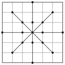
Figure 1: Illustration of the D2Q17 lattice. Each discrete velocity is represented by the length and direction of the line connecting the origin of coordinate and the corresponding dotted point.

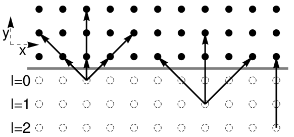
Figure 2: Illustration of the arrangement of the ghost grid and the corresponding outgoing discrete velocity (arrow at bottom for the D2Q17 model (see Fig.1). The point denotes the bulk grid while the dashed circle represents the ghost grid.

We restrict to the Couette flow within the slip-flow regime, so we may be able to use solutions of the Navier-Stokes-Fourier (NS) equations as reference. For the NS solutions, it is necessary to apply the velocity-slip and temperature-jump boundary conditions so that the velocity and temperature profiles can be written as

$$U_{NS}=\frac{(2y-1)}{2Kn+1}U_{w},$$ (13)

and

$$T_{NS}=\frac{Kn\left(8C_{p}T_{w}+5u_{w}^{2}\right)+8C_{p}T_{w}Kn^{2}+2C_{p}T_{w}-4PrU_{w}(Y-1)Y}{2C_{p}\left(2Kn+1\right)^{2}},$$ (14)

where the Knudsen number is defined as

$$Kn=\sqrt{\frac{\pi}{2}}\frac{\mu_{0}\sqrt{RT_{0}}}{p_{0}L}.$$ (15)

$U_{w}$ denotes magnitude of the component of interest of the wall velocity $\bm{u}_{w}$. For some relatively larger Knudsen numbers we may also compare to the solution of the linearized Boltzmann-BGK (L-BGK) equation.

We first evaluate the D2Q17 and D2Q16 models for isothermal flows which are presented in Fig.3 and 4, where $U_{w}$ is set to be $0.05$. Both models are simulated with $100$ computational grids in the direction of interest and the comparisons are made against the NS solutions for $Kn<0.05$ and the L-BGK solutions for $Kn\geq 0.05$ respectively. The results show that the boundary condition Eq.(12) works correctly for the isothermal flows. For $Kn\leq 0.05$, the velocity profiles are captured well by the D2Q17 model while some deviations from the L-BGK results are observed for larger Knudsen numbers, particularly at $Kn=0.1$ (see Fig.3). However, this is of no surprise as it is known that these deviations are due to the lattice structureMeng and Zhang (2011b). A further comparison to the finite difference (FD) implementation of Eq.(1) (see the description in Meng and Zhang (2011b), where the numerical simulation is validated by the analytical solution in Ansumali et al. (2007)), confirms the appropriateness of the boundary implementation. Interestingly, the D2Q16 model can given much better predictions for the velocity profile. Even at $Kn=0.5$, it still gives satisfactory results, see Fig. 4. The reason was already discussed in Meng and Zhang (2011b)

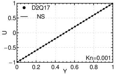
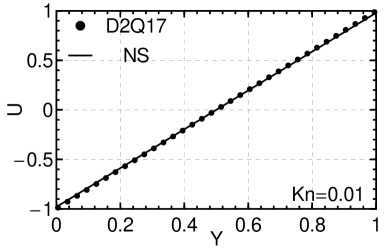
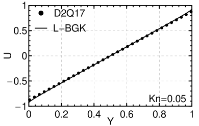
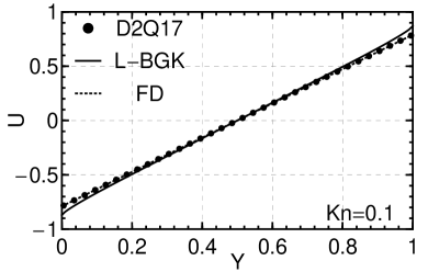
Figure 3: The velocity profiles for the isothermal cases with the D2Q17 model. The velocity is further normalized by the wall velocity.

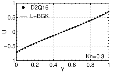
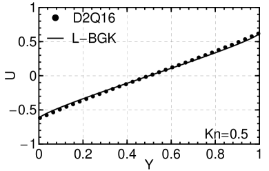
Figure 4: The velocity profiles for the isothermal cases with the D2Q16 model. The velocity is further normalized by the wall velocity.

For further validation, we also simulate the thermal Couette flows using the D3Q121 model. For these flows the relevant parameters are $C_{p}=5/2$ and $Pr=1$ while the wall temperatures are set to be $1$ and their speed $U_{w}$ is set to be $0.2$. As relatively small Knudsen numbers are considered here, the results are compared to the NS solutions, see Fig.5. The subtle temperature jumps are well captured at the wall boundary. These agreements again confirm the appropriateness of the boundary treatment. The velocity profiles show similar behavior to the isothermal cases, so they are not presented in Fig. 5.

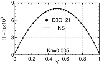
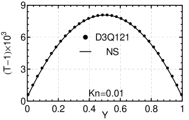
Figure 5: The temperature profiles for the thermal cases with $U_{w}=0.2$.

To evaluate the numerical accuracy, a convergence study is conducted for the thermal case of $Kn=0.01$. The simulations are run for six different grid resolutions $N_{G}=20,50,100,200,500,1000$ in the direction of interest. The results of $N_{G}=1000$ is then chosen as reference and the global relative errors of the velocity and temperature are defined as

$$E_{U}=\sqrt{\frac{\sum_{j=1}^{N_{G}}[U_{j}(Y_{j})-U_{\Delta}(Y_{j})]^{2}}{\sum_{j=1}^{N_{G}}U_{\Delta}^{2}(Y_{j})}},$$ (16)

and

$$E_{T}=\sqrt{\frac{\sum_{j=1}^{N_{G}}[T_{j}(Y_{j})-T_{\Delta}(Y_{j})]^{2}}{\sum_{j=1}^{N_{G}}(T_{\Delta}(Y_{j})-T_{w})^{2}}},$$ (17)

where $U_{\Delta}$ and $T_{\Delta}$ represent the results of $N_{G}=1000$. Fig.6 shows that the second order accuracy is achieved globally.

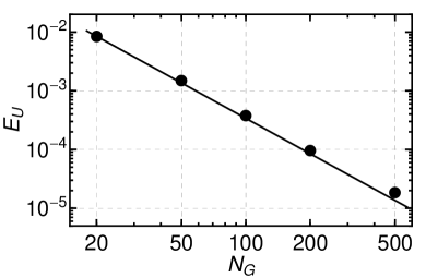
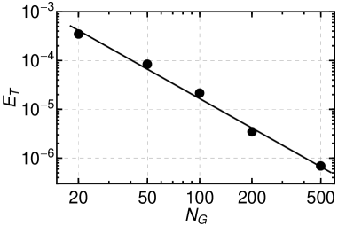
Figure 6: Dependence of the $E_{U}$ and $E_{T}$ on the grid number $N_{G}$.

V Concluding remarks

To conclude, we have formulated the kinetic diffuse reflection boundary condition for high-order LB models with emphasis on retaining the “streaming-collision” mechanism. The numerical tests for both isothermal and thermal Couette flows show that the present boundary condition can capture velocity-slip and temperature-jump very well within the capacity of the corresponding lattices. In term of numerical accuracy, we show that the second order accuracy can be achieved globally.