Extinction times for a birth-death process with weak competition

Abstract

We consider a birth-death process with the birth rates $i\lambda$ and death rates $i\mu+i(i-1)\theta$, where $i$ is the current state of the process. A positive competition rate $\theta$ is assumed to be small. In the supercritical case when $\lambda>\mu$ this process can be viewed as a demographic model for a population with a high carrying capacity around $\lambda-\mu\over\theta$.

The article reports in a self-contained manner on the asymptotic properties of the time to extinction for this logistic branching process as $\theta\to 0$. All three reproduction regimes $\lambda>\mu$, $\lambda<\mu$, and $\lambda=\mu$ are studied.

Published in Lithuanian Mathematical Journal, Vol. 53, No. 2, April, 2013, pp. 220–234

Mathematics Subject Classification: 60J80

Keywords: Birth-death process, carrying capacity, time to extinction, coupling method, logistic branching process

1 Introduction

One of the basic population models with continuous time is the linear birth-death process $(X_{0}(t),t\geq 0)$ with fixed birth and death rates $\lambda$ and $\mu$ per individual. This is a simple example of a branching process describing a population of independently reproducing individuals having three different reproductive regimes: supercritical ($\lambda>\mu$), critical ($\lambda=\mu$), and subcritical ($\lambda<\mu$).

The properties of the linear birth-death process $X_{0}(\cdot)$ and its time to extinction $\tau_{0}$ are well-known, see for example [5, pp. 270-2]. In particular,

$$\mathbb{E}_{m}X_{0}(t)=me^{(\lambda-\mu)t}$$

and

$$\mathbb{P}_{m}(\tau_{0}\leq t)=\left\{\begin{array}[]{cl}\left(\frac{\mu(1-e^{(\mu-\lambda)t})}{\lambda-\mu e^{(\mu-\lambda)t}}\right)^{m},&\mbox{in the sub- and supercritical cases,}\\ (\frac{\lambda t}{1+\lambda t})^{m},&\mbox{in the critical case,}\end{array}\right.$$

where $\mathbb{P}_{m}(\cdot)$ and $\mathbb{E}_{m}(\cdot)$ stand for the conditional probability and expectation given that the corresponding birth-death process starts from the state $m$. It follows that in the supercritical and critical cases $\mathbb{E}_{m}(\tau_{0})=\infty$ and in the subcritical case $\mathbb{E}_{m}(\tau_{0})<\infty$. Letting $t\to\infty$ one obtains the extinction probabilities

$$\mathbb{P}_{m}(\tau_{0}<\infty)=\left\{\begin{array}[]{cl}1,&\mbox{in the subcritical and critical cases,}\\ (\frac{\mu}{\lambda})^{m},&\mbox{in the supercritical case.}\end{array}\right.$$

Moreover, it is easy to see that in the subcritical case

$$\mathbb{P}_{m}\left(\tau_{0}\leq{\ln m+\ln(1-\lambda/\mu)+x\over\mu-\lambda}\right)\to e^{-(e^{-x})},\ \ m\to\infty,$$ (1)

and in the critical case

$$\mathbb{P}_{m}\left(\tau_{0}\leq mx\right)\to\exp\{-(\lambda x)^{-1}\},\ \ m\to\infty.$$ (2)

The absence of competition among individuals is a major weakness of the linear birth-death population model. A natural modification of this simple-minded model is to introduce extra deaths due to competition. We consider an indexed birth-death process $(X_{\theta}(t),t\geq 0)$ taking non-negative integer values $i\in\{0,1,2,...\}$ and having time homogenous jump rates

$$\left\{\begin{array}[]{ll}\mathbb{P}_{i}(X_{\theta}(t)=i+1)=\lambda_{i}t+o(t),&\mbox{with }\lambda_{i}=i\lambda,\\ \mathbb{P}_{i}(X_{\theta}(t)=i-1)=\mu_{i}t+o(t),&\mbox{with }\mu_{i}=i\mu+i(i-1)\theta,\\ \mathbb{P}_{i}(X_{\theta}(t)=i)=1-(\lambda_{i}+\mu_{i})t+o(t),&\end{array}\right.$$ (6)

as $t\to 0$. The key parameters $(\lambda,\mu,\theta)$ of the model are the birth, death, and competition rates providing the following description of the demographic dynamics until the process hits the absorption state $i=0$.

Given the current population size $i\geq 1$, the next change in the population size is caused either by a birth or by a death of a particle. It is assumed that coexisting particles give birth independently of each other at rate $\lambda$ per particle, so that interaction among particles does not influence birth events. Particle death is modeled by two parameters: parameter $\mu$ gives the death rate per particle ”due to natural causes” and parameter $\theta$, usually assumed to be small, quantifies the death rate due to competition pressure (factor $i(i-1)$ appearing in front of $\theta$ represents the number of pairs of competing particles). Putting $\theta=0$ brings us back to the linear birth-death process $X_{0}(\cdot)$ mentioned in the Introduction.

The process $X_{\theta}(\cdot)$ is an example of the so called logistic branching process studied in [10] along with its continuous state counterpart. The birth-death framework allows for a more detailed analysis in this special case. The most conspicuous new feature of $X_{\theta}(\cdot)$ compared to the linear birth-death process $X_{0}(\cdot)$ is the existence of a threshold value

$$i_{\theta}=\lfloor{\lambda-\mu\over\theta}\rfloor+1$$ (7)

in the supercritical case. Obtained from the equation $\lambda_{i}\approx\mu_{i}$ the threshold value $i_{\theta}$ splits the state space in two parts. For $i<i_{\theta}$ the process $X_{\theta}(\cdot)$ tends to grow while for $i>i_{\theta}$ it tends to decrease. A relevant biological interpretation of this threshold value is the carrying capacity of the environment for the population in question.

In Section 2 we summarise some useful properties of the time-homogeneous birth-death processes. It follows, in particular, that the quadratic form of the death rate compared to the linear birth rate ensures that our birth-death process with competition goes extinct with probability one (in contrast with a supercritical linear birth-death process which never dies out with a positive probability). One of the most interesting characteristics of the process $X_{\theta}(\cdot)$ is the random time to extinction $\tau_{\theta}$.

If $\theta$ is small, the competition component $i(i-1)\theta$ is much smaller than $i\mu$ for $i\ll\theta^{-1}$, so that the process $X_{\theta}(\cdot)$ at relatively low levels can be approximated by the linear birth-death process $X_{0}(\cdot)$ with parameters $(\lambda,\mu)$ and the same initial state $X_{0}(0)=m$. This is done using a coupling construction presented in Section 3.

Section 4 presents the main asymptotic results for expected value and distribution of the time to extinction $\tau_{\theta}$ as $\theta\to 0$. The remaining sections contain the proofs.

2 General properties of time homogeneous birth-death processes

Next we give a short summary of useful results for a time homogeneous birth-death process with birth rates $\lambda_{i}$ and death rates $\mu_{i}$, some of these properties can be found in [6] and [7]. An important probability

$$Q_{i}=\mathbb{P}_{i}(\mbox{reach $i+1$ before }0)$$

satisfies a recursion

$$Q_{i}={\lambda_{i}\over\lambda_{i}+\mu_{i}}+{\mu_{i}\over\lambda_{i}+\mu_{i}}Q_{i-1}Q_{i}$$

implying

$${1\over 1-Q_{i}}=1+{\lambda_{i}\over\mu_{i}}{1\over 1-Q_{i-1}}.$$

Using notation

$$\pi_{0}=1,\ \pi_{j}={\mu_{1}\cdots\mu_{j}\over\lambda_{1}\cdots\lambda_{j}},\ \Pi_{0}=0,\ \Pi_{k}=\sum_{j=0}^{k-1}\pi_{j}$$

we derive $Q_{i}=\frac{\Pi_{i}}{\Pi_{i+1}}$.

More generally, for $i\in(k,n)\subset(0,\infty)$

$$\mathbb{P}_{i}(\mbox{reach $n$ before $k$}) =\frac{\Pi_{i}-\Pi_{k}}{\Pi_{n}-\Pi_{k}},$$

$$\mathbb{P}_{i}(\mbox{reach $k$ before $n$}) =\frac{\Pi_{n}-\Pi_{i}}{\Pi_{n}-\Pi_{k}}.$$

Using this we can compute the conditional jumping probabilities

$$\mathbb{P}_{i}( \mbox{first jump goes down}|\mbox{reach $i+1$ before $k$})$$

$$={\mu_{i}\over\lambda_{i}+\mu_{i}}\frac{\mathbb{P}_{i-1}(\mbox{reach $i+1$ before $k$})}{\mathbb{P}_{i}(\mbox{reach $i+1$ before $k$})}={\mu_{i}\over\lambda_{i}+\mu_{i}}\frac{\Pi_{i-1}-\Pi_{k}}{\Pi_{i}-\Pi_{k}},$$

which in turn lead to the recursion

$$\beta_{i}^{k} \equiv\mathbb{E}_{i}(\mbox{time to reach $i+1$}|\mbox{reach $i+1$ before $k$})$$

$$={1\over\lambda_{i}+\mu_{i}}+{\mu_{i}\over\lambda_{i}+\mu_{i}}\frac{\Pi_{i-1}-\Pi_{k}}{\Pi_{i}-\Pi_{k}}(\beta_{i-1}^{k}+\beta_{i}^{k})$$

resulting in a difference equation

$$\beta_{i}^{k} ={\Pi_{i}-\Pi_{k}\over\lambda_{i}(\Pi_{i+1}-\Pi_{k})}+{\mu_{i}(\Pi_{i-1}-\Pi_{k})\over\lambda_{i}(\Pi_{i+1}-\Pi_{k})}\beta_{i-1}^{k},\ \beta_{k+1}^{k}={1\over\lambda_{k+1}+\mu_{k+1}},$$

which is easily solved as

$$\beta_{i}^{k}=\frac{\pi_{i}}{(\Pi_{i}-\Pi_{k})(\Pi_{i+1}-\Pi_{k})}\sum_{j=k+1}^{i}\frac{(\Pi_{j}-\Pi_{k})^{2}}{\lambda_{j}\pi_{j}}.$$ (8)

Similarly, for $k\in[1,i]$ the conditional jumping probabilities

$$\mathbb{P}_{k}( \mbox{first jump goes up}|\mbox{reach $k-1$ before $i+1$})$$

$$={\lambda_{k}\over\lambda_{k}+\mu_{k}}\frac{\mathbb{P}_{k+1}(\mbox{reach $k-1$ before $i+1$})}{\mathbb{P}_{k}(\mbox{reach $k-1$ before $i+1$})}={\lambda_{k}\over\lambda_{k}+\mu_{k}}\frac{\Pi_{i+1}-\Pi_{k+1}}{\Pi_{i+1}-\Pi_{k}},$$

give the recursion

$$\beta_{k}^{i+1} \equiv\mathbb{E}_{k}(\mbox{ time to reach $k-1$}|\mbox{reach $k-1$ before $i+1$})$$

$$={1\over\lambda_{k}+\mu_{k}}+{\lambda_{k}\over\lambda_{k}+\mu_{k}}\frac{\Pi_{i+1}-\Pi_{k+1}}{\Pi_{i+1}-\Pi_{k}}(\beta_{k+1}^{i+1}+\beta_{k}^{i+1})$$

resulting in a difference equation

$$\beta_{k}^{i+1} =\frac{\Pi_{i+1}-\Pi_{k}}{\mu_{k}(\Pi_{i+1}-\Pi_{k-1})}+{\lambda_{k}\over\mu_{k}}\frac{\Pi_{i+1}-\Pi_{k+1}}{\Pi_{i+1}-\Pi_{k-1}}\beta_{k+1}^{i+1},\ \ \beta_{i}^{i+1}={1\over\lambda_{i}+\mu_{i}},$$

which implies

$$\beta_{k}^{i+1}=\frac{\pi_{k-1}}{(\Pi_{i+1}-\Pi_{k-1})(\Pi_{i+1}-\Pi_{k})}\sum_{j=k}^{i}\frac{(\Pi_{i+1}-\Pi_{j})^{2}}{\lambda_{j}\pi_{j}}.$$ (9)

Observe that for all $v>u\geq 0$ relations (8) and (9) bring

$$\sum_{i=u+1}^{v}\beta_{i}^{u}=\sum_{k=u+1}^{v}\beta_{k}^{v+1}=\sum_{j=u+1}^{v}\frac{(\Pi_{v+1}-\Pi_{j})(\Pi_{j}-\Pi_{u})}{\lambda_{j}\pi_{j}(\Pi_{v+1}-\Pi_{u})}.$$ (10)

This is a confirmation (in terms of the first moments) of the statement in [11] claiming that the corresponding conditional hitting times are equal in distribution.

The expected absorption time is given by the formula

$$\mathbb{E}_{i}(\mbox{time to reach 0}) =\sum_{j=0}^{i-1}\pi_{j}\sum_{k=j+1}^{\infty}\frac{1}{\lambda_{k}\pi_{k}}=\sum_{k=1}^{\infty}\frac{\Pi_{k\wedge i}}{\lambda_{k}\pi_{k}}.$$ (11)

Indeed, if we denote the last expectation by $\alpha_{i}$, then the following recursion

$$\alpha_{i}=\frac{1}{\lambda_{i}+\mu_{i}}+\frac{\lambda_{i}}{\lambda_{i}+\mu_{i}}\alpha_{i+1}+\frac{\mu_{i}}{\lambda_{i}+\mu_{i}}\alpha_{i-1},$$

takes place with $\alpha_{0}=0$. From this recursion it is straightforward to derive formula (11). It follows from (11) that

$$\mathbb{E}_{i}(\mbox{time to reach $i-1$})=\pi_{i-1}\sum_{k=i}^{\infty}\frac{1}{\lambda_{k}\pi_{k}}.$$ (12)

In particular, for the subcritical linear birth-death process formula (11) gives

$$\mathbb{E}_{m}(\tau_{0}) ={1\over\mu-\lambda}\left(\sum_{k=1}^{m}{1-s^{k}\over k}+(s^{-m}-1)\sum_{k=m+1}^{\infty}{s^{k}\over k}\right)$$

$$={1\over\mu-\lambda}\left(\sum_{k=1}^{m}k^{-1}+\ln(1-s)+s^{-m}\sum_{k=m+1}^{\infty}{s^{k}\over k}\right),$$

with $s=\lambda/\mu$, implying

$$\mathbb{E}_{m}(\tau_{0}) ={\ln m+\gamma+\ln(1-\lambda/\mu)\over\mu-\lambda}+o(1),\ m\to\infty,$$ (13)

where $\gamma=0,577...$ is Euler’s constant. This complements the weak convergence (1) in terms of asymptotic equality of the corresponding expectations.

3 A coupling to the linear birth-death process

To partially extrapolate the nice properties of the linear birth-death process $X_{0}(\cdot)$ to the process with interaction $X_{\theta}(\cdot)$ one can use the following coupling construction (cf [1]).

Consider a bivariate Markov process $(\widehat{X}_{\theta}(\cdot),\widehat{X}_{0}(\cdot))$ with transition rates given in the next list.

Type of transition $(0\leq i<j)$	Transition rate
$(i,i)\to(i+1,i+1)$	$\lambda i$
$(i,i)\to(i-1,i-1)$	$\mu i$
$(i,i)\to(i-1,i)$	$\theta i(i-1)$
$(i,j)\to(i+1,j)$	$\lambda i$
$(i,j)\to(i-1,j)$	$\mu i+\theta i(i-1)$
$(i,j)\to(i,j+1)$	$\lambda j$
$(i,j)\to(i,j-1)$	$\mu j$

The process is constructed in such a way that $\widehat{X}_{\theta}(t)\leq\widehat{X}_{0}(t)$ for all $t\geq 0$, and the marginal distributions of $(\widehat{X}_{\theta}(\cdot),\widehat{X}_{0}(\cdot))$ coincide with those of $X_{\theta}(\cdot)$ and $X_{0}(\cdot)$, respectively.

An important question here is how long this bivariate process stays at the diagonal if $(\widehat{X}_{\theta}(0),\widehat{X}_{0}(0))=(m,m)$. Let $\kappa_{\theta}$ be the number of jumps of the process $(\widehat{X}_{\theta}(\cdot),\widehat{X}_{0}(\cdot))$ until separation, if the components stay together until extinction we put $\kappa_{\theta}=\infty$. We show below that

$$\mathbb{P}_{(m,m)}(\kappa_{\theta}\leq n)\leq\frac{(m+n)n\theta}{\lambda+\mu},$$ (14)

where $\mathbb{P}_{(m,m)}(\cdot)$ stands for the probability conditioned on the bivariate process starting from the state $(m,m)$.

Suppose $\theta\to 0$ and the starting level $m$ is fixed. In the subcritical and critical cases the total number of births and deaths in the linear birth-death processes is almost surely finite and due to (14) we may conclude that $\tau_{\theta}\rightarrow\tau_{0}$ almost surely. Moreover, since a supercritical branching process conditioned on extinction behaves like a subcritical branching process, we obtain that $\tau_{\theta}\rightarrow\tau_{0}$ almost surely provided $\tau_{0}<\infty$. This observation is summarised in the next section as a part of Theorem 4.1.

To prove (14) observe that

$$\kappa_{\theta}=\inf\{k:U_{k}\neq V_{k}\},$$

where $(U_{k},V_{k})_{k\geq 0}$ are the consecutive states visited by of the process $(\widehat{X}_{\theta}(\cdot),\widehat{X}_{0}(\cdot))$. Note that the only way for the bivariate process to get off the diagonal is the move $(i,i)\to(i-1,i)$ having the probability $\theta(i-1)\over\lambda+\mu+\theta(i-1)$ which is negligible, if the current level $i$ is not too high. Since

$$\mathbb{P}_{(m,m)}(\kappa_{\theta}=n|\kappa_{\theta}>n-1) =\sum_{i=1}^{m+n-1}\frac{\theta(i-1)}{\lambda+\mu+\theta(i-1)}\mathbb{P}_{(m,m)}(U_{n-1}=i)$$

$$\leq\frac{\theta}{\lambda+\mu}\mathbb{E}_{(m,m)}U_{n-1}\leq\frac{(m+n)\theta}{\lambda+\mu},$$

we derive (14)

$$\mathbb{P}_{(m,m)}(\kappa_{\theta}\leq n) =1-\prod_{k=1}^{n}\mathbb{P}_{(m,m)}(\kappa_{\theta}>k|\kappa_{\theta}>k-1)$$

$$\leq\sum_{k=1}^{n}\frac{(m+k)\theta}{\lambda+\mu}\leq\frac{(m+n)n\theta}{\lambda+\mu}.$$

4 Main Results

We claim that as $\theta\to 0$ the following two limit theorems hold for the birth-death process defined by (6).

 Theorem 4.1

If $X_{\theta}(0)=m$, where $m$ is a fixed positive integer, then

(i) in the subcritical and critical cases when $\lambda\leq\mu$

$$\mathbb{P}_{(m,m)}(\tau_{\theta}\rightarrow\tau_{0})=1,$$

(ii) in the supercritical case when $\lambda>\mu$

$$\mathbb{P}_{(m,m)}(\tau_{\theta}\rightarrow\tau_{0}|\tau_{0}<\infty)=1,$$

and for any $x\geq 0$

$$\mathbb{P}_{(m,m)}(\tau_{\theta}>xc_{1}\sqrt{\theta}\,e^{c_{2}/\theta})|\tau_{0}=\infty)\rightarrow e^{-x},$$

where

$$c_{1}=\lambda(\lambda-\mu)^{-2}\sqrt{2\pi/\mu},\hskip 14.22636ptc_{2}=\lambda-\mu-\mu\ln(\lambda/\mu).$$ (15)

Theorem 4.1 (i) and the first part of (ii) are proven in the previous section. The proof of the second part of Theorem 4.1 (ii) is given after the proof of the first part of the next theorem.

 Theorem 4.2

If $X_{\theta}(0)=m_{\theta}$ and $\theta m_{\theta}\rightarrow a>0$, then

(i) in the supercritical case when $\lambda>\mu$

$$\mathbb{E}_{m_{\theta}}(\tau_{\theta})\sim c_{1}\sqrt{\theta}\,e^{c_{2}/\theta}$$

with positive constants $c_{1}$, $c_{2}$ given by (15), and for any $x\geq 0$

$$\mathbb{P}_{m_{\theta}}(\tau_{\theta}>xc_{1}\sqrt{\theta}\,e^{c_{2}/\theta})\rightarrow e^{-x},$$

(ii) in the subcritical case when $\lambda<\mu$

$$\mathbb{E}_{m_{\theta}}(\tau_{\theta})={\ln(a\theta^{-1})+\ln{\mu-\lambda\over\mu}+\ln{\mu-\lambda\over\mu-\lambda+a}+\gamma\over\mu-\lambda}+o(1),$$ (16)

and for any $x\geq 0$

$$\mathbb{P}_{m_{\theta}}\left(\tau_{\theta}\leq{\ln(a\theta^{-1})+\ln{\mu-\lambda\over\mu}+\ln{\mu-\lambda\over\mu-\lambda+a}+x\over\mu-\lambda}\right)\rightarrow e^{(-e^{-x})}.$$ (17)

(iii) in the critical case when $\lambda=\mu$

$$\mathbb{E}_{m_{\theta}}(\tau_{\theta})\sim{(\pi/2)^{3/2}\over\sqrt{\theta\mu}}.$$

The asymptotic formulae for $\mathbb{E}_{m_{\theta}}(\tau_{\theta})$ in Theorem 4.2 (ii), (iii) are verified by simulations as shown in Figures 1, 2. Comparing the asymptotic formula (13) for the linear birth-death process to the that for the process with competition (16) we see that as $\theta\to 0$ and $\theta m_{\theta}\to a$ the average survival time reduces by

$$\mathbb{E}_{m_{\theta}}(\tau_{0})-\mathbb{E}_{m_{\theta}}(\tau_{\theta})\to{1\over\mu-\lambda}\ln{\mu-\lambda+a\over\mu-\lambda}.$$

As one would expect, this difference becomes small for larger values of $\mu$ and/or smaller values of $a$.

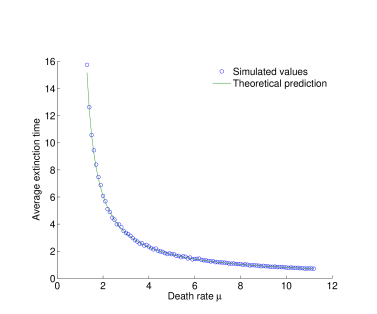
Figure 1: Averages of 100 simulations for each value of the death rate are plotted against the values predicted by Theorem 4.2 (ii). Choice of parameters: initial population size $m_{\theta}=1000$, competition strength $\theta=0.001$, and birth rate $\lambda=1$.

Notice that Theorem 4.2 (ii) provides with a counterpart of the weak convergence (1) for the linear birth-death processes, however, we could not find a counterpart of (2) in the critical case. The following lemma plays a crucial role in the asymptotic analysis of all three cases.

 Lemma 4.3

For our particular model the function $\pi_{j}=\prod_{i=0}^{j-1}{\mu+\theta i\over\lambda}$ satisfies the approximation

$$\pi_{j}=(1+j\theta/\mu)^{-1/2}\,e^{-W(j\theta)/\theta}(1+\eta_{j}(\theta)),\ j\geq 1,$$ (18)

where $W(x)=x-x\ln\frac{\mu+x}{\lambda}-\mu\ln\frac{\mu+x}{\mu}$ and for any fixed $T>0$

$$\sup_{1\leq j\leq T/\theta}\left|\eta_{j}(\theta)\right|\to 0,\ \ \theta\to 0.$$

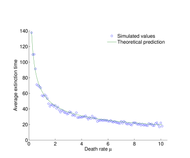
Figure 2: Averages of 100 simulations for $m_{\theta}=1000$, $\theta=0.001$ are plotted against the values predicted by Theorem 4.2 (iii).

Proof Observe that

$$\theta\ln\pi_{j} =\theta\sum\limits_{k=0}^{j-1}\ln\frac{\mu+k\theta}{\lambda}$$

$$=\int_{0}^{j\theta}\!\ln\frac{\mu+y}{\lambda}\,\mathrm{d}y-\sum_{k=0}^{j-1}\int_{k\theta}^{(k+1)\theta}\ln\frac{\mu+y}{\mu+k\theta}\,dy$$

$$=-W(j\theta)-\frac{\theta}{2}\sum_{k=0}^{j-1}\frac{\theta}{\mu+k\theta}+O(j\theta^{3}).$$

It remains to verify that

$$\sup_{j\geq 0}\left|\prod_{k=0}^{j}e^{-{\theta\over\mu+k\theta}}-{\mu\over\mu+j\theta}\right|\to 0.$$

$\Box$

5 Proofs for the supercritical case

In this section we first prove Theorem 4.2 (i) and then Theorem 4.1 (ii) borrowing key ideas from [1].

We start by considering the supercritical $X_{\theta}(\cdot)$ with the initial state $X_{\theta}(0)=i_{\theta}$ given by (7). It will take a geometric number $K_{\theta}\sim{\rm Geom}(1-Q_{i_{\theta}})$ of returns to the initial state from above before the extinction event. Let $\tau_{\theta}^{\prime}$ be the time needed for $X_{\theta}(\cdot)$ to enter the level $i_{\theta}$ from above, and $\tau_{\theta}^{\prime\prime}$ be the absorption time counted from the last entrance moment to the state $i_{\theta}$ from above. If there were no visits of $i_{\theta}$ from above, we put $\tau_{\theta}^{\prime}=\tau_{\theta}$ and $\tau_{\theta}^{\prime\prime}=0$. Clearly, $\tau_{\theta}$ is the sum of $\tau_{\theta}^{\prime}$, $\tau_{\theta}^{\prime\prime}$, and of $K_{\theta}$ independent durations of the corresponding excursions. It follows that the statement (ii) of Theorem 4.2 is a straightforward consequence of the next three lemmata.

 Lemma 5.1

In the supercritical case as $\theta\to 0$

$$1-Q_{i_{\theta}}\sim\frac{(\lambda-\mu)\sqrt{\mu}}{\lambda^{3/2}}e^{-c_{2}/\theta}.$$ (19)

 Lemma 5.2

In the supercritical case the expected duration $M_{\theta}$ of an excursion starting from $i_{\theta}$ and returning to $i_{\theta}$ from above satisfies

$$M_{\theta}\sim\sqrt{\frac{2\pi\theta}{\lambda}}\frac{1}{\lambda-\mu},\ \theta\to 0.$$

 Lemma 5.3

Under the assumptions of Theorem 4.2 (i) for any fixed positive $\epsilon$

$$\mathbb{E}_{m_{\theta}}(\tau_{\theta}^{\prime})=o(e^{\epsilon/\theta}),\ \ \mathbb{E}_{m_{\theta}}(\tau_{\theta}^{\prime\prime})=o(e^{\epsilon/\theta}),\ \ \theta\to 0.$$

Proof of Lemma 5.1. It is shown in Section 2 that $1-Q_{i_{\theta}}=\frac{\pi_{i_{\theta}}}{\Pi_{i_{\theta}+1}}$. According to Lemma 4.3

$$\pi_{i_{\theta}}\sim\sqrt{\mu\over\lambda}\,e^{-c_{2}/\theta},$$ (20)

and in view of $\Pi_{i_{\theta}}\to\frac{\lambda}{\lambda-\mu}$ we arrive at (19).

$\Box$

Proof of Lemma 5.2. We show first that

$$\sum_{j=1}^{\infty}\frac{1}{\lambda_{j}\pi_{j}}\sim\frac{1}{(\lambda-\mu)\sqrt{\mu}}\sqrt{2\pi\theta}e^{c_{2}/\theta}$$ (21)

by dividing the left sum in two parts using the threshold $l_{\theta}=\lceil{2\lambda-\mu\over\theta}\rceil$. Observe that by definitions of $i_{\theta}$ and $l_{\theta}$ we have $\pi_{j}\geq\pi_{i_{\theta}}\cdot 2^{j-l_{\theta}}$ for $j>l_{\theta}$. Thus applying (20) we obtain

$$\sum_{j=l_{\theta}+1}^{\infty}\frac{1}{\lambda_{j}\pi_{j}}=O(\theta/\pi_{i_{\theta}})=O(\theta e^{c_{2}/\theta}).$$

On the other hand, due to (18)

$$\sum_{j=1}^{l_{\theta}}\frac{1}{j\pi_{j}}\sim\int_{0}^{2\lambda-\mu}\frac{\sqrt{\mu+s}}{s\sqrt{\mu}}e^{W(s)/\theta}ds.$$

As the function $W(\cdot)$ has its maximum over the integration interval at the point $\lambda-\mu$ we conclude using the Laplace method that

$$\sum_{j=1}^{l_{\theta}}\frac{1}{\lambda_{j}\pi_{j}}\sim\frac{\sqrt{2\pi\theta}e^{c_{2}/\theta}}{(\lambda-\mu)\sqrt{\mu}}$$

completing the proof of (21).

Combining (8) and (12) we get

$$M_{\theta}=\pi_{i_{\theta}}\sum_{k=1}^{\infty}\frac{\psi_{k}(i_{\theta})}{\lambda_{k}\pi_{k}},\mbox{ where }\psi_{k}(i)=\min\left\{\frac{\Pi_{k}^{2}}{\Pi_{i}\Pi_{i+1}},1\right\}$$

Relations (20) and (21) give

$$\pi_{i_{\theta}}\sum_{k=1}^{\infty}\frac{1}{\lambda_{k}\pi_{k}}\sim\sqrt{\frac{2\pi\theta}{\lambda}}\frac{1}{\lambda-\mu},$$

and it remains only to observe that $\psi_{k}(i_{\theta})\to 1$ uniformly over $k$ larger than $\epsilon/\theta$ however small is a fixed positive $\epsilon$.

$\Box$

Proof of Lemma 5.3. Notice that due to (10)

$$E(\tau_{\theta}^{\prime\prime})<\mathbb{E}_{i_{\theta}}(\mbox{time to reach 0 }|\mbox{ reach 0 before $i_{\theta}+1$})=\sum_{k=1}^{i_{\theta}}\beta_{k}^{i_{\theta}+1}=o(e^{\epsilon/\theta}).$$

On the other hand, for $m_{\theta}\leq i_{\theta}$

$$\mathbb{E}_{m_{\theta}}(\tau_{\theta}^{\prime}) <\mathbb{E}_{1}(\mbox{time to reach $i_{\theta}+1$ }|\mbox{ reach $i_{\theta}+1$ before 0})$$

$$\hskip 14.22636pt+\mathbb{E}_{i_{\theta}+1}(\mbox{time to reach $i_{\theta}$})$$

$$=\sum_{i=1}^{i_{\theta}}\beta_{i}^{0}+\pi_{i_{\theta}}\sum_{k=i_{\theta}+1}^{\infty}\frac{1}{\lambda_{k}\pi_{k}}=o(e^{\epsilon/\theta}),$$

and for $m_{\theta}>i_{\theta}$

$$\mathbb{E}_{m_{\theta}}(\tau_{\theta}^{\prime}) =\mathbb{E}_{m_{\theta}}(\mbox{time to reach $i_{\theta}$})=\sum_{k=i_{\theta}+1}^{\infty}\frac{\Pi_{k\wedge m_{\theta}}-\Pi_{i_{\theta}}}{\lambda_{k}\pi_{k}}=o(e^{\epsilon/\theta}).$$

$\Box$

Proof of Theorem 4.1 (ii). Put

$$S_{\theta}(\delta)=\inf\{t\geq 0:\widehat{X}_{0}(t)\geq\delta/\theta\}.$$

In view of the previous analysis it is enough to show that for some fixed $\delta\in(0,{\lambda-\mu\over\mu})$

$$\mathbb{P}_{(m,m)}(\tau_{\theta}>S_{\theta}(\delta)|\tau_{0}=\infty)\rightarrow 1.$$

We verify this by showing that for some fixed $\alpha\in(0,\frac{1}{2})$, $\rho\in(0,\frac{\lambda-\mu}{\lambda+\mu})$

$$\mathbb{P}_{(m,m)}(\tau_{\theta}>S_{\theta}(\rho\theta^{1-\alpha})|\tau_{0}=\infty)\rightarrow 1,$$ (22)

and

$$\mathbb{P}_{m}(\tau_{\theta}>S_{\theta}(\delta)|\tau_{\theta}>S_{\theta}(\rho\theta^{1-\alpha}))\rightarrow 1.$$ (23)

According to (14) we have

$$\mathbb{P}_{(m,m)}(U_{k}=V_{k},k=0,\ldots,\theta^{-\alpha}|\tau_{0}=\infty)\rightarrow 1.$$

Note that

$$\mathbb{P}_{m}(V_{\theta^{-\alpha}}\geq\rho\theta^{-\alpha}|V_{k}\neq 0;1\leq k\leq\theta^{-\alpha})\rightarrow 1,$$

since under the condition of non-extinction $V_{n}$ is just a simple random walk restricted to the set of positive integers, having a drift that is bounded from below by $\frac{\lambda-\mu}{\lambda+\mu}>0$. Combining the last two relations we arrive at (22).

Finally, (23) follows from the fact that the probability

$$\mathbb{P}_{i}(\mbox{reach $n$ before $0$})={\Pi_{i}}/{\Pi_{n}}$$

with $i=\rho\theta^{-\alpha}$ and $n=\delta/\theta$ tends to one as $\theta\to 0$.

$\Box$

6 Proof of Theorem 4.2 (ii)

In the subcritical case $s=\lambda/\mu$ lies in $(0,1)$. To establish the approximation formula (16) we refer to (11) which gives

$$\mathbb{E}_{m}(\tau_{\theta}) =\sum_{j=0}^{m-1}\sum_{k=j+1}^{\infty}\frac{\pi_{j}}{\lambda k\pi_{k}}=\lambda^{-1}\sum_{j=0}^{m-1}\sum_{k=j+1}^{\infty}\frac{s^{k-j}}{k}\cdot r_{j}\cdots r_{k-1},$$

where $r_{i}={\mu\over\mu+i\theta}$, and on the other hand,

$$\mathbb{E}_{m}(\tau_{0}) =\lambda^{-1}\sum_{j=0}^{m-1}\sum_{k=j+1}^{\infty}\frac{s^{k-j}}{k}.$$

Thus in view of (13) we have to verify that

$$\sum_{j=0}^{a/\theta}\sum_{k=j+1}^{\infty}\frac{s^{k-j}}{k}\cdot\big{(}1-r_{j}\cdots r_{k-1}\big{)}\to{\lambda\over\mu-\lambda}\ln{\mu-\lambda+a\over\mu-\lambda}.$$ (24)

To prove (24) choose arbitrary but fixed small $\epsilon$ and large $T$ and consider

$$\sum_{j=\epsilon/\theta}^{a/\theta}\sum_{k=j+1}^{j+T}\frac{s^{k-j}}{k}\cdot\big{(}1-r_{j}\cdots r_{k-1}\big{)} =\sum_{j=\epsilon/\theta}^{a/\theta}\sum_{k=j+1}^{j+T}\frac{s^{k-j}}{k}\cdot\big{(}1-e^{-{V(k\theta)-V(j\theta)\over\theta}}\big{)}+o(1),$$

where a counterpart of Lemma 4.3 was used with

$$V(x) =(x+\mu)\ln{x+\mu\over\mu}-x,$$

$$V(x)-V(y) =(x-y)\ln{x+\mu\over\mu}+(y+\mu)\Big{(}\ln{x+\mu\over y+\mu}-{x-y\over y+\mu}\Big{)}.$$

Due to the last equality we can replace $e^{-{V(k\theta)-V(j\theta)\over\theta}}$ with $\big{(}{\mu\over j\theta+\mu}\big{)}^{k-j}$ and get

$$\sum_{j=\epsilon/\theta}^{a/\theta}\sum_{k=j+1}^{j+T}\frac{s^{k-j}}{k}\cdot\big{(}1-r_{j}\cdots r_{k-1}\big{)} =\sum_{j=\epsilon/\theta}^{a/\theta}\sum_{l=1}^{T}\frac{s^{l}}{j}\cdot\big{(}1-(1+j\theta/\mu)^{-l}\big{)}+o(1).$$

Since

$$\sum_{l=1}^{\infty}s^{l}\big{(}1-(1+j\theta/\mu)^{-l}\big{)}={1\over 1-s}-{1\over 1-s(1+j\theta/\mu)^{-1}}={s\over 1-s}\cdot{j\theta\over\mu(1-s)+j\theta},$$

to derive (24) it remains to observe that

$$\sum_{j=\epsilon/\theta}^{a/\theta}\sum_{l=1}^{T}\frac{s^{l}}{j}\cdot\big{(}1-(1+j\theta/\mu)^{-l}\big{)}={s\over 1-s}\sum_{j=\epsilon/\theta}^{a/\theta}{\theta\over\mu(1-s)+j\theta}+\rho_{T}(\theta),$$

where

$$\limsup_{T\to\infty}\limsup_{\theta\to\infty}|\rho_{T}(\theta)|=0,$$

and

$$\sum_{j=\epsilon/\theta}^{a/\theta}{\theta\over\mu(1-s)+j\theta} \to\int_{\epsilon}^{a}\frac{dx}{\mu(1-s)+x}=\ln{\mu-\lambda+a\over\mu-\lambda+\epsilon}.$$

This finishes the proof of (16).

Next we prove the weak convergence stated in the subcritical case. Fix some $0<\alpha<\frac{1}{2}$. Following the approach of [3], we establish (17) after splitting the extinction time $\tau_{\theta}$ in two parts

$$\tau_{\theta}=\tau_{\theta,1}+\tau_{\theta,2},$$

where $\tau_{\theta,1}$ is the time for $X_{\theta}(\cdot)$ to reach the level $\theta^{-\alpha}$ and $\tau_{\theta,2}$ is the time for the process $X_{\theta}(\cdot)$ starting from $\theta^{-\alpha}$ to get absorbed at 0.

If $X_{\theta}(0)=m_{\theta}$ and $\theta m_{\theta}\rightarrow a>0$, then according to [9] the scaled process $\theta X_{\theta}(\cdot)$ converges in probability, uniformly on compact time intervals, to the deterministic motion $x(\cdot)$ governed by the differential equation

$$x^{\prime}(t)=(\lambda-\mu)x(t)-x^{2}(t),\ \ x(0)=a.$$ (25)

This equation has an explicit solution

$${1\over x(t)}=\left({1\over a}+{1\over\mu-\lambda}\right)e^{(\mu-\lambda)t}-{1\over\mu-\lambda}.$$ (26)

Solving formally $x(t)=\theta^{1-\alpha}$ for the time $t$ required for the deterministic motion to reach the low level $\theta^{1-\alpha}$ we find

$$\tau_{\theta,1}=\frac{(1-\alpha)\ln\theta^{-1}-\ln(a^{-1}+(\mu-\lambda)^{-1})}{\mu-\lambda}+o(1)$$ (27)

in probability. Combining (1) with (14) entails

$$P\left(\tau_{\theta,2}\leq{\alpha\ln\theta^{-1}+\ln(1-\lambda/\mu)+x\over\mu-\lambda}\right)\to e^{-(e^{-x})},\ \ \theta\to 0,$$

which together with (27) give (17).

The full justification of (27) can be achieved using the approach developed in [2] and [3]. It is based on an appropriate integral of the equation (25), which in our case is

$$h(z,t)=t-{\ln(\mu-\lambda+z)-\ln x+\ln a-\ln(\mu-\lambda+a)\over\mu-\lambda}.$$ (28)

If $x(t)$ satisfies (26), then $h(x(t),t)=0$ and furthermore, $x(t-h(z,t))=z$. It follows,

$$|z-x(t)|\leq(\mu-\lambda+a)x(t)|h(z,t)|.$$ (29)

For the rest of the proof we replace $a$ by $\theta m_{\theta}$ in relations (26) and (28) defining $x(t)$ and $h(x,t)$. Let $\nu_{\epsilon}$ denote the minimal $t>0$ such that $|\theta X_{\theta}(t)-x(t)|>\epsilon$, and put $H_{\theta}(t)=|h(\theta X_{\theta}(t),t)|$ so that $H_{\theta}(0)=0$. According to [3] a modified Corollary 1 of Lemma 5 in [2] gives

$$\mathbb{P}_{m_{\theta}}(H_{\theta}(t\wedge\nu_{\epsilon})>y)\leq 2\exp\{-ky+tC_{\epsilon}(\theta,k,t)\}$$

for all positive $t$ and $k$, where the function $C_{\epsilon}(\theta,k,t)$ can be chosen such that for some positive constants $C_{1},C_{2},C_{3}$

$$C(\theta,k,t)={C_{1}k\theta\over(x(t)-\epsilon)^{2}}+{C_{2}k^{2}\theta\over(x(t)-\epsilon)^{2}}\exp\left\{{C_{3}k\theta\over x(t)-\epsilon}\right\},$$

if we assume that $x(t)>\epsilon$. If furthermore, $x(t)-\epsilon>C_{4}\theta^{1-\alpha}$, then

$$C(\theta,k,t)<C_{5}k\theta^{2\alpha-1}+C_{6}k^{2}\theta^{2\alpha-1}e^{C_{7}k\theta^{\alpha}}.$$

7 Proof of Theorem 4.2 (iii)

According to (11) and (18) we have in the critical case

$$\theta\mathbb{E}_{m_{\theta}}(\tau_{\theta}) \sim\int_{0}^{a}{\sqrt{\mu+y}\over\mu y}\int_{0}^{y}{1\over\sqrt{\mu+x}}e^{W(y)-W(x)\over\theta}dxdy$$

$$\hskip 28.45274pt+\int_{a}^{\infty}{\sqrt{\mu+y}\over\mu y}e^{W(y)/\theta}dy\cdot\int_{0}^{{a}}{1\over\sqrt{\mu+x}}e^{-W(x)/\theta}dx,$$

where $W(x)=x-(\mu+x)\ln\frac{\mu+x}{\mu}$. Notice that $W(x)=-{x^{2}\over 2\mu}(1+2r(x))$, where $r(x)\to 0$ as $x\to 0$. It follows, that for any $T>0$

$${1\over\sqrt{\mu\theta}}\int_{0}^{T\sqrt{\mu\theta}} {\sqrt{\mu+y}\over\mu y}\int_{0}^{y}{1\over\sqrt{\mu+x}}e^{W(y)-W(x)\over\theta}dxdy$$

$$=\int_{0}^{T}{\sqrt{\mu+z\sqrt{\mu\theta}}\over\mu z}\int_{0}^{z}{1\over\sqrt{\mu+t\sqrt{\mu\theta}}}e^{t^{2}-z^{2}\over 2}e^{t^{2}r(t\sqrt{\mu\theta})}e^{-z^{2}r(z\sqrt{\mu\theta})}dtdz$$

$$\to\mu^{-1}\int_{0}^{T}z^{-1}\int_{0}^{z}e^{t^{2}-z^{2}\over 2}dtdz.$$

On the other hand, since for $0\leq x\leq y$

$$W(y)-W(x)\leq(x-y)\ln\frac{\mu+x}{\mu}-{(y-x)^{2}\over 2(\mu+y)},$$

we have with $C={\sqrt{\mu+a}\over\sqrt{\mu}}$

$$\int_{T\sqrt{\mu\theta}}^{a} {\sqrt{\mu+y}\over y}\int_{0}^{y}{1\over\sqrt{\mu+x}}e^{W(y)-W(x)\over\theta}dxdy$$

$$\leq C\int_{T\sqrt{\mu\theta}}^{a}y^{-1}\left(\int_{0}^{y/2}e^{-{(y-x)^{2}\over 2(\mu+a)\theta}}dx+\int_{y/2}^{y}e^{{x-y\over\theta}\ln\frac{\mu+x}{\mu}}dx\right)dy$$

$$\leq{C\over 2}\int_{T\sqrt{\mu\theta}}^{\infty}e^{-{y^{2}\over 8(\mu+a)\theta}}dy+C\int_{T\sqrt{\mu\theta}}^{a}y^{-1}\int_{y/2}^{y}e^{{x-y\over\theta}\ln\frac{\mu+y/2}{\mu}}dxdy$$

$$\leq{C\sqrt{\theta}\over 2}\int_{T\sqrt{\mu}}^{\infty}e^{-{z^{2}\over 8(\mu+a)}}dz+C\theta\int_{T\sqrt{\mu\theta}}^{a}{dy\over y\ln(1+{y\over 2\mu})},$$

where the last integral is estimated from above by a constant plus

$$\int_{T\sqrt{\mu\theta}}^{2\mu}{dy\over y\ln(1+{y\over 2\mu})} \leq\int_{T\sqrt{\theta/(4\mu)}}^{1}{dz\over z(z-{z^{2}\over 2})}\leq{2\sqrt{\mu}\over T\sqrt{\theta}}+{1\over 2}\ln\left({4\mu\over T\sqrt{\mu\theta}}\right).$$

Using a table integral

$$\int_{0}^{\infty}z^{-1}\int_{0}^{z}e^{t^{2}-z^{2}\over 2}dtdz=\left({\pi\over 2}\right)^{3/2}$$

we conclude that

$$\limsup_{\theta\to 0}\left|{1\over\sqrt{\theta}}\int_{0}^{a}{\sqrt{\mu+y}\over\mu y}\int_{0}^{y}{1\over\sqrt{\mu+x}}e^{W(y)-W(x)\over\theta}dxdy-{1\over\sqrt{\mu}}\left({\pi\over 2}\right)^{3/2}\right|\leq\epsilon_{T},$$

where $\epsilon_{T}\to 0$ as $T\to\infty$.

It remains to observe that

$$\int_{a}^{\infty}{\sqrt{\mu+y}\over\mu y}e^{W(y)/\theta}dy\cdot\int_{0}^{{a}}{1\over\sqrt{\mu+x}}e^{-W(x)/\theta}dx=o(\sqrt{\theta}).$$

Remark. Our approximations for the mean extinction time are specific to the population model we study. These should be compared with similar calculations performed in a more general setting by [4], where, however, strict justifications of some important steps are missing.

Acknowledgments. SS was supported by the Swedish Research Council grant 621-2010-5623. AS was supported by the Scientific Committee of Kazakhstan’s Ministry of Education and Science, grant 0732/GF 2012-14.

References

[1]Andersson, H., and Djehiche, B. (1998). A threshold limit theorem for the stochastic logistic epidemic. J. Appl. Prob., 35(3) : 662-670.
[2]Barbour, A.D. (1974). On a functional central limit theorem for Markov population processes. Adv. Appl. Prob., 6(1): 21-39.
[3]Barbour, A.D. (1975). The duration of closed stochastic epidemic. Biometrika, 62(2): 477-482.
[4]Doering, C.R., Sargsyan, K.V., and Sander, L.M. (2005). Extinction times for birth-death processes:exact results,continuum asymptotics, and the failure of the Fokker-Plank approximation. Multiscale Model. Simul.,
3(2): 283-299.
[5] Grimmet, G.R. and Stirzaker, D.R. (2001). Probability and Random Processes (3rd Edition). Oxford: Clarendon Press.
[6] Karlin, S., and McGregor, J. (1957). The classification of birth and death processes. Trans. Amer. Math. Soc., 86(2): 366-400.
[7] Karlin, S. and Taylor, M. (1975). A first course in stochastic processes (2nd Edition). New York: Academic Press.
[8] Keilson, J. (1979). Markov chain models-rarity and exponentiality. New York: Springer-Verlag.
[9] Kurtz, J., (1970). Solutions of ordinary differential equations as limits of pure jump Markov processes. J. Appl. Prob., 7: 49-58.
[10] Lambert, A., (2005). The branching process with logistic growth. Ann. Appl. Prob., 15: 1506-1535.
[11]Sumita,U., (1984). On conditional passage time structure of birth-death processes. J. Appl. Prob., 21(1): 10-21.