Utility Maximization in a Binomial Model with transaction costs: a Duality Approach Based on the Shadow Price Process

Abstract.

We consider the problem of optimizing the expected logarithmic utility of the value of a portfolio in a binomial model with proportional transaction costs with a long time horizon. By duality methods, we can find expressions for the boundaries of the no-trade-region and the asymptotic optimal growth rate, which can be made explicit for small transaction costs (in the sense of an asymptotic expansion). Here we find that, contrary to the classical results in continuous time, see Janeček and Shreve [Fin. Stoch. 8, 2004], the size of the no-trade-region as well as the asymptotic growth rate depend analytically on the level $\lambda$ of transaction costs, implying a linear first order effect of perturbations of (small) transaction costs, in contrast to effects of order $\lambda^{1/3}$ and $\lambda^{2/3}$, respectively, as in continuous time models. Following the recent study by Gerhold, Muhle-Karbe and Schachermayer [Fin. Stoch. 2011 (online first)] we obtain the asymptotic expansion by an almost explicit construction of the shadow price process.

1. Introduction

In this paper we consider the problem of optimal investment in a market consisting of two assets, one risk-free asset, the bond, which, for simplicity, is assumed to be constant in time and one stock. More precisely, we assume that the investor wants to maximize her expected utility from final wealth, i.e.,

$$\mathbb{E}\left[U(V_{T})\right]\to\max,$$

for a given finite horizon $T>0$, a given utility function $U$ and, certainly, a given initial wealth, say, $x$. Here, $V_{T}$ denotes the value of the portfolio obtained by the investor at time $T$. In fact, we shall only consider the case of the most tractable utility function, $U(x)=\log(x)$. In this framework, it is known since the seminal work of Merton in 1969 [Mer69] that in a frictionless market in which the price of the risky asset follows a geometrical Brownian motion (with drift $\mu$ and volatility $\sigma$), it is optimal for the investor to keep the fraction of wealth invested in the risky asset, $\varphi_{t}S_{t}$, w.r.t. the total portfolio wealth, $\varphi^{0}_{t}+\varphi_{t}S_{t}$ constant equal to $\mu/\sigma^{2}$. In particular, this means that the portfolio has to be constantly re-balanced. Of course, this result fully deserves its fame, but nonetheless it mainly implies that the model of a frictionless financial market in continuous time is not an adequate model of reality in the context of portfolio optimization, since it gives an investment strategy which would lead to immediate bankruptcy if applied in practice due to the bid-ask spread. Consequently, it is essential to study the optimal investment problem under transaction costs, a work undertaken by many authors starting with Magill and Constantinides [MC76]. While actually treating the related problem of optimizing utility from consumption, in this work the main difference to the Merton rule has already been established in a heuristic way, namely that an investor optimizing his expected utility keeps the proportion of wealth invested in the stock to total wealth inside of a fixed interval instead of fixed single point. Consequently, the investor will not trade actively while the proportion remains inside the interval, suggesting the term “no-trade-region”. On the other hand, when the proportion is about to leave the no-trade-region, then the investor will trade stocks for bonds (or conversely) so as to just keep the proportion inside the interval.

Since then, many papers in the finance and mathematical finance literature have treated the problem of portfolio optimization under proportional transaction costs, for instance [DN90], [SS94], [JS04] and [TKA88], to mention some of the most influential ones on the mathematical side. As usual for concave optimization problems, there are essentially two approaches for the analysis: the primal approach, which, in this case, is mostly based on the associated Hamilton-Jacobi-Bellman equation, and the dual approach. Representatives of the former method are the works [SS94] and [JS04], where the (asymptotic) first order effect of the transaction costs to the no-trade-region was found for the utility-from-consumption problem. An elegant formulation of the dual approach is based on the notion of shadow prices, see Kallsen and Muhle-Karbe [KMK10], and we especially mention the inspiring work of Gerhold, Muhle-Karbe and Schachermayer [GMKS11], where asymptotic expansions for the no-trade-region and the asymptotic growth rate were found in a utility-from-terminal-wealth problem. [JS04] and [GMKS11] found the characteristic result that the size of the no-trade-region is of order $\lambda^{1/3}$, where $\lambda$ is the relative bid-ask-spread.

Almost all of the literature mentioned so far studied the effects of market-friction in the form of proportional transaction costs in the case of markets allowing continuous time trading, more specifically, in a Black-Scholes model. In the context of a discrete model, the problem seems to be less pressing, as infinite trading activities are anyway not possible, which implies that the optimal portfolio strategy of a friction-less, discrete-time model is, at least, admissible in a model with transaction costs. However, also in a discrete-time market, such a portfolio will be far from optimal. We refer to [GJ94] for numerical experiments on the effects of transaction costs in a utility-from-terminal-wealth problem. A thorough analytical and numerical study of the use of dynamic programming was done by Sass [Sas05] allowing for very general structures of transaction costs, including some numerical examples. [CSS06] use the dual approach for their analysis of the value function and the optimal strategy for the super-replication problem of a derivative. In particular, when the transaction costs are large enough, they show that buy-and-hold (or sell-and-hold) strategies are optimal. In the context of super-replication, one should also mention the recent [DS11]. Last but not least, we would also like to mention [Kus95], where the convergence of the super-replication cost in a binomial model with transaction costs was studied when the binomial model converges weakly to a geometrical Brownian motion.

The goal of this paper is to derive similar asymptotic expansions of the size of the no-trade-region and the asymptotic growth rate in the binomial model. For this purpose, we are going to use the shadow price approach of [GMKS11], and, as common in this strand of research, we shall restrict our attention to the problem of a long investment horizon $T\to\infty$. We find explicit terms for the no-trade-region as well as the asymptotic optimal growth rate when the relative bid-ask-spread $\lambda$ is small, in the sense of asymptotic expansions in terms of $\lambda$. We find that, contrary to the continuous case, in a binomial model the first order effect of proportional transaction costs $\lambda$ to both the no-trade-region and the optimal growth rate is of order $\lambda$. Economically, this marked difference can be easily understood, as in a discrete-time model all-too-frequent trading is already hindered by the model itself, which does not allow infinite trading activities. Analytically, we find that the Black-Scholes model appears as a singular limit of the family of binomial models. More precisely, let us consider a family of binomial models with fixed horizon $T$ indexed by the time increment $\delta$ converging weakly on path-space to a Black-Scholes model. Then the no-trade-region depends analytically on $\lambda$ for every $\delta>0$, but in the limiting case the function is no longer differentiable, implying different first order effects. Finally, we study the convergence of the no-trade-region and the asymptotic growth rate to the corresponding quantities in the Black-Scholes model provided that $\delta$ is small compared to $\lambda$.

2. Setting

Let $\left(\Omega,\mathcal{F},P\right)$ denote a probability space large enough that we can define a binomial model $(S_{t})_{t\in\mathbb{N}}$ with infinite time horizon. Throughout the paper, the filtration $(\mathcal{F}_{t})_{t\in\mathbb{N}}$ is generated by the process $(S_{t})_{t\in\mathbb{N}}$. For simplicity, we assume interest rates $r=0$. Consequently, the model is free of arbitrage when $u>1>d$. Here, we assume that we are given a re-combining tree, i.e., $d=1/u<1$, but allow for general $0<p<1$. (Recall that $S_{t+1}=uS_{t}$ with probability $p$ and $S_{t+1}=dS_{t}$ with probability $1-p$.) While we allow for binomial models with infinite time horizon, in general we shall consider the restriction to a finite time horizon, i.e., $(S_{t})_{t=0,\ldots,T}$. A portfolio is given by the number $\varphi^{0}_{t}$ of bonds held at time $t$ (until time $t+1$) and the number $\varphi_{t}$ of stocks.

Moreover, we also have a proportional transaction cost $\lambda,$ satisfying $0<\lambda<1.$ That is, for each $t\geq 0$ the bid and ask prices are given by $(1-\lambda)S_{t}$ and $S_{t}$, respectively.

Before we go to more details about the markets with transaction costs, we recall the log-optimal portfolio in a generalized binomial model without transaction costs.

Proposition 2.1.

Let $w_{t}$, $t=1,\ldots,T$, be a sequence of independent random variables taking the values $\pm 1$ with positive probabilities each and define a stochastic process $(S_{t})_{t=0,\ldots,T}$ by some fixed value $S_{0}>0$ and by

$$S_{t+1}\coloneqq\begin{cases}u_{t+1}S_{t},&w_{t+1}=1,\\ d_{t+1}S_{t},&w_{t+1}=-1,\end{cases}$$

where $u_{t+1}>1>d_{t+1}>0$ are $\sigma(w_{1},\ldots,w_{t})$-measurable random variables and $0\leq t\leq T-1$. Then the $\log$-optimizing portfolio for the stock-price is given in terms of the ratio $\pi_{t}$ of wealth invested in stock and total wealth at time $t$ by

$$\pi_{t}\coloneqq\frac{\varphi_{t}S_{t}}{\varphi^{0}_{t}+\varphi_{t}S_{t}}=\frac{P(w_{t+1}=1)u_{t+1}+P(w_{t+1}=-1)d_{t+1}-1}{(u_{t+1}-1)(1-d_{t+1})}.$$

Proof.

The usual proof in the normal binomial model (see, for instance, [Shr04]) goes through without modifications. For the convenience of the reader, we give a short sketch. Let $p_{t}\coloneqq P(w_{t}=1)\eqqcolon 1-q_{t}$ and $\widetilde{p}_{t}\coloneqq\frac{1-d_{t}}{u_{t}-d_{t}}\eqqcolon 1-\widetilde{q}_{t}$. Then the state price density satisfies

$$Z_{t}\coloneqq\prod_{s=1}^{t}\left(\frac{\widetilde{p}_{s}}{p_{s}}\mathbf{1}_{\left\{1\right\}}(w_{s})+\frac{\widetilde{q}_{s}}{q_{s}}\mathbf{1}_{\left\{-1\right\}}(w_{s})\right),$$

since we have assumed that the interest rate is $0$. Denoting by $V_{t}$ the value of the optimizing portfolio, we obtain by Lagrangian optimization

$$V_{T}=I(\lambda Z_{T})=\frac{1}{\lambda Z_{T}},\quad\mathbb{E}\left[Z_{T}\frac{1}{\lambda Z_{T}}\right]=\mathbb{E}\left[Z_{T}I(\lambda Z_{T})\right]=V_{0},$$

using that $I(x)\coloneqq(U^{\prime})^{-1}(x)=1/x$. Thus, $\frac{1}{\lambda}=V_{0}$, and, by induction,

$$V_{t}=\frac{V_{0}}{Z_{t}},\quad t=0,\ldots,T.$$

On the other hand, $V_{t}=\varphi^{0}_{t-1}+\varphi_{t-1}S_{t}$, implying

$$\varphi^{0}_{t}=\frac{V_{0}}{Z_{t}}\frac{u_{t+1}(1-d_{t+1})-(u_{t+1}-d_{t+1})p_{t+1}}{(u_{t+1}-1)(1-d_{t+1})},\quad\varphi_{t}S_{t}=\frac{V_{0}}{Z_{t}}\frac{p_{t+1}(u_{t+1}-d_{t+1})-1+d_{t+1}}{(u_{t+1}-1)(1-d_{t+1})},$$

which gives the formula for $\pi_{t}$. ∎

Next we give a formal definition of a self-financing trading strategy in the binomial model with proportional transaction costs. Note that in a model with transaction costs the initial position of the portfolio, i.e., before the very first trading possibility, matters.

Definition 2.2.

A trading strategy is an adapted $\mathcal{R}^{2}$-valued process $(\varphi^{0}_{t},\varphi_{t})_{-1\leq t\leq T}$ such that $(\varphi^{0}_{-1},\varphi_{-1})=(x,0).$ It is called self-financing, if

$$\varphi^{0}_{t}-\varphi^{0}_{t-1}+(\varphi_{t}-\varphi_{t-1})S_{t}\leq 0\mbox{ and }\varphi^{0}_{t}-\varphi^{0}_{t-1}+(\varphi_{t}-\varphi_{t-1})(1-\lambda)S_{t}\leq 0,\ 0\leq t\leq T.$$

Moreover, it is called admissible, if the corresponding wealth process

$$V_{t}(\varphi^{0},\varphi):=\varphi^{0}_{t}+\varphi_{t}^{+}(1-\lambda)S_{t}-\varphi_{t}^{-}S_{t},\ 0\leq t\leq T,$$

is a.s. non-negative.

In general, one would allow for portfolio process with negative values, as long as there is a deterministic lower bound for the wealth. In a setting of log-optimization, however, it makes sense to rule out such strategies as the logarithm assigns utility $-\infty$ to outcomes with negative wealth.

Definition 2.3.

An admissible trading strategy $(\varphi^{0}_{t},\varphi_{t})_{-1\leq t\leq T}$ is called log-optimal on $\left\{0,\ldots,T\right\}$ for the bid-ask process $((1-\lambda)S,S)$ , if

$$\mathbb{E}[\log(V_{T}(\psi^{0},\psi))]\leq\mathbb{E}[\log(V_{T}(\varphi^{0},\varphi))]$$

for all admissible trading strategies $(\psi^{0},\psi).$

Due to technical reasons, it is not easy to solve the above problem for finite $T>0$, as the optimal strategy will be time-inhomogeneous. As usual in the literature on models with transaction costs, we will instead modify it in Definition 2.5, essentially by letting $T\to\infty$. Here, we introduce the notion of a shadow price process, for which we refer to [KMK10].

Definition 2.4.

A shadow price process for $S$ is an adapted process $\widetilde{S}$ such that $(1-\lambda)S_{t}\leq\widetilde{S}_{t}\leq S_{t}$ for any $0\leq t\leq T$ and the log utility optimizing portfolio $({\varphi}^{0},\varphi)$ for the frictionless market with stock price process $\widetilde{S}$ exists and satisfies

$$\left\{\varphi_{t}-\varphi_{t-1}>0\right\}\subseteq\left\{\widetilde{S}_{t}=S_{t}\right\},$$

$$\left\{\varphi_{t}-\varphi_{t-1}<0\right\}\subseteq\left\{\widetilde{S}_{t}=(1-\lambda)S_{t}\right\},$$

for all $0\leq t\leq T$.

By results from [KMK10], [KMK11], it is known that a shadow price process exists and that the optimal portfolio in the frictionless market given by the shadow price process is, in fact, also optimal in the model with transaction costs. Indeed, the shadow price process can be seen as a solution of the dual optimization problem and is intimately related to the notion of a consistent price system. For more background information on dual methods for utility optimization in markets with transaction costs we refer to the lecture notes [Sch11].

Definition 2.5.

Given a shadow price process $\widetilde{S}=(\widetilde{S}_{t})_{0\leq t\leq T},$ an admissible trading strategy $(\varphi^{0}_{t},\varphi_{t})_{-1\leq t\leq T}$ is called log-optimal on $\left\{0,\ldots,T\right\}$ for the modified problem if

$$\mathbb{E}[\log(\widetilde{V}_{T}(\psi^{0},\psi))]\leq\mathbb{E}[\log(\widetilde{V}_{T}(\varphi^{0},\varphi))].$$

for all admissible trading strategies $(\psi^{0},\psi),$ where

$$\widetilde{V}_{t}(\varphi^{0},\varphi)\coloneqq\varphi^{0}_{t}+\varphi_{t}\widetilde{S}_{t},\ t\geq 0.$$

Proposition 2.6.

Let $\widetilde{S}$ be a shadow price process for the bid-ask price process $((1-\lambda)S,S)$ and let $(\varphi^{0},\varphi)$ be its log-optimal portfolio. If $V(\varphi^{0},\varphi)\geq 0$, then $(\varphi^{0},\varphi)$ is also log-optimal for the modified problem.

Proof.

As $\varphi$ only increases on $\left\{\widetilde{S}_{t}=S_{t}\right\}$ and decreases on $\left\{\widetilde{S}_{t}=(1-\lambda)S_{t}\right\}$, we obtain that $(\varphi^{0},\varphi)$ is self-financing for the bid-ask process $((1-\lambda)S,S).$ Then, the assumption $V(\varphi^{0},\varphi)\geq 0$ implies that $(\varphi^{0},\varphi)$ is admissible for $((1-\lambda)S,S).$ Now, if $(\psi^{0},\psi)$ is any admissible strategy for $((1-\lambda)S,S),$ we define a self-financing trading strategy $(\widetilde{\psi}^{0},\psi)$ for the frictionless market with $\widetilde{S}$ by $\widetilde{\psi}_{-1}^{0}=x$ and $\widetilde{\psi}_{t}^{0}=\widetilde{\psi}_{t-1}^{0}-\widetilde{S}_{t}(\psi_{t}-\psi_{t-1})$ for $0\leq t\leq T.$ Due to $(1-\lambda)S\leq\widetilde{S}\leq S$ and the fact that $(\psi^{0},\psi)$ is admissible for $((1-\lambda)S,S),$ we obtain that $(\widetilde{\psi}^{0},\psi)$ is admissible for $\widetilde{S}$ and $\widetilde{\psi}^{0}\geq\psi^{0}.$ Then, we are done by

$$\mathbb{E}[\log(\widetilde{V}_{T}(\psi^{0},\psi))]\leq\mathbb{E}[\log(\widetilde{V}_{T}(\widetilde{\psi}^{0},\psi))]\leq\mathbb{E}[\log(\widetilde{V}_{T}(\varphi^{0},\varphi))].\qed$$

Using the above proposition, we obtain that difference between the true and the modified problem is of order $\lambda$.

Corollary 2.7.

Let $\widetilde{S}$ be a shadow price process for the bid-ask price process $((1-\lambda)S,S).$
(i) If its log-optimal portfolio $(\varphi^{0},\varphi)$ satisfies $\varphi^{0}\geq 0$ and $\varphi\geq 0,$ then

$$\sup_{(\psi^{0},\psi)}\mathbb{E}[\log({V}_{T}(\psi^{0},\psi))]+\log(1-\lambda)\leq\mathbb{E}[\log({V}_{T}(\varphi^{0},\varphi))]\leq\sup_{(\psi^{0},\psi)}\mathbb{E}[\log({V}_{T}(\psi^{0},\psi))].$$

(ii) In general, we can find a positive, bounded random variable $Y=Y(\lambda)$ having a finite, deterministic limit $Y(0)=\lim_{\lambda\to 0}Y(\lambda)$ such that

$$\sup_{(\psi^{0},\psi)}\mathbb{E}[\log({V}_{T}(\psi^{0},\psi))]+E[\log(1-\lambda Y(\lambda))]\leq\mathbb{E}[\log({V}_{T}(\varphi^{0},\varphi))]\leq\sup_{(\psi^{0},\psi)}\mathbb{E}[\log({V}_{T}(\psi^{0},\psi))].$$

Proof.

Here we only give the proof of (i). For the second part we refer to Lemma 5.6. Let $(\psi^{0},\psi)$ be any admissible strategy for $((1-\lambda)S,S).$ As $(1-\lambda)S\leq\widetilde{S}\leq S,$ we get ${V}_{T}(\psi^{0},\psi)\leq\widetilde{V}_{T}(\psi^{0},\psi).$ If $\varphi^{0}\geq 0$ and $\varphi\geq 0,$ then by the same reason we obtain ${V}_{T}(\varphi^{0},\varphi)\geq(1-\lambda)\widetilde{V}_{T}(\varphi^{0},\varphi).$ Combining these with Proposition 2.6, we obtain

$$\mathbb{E}[\log({V}_{T}(\varphi^{0},\varphi))] \geq\mathbb{E}[\log(\widetilde{V}_{T}(\varphi^{0},\varphi))]+\log(1-\lambda)$$

$$\geq\mathbb{E}[\log(\widetilde{V}_{T}(\psi^{0},\psi))]+\log(1-\lambda)$$

$$\geq\mathbb{E}[\log({V}_{T}(\psi^{0},\psi))]+\log(1-\lambda).\qed$$

In particular, Corollary 2.7 implies that both problems coincide in the limit when $T\to\infty$. Intuitively, this is clear, as an additional transaction at a final time $T$ should not matter much when $T$ is large and we have a proper time-rescaling. To make this statement precise, we need to introduce one more notion.

Definition 2.8.

The optimal growth rate is defined as

$$R\coloneqq\limsup_{T\to\infty}\frac{1}{T}\mathbb{E}\left[\log\left(V_{T}(\varphi^{0,T},\varphi^{T})\right)\right],$$

where $(\varphi^{0,T},\varphi^{T})$ denotes the log-optimal portfolio for the time-horizon $T$.

Intuitively, this means that by trading optimally, the value of the portfolio will grow like $e^{RT}$ on average. Now, Corollary 2.7 obviously implies that we can replace $V_{T}$ by $\widetilde{V}_{T}$ and the optimal portfolio by the optimal portfolio of the modified problem.

3. Heuristic construction of the shadow price process

In this section, we are going to construct the shadow price process $\widetilde{S}$ on a heuristic level, which will then be made rigorous in the next section. In particular, we want to stress that most of the assumptions made in this section will be justified in Section 4. Moreover, some rather heuristic and vague constructions shall be made more precise.

Following [GMKS11], we make a particular ansatz for the parametrization of the shadow price process.

Assumption 3.1.

The shadow price process $\widetilde{S}$ is a generalized binomial model as introduced in Proposition 2.1. For any excursion of the shadow price process $\widetilde{S}$ away from the boundaries given by the bid- and ask-price process, there is a deterministic function $g$ such that $\widetilde{S}=g(S)$ during the excursion, i.e., whenever the shadow price process satisfies $\widetilde{S}_{t}\in\left\{(1-\lambda)S_{t},S_{t}\right\},\ \widetilde{S}_{t+k}\in\left\{(1-\lambda)S_{t+k},S_{t+k}\right\}$ but $(1-\lambda)S_{t+h}<\widetilde{S}_{t+h}<S_{t+h}$ for any $1\leq h\leq k-1$, then there is a function $g$ such that $\widetilde{S}_{t+h}=g(S_{t+h})$, $1\leq h\leq k-1$.

We assume that we start by buying at $t=0$, i.e., $\widetilde{S}_{0}=S_{0}$. Hence, the relation

$$x=\varphi_{0}\widetilde{S}_{0}+\varphi^{0}_{0}$$

implies $\varphi^{0}_{0}=\frac{cx}{c+1}$ and $\varphi_{0}=\frac{x}{(c+1)S_{0}},$ where $c\coloneqq\frac{\varphi^{0}_{0}}{\varphi_{0}S_{0}}.$ Let us note once more that $c$ is treated as a known quantity for the moment.

In the frictionless case, Proposition 2.1 shows that the optimal portfolio is, indeed, determined by $c$ via $\pi=\frac{1}{1+c}$. Here, we treat the market with transaction costs as a perturbation of the frictionless market. Therefore, this motivates a parametrization of the portfolio by the fraction $c$ also in that case. Keeping $c$ constant over time requires continuous trading, incurring prohibitive transaction costs. Consequently, we may expect that the optimal portfolio will only be re-balanced when $c$ leaves a certain interval. Our first objective, therefore, is to compute the initial holdings in the optimal portfolio, i.e., the initial $c$. In what follows, we shall, however, assume that $c$ is known and compute the given transaction costs $\lambda$ as a function of the parameter — a relation, which is going to be inverted to obtain $c$.

Next, we construct the shadow price process $\widetilde{S}$ during an excursion away from the boundary. For this, we parametrize $\widetilde{S}$ not by time $t$ but by the number $n$ of “net upwards steps” of the underlying price process, i.e., for a given $t\geq 0$, we consider $n=n(t)$ such that $S_{t}=u^{n}S_{0}$, $n\in\mathbb{Z}$, which is possible by our choice of a re-combining binomial tree model, i.e., by $d=u^{-1}$. During the first excursion from the bid-ask boundary, Assumption 3.1 implies that $\widetilde{S}_{t}=g(S_{t})$ for some function $g$. In particular, since $n(s)=n(t)$ implies that $S_{s}=S_{t}$, we have that $\widetilde{S}_{t}$ will only depend on $n$, but not on time $t$ itself. Therefore, we may, during the first excursion away from the bid-ask prices, index the shadow price process by $n$ instead of $t$.

Before constructing the shadow prices in the interior of the bid-ask price interval, let us take a look at the expected behavior of the shadow price process when the stock price falls, i.e., when $n\leq 0$. Intuitively, and following [GMKS11], when the stock price gets smaller than the initial price $S_{0}$, we have to continue buying stock, i.e., we have $\widetilde{S}_{-n}=S_{-n}=d^{n}S_{0}$ for $n\geq 0$, before the first instance of selling stock. We formulate this extended ansatz as a second assumption.

Assumption 3.2.

Given a time $t\geq 0$ at which the number of bonds and stocks in the log-optimal portfolio for the frictionless market in the shadow price process $\widetilde{S}$ needs to be adjusted. Let $t+h$ be the (random) next time of an adjustment of the portfolio in the opposite direction. If $\widetilde{S}_{t}=S_{t}$ and $S_{u}<S_{t}$, then $\widetilde{S}_{u}=S_{u}$ and, conversely, if $\widetilde{S}_{t}=(1-\lambda)S_{t}$ and $S_{u}>S_{t}$, then $\widetilde{S}_{u}=(1-\lambda)S_{u}$, for $t\leq u\leq t+h$.

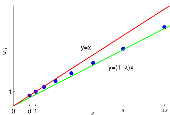
Figure 1. A path of the shadow price process

What happens when $S_{t}$ increases beyond $S_{0}$? Intuitively, it seems clear that we will not change the log-optimal portfolio at times $t$ with $S_{t}>S_{0}$ except by selling stock, i.e., for positive $n$ we expect to have $(1-\lambda)S_{n}\leq\widetilde{S}_{n}<S_{n}$. Thus, during a positive excursion of the stock price process $S$ from $S_{0}$, the excursion of the shadow price process away from the bid-ask price boundary will end at $\tau\coloneqq\min\left\{t\geq 0\ \big{|}\ \widetilde{S}_{t}=(1-\lambda)S_{t}\right\}$, assuming that $\forall 0\leq t\leq\tau:\ S_{t}\geq S_{0}$. We also let $k\coloneqq n(\tau)$ be the corresponding net number of upwards steps. This means that

$$\frac{\varphi^{0}_{n}}{\varphi_{n}S_{0}}=c\text{ for }0\leq n\leq k-1$$

As for $0\leq n\leq k-1$ the numbers of bonds and stock in the log-optimal portfolio for the market given by $\widetilde{S}$ may not change, Proposition 2.1 implies

(1) $$\pi_{n}=\frac{\varphi_{n}\widetilde{S}_{n}}{\varphi^{0}_{n}+\varphi_{n}\widetilde{S}_{n}}=\frac{\widetilde{S}_{n}}{cS_{0}+\widetilde{S}_{n}}=\frac{p\widetilde{u}_{n+1}+(1-p)\widetilde{d}_{n+1}-1}{(\widetilde{u}_{n+1}-1)(1-\widetilde{d}_{n+1})}.$$

where

$$\widetilde{u}_{n+1}=\frac{\widetilde{S}_{n+1}}{\widetilde{S}_{n}}\text{ and }\widetilde{d}_{n+1}=\frac{\widetilde{S}_{n-1}}{\widetilde{S}_{n}}.$$

Solving (1) gives the recursion

$$\widetilde{S}_{n+1}=\frac{\widetilde{S}_{n}cS_{0}+p\widetilde{S}_{n}\widetilde{S}_{n-1}-cS_{0}(1-p)\widetilde{S}_{n-1}}{pcS_{0}+\widetilde{S}_{n-1}-(1-p)\widetilde{S}_{n}},\ \widetilde{S}_{0}=S_{0}\text{ and }\widetilde{S}_{-1}=S_{0}d.$$

Fortunately, we can find an explicit solution for the above recursion. It is given by

(2) $$\widetilde{S}_{n} =S_{0}\frac{c(1-(\frac{1-p}{p})^{n})+\beta_{p}}{-(1-(\frac{1-p}{p})^{n})+\beta_{p}} \mbox{ for }p\neq\frac{1}{2},$$

(3) $$\widetilde{S}_{n} =S_{0}\frac{cn+\beta}{-n+\beta} \mbox{ for }p=\frac{1}{2},$$

where $\beta_{p}=\frac{(c+d)(2p-1)}{(1-d)(1-p)}$ and $\beta=\frac{c+d}{1-d}.$

When we do not want to parametrize the shadow price process in terms of $n$, we can still express $\widetilde{S}_{t}=S_{0}g_{c}(S_{t})$ for $0\leq t\leq\tau$. Indeed, by $S_{n}=S_{0}u^{n}$ we see that we can express $n$ in terms of the stock price $s$ by $n=\frac{\log(s)}{\log(u)}$, and inserting into (2) gives

$$g_{c}(s) =\frac{c\left(1-(\frac{1-p}{p})^{-\frac{\log(s)}{\log d}}\right)+\beta_{p}}{-\left(1-(\frac{1-p}{p})^{-\frac{\log(s)}{\log d}}\right)+\beta_{p}} \mbox{ for }p\neq\frac{1}{2},$$

$$g_{c}(s) =\frac{c\log(s)+\beta\log u}{-\log(s)+\beta\log u} \mbox{ for }p=\frac{1}{2}.$$

Note that $g_{c}(s)$ is increasing, first concave and then convex.

Now we have constructed a candidate for the shadow price process $\widetilde{S}$ which is defined until the first time when it again hits either the bid or the ask price of the true stock. We have also, en passant, settled the case when the process first hits the ask price again: for $n=-1$, we have $\widetilde{S}_{-1}=S_{-1}=dS_{0}$, and we will buy additional stock and re-start the recursion, but at a different initial value, see the next section for a detailed account. However, when we actually consider the passage from ask to bid price, i.e., when $n=k$ and $\widetilde{S}_{k}=(1-\lambda)S_{k}$, we have to decide how to re-balance our portfolio. In practice, the situation will be a bit difficult: most likely, we are not able to follow our explicit formula (2), as it is quite possible that $\widetilde{S}_{k}<(1-\lambda)S_{k}$, i.e., that the recursion formula does not hold true anymore for the last step, because it would induce a violation of the first basic property of the shadow price process. In principle, it would be possible to handle this situation. However, it would lead to inherent non-continuities, which would not allow us to use the method of asymptotic expansions. Thus, we assume that the shadow price process touches the bid price at an integer point $k$. (Note that this is really an assumption on the model parameter, not just an ansatz! The assumption will be made more explicit in Assumption 4.3 in the subsequent section.)

Assumption 3.3.

The model parameters ($u$, $d$, $p$, $S_{0}$ and $\lambda$) are chosen such that $\widetilde{S}_{k}=(1-\lambda)u^{k}S_{0}$ and $\widetilde{S}_{k+1}=(1-\lambda)u^{k+1}S_{0}$.

The second part of Assumption 3.3 requires some justification. In fact, it reflects a choice on the trading involved at the first opportunity of selling. More precisely, it means that we do not re-balance the log-optimal portfolio when the shadow price process first hits the bid price. Only when the stock price increases once more, the shadow price is again equal to the bid price and then we do trade. In the discrete time situation, this particular structure of the shadow price process seems arbitrary, but it reflects an important condition in the continuous problem as discussed in [GMKS11], namely the smooth pasting condition for the analogous function $g$ in the Black-Scholes model with proportional transaction costs. This condition says that $g$ is continuously differentiable at $\overline{s}$ with $g(\overline{s})=(1-\lambda)\overline{s}$, i.e., in some sense the shadow price process “smoothly” merges with the bid price process. In continuous time, this assumption is very beneficial in, for instance, avoiding any reference to local times. In the discrete case, other choices are clearly also possible, which lead, inter alia, to different shadow price processes as the one studied by [GMKS11] in the Black-Scholes model seen as a limiting case of the binomial model. Since one of the main motivations for the present model is to study precisely this convergence, we impose the second part of Assumption 3.3.

In the next step, we interpret the two equalities in Assumption 3.3 as a system of equations for the two unknowns $k$ and $\lambda$. For $p=\frac{1}{2},$ the solution is given by $k=\frac{(c+d)(c-1)}{c(1-d)}$ and $\lambda=1-c^{2}d^{k}.$

For $p\neq\frac{1}{2}$, set $x=\frac{1-p}{p}$ and $y=x^{k}$. If we eliminate $\lambda$ from equations, then we obtain

(4) $$\frac{c(1-y)+\beta_{p}}{-(1-y)+\beta_{p}}=\frac{c(1-xy)+\beta_{p}}{-(1-xy)+\beta_{p}}d$$

which is second order polynomial equation for $y.$ We obtain two solutions $y_{1}$ to be given in (5) and $y_{2}=\frac{p}{1-p}$ which implies that the net number of upwards steps is $k=-1$. However, for $k=-1$, we indeed solve equation (4), but at the ask-price instead of the bid price. Therefore, the remaining solution must be the appropriate one,

(5) $$y=\frac{[c(p+pd-d)+d(2p-1)][1-p-pd-c(2p-1)]}{c(1-d)^{2}(1-p)^{2}}.$$

Hence, $\bar{s}=d^{-k}=y^{-\log(d)/\log(x)}.$ Inserting this, we obtain

(6) $$\lambda=\frac{(cp((c+2)d+c)-c(c+1)d)\left(-\frac{c(d-1)^{2}(p-1)^{2}}{((c+2)dp-(c+1)d+cp)(c(2p-1)+dp+p-1)}\right)^{-\frac{\log(d)}{\log\left(x\right)}}}{c(2p-1)+dp+p-1}+1\eqqcolon F(c).$$

Remark 3.4.

If we are mainly interested in the limit to the Black-Scholes model, we may assume that $u-1\ll\lambda$. In that case, we can anyway bound

$$\left\lvert\widetilde{S}_{\tau}-\widetilde{S}_{\left\lceil\tau\right\rceil}\right\rvert\leq(u-1)\widetilde{S}_{\tau}\ll\lambda\widetilde{S}_{\tau}.$$

Thus, in that sense, it should not matter for the asymptotic result, how we treat the boundary conditions, and whether we really hit at an integer point in time.

4. Formal construction of the shadow price process

The proofs of most propositions in this section are found in Appendix A. From now on we fix $S_{0}=1,0<\lambda<1,$ $1>d=1/u>0$ and $\frac{d}{1+d}<p<\frac{1}{1+d}.$ (The last inequality translates to the condition $0<\mu<\sigma^{2}$ in the Black-Scholes case. By modifying some of the functions, it is also possible to carry out the whole analysis for the other cases.)Moreover, we denote $\bar{c}=\frac{1-p-pd}{p+pd-d}$ and $b=\frac{\log(d)}{\log\left((1-p)/p\right)}.$ Note that the optimal wealth fraction $\pi_{t}$ in the frictionless binomial model is by Proposition 2.1 given by $\pi_{t}=\frac{1}{1+\bar{c}}$.

Proposition 4.1.

Define

$$F(c):=\begin{cases}1-\left(\frac{c(p+pd-d)+d(2p-1)}{(1-d)(1-p)}\right)^{2}\left(\frac{(c(p+pd-d)+d(2p-1))(1-p-pd-c(2p-1))}{c(1-d)^{2}(1-p)^{2}}\right)^{b-1}&\mbox{ for }p\neq\frac{1}{2},\\ 1-c^{2}d^{\frac{(c+d)(c-1)}{c(1-d)}}&\mbox{ for }p=\frac{1}{2}.\end{cases}$$

Then, $F(c)=\lambda$ has a unique solution in $(\bar{c},\infty)$ if $p\in(\frac{d}{1+d},\frac{1}{2}],$ and a unique solution in $(\bar{c},\frac{1-p-pd}{2p-1})$ if $p\in(\frac{1}{2},\frac{1}{1+d}).$

As we have $c,$ we can define $k$ and $\bar{s}.$ Denote

$$r(c)\coloneqq\frac{[c(p+pd-d)+d(2p-1)][1-p-pd-c(2p-1)]}{c(1-d)^{2}(1-p)^{2}}.$$

Proposition 4.2.

Fix $c$ and define

$$k:=\begin{cases}\frac{\log(r(c))}{\log\left(\frac{1-p}{p}\right)}&\mbox{ for }p\neq\frac{1}{2},\\ \frac{(c+d)(c-1)}{c(1-d)}&\mbox{ for }p=\frac{1}{2},\end{cases}$$

and $\bar{s}:=u^{k}.$ We have $k>0.$

Assumption 4.3.

We assume that the model parameter $d$ is given such that $k$ is a positive integer in the above definition.

Note that this is the only assumption left from the previous Section 3. A closer look at the definition of $k$ shows the intuitively obvious fact that $k$ converges to infinity when $d\to 1$. Consequently, at least when we are really interested in binomial models with $d\approx 1$, Assumption 4.3 is easy to fulfill by a slight modification of the model parameters.

Proposition 4.4.

Define the function $g$ on $\{d,1,\ldots,\bar{s},u\bar{s}\}$ by

$$g(s):=\begin{cases}\frac{c\left(1-(\frac{1-p}{p})^{-\frac{\log(s)}{\log d}}\right)+\beta_{p}}{-\left(1-(\frac{1-p}{p})^{-\frac{\log(s)}{\log d}}\right)+\beta_{p}},&\mbox{ for }p\neq\frac{1}{2},\\ \frac{c\log(s)+\beta\log u}{-\log(s)+\beta\log u},&\mbox{ for }p=\frac{1}{2},\end{cases}$$

where $\beta_{p}=\frac{(c+d)(2p-1)}{(1-d)(1-p)}$ and $\beta=\frac{c+d}{1-d}.$ Then $g$ is increasing, maps $\{d,1,\ldots,\bar{s},u\bar{s}\}$ onto $\{d,1,\ldots,(1-\lambda)\bar{s},(1-\lambda)u\bar{s}\}$ and satisfies the “smooth pasting” conditions

(7) $$g(d)=d,\mbox{ }g(1)=1,\mbox{ }g(\bar{s})=(1-\lambda)\bar{s},\mbox{ }g(u\bar{s})=(1-\lambda)u\bar{s}.$$

In addition,

$$(1-\lambda)s\leq g(s)\leq s\mbox{ for }1\leq s\leq\bar{s}.$$

Finally, we have

$$\frac{p\frac{g(us)}{g(s)}+(1-p)\frac{g(ds)}{g(s)}-1}{(\frac{g(us)}{g(s)}-1)(1-\frac{g(ds)}{g(s)})}=\frac{g(s)}{c+g(s)}\mbox{ for }1\leq s\leq\bar{s}.$$

Define the sequence of stopping times $(\varrho_{n})_{n=0}^{\infty}$, $(\sigma_{n})_{n=1}^{\infty}$ and a process $(m_{t})_{t\geq 0}$ by

$$\varrho_{0}=1\mbox{ and }m_{t}=\min_{0\leq i\leq t}S_{i},\mbox{ }0\leq t\leq\sigma_{1},$$

where $\sigma_{1}$ is defined as

$$\sigma_{1}=\min\left\{t\geq\varrho_{0}:\frac{S_{t}}{m_{t}}=\bar{s}\mbox{ }\&\mbox{ }\frac{S_{t-1}}{m_{t-1}}=\bar{s}\right\}.$$

Then, define the process $(M_{t})_{t\geq 0}$ as

$$M_{t}=\max_{\sigma_{1}\leq i\leq t}S_{i},\mbox{ }\sigma_{1}\leq t\leq\varrho_{1},$$

where $\varrho_{1}$ is defined as

$$\varrho_{1}=\min\left\{t\geq\sigma_{1}:\frac{S_{t}}{M_{t}}=\frac{1}{\bar{s}}\mbox{ }\&\mbox{ }\frac{S_{t-1}}{M_{t-1}}=\frac{1}{\bar{s}}\right\}.$$

Afterwards, we again pass to the running minimum and define

$$m_{t}=\min_{\varrho_{1}\leq i\leq t}S_{i},\mbox{ }\varrho_{1}\leq t\leq\sigma_{2},$$

where

$$\sigma_{2}=\min\left\{t\geq\varrho_{1}:\frac{S_{t}}{m_{t}}=\bar{s}\mbox{ }\&\mbox{ }\frac{S_{t-1}}{m_{t-1}}=\bar{s}\right\}.$$

Then, for $t\geq\sigma_{2},$ we define

$$M_{t}=\max_{\sigma_{2}\leq i\leq t}S_{i},\mbox{ }\sigma_{2}\leq t\leq\varrho_{2},$$

where

$$\varrho_{2}=\min\left\{t\geq\sigma_{2}:\frac{S_{t}}{M_{t}}=\frac{1}{\bar{s}}\mbox{ }\&\mbox{ }\frac{S_{t-1}}{M_{t-1}}=\frac{1}{\bar{s}}\right\}.$$

Proceeding in a similar way, we get the stopping times $(\sigma_{n})_{n=1}^{\infty}$, $(\varrho_{n})_{n=1}^{\infty}$. Both $\sigma_{n}$ and $\varrho_{n}$ increase a.s. to infinity. Note that these stopping times are indeed attained because $S$ is a binomial model, $\bar{s}=u^{k}$ where $k\in\mathbb{N}$ and $\frac{S_{0}}{m_{0}}=1,\frac{S_{\sigma_{n}}}{M_{\sigma_{n}}}=1,\frac{S_{\varrho_{n}}}{m_{\varrho_{n}}}=1,\mbox{ for }n\geq 1.$ Moreover, we see that $m_{t}$ and $M_{t}$ are only defined on stochastic intervals $\llbracket\varrho_{n-1},\sigma_{n}\rrbracket$ and $\llbracket\sigma_{n},\varrho_{n}\rrbracket$ respectively. Note that $\bar{s}m_{\sigma_{n}-1}=S_{\sigma_{n}-1}\mbox{ and }M_{\varrho_{n}-1}=\bar{s}S_{\varrho_{n}-1}\mbox{ for }n\geq 1.$ Then, we extend the processes $M$ and $m$ to $\mathbb{N}$ by

$$M_{t}:=\bar{s}m_{t},\mbox{ for }t\in\bigcup_{n=1}^{\infty}\llbracket\varrho_{n-1},\sigma_{n}\llbracket\mbox{ and }m_{t}:=\frac{M_{t}}{\bar{s}},\mbox{ for }t\in\bigcup_{n=1}^{\infty}\llbracket\sigma_{n},\varrho_{n}\llbracket.$$

Therefore, we have

$$m_{t}\leq S_{t}\leq\bar{s}m_{t}\mbox{ for }t\geq 0.$$

Furthermore, by construction, $m$ decreases only on $\{S_{t}=m_{t}\}$ and increases only on $\{S_{t}=M_{t}\}=\{S_{t}=\bar{s}m_{t}\}.$

Now, we can define a candidate for a shadow price. The result shows that it is a generalized binomial model.

Proposition 4.5.

Define $\widetilde{S}_{t}=m_{t}g(\frac{S_{t}}{m_{t}}),t\geq 0.$ Then, $\widetilde{S}$ is an adapted process which lies in the bid-ask interval $[(1-\lambda)S,S].$ Moreover, consider the multipliers $\widetilde{u}_{t}$ and $\widetilde{d}_{t}$ implicitly defined by

$$\widetilde{S}_{t+1}=\begin{cases}\widetilde{u}_{t+1}\widetilde{S}_{t},&S_{t+1}=uS_{t},\\ \widetilde{d}_{t+1}\widetilde{S}_{t},&S_{t+1}=dS_{t},\end{cases}$$

then we have

$$\widetilde{u}_{t+1}=\frac{g(\frac{S_{t}u}{m_{t}})}{g(\frac{S_{t}}{m_{t}})}>1>\widetilde{d}_{t+1}=\frac{g(\frac{S_{t}d}{m_{t}})}{g(\frac{S_{t}}{m_{t}})}.$$

Proof.

$\widetilde{S}$ is adapted because $m$ is adapted. Moreover,

$$1\leq\frac{S_{t}}{m_{t}}\leq\bar{s},\mbox{ for }t\geq 0.$$

Also Proposition 4.4 implies that

$$(1-\lambda)s\leq g(s)\leq s\mbox{ for }1\leq s\leq\bar{s}.$$

Hence $\widetilde{S}$ lies in the bid-ask interval. The ratios in the last assertion easily follow in the case $m_{t}<S_{t}<\bar{s}m_{t}$ as $m_{t}$ does not change. In the cases $S_{t}=m_{t}$ and $S_{t}=\bar{s}m_{t}$ they follow using $g(d)=d$ and $g(u\bar{s})=(1-\lambda)u\bar{s}$ respectively. Finally, $\widetilde{u}_{t+1}>1>\widetilde{d}_{t+1},$ since $g$ is increasing. ∎

The $\log$-optimal portfolio can be given in closed form relative to the process $m$ and the sequence of stopping times $\varrho$ and $\sigma$.

Theorem 4.6.

Let $\widetilde{S}_{t}=m_{t}g\left(\frac{S_{t}}{m_{t}}\right).$ Then the $\log$-optimizer $(\varphi^{0}_{t},\varphi_{t})$ in the frictionless market with $\widetilde{S}$ exists and satisfies $(\varphi^{0}_{-1},\varphi_{-1})=(x,0)$, $(\varphi^{0}_{0},\varphi_{0})=(\frac{cx}{c+1},\frac{x}{c+1})$ and for $t>0$

$$\varphi^{0}_{t}=\begin{cases}\varphi^{0}_{\varrho_{n-1}-1}\left(\frac{c+d}{c+1}\right)^{\frac{\log(m_{t})-\log(m_{\varrho_{n-1}-1})}{\log(d)}},&\mbox{ on }\cup_{n=1}^{\infty}\llbracket\varrho_{n-1},\sigma_{n}\llbracket,\\ \varphi^{0}_{\sigma_{n}-1}\left(\frac{cd+(1-\lambda)\bar{s}}{c+(1-\lambda)\bar{s}}\right)^{\frac{\log(m_{t})-\log(m_{\varrho_{n-1}-1})}{\log(d)}}\frac{m_{t}}{m_{\sigma_{n}}-1},&\mbox{ on }\cup_{n=1}^{\infty}\llbracket\sigma_{n},\varrho_{n}\llbracket,\end{cases}$$

together with

$$\varphi_{t}=\begin{cases}\varphi_{\varrho_{n-1}-1}\left(\frac{c+d}{c+1}\right)^{\frac{\log(m_{t})-\log(m_{\varrho_{n-1}-1})}{\log(d)}}\frac{m_{\varrho_{n-1}-1}}{m_{t}},&\mbox{ on }\cup_{n=1}^{\infty}\llbracket\varrho_{n-1},\sigma_{n}\llbracket,\\ \varphi_{\sigma_{n}-1}\left(\frac{cd+(1-\lambda)\bar{s}}{c+(1-\lambda)\bar{s}}\right)^{\frac{\log(m_{t})-\log(m_{\varrho_{n-1}-1})}{\log(d)}},&\mbox{ on }\cup_{n=1}^{\infty}\llbracket\sigma_{n},\varrho_{n}\llbracket.\end{cases}$$

Furthermore, the optimal fraction of wealth invested in the stock satisfies

$$\widetilde{\pi}_{t}=\frac{\varphi_{t}\widetilde{S}_{t}}{\varphi^{0}_{t}+\varphi_{t}\widetilde{S}_{t}}=\frac{g\left(\frac{S_{t}}{m_{t}}\right)}{c+g\left(\frac{S_{t}}{m_{t}}\right)}.$$

Proof.

We will show that $(\varphi^{0}_{t},\varphi_{t})$ given above is indeed the log-optimal portfolio. It is clear from the above definition that $(\varphi^{0}_{t},\varphi_{t})$ is an adapted process. Inductively, we obtain that

(8) $$\varphi^{0}_{t}=cm_{t}\varphi_{t},\mbox{ for }t\geq 0,$$

both on $\cup_{n=1}^{\infty}\llbracket\varrho_{n-1},\sigma_{n}\llbracket$ and on $\cup_{n=1}^{\infty}\llbracket\sigma_{n},\varrho_{n}\llbracket.$ Therefore, the self-financing condition

$$\varphi^{0}_{t+1}-\varphi^{0}_{t}+\widetilde{S}_{t+1}(\varphi_{t+1}-\varphi_{t})=0,$$

follows easily when $m_{t}$ does not change, as then $\varphi^{0}_{t}$ and $\varphi_{t}$ do not change, either. If $m_{t}$ changes and $t\in\cup_{n=1}^{\infty}\llbracket\varrho_{n-1},\sigma_{n}\llbracket$ , then the self-financing condition follows using (8) and the fact that $\widetilde{S}_{t}=m_{t}\mbox{ and }\widetilde{S}_{t+1}=m_{t+1}=dm_{t}.$ It follows similarly for $t\in\cup_{n=1}^{\infty}\llbracket\sigma_{n},\varrho_{n}\llbracket.$ Therefore, (8) implies that the fraction of wealth in the stock is

$$\frac{\varphi_{t}\widetilde{S}_{t}}{\varphi^{0}_{t}+\varphi_{t}\widetilde{S}_{t}}=\frac{g\left(\frac{S_{t}}{m_{t}}\right)}{c+g\left(\frac{S_{t}}{m_{t}}\right)}.$$

Now, we prove that the same holds for the $\log$-optimizer and hence by uniqueness we are done. By Proposition 4.5, $\widetilde{S}$ is a generalized binomial model and hence Proposition 2.1 and Proposition 4.4 imply that the fraction of wealth invested in the stock is given by

$$\widetilde{\pi}_{t}=\frac{p\widetilde{u}_{t+1}+(1-p)\widetilde{d}_{t+1}-1}{(\widetilde{u}_{t+1}-1)(1-\widetilde{d}_{t+1})}=\frac{p\frac{g(u\frac{S_{t}}{m_{t}})}{g(\frac{S_{t}}{m_{t}})}+(1-p)\frac{g(d\frac{S_{t}}{m_{t}})}{g(\frac{S_{t}}{m_{t}})}-1}{(\frac{g(u\frac{S_{t}}{m_{t}})}{g(\frac{S_{t}}{m_{t}})}-1)(1-\frac{g(d\frac{S_{t}}{m_{t}})}{g(\frac{S_{t}}{m_{t}})})}=\frac{g\left(\frac{S_{t}}{m_{t}}\right)}{c+g\left(\frac{S_{t}}{m_{t}}\right)}.\qed$$

Corollary 4.7.

Let $\widetilde{S}_{t}=m_{t}g\left(\frac{S_{t}}{m_{t}}\right).$ Then $\widetilde{S}_{t}$ is a shadow price.

Proof.

By definition, $m$ decreases only on $\{S_{t}=m_{t}\}$ and increases only on $\{S_{t}=\bar{s}m_{t}\}.$ Hence, by definition of $\varphi$ in Theorem 4.6, we obtain

$$\{\varphi_{t}-\varphi_{t-1}>0\}\subseteq\{S_{t}=m_{t}\}=\{\widetilde{S}_{t}=S_{t}\}\mbox{ and }$$

$$\{\varphi_{t}-\varphi_{t-1}<0\}\subseteq\{S_{t}=\bar{s}m_{t}\}=\{\widetilde{S}_{t}=(1-\lambda)S_{t}\}.\qed$$

5. Asymptotic expansions

Having constructed the shadow price process and the corresponding log-optimal portfolio process in Theorem 4.6, we can now start to reap the benefits. Note, however, that the almost explicit account of the log-optimal portfolio depends on the optimal ratio $c$ between wealth invested in bonds and stocks, respectively. We have implicitly found $c$ as solution of a non-linear equation $\lambda=F(c)$, see (6), but we need a better grip on it to facilitate further understanding of the optimal portfolio under proportional transaction costs $\lambda$, which can be gained by formal series expansions. In the following, denote $\eta\coloneqq\frac{(2p-1)\log(d)}{(1-d)\log((1-p)/p)}$ if $p\neq\frac{1}{2}$ and $\eta\coloneqq\frac{\log(d)}{-2(1-d)}$ if $p=\frac{1}{2}.$

Remark 5.1.

Assuming that we know $c$, we can find the optimal portfolio and the value function by a simple iteration on the tree in forward direction, instead of the typical backward iteration. Thus, the shadow price method can be directly turned into an attractive numerical method by solving the equation for $c$ numerically.

Proposition 5.2.

The optimal ratio of wealth invested in bonds and stocks $c$ has the series expansion

$$c=\bar{c}+\sum_{i=1}^{\infty}c_{i}\lambda^{i},$$

where all the coefficients $c_{i}$ can be computed by means of well-known symbolic algorithms. In particular, the first two coefficients are given by

$$c_{1}=\frac{\bar{c}(1-p)}{(1+d)\eta-1}\mbox{ and }c_{2}=\frac{\bar{c}(1-p)\left[(1+d)^{2}\eta^{2}+\frac{d^{2}+(2-2p)d-1-2p}{1-d}\eta+\frac{2p(p+pd-d)}{1-d}\right]}{2[(1+d)\eta-1]^{3}}.$$

Proof.

We will try to formally invert the power series for $\lambda$ as a function of $c$. Since we can only invert such a power series when the $0$-order term vanishes, we expand the right hand side of equation (6) around the value $c=\overline{c}=\frac{1-p-pd}{p+pd-d}$, which is the optimal $c$ in the frictionless binomial model.

We only consider the case $p\neq\frac{1}{2},$ the case $p=\frac{1}{2}$ being similar. Using Mathematica [Res10], we do a Taylor expansion

(9) $$\lambda=F(c)=\lambda_{1}(c-\overline{c})+\lambda_{2}(c-\overline{c})^{2}+\mathcal{O}((c-\overline{c})^{3}),$$

where

$$\lambda_{1}=\frac{(1+d)\eta-1}{\bar{c}(1-p)},\quad\lambda_{2}=-\frac{(1+d)^{2}\eta^{2}+\frac{d^{2}+(2-2p)d-1-2p}{1-d}\eta+\frac{2p(p+pd-d)}{1-d}}{2\bar{c}^{2}(1-p)^{2}}.$$

Note that all coefficients of the series could, in principle, be found in symbolic form. As the first order term $\lambda_{1}$ does not vanish, the implicit function theorem implies the existence of an analytic local inverse function $F^{-1}$. The power series coefficients of the inverse function can be found using Lagrange’s inversion theorem, see, for instance, [Knu98, p. 527]. Inverting the series (9), we thus obtain obtain a series for $c$ in terms of $\lambda$

(10) $$c=\overline{c}+c_{1}\lambda+c_{2}\lambda^{2}+\mathcal{O}(\lambda^{3}),$$

where

$$c_{1}=\frac{1}{\lambda_{1}}=\frac{\bar{c}(1-p)}{(1+d)\eta-1},c_{2}=-\frac{\lambda_{2}}{\lambda_{1}^{3}}=\frac{\bar{c}(1-p)\left[(1+d)^{2}\eta^{2}+\frac{d^{2}+(2-2p)d-1-2p}{1-d}\eta+\frac{2p(p+pd-d)}{1-d}\right]}{2[(1+d)\eta-1]^{3}}.$$

Again, we note that higher order coefficients can be obtained explicitly using symbolical algorithms. ∎

Remark 5.3.

When $p\geq 1/2$, Proposition 5.2 yields a nice economic interpretation. Indeed, $c_{1}$ is positive and increasing in $d$ and decreasing in $p$. Hence, the investor becomes more conservative in the presence of transaction costs, as $c_{1}\geq 0$, and this is more pronounced when $d$ is large or $p$ is small, as in these cases the potential average gains from investment in the risky asset are relatively small. For $p<1/2$, the situation is less intuitive, as then the optimal fraction $c$ can become negative, and it does so in a singular way – by a jump from $+\infty$ to $-\infty$.

When following the optimal strategy given in Theorem 4.6, the fraction $\pi_{t}$ of the total wealth invested in the stock is kept in the interval $[(1+c)^{-1},(1+c/\overline{s})^{-1}]$, the no-trade region.

Theorem 5.4.

The lower and upper boundaries $\underline{\theta}$ and $\overline{\theta}$ of the no-trade-region satisfy the asymptotic expansions

$$\underline{\theta}\coloneqq\frac{1}{1+c}=\frac{p+pd-d}{1-d}-\frac{(1-p-pd)(p+pd-d)(1-p)}{((1+d)\eta-1)(1-d)^{2}}\lambda+\mathcal{O}(\lambda^{2}),$$

$$\overline{\theta}\coloneqq\frac{1}{1+c/\bar{s}}=\frac{p+pd-d}{1-d}+\frac{(1-p-pd)(p+pd-d)((1+d)\eta-(1-p))}{((1+d)\eta-1)(1-d)^{2}}\lambda+\mathcal{O}(\lambda^{2})$$

for $p\neq 1/2$ and

$$\underline{\theta}\coloneqq\frac{1}{2}-\frac{1}{4}\frac{1-d}{(1+d)\log(d^{-1})-2(1-d)}\lambda+\mathcal{O}(\lambda^{2}),$$

$$\overline{\theta}\coloneqq\frac{1}{2}+\frac{1}{4}\frac{1-d+(1+d)\log(d)}{2(1-d)+(1+d)\log(d)}\lambda+\mathcal{O}(\lambda^{2})$$

for $p=1/2$. The width of the no-trade-region is therefore given by

$$\overline{\theta}-\underline{\theta}=\frac{(1-p-pd)(p+pd-d)(1+d)\eta}{((1+d)\eta-1)(1-d)^{2}}\lambda+\mathcal{O}(\lambda^{2})$$

for $p\neq 1/2$ and similarly for $p=1/2$.

Proof.

We again assume $p\neq\frac{1}{2},$ the case $p=\frac{1}{2}$ being similar. We first need to compute the expansion for $\bar{s}=u^{k}$. Inserting the expansion for $c$ given in Proposition 5.2 into the formula for $\overline{s}$ given in Proposition 4.2, we obtain

$$\bar{s}=1+s_{1}\lambda+\mathcal{O}(\lambda^{2}),$$

where $s_{1}=\frac{(1+d)\eta}{(1+d)\eta-1}$ and the further coefficients can, as usually, be computed using symbolic algorithms. Then, again taking advantage of Mathematica [Res10], we find that the lower boundary and the upper boundaries of the no-trade region have the asymptotic series expansions

$$\underline{\theta}=\frac{1}{1+c}=\frac{p+pd-d}{1-d}-\frac{(1-p)(1-p-pd)(p+pd-d)}{((1+d)\eta-1)(1-d)^{2}}\lambda+\mathcal{O}(\lambda^{2}),$$

$$\overline{\theta}=\frac{1}{1+c/\bar{s}}=\frac{p+pd-d}{1-d}+\frac{(1-p-pd)(p+pd-d)((1+d)\eta-(1-p))}{((1+d)\eta-1)(1-d)^{2}}\lambda+\mathcal{O}(\lambda^{2}).$$

By subtracting, we get the desired formula for the width of the no-trade region. ∎

Remark 5.5.

Note that the width of the no-trade-region is positive and increasing in $d$ to first order. This makes sense economically as larger $d$ means that the returns in the risky asset are smaller, so it makes sense to be more stringent about the transactions costs. Moreover, to first order the width of the no-trade-region is increasing in $p$ for $p<1/2$ and decreasing for $p>1/2$. In other words, the size of the no-trade-regions increases with the “variability” of the stock returns.

Finally, we prove the second part of Corollary 2.7.

Lemma 5.6.

Let $(\varphi^{0},\varphi)$ be the log-optimal portfolio of the shadow-price process. For $\lambda$ small enough we can find a positive, bounded random variable $Y=Y(\lambda)$ having a finite, deterministic limit $Y(0)=\lim_{\lambda\to 0}Y(\lambda)$ such that

$$\sup_{(\psi^{0},\psi)}\mathbb{E}[\log({V}_{T}(\psi^{0},\psi))]+E[\log(1-\lambda Y(\lambda))]\leq\mathbb{E}[\log({V}_{T}(\varphi^{0},\varphi))]\leq\sup_{(\psi^{0},\psi)}\mathbb{E}[\log({V}_{T}(\psi^{0},\psi))].$$

Proof.

It is easy to see that $(1-\xi)\widetilde{V}_{T}(\varphi^{0},\varphi)\leq V_{T}(\varphi^{0},\varphi)$ provided that

$$\xi\geq\lambda\max\left(-\left(1-\lambda+\frac{\varphi^{0}_{T}}{\varphi_{T}S_{t}}\right)^{-1},\ \left(1+\frac{\varphi^{0}_{T}}{\varphi_{T}S_{T}}\right)^{-1}\right)\eqqcolon\lambda Y(\lambda).$$

Boundedness and positivity of $Y$ now follows from Theorem 4.6 above, and we note that the limit for $\lambda\to 0$ is precisely given by the Merton proportion. The rest of the argument works just as for Corollary 2.7. ∎

6. The optimal growth rate

In the following, we are going to consider the optimal growth rate as given in Definition 2.8. In the frictionless binomial model, we recall from the proof of Proposition 2.1 that the value of the log-optimal strategy satisfies $V_{T}=\frac{V_{0}}{Z_{T}}$ and hence the expected utility is given by

$$\mathbb{E}[\log(V_{T})]=\log(V_{0})+T\log\left(\frac{(1+d)p^{p}(1-p)^{1-p}}{d^{p}}\right).$$

Therefore, the optimal growth rate satisfies

(11) $$\lim_{T\to\infty}\frac{\mathbb{E}[\log(V_{T})]}{T}=\log\left(\frac{(1+d)p^{p}(1-p)^{1-p}}{d^{p}}\right).$$

Theorem 6.1.

The optimal growth rate in a binomial model with proportional transaction costs satisfies

$$R=\frac{c(1-d)}{c^{2}-d}\log\left(\frac{(c+d)}{\sqrt{d}(c+1)}\right)$$

when $p=\frac{1}{2}$ and

$$R=\frac{1-2p}{(1-p)(1-(\frac{p}{1-p})^{k+1})}\left[(1-p)\log\left(\frac{c+d}{c+1}\right)+p\left(\frac{p}{1-p}\right)^{k}\log\left(\frac{(c+d)p}{(c-1)(1-p)d}\right)\right]$$

otherwise.

Proof.

We recall from Proposition 4.5 that up and down factors for $\widetilde{S}$ are $\widetilde{u}_{t+1}=\frac{g(Z_{t}u)}{g(Z_{t})}$ and $\widetilde{d}_{t+1}=\frac{g(Z_{t}d)}{g(Z_{t})},$ where $Z_{t}\coloneqq\frac{S_{t}}{m_{t}}.$ Hence, using Proposition 2.1, we compute the expected $\log$-utility as

$$\mathbb{E}[\log(\widetilde{V}_{T})]= \log(\widetilde{V}_{0})-\sum_{t=1}^{T}\mathbb{E}\left[\log\left(\frac{\widetilde{p}_{t}}{p}\mathbf{1}_{\left\{1\right\}}(w_{t})+\frac{\widetilde{q}_{t}}{1-p}\mathbf{1}_{\left\{-1\right\}}(w_{t})\right)\right]$$

$$= \log(\widetilde{V}_{0})-p\sum_{t=1}^{T}\mathbb{E}\left[\log\left(\frac{1-\widetilde{d}_{t}}{p\left(\widetilde{u}_{t}-\widetilde{d}_{t}\right)}\right)\right]-(1-p)\sum_{t=1}^{T}\mathbb{E}\left[\log\left(\frac{\widetilde{u}_{t}-1}{(1-p)\left(\widetilde{u}_{t}-\widetilde{d}_{t}\right)}\right)\right]$$

$$= \log(\widetilde{V}_{0})-p\sum_{t=1}^{T}\mathbb{E}\left[\log\left(\frac{g(Z_{t-1})-g(Z_{t-1}d)}{p\left(g(Z_{t-1}u)-g(Z_{t-1}d)\right)}\right)\right]$$

$$-(1-p)\sum_{t=1}^{T}\mathbb{E}\left[\log\left(\frac{g(Z_{t-1}u)-g(Z_{t-1})}{(1-p)\left(g(Z_{t-1}u)-g(Z_{t-1}d)\right)}\right)\right].$$

Now, we know from Proposition 4.4 that $\frac{pg(us)+(1-p)g(ds)-1}{(g(us)-g(s))(g(s)-g(ds))}=\frac{1}{c+g(s)}\mbox{ for }1\leq s\leq\bar{s}.$ Then, an elementary calculation implies

$$\frac{g(s)-g(ds)}{p(g(us)-g(ds))}=\frac{c+g(s)}{c+g(us)},\quad\frac{g(us)-g(s)}{(1-p)(g(us)-g(ds))}=\frac{c+g(s)}{c+g(ds)}.$$

Thus, using these identities we obtain that

$$R =\lim_{T\to\infty}\left\{-p\frac{1}{T}\sum_{t=1}^{T}\mathbb{E}\left[\log\left(\frac{c+g(Z_{t-1})}{c+g(Z_{t-1}u)}\right)\right]-(1-p)\frac{1}{T}\sum_{t=1}^{T}\mathbb{E}\left[\log\left(\frac{c+g(Z_{t-1})}{c+g(Z_{t-1}d)}\right)\right]\right\}$$

$$=-p\mathbb{E}^{*}\left[\log\left(\frac{c+g(Z_{t})}{c+g(uZ_{t})}\right)\right]-(1-p)\mathbb{E}^{*}\left[\log\left(\frac{c+g(Z_{t})}{c+g(dZ_{t})}\right)\right],$$

where the last step is due to the ergodic theorem and $\mathbb{E}^{*}$ denotes the expectation with respect to the invariant distribution of $Z_{t}$. Note that $Z_{t}$ is a Markov chain with state space $\{1,u,u^{2},\ldots,u^{k}\}$ and transition matrix

$$P_{i,j}\coloneqq\mathbb{P}[Z_{t+1}=u^{j}|Z_{t}=u^{i}]=\begin{cases}p,&j=i+1,\ 0\leq i\leq k-1,\\ 1-p,&j=i-1,\ 1\leq i\leq k,\\ p,&j=i=k,\\ 1-p,&j=i=0,\\ 0,&\mbox{ else. }\end{cases}$$

Then the invariant distribution is the solution of $\alpha^{T}P=\alpha^{T}$ normalized to $\sum_{n}\alpha_{n}=1$. If $p=\frac{1}{2},$ the solution satisfies $\alpha_{n}=\frac{1}{k+1},\mbox{ for }0\leq n\leq k.$ If $p\neq\frac{1}{2},$ we get $\alpha_{n}=\frac{1-2p}{(1-p)\left(1-\left(\frac{p}{1-p}\right)^{k+1}\right)}\left(\frac{p}{1-p}\right)^{n},\mbox{ for }0\leq n\leq k.$

For the remainder of the proof, we assume $p\neq\frac{1}{2},$ the other case being similar. Then, the optimal growth rate becomes

$$R= -p\mathbb{E}^{*}\left[\log\left(\frac{c+g(Z_{t})}{c+g(uZ_{t})}\right)\right]-(1-p)\mathbb{E}^{*}\left[\log\left(\frac{c+g(Z_{t})}{c+g(dZ_{t})}\right)\right]$$

$$= \mathbb{E}^{*}\left[\log\left(-\left(1-(\frac{1-p}{p})^{\frac{\log(Z_{t})}{\log(u)}}\right)+\beta_{p}\right)\right]-p\mathbb{E}^{*}\left[\log\left(-\left(1-(\frac{1-p}{p})^{\frac{\log(uZ_{t})}{\log(u)}}\right)+\beta_{p}\right)\right]$$

$$-(1-p)\mathbb{E}^{*}\left[\log\left(-\left(1-(\frac{1-p}{p})^{\frac{\log(dZ_{t})}{\log(u)}}\right)+\beta_{p}\right)\right]$$

$$= \frac{1-2p}{(1-p)(1-(\frac{p}{1-p})^{k+1})}\Bigg{[}(1-p)\left(\log(\beta_{p})-\log\left(\left(\frac{1-p}{p}\right)^{-1}+\beta_{p}-1\right)\right)$$

$$+p\left(\frac{p}{1-p}\right)^{k}\left(\log\left(\left(\frac{1-p}{p}\right)^{k}+\beta_{p}-1\right)-\log\left(\left(\frac{1-p}{p}\right)^{k+1}+\beta_{p}-1\right)\right)\Bigg{]}$$

$$= \frac{1-2p}{(1-p)(1-(\frac{p}{1-p})^{k+1})}\left[(1-p)\log\left(\frac{c+d}{c+1}\right)+p\left(\frac{p}{1-p}\right)^{k}\log\left(\frac{(c+d)p}{(c-1)(1-p)d}\right)\right].\qed$$

Writing $k$ in terms of $c$ and plugging in the series expansion for $c$, we get

Corollary 6.2.

The optimal growth rate has the expansion

$$R= \log\left(\frac{(1+d)p^{p}(1-p)^{1-p}}{d^{p}}\right)$$

$$+\frac{(p+pd-d)(1-p-pd)-(1+d)^{2}(1-p)p\log\left(\frac{(1+d)^{2}(1-p)p}{d}\right)}{(1-d^{2})\left[(1+d)\eta-1\right]}\lambda+\mathcal{O}(\lambda^{2}).$$

Remark 6.3.

The first order correction term in Corollary 6.2 is negative, reflecting the trivial observation that transaction costs reduce the optimal growth rate. Moreover, contrary to the width of the no-trade-region, the term is decreasing in $d$ and increasing in $p$ for $p>1/2$ and decreasing for $p<1/2$. Thus, the optimal growth rate is most effected by transactions costs, when the model is close to the Black-Scholes model.

7. Convergence to the Black-Scholes model

Historically, proportional transaction costs have mainly been studied in the framework of the Black-Scholes model, see [TKA88], [DN90], [DL91], [SS94], [CK96], [JS04], [KMK10], [GMKS11]. In order to compare our results to previous results, we shall, therefore, obtain a common ground for the binomial model and the Black-Scholes model. When we add more and more periods to the binomial model while letting $u$ and $d$ approach $1$, the binomial model will clearly converge to the Black-Scholes model. Here, we want to keep the convenient choice $d=1/u$, while still allowing all possible drift and volatility values $\mu$ and $\sigma$ in the limiting Black-Scholes model. Hence, we need $p$ converging to $\frac{1}{2}$, but allowing it to be different from $\frac{1}{2}$ for every finite time-step. More precisely, if we choose a time-step $\delta\coloneqq T/N>0$, and define

(12) $$p\coloneqq\frac{1}{2}+\frac{\mu-\frac{\sigma^{2}}{2}}{2\sigma}\sqrt{\delta},\quad d\coloneqq\exp(-\sigma\sqrt{\delta}),$$

$u=1/d$, then the binomial model $(S_{n})_{n=0}^{N}$ with parameters $S_{0}>0$ and $p,u,d$ as above will converge to the geometrical Brownian motion $\left(S_{0}\exp\left(\sigma B_{t}+\left(\mu-\frac{1}{2}\sigma^{2}\right)t\right)\right)_{t\in[0,T]}$ as $N\to\infty$ in distribution – this is a consequence of the invariance principle, see, e.g., Ethier and Kurtz [EK86, Th. 7.4.1]. Moreover, the shadow price process $\widetilde{S}$ of the binomial model with proportional transaction costs $\lambda$ will also converge to the shadow price process of the Black-Scholes model with proportional transaction costs $\lambda$. Indeed, both shadow price processes are parametrized by the respective functions $g_{c}$, in the binomial case given in Proposition 4.4, in the Black-Scholes case given in [GMKS11, Lemma 4.3] as

$$g^{(BS)}_{c}(s)=\begin{cases}\frac{-cs+(2\theta-1+2c\theta)s^{2\theta}}{s-(2-2\theta-c(2\theta-1))s^{2\theta}},&\theta\notin\left\{\frac{1}{2},1\right\},\\ \frac{(c+1)+c\log(s)}{c+1-\log(s)},&\theta=\frac{1}{2},\end{cases}$$

where $\theta\coloneqq\frac{\mu}{\sigma^{2}}$, and it is an easy exercise to verify that

$$\lim_{\delta\to 0}g_{c}(s)=g_{c}^{(BS)}(s).$$

From equation (9) we can, however, see a big difference between the binomial and the Black-Scholes case: In the binomial model, the inverse function theorem shows that we can invert the function $F(c)$ and the inverse function $c=G(\lambda)\coloneqq F^{-1}(\lambda)$ is analytic in a neighborhood of $\lambda=0$. On the other hand, we cannot directly apply the inverse function theorem in the Black-Scholes case, since then the first and second derivatives of $F$ at the corresponding point $\overline{c}=\frac{1-\theta}{\theta}$ vanish. Indeed, this can be seen already from the derivatives in the binomial model. If we plug in (12) and do a Taylor expansion in $\delta$, then the first three derivatives of $F$ are

(13a) $$\lambda_{1}=\frac{2}{3}\theta^{2}\sigma^{2}\delta+\mathcal{O}\left(\delta^{3/2}\right),$$

(13b) $$\lambda_{2}=\frac{2\theta^{3}\sigma}{1-\theta}\sqrt{\delta}+\mathcal{O}\left(\delta\right),$$

(13c) $$\lambda_{3}=\frac{4\theta^{4}}{3\left(\theta-1\right)^{2}}+O\left(\delta^{1/2}\right).$$

In [GMKS11], this problem is solved by taking the third root, i.e., by considering the equation $\lambda^{1/3}=F(c)^{1/3}$. The power series of $F^{1/3}$ around $c=\overline{c}$ – corresponding to $\lambda=0$ – then has non-vanishing first-order term, and thus can be inverted, giving an expansion of $c$ in terms of $\lambda^{1/3}$, see [GMKS11, Proposition 6.1]. In Section 5, we have already discussed the economic implications of this observation.

As a trivial mathematical consequence, we cannot directly obtain the series coefficients of the relevant quantities in the Black-Scholes model as limits of the corresponding series coefficients in the binomial model, as the former are coefficients of a fractional power series in terms of $\lambda^{1/3}$, whereas the latter are coefficients of an ordinary power series in $\lambda$. Indeed, it is easy to see that the power series coefficients of, for instance, $c$ in terms of $\lambda$ in the binomial model diverge when we take the limit $\delta\to 0$, which is owed to the fact that the limiting function is not analytic in $\lambda$ and, hence, does not admit a power series expansion.

On the other hand, we would like to stress that the quantities of interest will actually converge to the corresponding quantities in the Black-Scholes model when $\delta\to 0$. More precisely, let us consider the optimal wealth-fraction $c$ itself. Assuming the parameters (12) in the binomial model with fixed $\mu$ and $\sigma$, let us denote $c\eqqcolon G(\delta,\lambda)$ when we stress the dependence on the remaining variables $\delta>0$ and $\lambda$. Moreover, we denote by $G(0,\lambda)$ the optimal wealth fraction $c$ in the Black-Scholes model with corresponding parameters $\mu$ and $\sigma$. Then we obtain the

Lemma 7.1.

The function $G=G(\delta,\lambda)$ is continuous in its arguments.

For the proof we again refer to Appendix A. To summarize, the actual quantities of interest, like the form and size of the no-trade-region, do converge when we approach the Black-Scholes model by a sequence of binomial models, but their series expansions fail to converge due to non-analyticity of the optimal wealth fraction $c$ at $\delta=0$. Consequently, our methods cannot predict the results in the Black-Scholes model from the corresponding results in the binomial model.

This also implies that one has to be very careful in deriving quantitative information from the series expansions obtained in Sections 5 and 6.2. Indeed, to get quantitative results, one needs to truncate the power series. Unfortunately, for fixed $\lambda$, one needs to include more and more terms of the expansion to get a similar accuracy when $\delta$ becomes smaller.

We can, however, consider the optimal wealth proportion $\overline{c}$ itself. In the asymptotic regime (12), we have

$$\overline{c}=\frac{1-\theta}{\theta}+\frac{\sigma^{2}\left(1-2\theta\right)}{24\theta^{2}}\delta+\frac{\left(24\theta^{2}-22\theta+5\right)\sigma^{4}}{2880\theta^{3}}\delta^{2}+\mathcal{O}\left(\delta^{3}\right),$$

implying that the optimal proportion $\overline{c}$ is larger than the optimal proportion $\overline{c}=\frac{1-\theta}{\theta}$ in the Black Scholes case if and only if $\theta<\frac{1}{2}$.

8. A series expansion when approaching the Black-Scholes model

In Section 5 we have obtained series expansions for the log-optimal ratios of wealth invested in the bond and wealth invested in the stock in terms of the proportional transaction costs $\lambda$, which was valid for “moderate” parameters $p,d,u$ in as much as the coefficients diverge when $d\to 1$. Hence, these formulas are not helpful when considering the asymptotics of the binomial model to the Black-Scholes model, see Section 7 above.

One possible way to obtain the series expansion of quantities of interest in the Black-Scholes model from the related quantities in the binomial model could be a transformation of $F$, in the sense that we could try to find a mollification $\lambda(\delta)$ for $\lambda$ such that $\lambda(0)=\lambda^{1/3}$ and $G=G(\delta,\lambda(\delta))$ is analytic even at $\delta=0$, but we were not successful in finding such mollification. However, it turns out that a much simpler approach can be used to link the asymptotic expansions for the Black-Scholes model and for the binomial model.

Recall that the asymptotic expansion (9) for $F(\delta,c)$ was of the form

$$F(\delta,c)=\sum_{i=1}^{\infty}\lambda_{i}(\delta)(c-\overline{c})^{i}$$

with $\lim_{\delta\to 0}\lambda_{1}(\delta)=\lim_{\delta\to 0}\lambda_{2}(\delta)=0$, but non-trivial limits for $\lambda_{i}(\delta)$, $i\geq 3$, cf. (13). Thus, for $\delta\ll 1$, we may disregard the first two terms and instead consider

$$F_{2}(\delta,c)\coloneqq F(\delta,c)-\lambda_{1}(c-\overline{c})-\lambda_{2}(c-\overline{c})^{2},$$

cf. (9). By (13a) and (13b) we see that $F(\delta,c)=F_{2}(\delta,c)+g(\delta,c)\sqrt{\delta}$ for some function $g$ with non-trivial limit for $\delta\to 0$. As before, denote the inverse function of $F(\delta,c)$ by $G(\delta,\lambda)$ and denote the inverse function of $F_{2}(\delta,c)$ by $G_{2}(\delta,c)$, i.e.,

$$\lambda=F(\delta,G(\delta,\lambda))=F_{2}(\delta,G_{2}(\delta,\lambda)).$$

Lemma 8.1.

We have $G(\delta,\lambda)=G_{2}(\delta,\lambda)+\mathcal{O}(\delta^{1/6}+\lambda)$ for $\delta,\ \lambda\to 0$, uniformly for $\delta\to 0$ in $\lambda$ around $\lambda=0$.

Proof.

By Taylor’s theorem with Lagrange remainder term, we have

$$F_{2}(\delta,G_{2}(\delta,\lambda))-F_{2}(\delta,G(\delta,\lambda)) =\sum_{j=1}^{2}\frac{1}{j!}F_{2}^{(j)}(\delta,G(\delta,\lambda))(G_{2}(\delta,\lambda)-G(\delta,\lambda))^{j}+$$

$$\quad+\frac{1}{6}F_{2}^{(3)}(\delta,\xi)(G_{2}(\delta,\lambda)-G(\delta,\lambda))^{3}$$

for some $\xi=\xi(\delta,\lambda)$ between $G(\delta,\lambda)$ and $G_{2}(\delta,\lambda)$. At this point, let us note that $G_{2}(\delta,\lambda)-G(\delta,\lambda)$ is bounded in a neighborhood of $(0,0)$ by continuity. Since

$$G(\delta,\lambda)=\overline{c}+\frac{\overline{c}(1-p)}{(1+d)\eta-1}\lambda+\mathcal{O}(\lambda^{2}),$$

we get

$$F_{2}^{\prime}(\delta,G(\delta,\lambda)) =3\lambda_{3}(\delta)\left(G(\delta,\lambda)-\overline{c}\right)^{2}+\mathcal{O}\left(\left(G(\delta,\lambda)-\overline{c}\right)^{3}\right)$$

$$=3\lambda_{3}(\delta)\frac{\overline{c}^{2}(1-p)^{2}}{\left((1+d)\eta-1\right)^{2}}\lambda^{2}+\mathcal{O}\left(\lambda^{3}\right),$$

$$F_{2}^{\prime\prime}(\delta,G(\delta,\lambda)) =6\lambda_{3}(\delta)\left(G(\delta,\lambda)-\overline{c}\right)+\mathcal{O}\left(\left(G(\delta,\lambda)-\overline{c}\right)^{2}\right)$$

$$=6\lambda_{3}(\delta)\frac{\overline{c}(1-p)}{(1+d)\eta-1}\lambda+\mathcal{O}\left(\lambda^{2}\right).$$

On the other hand, we also have

$$F_{2}(\delta,G_{2}(\delta,\lambda))-F_{2}(\delta,G(\delta,\lambda)) =F_{2}(\delta,G_{2}(\delta,\lambda))-(F(\delta,G(\delta,\lambda))-g(\delta,G(\delta,\lambda))\sqrt{\delta})$$

$$=g(\delta,G(\delta,\lambda))\sqrt{\delta}.$$

Consequently, we get

$$\left(G_{2}(\delta,\lambda)-G(\delta,\lambda)\right)^{3} =\frac{6}{F_{2}^{(3)}(\delta,G(\delta,\xi(\delta,\lambda)))}\Bigl{[}g(\delta,G(\delta,\lambda))\sqrt{\delta}+$$

$$\quad+3\lambda_{3}(\delta)\frac{\overline{c}^{2}(1-p)^{2}}{\left((1+d)\eta-1\right)^{2}}\lambda^{2}\left(G_{2}(\delta,\lambda)-G(\delta,\lambda)\right)+\mathcal{O}\left(\lambda^{3}\right)+$$

$$\quad+3\lambda_{3}(\delta)\frac{\overline{c}(1-p)}{(1+d)\eta-1}\lambda\left(G_{2}(\delta,\lambda)-G(\delta,\lambda)\right)^{2}+\mathcal{O}\left(\lambda^{2}\right)\Bigr{]}.$$

When the $\sqrt{\delta}$-term is dominating in the right hand side, then this implies that $G(\delta,\lambda)=G_{2}(\delta,\lambda)+\mathcal{O}(\delta^{1/6})$. In the other two possible cases, we get $G(\delta,\lambda)=G_{2}(\delta,\lambda)+\mathcal{O}(\lambda)$, implying in total $G(\delta,\lambda)=G_{2}(\delta,\lambda)+\mathcal{O}(\delta^{1/6}+\lambda)$.

Regarding the uniformity in $\lambda$, note that $F_{2}^{(3)}(\delta,G(\delta,\xi(\delta,\lambda))$ is bounded for $0\leq\delta\leq\delta_{0}$ and $0\leq\lambda\leq\lambda_{0}$ and $g(\delta,G(\delta,\lambda))$ converges to some finite, non-zero value. ∎

By construction, we will obtain an asymptotic expansion of the form

$$G_{2}(\delta,\lambda)\approx\sum_{i=1}^{\infty}b_{i}(\delta)\lambda^{i/3}\approx G(\delta,\lambda)+\mathcal{O}(\delta^{1/6}+\lambda).$$

So, the coefficients $b_{1}(\delta)$ and $b_{2}(\delta)$ of $G_{2}$ will be asymptotically (for $\delta\to 0$) equal to the corresponding coefficients of $G(0,\lambda)$. In particular, if we only want to match the first coefficient $b_{1}$, we have to choose $\delta\ll\lambda^{2}$.

This approach allows us to compare the results of the binomial model with the results of the Black-Scholes model, at least provided that $\delta$ is small enough when compared with $\lambda$. Let us exemplify the procedure for the boundaries and the size of the no-trade-regions, which have been calculated in Theorem 5.4 for the binomial model and in [GMKS11, Corollary 6.2] for the Black-Scholes model. For the asymptotics of the optimal growth, we need to consider $\frac{R}{\delta}$ instead of $R$, as the calender time is given in terms of the number of periods $T$ in the binomial model by $T\delta$. We have

Theorem 8.2.

Consider a family of binomial model with parameters $p$ and $d$ given by (12) for fixed $\mu$, $\sigma>0$, $u=1/d$ and proportional transaction costs $\lambda$, which we assume to be small but much larger than $\delta$, at least $\lambda^{2}\gg\delta$. The lower and upper boundaries of the no-trade-region satisfy $\underline{\theta}=\underline{\theta}_{0}+\underline{\theta}_{1}\lambda^{\frac{1}{3}}+\mathcal{O}\left(\lambda^{2/3}\right)$ and $\overline{\theta}=\overline{\theta}_{0}+\overline{\theta}_{1}\lambda^{\frac{1}{3}}+\mathcal{O}\left(\lambda^{2/3}\right)$, respectively, with

$$\underline{\theta}_{0}=\theta+\frac{\sigma^{2}}{24}(2\theta-1)\delta+\mathcal{O}\left(\delta^{3/2}\right),$$

$$\underline{\theta}_{1}=-\left(\frac{3\theta^{2}(1-\theta)^{2}}{4}\right)^{\frac{1}{3}}+\left(\frac{3\theta^{2}(1-\theta)^{2}}{32}\right)^{\frac{1}{3}}(4\theta-3)\sigma\delta^{\frac{1}{2}}+\mathcal{O}\left(\delta\right),$$

$$\overline{\theta}_{0}=\theta+\frac{\sigma^{2}}{24}(2\theta-1)\delta+\mathcal{O}\left(\delta^{3/2}\right),$$

$$\overline{\theta}_{1}=\left(\frac{3\theta^{2}(1-\theta)^{2}}{4}\right)^{\frac{1}{3}}+\left(\frac{3\theta^{2}(1-\theta)^{2}}{32}\right)^{\frac{1}{3}}\sigma\delta^{\frac{1}{2}}+\mathcal{O}\left(\delta\right).$$

Moreover, the width $\overline{\theta}-\underline{\theta}$ of the no-trade-region is given by

$$\left(6\theta^{2}(1-\theta)^{2}\right)^{\frac{1}{3}}\left(1+(1-\theta)\sigma\delta^{\frac{1}{2}}+\mathcal{O}\left(\delta\right)\right)\lambda^{\frac{1}{3}}+\mathcal{O}\left(\lambda^{2/3}\right).$$

The asymptotic optimal growth rate satisfies $\frac{R}{\delta}=R_{0}+R_{1}\lambda^{\frac{1}{3}}+\mathcal{O}\left(\lambda^{2/3}\right),$ where

$$R_{0}=\frac{\mu^{2}}{2\sigma^{2}}+\frac{\sigma^{2}}{24}\theta(\theta-1)(2\theta^{2}-2\theta+1)\delta+\mathcal{O}\left(\delta^{3/2}\right),$$

$$R_{1}=\left(\frac{3}{32}\right)^{\frac{1}{3}}\sigma^{3}(\theta(\theta-1))^{\frac{5}{3}}\delta^{1/2}+\mathcal{O}\left(\delta\right).$$

Note that in all of the above terms, the zero-order term in $\delta$ is equal to the corresponding term in the Black-Scholes model, which again justifies our approach. Interestingly, lowest order effect of discrete time seems to be a shift of the no-trade region. The zero-order terms of both $\underline{\theta}$ and $\overline{\theta}$ in the binomial model only differ from the corresponding terms in the Black-Scholes model by the term $\frac{\sigma^{2}}{24}(2\theta-1)$, i.e., the no-trade-region is simply shifted by that term, which is positive when $\theta>\frac{1}{2}$ and negative when $\theta<\frac{1}{2}$. Consequently, the size of the no-trade-region is not effected by discrete time at lowest order. At order $\lambda^{1/3}$, however, the width of the no-trade region in the binomial model is larger than the size of the no-trade-region in the binomial model by the term $6\theta^{2}(1-\theta)^{2}(1-\theta)\sigma\sqrt{\delta}\lambda^{1/3}$ plus higher order term. This observation seems to be counter-intuitive, as the time-discreteness should actually lead to a smaller no-trade-region, as an infinite variation of trading can anyway not be accumulated since there are only finitely many possible trading times – which is also reflected by the results when we do not consider $\delta\to 0$. This indicates that the truncation $F\mapsto F_{2}$ over-compensates for the effects of continuous-time-trading.

Proof of Theorem 8.2.

Define $\tilde{\lambda}=\lambda-\lambda_{1}(c-\bar{c})-\lambda_{2}(c-\bar{c})^{2}.$ Then,

$$\tilde{\lambda}=\lambda_{3}(c-\bar{c})^{3}+\lambda_{4}(c-\bar{c})^{4}+\lambda_{5}(c-\bar{c})^{5}+\mathcal{O}((c-\bar{c})^{6})).$$

Inverting the series using Lagrange’s theorem, we obtain

$$c=\bar{c}+(\frac{1}{\lambda_{3}})^{\frac{1}{3}}\tilde{\lambda}^{\frac{1}{3}}-\frac{1}{3}\left(\left(\frac{1}{\lambda_{3}}\right){}^{5/3}\lambda_{4}\right)\tilde{\lambda}^{2/3}+\frac{\left(\lambda_{4}^{2}-\lambda_{3}\lambda_{5}\right)\tilde{\lambda}}{3\lambda_{3}^{3}}+\mathcal{O}\left(\tilde{\lambda}^{4/3}\right)$$

valid when $\delta$ is small enough as compared to $\lambda$. $\bar{c}$ was already computed in the previous section and is given by

$$\bar{c}=\frac{1-\theta}{\theta}+\frac{\sigma^{2}\left(1-2\theta\right)}{24\theta^{2}}\delta+\frac{\left(24\theta^{2}-22\theta+5\right)\sigma^{4}}{2880\theta^{3}}\delta^{2}+\mathcal{O}\left(\delta^{3}\right).$$

Asymptotics for two more coefficients are given by

$$\tilde{c}_{3}=\frac{1-\theta}{2\theta}\left(\frac{6}{\theta(1-\theta)}\right)^{\frac{1}{3}}+\mathcal{O}(\delta^{\frac{1}{2}}),$$

$$\tilde{c}_{4}=\frac{(1-\theta)^{2}}{4\theta}\left(\frac{6}{\theta(1-\theta)}\right)^{\frac{2}{3}}+\mathcal{O}(\delta^{\frac{1}{2}}).$$

As $\bar{s}$ is a function of $c$, after plugging, we get

$$\bar{s}=1+\bar{s}_{1}\lambda^{\frac{1}{3}}+\bar{s}_{2}\lambda^{\frac{2}{3}}+\bar{s}_{3}\lambda+\mathcal{O}\left(\lambda\right),$$

where asymptotics are given by

$$\bar{s}_{1}=\left(\frac{6}{\theta(1-\theta)}\right)^{\frac{1}{3}}+\left(\frac{6(1-\theta)^{2}}{\theta}\right)^{\frac{1}{3}}\sigma\delta^{\frac{1}{2}}+\mathcal{O}(\delta).$$

$$\bar{s}_{2}=\frac{1}{2}\left(\frac{6}{\theta(1-\theta)}\right)^{\frac{2}{3}}+\frac{(7-2\theta)(1-\theta)\sigma}{4}\left(\frac{6}{\theta(1-\theta)}\right)^{\frac{2}{3}}\delta^{\frac{1}{2}}+\mathcal{O}(\delta).$$

From here on, we just need to follow the proof of Theorem 5.4 and Theorem 6.1, respectively, using the new asymptotics derived above for $c$ and $\overline{s}$. ∎

Appendix A Proofs of Some Theorems

Proof of Proposition 4.1.

For $p=\frac{1}{2},$ we have $\bar{c}=1$ and $F(\bar{c})=F(1)=0.$ Moreover,

$$F^{\prime}(c)=-\frac{\log(d)}{1-d}d^{\frac{(c+d)(c-1)}{c(1-d)}}\left[c^{2}+d+2\frac{1-d}{\log(d)}c\right].$$

We see that $F$ is increasing on $[x_{1},\infty)$ where $x_{1}=\frac{1-d}{-\log(d)}+\sqrt{(\frac{1-d}{-\log(d)})^{2}-d}$ is the larger root of the parabola $c^{2}+d+2\frac{1-d}{\log(d)}c.$ Elementary calculus shows that $1>x_{2}.$ Hence, we conclude that there exists a unique $c>1$ s.t. $F(c)=\lambda.$

Now, let $p\neq\frac{1}{2}$. Denote $c_{1}=\frac{d(1-2p)}{p+pd-d}$ and $c_{2}=\frac{1-p-pd}{2p-1}$ which are the roots of $c(p+pd-d)+d(2p-1)$ and $1-p-dp-c(2p-1),$ respectively. Moreover, denote

(14) $$r(c)=\frac{[c(p-d+pd)+d(2p-1)][1-p-dp-c(2p-1)]}{c(1-d)^{2}(1-p)^{2}}.$$

We see that $F(\bar{c})=0$ and

$$F^{\prime}(c) =(2p-1)(p+pd-d)\Bigg{(}\frac{c^{2}(1+b)-2c_{2}c+(b-1)d\bar{c}}{\big{[}1-p-dp-c(2p-1)\big{]}^{2}}\Bigg{)}r(c)^{b}.$$

If $\frac{1}{2}<p<\frac{1}{1+d},$ then $c_{1}<0<\bar{c}<c_{2}$ and $b>1.$ Note that $r(c)>0$ for $\bar{c}<c<c_{2}$ and $r(c)\to 0$ for $c\uparrow c_{2}.$ Hence, we obtain $F(c)\to 1\mbox{ for }c\uparrow c_{2}.$ Intermediate value theorem implies that there is a $c$ on $(\bar{c},c_{2}).$ s.t. $F(c)=\lambda.$

We see that if $\bar{c}<c<c_{2},$ then the sign of the parabola $c^{2}(1+b)-2c_{2}c+(b-1)d\bar{c}$ determines the sign of $F^{\prime}.$ If the parabola has no root, then $F^{\prime}(c)>0$ for $\bar{c}<c<c_{2}.$ Recalling $F(\bar{c})=0,$ we conclude that there exists a unique $c$ on $(\bar{c},c_{2})$ s.t. $F(c)=\lambda.$ If the parabola has a root, then the smaller root $x_{1}$ satisfies

$$x_{1}\leq\frac{c_{2}}{1+b}<\frac{c_{2}}{c_{2}+2}\leq\bar{c}.$$

Hence, depending on whether $\bar{c}<x_{2}$ or not, $F$ decreases on $(\bar{c},x_{2})$ and increases on $(x_{2},c_{2})$ or only increases on $(\bar{c},c_{2}).$ Due to $F(\bar{c})=0,$ in both cases, we get that there exists a unique $c$ on $(\bar{c},c_{2})$ s.t. $F(c)=\lambda.$

If $\frac{d}{1+d}<p<\frac{1}{2},$ then $c_{2}<0<c_{1}<\bar{c}$ and $b<-1.$ Note that $r(c)>0$ for $c>\bar{c}$ and

$$\frac{r(c)}{\frac{c(p+pd-d)+d(2p-1)}{(1-d)(1-p)}}\to\frac{1-2p}{(1-d)(1-p)}>0\mbox{ for }c\uparrow\infty.$$

Since $b-1<-2,$ we get $F(c)\to 1\mbox{ for }c\uparrow\infty.$ Now, intermediate value theorem implies that there is a $c\in(\bar{c},\infty)$ s.t. $F(c)=\lambda.$

If $c>\bar{c},$ then the sign of $F^{\prime}$ is the opposite of the sign of the parabola $c^{2}(1+b)-2c_{2}c+(b-1)d\bar{c}$ due to $2p-1<0.$ The leading coefficient of the parabola, $1+b,$ is negative. Hence, if the parabola has no root, then $F^{\prime}(c)>0$ for $c>\bar{c}.$ Hence, there exists a unique $c$ on $(\bar{c},\infty)$ s.t. $F(c)=\lambda.$ If the parabola has a root, then the smaller root $x_{1}$ satisfies

$$x_{1}\leq\frac{c_{2}}{1+b}\leq\bar{c},$$

where the last inequality follows due to the fact that the function $w(z)=\frac{z\log(z)}{z-1}$ is increasing on $(1,\infty)$ and hence $w(\frac{1-p}{p})\leq w(u).$ Hence, by the same argument as in the previous case, we obtain that there exist a unique root on $(\bar{c},\infty).$ ∎

Proof of Proposition 4.2.

For $p=\frac{1}{2},$ we know from Proposition 4.1 that $c>1.$ As $\frac{(c+d)(c-1)}{c(1-d)}$ is strictly increasing for $c>0,$ we get $k>0.$

Now let $p\neq\frac{1}{2}.$ Recall, how we defined $r(c).$ Differentiation yields

$$r^{\prime}(c)=\frac{(1-2p)}{(1-d)^{2}(1-p)^{2}}\frac{(p+pd-d)c^{2}+d(1-p-pd)}{c^{2}}.$$

If $\frac{1}{2}<p<\frac{1}{1+d},$ then $c_{1}<0<\bar{c}<c<c_{2}.$ We see that $r$ is strictly decreasing and positive function on $(0,c_{2}).$ This implies $0<r(c)<r(\bar{c})=1.$ As $p>\frac{1}{2},$ we get $k>0.$

If $\frac{d}{1+d}<p<\frac{1}{2},$ then we note that $c_{2}<0<c_{1}<\bar{c}<c.$ Since $r$ is strictly increasing and positive on $[\bar{c},\infty)$ we get $r(c)>r(\overline{c})=1.$ Due to $p<\frac{1}{2},$ we obtain $k>0.$ ∎

Proof of Proposition 4.4.

We assume $p\neq\frac{1}{2},$ the other case being similar. To start with, we shall prove that $g$ is well-defined on $\{d,1,\ldots,\bar{s},u\bar{s}\}.$ If $\frac{d}{1+d}<p<\frac{1}{2},$ then $\frac{1-p}{p}>1$ and hence the numerator satisfies

$$-\left(1-(\frac{1-p}{p})^{-\frac{\log(s)}{\log d}}\right)+\beta_{p} \leq(\frac{1-p}{p})^{k+1}+\beta_{p}-1=\frac{1-p}{p}r(c)+\frac{c(2p-1)+p+pd-1}{(1-d)(1-p)}$$

$$=\frac{1-p-pd-c(2p-1)}{(1-d)(1-p)}\frac{(c+1)d(2p-1)}{cp(1-d)}<0,$$

which shows that $g$ is well-defined. If $\frac{1}{2}<p<\frac{1}{1+d},$ then $\frac{1-p}{p}<1$ and so we get

$$-\left(1-(\frac{1-p}{p})^{-\frac{\log(s)}{\log d}}\right)+\beta_{p} \geq(\frac{1-p}{p})^{k+1}+\beta_{p}-1=\frac{1-p}{p}r(c)+\frac{c(2p-1)+p+pd-1}{(1-d)(1-p)}$$

$$=\frac{1-p-pd-c(2p-1)}{(1-d)(1-p)}\frac{(c+1)d(2p-1)}{cp(1-d)}>0,$$

where $1-p-pd-c(2p-1)>0$ is due to $c<\frac{1-p-pd}{2p-1}$ (recall Proposition 4.1). As a result, we obtain that $g$ is well-defined.

To show that $g$ is increasing, we calculate

$$g^{\prime}(s)=\frac{(c+1)\beta_{p}(\frac{1-p}{p})^{\frac{-\log(s)}{\log(d)}}\log\left(\frac{1-p}{p}\right)}{s\log(d)\left[-\left(1-(\frac{1-p}{p})^{\frac{\log(s)}{\log(u)}}\right)+\beta_{p}\right]^{2}}.$$

Here, the denominator is negative since $\log(d)<0.$ The sign of the numerator depends on the signs of $\beta_{p}$ and $\log\left(\frac{1-p}{p}\right).$ We easily check that $\beta_{p}\log\left(\frac{1-p}{p}\right)$ is negative for both cases $\frac{d}{1+d}<p<\frac{1}{2}$ and $\frac{1}{2}<p<\frac{1}{1+d}.$ Therefore, we conclude that $g$ is increasing.

Moreover, we observe that elementary calculation shows that $g$ indeed satisfies the “smooth pasting” conditions after plugging the values for $c$, $\bar{s}$ and $\beta_{p}.$

Now, we show that $(1-\lambda)s\leq g(s)\leq s\mbox{ for }1\leq s\leq\bar{s}.$ Define $H(s)=\frac{g(s)}{s}.$ Since $H(1)=1$ and $H(\bar{s})=g(\bar{s})/\bar{s}=1-\lambda,$ it is enough to prove that $H$ is decreasing. Calculation yields

$$H^{\prime}(s)=\frac{c(\frac{1-p}{p})^{\frac{-2\log(s)}{\log(d)}}+\left[(c+1)\beta_{p}\left(\frac{\log(\frac{1-p}{p})}{\log(d)}\right)+\beta_{p}(c-1)-2c\right](\frac{1-p}{p})^{\frac{-\log(s)}{\log(d)}}-(\beta+c)(\beta-1)}{s^{2}\left[-\left(1-(\frac{1-p}{p})^{\frac{\log(s)}{\log(u)}}\right)+\beta_{p}\right]^{2}}.$$

The denominator is positive, hence it suffices to show that the numerator is negative. We observe that the numerator is a parabola in $(\frac{1-p}{p})^{\frac{-\log(s)}{\log(d)}}$ with positive leading coefficient $c$. Thus, the numerator attains its maximum value at the boundaries of $[1,\bar{s}].$ Denoting the numerator by $N(s),$ we obtain that $N(\bar{s})=r(c)N(1)$ where

$$N(1)=\beta_{p}\left((c+1)\left(\frac{\log(\frac{1-p}{p})}{\log(d)}-\frac{2p-1}{(1-p)(1-d)}\right)+\frac{2p-1}{1-p}\right).$$

Since $r(c)>0,$ we are done if we show that $N(1)<0.$ If $\frac{1}{2}<p<\frac{1}{1+d},$ then we obtain $\frac{\log(\frac{1-p}{p})}{\log(d)}<\frac{2p-1}{p(1-d)}$ since the function $\frac{\log(z)}{z-1}$ is decreasing on $(0,1)$ and $0<d<\frac{1-p}{p}<1.$ Combining this with $c<\frac{1-p-pd}{2p-1}$ (recall Proposition 4.1), we obtain $N(1)<0.$ If $\frac{d}{1+d}<p<\frac{1}{2},$ then by similar arguments we get $\frac{\log(\frac{1-p}{p})}{\log(d)}>\frac{(2p-1)d}{p(1-d)}.$ Recalling from Proposition 4.1 that $c>\bar{c}$, we again obtain $N(1)<0.$

Lastly, denoting $n=\frac{\log(s)}{\log(u)}$ and $x=\frac{1-p}{p},$ we obtain

$$\frac{p\frac{g(us)}{g(s)}+(1-p)\frac{g(ds)}{g(s)}-1}{(\frac{g(us)}{g(s)}-1)(1-\frac{g(ds)}{g(s)})}= \frac{[p(g(us)-g(s))+(1-p)(g(ds)-g(s))]g(s)}{[g(us)-g(s)][g(s)-g(ds)]}$$

$$= \frac{[p\frac{(c+1)\beta_{p}(x^{n}-x^{n+1})}{(x^{n+1}+\beta_{p}-1)(x^{n}+\beta_{p}-1)}+(1-p)\frac{(c+1)\beta_{p}(x^{n}-x^{n-1})}{(x^{n-1}+\beta_{p}-1)(x^{n}+\beta_{p}-1)}]g(s)}{\frac{(c+1)\beta_{p}(x^{n}-x^{n+1})}{(x^{n+1}+\beta_{p}-1)(x^{n}+\beta_{p}-1)}\frac{-(c+1)\beta_{p}(x^{n}-x^{n-1})}{(x^{n-1}+\beta_{p}-1)(x^{n}+\beta_{p}-1)}}$$

$$= \frac{(x^{n}+\beta_{p}-1)g(s)}{(c+1)\beta_{p}}=\frac{g(s)}{c+g(s)}.\qed$$

Proof of Lemma 7.1.

Recall that $c$ was constructed as root of an equation $F(\delta,c)=\lambda$, cf. Proposition 4.1. Note that $F(\delta,c)$ is continuous in $\delta$ and its limit at $\delta=0$, which we shall denote by $F(0,c)$ determines the optimal wealth fraction in the Black-Scholes model by $F(0,c)=\lambda$.

We set $H(\delta,c)\coloneqq(\delta,F(\delta,c))$, which we consider as $H:M\to N$, where $M\subset[0,\infty[\times\mathcal{R}$ and $N\subset[0,\infty[\times[0,\infty[$, as we do not allow for negative transaction costs. We fix $(\delta,\lambda)\in N$ and set $c=G(\delta,\lambda)$. First we are going to construct a compact set $U\subset M$ such that the interior of $U$ is a neighborhood of $(\delta,c)$ and the interior of $H(U)$ is a neighborhood of $(\delta,\lambda)$.

Choose some $0\leq\epsilon_{1}\leq\delta<\epsilon_{2}$, with the understanding that we require $\epsilon_{1}<\delta$ whenever $\delta>0$ and define

$$U\coloneqq\bigcup_{\delta\in[\epsilon_{1},\epsilon_{2}]}\left\{\delta\right\}\times[c-\epsilon,c+\epsilon],$$

for some $\epsilon>0$ small enough that $U\subset M$. Since $F(\delta^{\prime},\cdot)$ is continuous, $F(\delta^{\prime},[c-\epsilon,c+\epsilon])$ is a compact interval $[l(\delta^{\prime}),u(\delta^{\prime})]$, where $l$ and $u$ are continuous functions of $\delta$ by uniform continuity. Now choose $\eta>0$ small enough that $l(\delta)<\lambda-2\eta$ and $u(\delta)>\lambda+2\eta$. By continuity of $l$ and $u$, we can find $0\leq\epsilon_{1}\leq\kappa_{1}\leq\delta<\kappa_{2}<\epsilon_{2}$ with the understanding that $\kappa_{1}<\delta$ unless $\delta=0$, such that

$$\forall\kappa_{1}\leq\delta^{\prime}\leq\kappa_{2}:\ \left\lvert l(\delta^{\prime})-l(\delta)\right\rvert<\eta,\ \left\lvert u(\delta^{\prime})-u(\delta)\right\rvert<\eta.$$

This implies that the closed ball $B(\lambda,\eta)$ with radius $\eta$ around $\lambda$ is contained in every $F(\delta^{\prime},[c-\epsilon,c+\epsilon])$ with $\kappa_{1}\leq\delta^{\prime}\leq\kappa_{2}$, showing that the ball $[\kappa_{1},\kappa_{2}]\times B(\lambda,\eta)$ is contained in $H(U)$, implying that the interior of $H(U)$ is a neighborhood of $(\delta,\lambda)$. (When $\delta=0$, then the interior is understood in the sense of the topology on $[0,\infty[\times[0,\infty[$. We have tacitly assumed that either $\lambda>0$ or we also allow for negative transaction costs.)

Now fix a sequence $(\delta_{n},\lambda_{n})\xrightarrow{n\to\infty}(\delta,\lambda)$. We may assume that $(\delta_{n},\lambda_{n})\in H(U)$, and denote $(\delta_{n},c_{n})\coloneqq H^{-1}(\delta_{n},\lambda_{n})\in U$. By closedness, every converging subsequence of $(\delta_{n},c_{n})$ must have a limit in $U$. Let $(\delta_{n_{k}},c_{n_{k}})$ be such a converging subsequence with limit $(\delta,c^{\prime})$. Then, by continuity of $H$, we have $H(\delta,c^{\prime})=(\delta,\lambda)$, implying that $c^{\prime}=c\coloneqq G(\delta,\lambda)$. ∎

References

- [CK96] J. Cvitanić and I. Karatzas. Hedging and portfolio optimization under transaction costs: a martingale approach. Math. Finance, 6(2):133–165, 1996.
- [CRR79] John C. Cox, Stephen A. Ross, and Mark Rubinstein. Option pricing: A simplified approach. Journal of Financial Economics, 7(3):229 – 263, 1979.
- [CSS06] Tzuu-Shuh Chiang, Shang-Yuan Shiu, and Shuenn-Jyi Sheu. Price systems for markets with transaction costs and control problems for some finance problems. In Time series and related topics, volume 52 of IMS Lecture Notes Monogr. Ser., pages 257–271. Inst. Math. Statist., Beachwood, OH, 2006.
- [DL91] B. Dumas and E. Luciano. An exact solution to a dynamic portfolio choice problem under transaction costs. J. Finance, 46(2):577–595, 1991.
- [DN90] M. H. A. Davis and A. R. Norman. Portfolio selection with transaction costs. Math. Oper. Res., 15(4):676–713, 1990.
- [DS11] Yan Dolinsky and Mete Soner. Duality and convergence for binomial markets with friction. preprint, 2011.
- [EK86] S. N. Ethier and T. G. Kurtz. Markov processes. Wiley Series in Probability and Mathematical Statistics: Probability and Mathematical Statistics. John Wiley & Sons Inc., New York, 1986. Characterization and convergence.
- [GJ94] Gerard Gennotte and Alan Jung. Investment strategies under transaction costs: The finite horizon case. Management Science, 40(3):385–404, 1994.
- [GMKS11] S. Gerhold, J. Muhle-Karbe, and W. Schachermayer. The dual optimizer for the growth-optimal portfolio under transaction costs. Finance and Stochastics, 2011. to appear.
- [JS04] K. Janeček and S. E. Shreve. Asymptotic analysis for optimal investment and consumption with transaction costs. Finance Stoch., 8(2):181–206, 2004.
- [KMK10] J. Kallsen and J. Muhle-Karbe. On using shadow prices in portfolio optimization with transaction costs. Ann. Appl. Probab., 20(4):1341–1358, 2010.
- [KMK11] J. Kallsen and J. Muhle-Karbe. Existence of shadow prices in finite probability spaces. Math. Methods Oper. Res., 73(2):251–262, 2011.
- [Knu98] Donald E. Knuth. The art of computer programming. Vol. 2: Seminumerical algorithms. Addison-Wesley Publishing Co., Reading, Mass.-London-Don Mills, Ont, 1998.
- [Kus95] Shigeo Kusuoka. Limit theorem on option replication cost with transaction costs. Ann. Appl. Probab., 5(1):198–221, 1995.
- [MC76] Michael J. P. Magill and George M. Constantinides. Portfolio selection with transactions costs. Journal of Economic Theory, 13(2):245–263, October 1976.
- [Mer69] Robert C Merton. Lifetime portfolio selection under uncertainty: The continuous-time case. The Review of Economics and Statistics, 51(3):247–57, August 1969.
- [Res10] Wolfram Research. Mathematica. Wolfram Research Inc., Champaign, Illinois, 8.0 edition, 2010.
- [Sas05] Jörn Sass. Portfolio optimization under transaction costs in the CRR model. Mathematical Methods of Operations Research, 61:239–259, 2005.
- [Sch11] W. Schachermayer. The asymptotic theory of transaction costs. Lecture notes, 2011.
- [Shr04] Steven E. Shreve. Stochastic calculus for finance. I. Springer Finance. Springer-Verlag, New York, 2004. The binomial asset pricing model.
- [SS94] S. E. Shreve and H. M. Soner. Optimal investment and consumption with transaction costs. Ann. Appl. Probab., 4(3):609–692, 1994.
- [TKA88] M. Taksar, M. J. Klass, and D. Assaf. A diffusion model for optimal portfolio selection in the presence of brokerage fees. Math. Oper. Res., 13(2):277–294, 1988.