Non-Fermi liquid behavior of thermal relaxation time in degenerate electron plasma

Abstract

The thermal relaxation time ($\tau_{\kappa_{ee}}$) for the degenerate electron plasma has been calculated by incorporating non-Fermi liquid (NFL) corrections both for the thermal conductivity and specific heat capacity. Perturbative results are presented by making expansion in $T/m_{D}$ with next to leading order corrections (NLO). We see that the NLO NFL corrections further reduce the decrease in relaxation time due to the leading order (LO) correction.

I Introduction

Determination of thermal relaxation time of degenerate electron matter has been a subject of serious investigation for the last several decades. Application of such studies encompass broad areas spreading across various disciplines like metals, semiconductors, astrophysical objects like white dwarfs or neutron stars to name a few. Our focus here is to study the heat conduction in neutron star. In particular, we determine the thermal relaxation time of degenerate electron system at high density which is relevant for heat transfer from the crust of a star to the core[1, 2, 3].

It is known that when a new star is born following a supernova explosion, large amount of neutrinos are emitted immediately from the core resulting in colder core and a hotter crust, thus a temperature gradient is set up. Then the thermal energy gradually flows inward by heat conduction which alternatively might be viewed as the propagation of the cooling waves from the center towards the surface leading to thermalization [3]. One of the subjects of contemporary research in astrophysics has been the estimation of this thermalization time scale or estimation of the thermal relaxation time. The investigation what we pursue here is relevant in the context of neutron star as we know that degenerate electron gas and positively charged ion constitute the envelop of the crust of the neutron stars.

There exists several calculations where heat conduction has been studied extensively. In these investigations major contributions have been seen to originate from the electron-ion scattering [4, 3]. The contribution of the electron-electron scattering, in contrast, have been found to be of limited importance [4]. Recently this problem has been revisited and it was seen that such conclusions are true only when one considers the charge-charge interaction and neglects the current-current interaction completely. This is a valid approximation in dealing with the ions, but might not be justified for the electron-electron scattering where at high density the magnetic interaction becomes important [5, 6, 7]. Reference [6], in particular, deals with the calculation of heat conductivity where it has been shown that at high density, due to strong magnetic interaction, the electron-electron collision frequency become larger than the electron-ion collision frequency reducing the heat conductivity. The other point is to note that almost all these calculations treat the degenerate electron matter as ideal Fermi liquid and treat the electron-electron and electron-ion scattering non-relativistically restricting to the electric sector. But at high density for the electrons with momentum close to the Fermi momentum, since relativistic effects become important, the magnetic interaction can no longer be neglected. It is now known that with the inclusion of the transverse interaction the normal Fermi liquid description breaks down due to the vanishing of the electron propagator near the Fermi surface. This can be attributed to the absence of static screening of the magnetic photon [8]. Several investigations have been performed in recent years where incorporation of such corrections have been seen to have serious implications on various physical quantities like pressure, entropy, viscosity or quantities like drag and diffusion coefficients [9, 10, 11, 12]. Non-Fermi liquid behavior for the neutrino emissivity or the neutrino mean free path have also been studied extensively [13, 14, 15]. In all these calculations such NFL corrections have been observed to be significant compared to the Fermi liquid results.

In this work, therefore we incorporate NFL corrections while estimating the thermal relaxation time ($\tau_{\kappa_{e}}$) of degenerate electron plasma. Such estimation requires knowledge of both the thermal conductivity ($\kappa_{e}$) and specific heat ($c_{v}$) where this correction has to be included consistently for a given order. Furthermore in dense matter the quasiparticle dispersion characteristics change which modify the density of states too. Inclusion of this, as we shall see, also modifies the results significantly both for $\kappa_{e}$ and $\tau_{\kappa_{e}}$. To derive analytical expressions for these quantities however, we make perturbative expansion in $T/m_{D}$, where, $T$ is the plasma temperature and $m_{D}$ is the Debye mass.

The plan of the paper is as follows. In section II we develop the formalism part which incorporates the Boltzmann equation, the screening mechanism of long-range interactions and the evaluation of the thermal relaxation time. In subsection A the results of leading order thermal conductivity and the thermal relaxation time have been discussed and in the subsection B next to leading order NFL correction of the thermal conductivity and the thermal relaxation time have been included followed by summary and conclusion.

II Formalism

We consider degenerate electron gas where the electrons constitute an almost ideal and uniform Fermi gas and collide between themselves. We aim to calculate the thermal relaxation time of degenerate electron gas with the medium modified phase space factor. The characteristic relaxation time for thermal conduction $\tau_{\kappa}$ can be defined as follows [5],

$$\tau_{\kappa}=\frac{3\kappa}{c_{v}}.$$ (1)

In case of the strongly degenerate electron gas the electron thermal conductivity ($\kappa_{e}$) can be expressed as follows,

$$\kappa_{e}=\frac{J_{T}}{T\nu_{e}},\quad\nu_{e}=\nu_{ei}+\nu_{ee},$$ (2)

where, $J_{T}$ is the thermal current and $\nu_{e}$ is the total effective collision frequency. This one is the sum of the partial collision frequencies, i.e, electron-ion ($\nu_{ei}$) and electron-electron ($\nu_{ee}$) scattering rate. Evidently $\kappa_{e}$ is related to $\kappa_{ee}$ and $\kappa_{ei}$ [6],

$${1\over\kappa_{e}}={1\over\kappa_{ei}}+{1\over\kappa_{ee}},$$

$$\kappa_{ei}=\frac{J_{T}}{T\nu_{ei}},\quad\kappa_{ee}=\frac{J_{T}}{T\nu_{ee}}.$$ (3)

Hence, derivation of $\kappa_{ee}$ in turn requires the knowledge of $\nu_{ee}$. It is clear from the denominator of the above equation that the heat conduction becomes difficult when collision frequency increases.

To evaluate $\kappa_{ee}$ we appeal to the Boltzmann equation which describes the kinetics for the individual fermion component [5],

$$\left(\frac{\partial}{\partial t}+{\bf v_{p}}.\nabla_{\bf r}+{\bf F}.\nabla_{{\bf p}}\right)f_{p}=-\mathcal{C}[f_{p}],$$ (4)

here, ${\bf p}$ is the momentum of the quasiparticle, F is the external force, ${\bf v_{p}}$ is the velocity of the heat carrier and $f_{p}$ is the distribution function of electrons. The collision-integral on the right-hand-side (RHS) is given by the rate of fermions scattering in and out of the state with momentum ${\bf p}$ by scattering on the other fermions with momentum ${\bf p^{{}^{\prime}}}$. In the presence of a weak stationary temperature gradient and absence of any external force the Boltzmann equation takes the following form,

$${\bf v_{p}}.\nabla_{\bf r}f_{p}=-\mathcal{C}[f_{p}].$$ (5)

Now, due to presence of a weak temperature gradient these Fermi-Dirac distribution functions deviate from equilibrium distribution functions $f_{i}$, which we write as,

$$\widetilde{f_{i}}=f_{i}+{\partial f_{i}\over\partial\epsilon_{i}}\Phi_{i}\,\frac{\nabla T}{T}$$ (6)

where,

$$f_{i}=\left\{\exp\left({\epsilon_{i}-\mu\over T}\right)+1\right\}^{-1}.$$ (7)

$\epsilon$ is the particle energy, $\mu$ is the chemical potential and $T$ is the temperature. Clearly the second term with $\Phi$ measures the deviation from equilibrium. The collision integral can be written as follows,

$$\mathcal{C}[f_{p}]=\nu\nu^{{}^{\prime}}\int_{p^{{}^{\prime}},k,k^{{}^{\prime}}}\widetilde{f_{p}}\widetilde{f_{k}}(1\pm\widetilde{f_{p}^{{}^{\prime}}})(1\pm\widetilde{f_{k}^{{}^{\prime}}})-\widetilde{f_{p}^{{}^{\prime}}}\widetilde{f_{k}^{{}^{\prime}}}(1\pm\widetilde{f_{p}})(1\pm\widetilde{f_{k}})(2\pi)^{4}\delta^{4}(p+p^{{}^{\prime}}-k-k^{{}^{\prime}})|M|^{2}.$$ (8)

$|M|^{2}$ is the squared matrix element for the scattering process $12\rightarrow 34$. The $\pm$ sign include stimulated emission and Pauli blocking. In this paper, we only consider the electron-electron scattering, hence, from now onwards only negative sign will be considered in the phase space factor. Using the standard linearization procedure from Eqs.(5) and (6) we obtain equation for $\Phi$,

$$f_{p}(1-f_{p})(\epsilon_{p}-\mu)v_{pz}=\nu\nu^{{}^{\prime}}\int_{p^{{}^{\prime}},k,k^{{}^{\prime}}}f_{p}f_{k}(1-f_{p}^{{}^{\prime}})(1-f_{k}^{{}^{\prime}})(2\pi)^{4}\delta^{4}(p+k-p^{{}^{\prime}}-k^{{}^{\prime}})|M|^{2}(\Phi_{p}+\Phi_{k}-\Phi_{p^{{}^{\prime}}}-\Phi_{k^{{}^{\prime}}}).$$ (9)

The above equation can be written in the form $|X\rangle=I|\Phi\rangle$, where, $|X\rangle=(\epsilon_{p}-\mu)v_{p}$ and $I$ is the integral operator. The thermal conductivity $\kappa_{ee}$ is given by the maximum of the following equation and has already been discussed in [5, 16],

$$\kappa_{ee}=\frac{\langle X|\Phi\rangle^{2}}{T\langle\Phi|I|\Phi\rangle},$$ (10)

$\langle\cdot|\cdot\rangle$ denotes an inner product, the quantity $\frac{\langle X|\Psi\rangle^{2}}{T\langle\Psi|I|\Psi\rangle}$ is minimal for $\Psi=\Phi$ with the minimal value $\kappa_{ee}$. This is another way to define $\kappa_{ee}$ in Eq.(2). Hence, one can write,

$$\frac{1}{\kappa_{ee}} \geq \left(\nu\int_{p}\frac{(\epsilon_{p}-\mu)}{T}v_{z}f_{p}(1-f_{p})\Psi_{p}\right)^{-2}$$

$$\times \nu\nu^{{}^{\prime}}\int_{p,p^{{}^{\prime}},k,k^{{}^{\prime}}}f_{p}f_{k}(1-f_{p}^{{}^{\prime}})(1-f_{k}^{{}^{\prime}})(2\pi)^{4}\delta^{4}(p+k-p^{{}^{\prime}}-k^{{}^{\prime}})|M|^{2}\frac{(\Psi_{p}+\Psi_{k}-\Psi_{p^{{}^{\prime}}}-\Psi_{k^{{}^{\prime}}})^{2}}{4},$$ (11)

the term in the first bracket in the denominator is the thermal current $J_{T}$. $\Phi$ should be determined by minimizing Eq.(10) and the minimal value is $\Psi$. But for the present purpose here we consider the simplest trial function [5, 6],

$$\Psi_{p}\propto(\epsilon_{p}-\mu)v_{z}.$$ (12)

The above trial function can now be inserted in Eq.(11) and the term in the bracket can be averaged over the $z$ axis keeping $x$ and $\phi$ fixed, where, $\phi$ is the azimuthal angle between $v_{p}$ and $v_{k}$. After averaging we obtain [5],

$$(\Psi_{p}+\Psi_{k}-\Psi_{p^{{}^{\prime}}}-\Psi_{k^{{}^{\prime}}})^{2}=\frac{2}{3}\omega^{2}(1-x^{2})(1-\text{cos}\phi).$$ (13)

To proceed further one needs to know the interaction. Considering only the electron-electron scattering the squared matrix element for small energy transfer is given by [5],

$$|M|^{2}=32e^{4}\left[\frac{1}{\left(q^{2}+\Pi_{L}\right)}+\frac{(1-x^{2})\mbox{cos}\phi}{(q^{2}-\omega^{2}+\Pi_{T})}\right]^{2}.$$ (14)

In the above equation the medium modified photon propagator contains the polarization functions $\Pi_{L}(q,\omega)$ and $\Pi_{T}(q,\omega)$, which describe plasma screening of interparticle interaction by longitudinal and transverse plasma perturbations, respectively. For small momentum transfers ($q\ll\mu$) [17, 18],

$$\Pi_{L}(q,\omega)=m_{D}^{2}\chi_{L},\quad\Pi_{T}(q,\omega)=m_{D}^{2}\chi_{T},$$ (15)

where,

$$\chi_{L} = \left[1-\frac{x}{2}\mbox{ln}\left(\frac{x+1}{x-1}\right)\right],$$

$$\ \chi_{T} = \left[\frac{x^{2}}{2}+\frac{x(1-x^{2})}{4}\mbox{ln}\left(\frac{x+1}{x-1}\right)\right].$$ (16)

In the above expressions $x=q_{0}/q$ and $m_{D}$ is the Debye mass $m_{D}^{2}=e^{2}\mu^{2}/\pi^{2}$. For $q_{0}^{2}<q^{2}$ the logarithmic term has an imaginary contribution,

$$\mbox{ln}\left(\frac{q_{0}+q}{q_{0}-q}\right)=\mbox{ln}\left|\frac{q_{0}+q}{q_{0}-q}\right|-i\pi\theta\left(q^{2}-q_{0}^{2}\right).$$ (17)

In case of the thermal conductivity due to presence of $\text{cos}\phi$ term in the numerator of Eq.(11), the cross term of the matrix amplitude squared does not vanish, hence, on retaining the cross term the matrix amplitude squared becomes,

$$|M|^{2}=32e^{4}\left[\frac{1}{\left(q^{2}+m_{D}\right)^{2}}-\frac{2q^{4}\text{cos}\phi}{\left(q^{2}+m_{D}^{2}\right)\left(q^{6}+\frac{\pi^{2}\omega^{2}m_{D}^{4}}{16}\right)}+\frac{q^{2}\mbox{cos}^{2}\phi}{q^{6}+\frac{\pi^{2}\omega^{2}m_{D}^{4}}{16}}\right].$$ (18)

Now, we first compute the denominator of Eq.(11). The denominator is the thermal current $J_{T}$ as indicated earlier and is given by,

$$J_{T} = \nu\int_{p}\frac{(\epsilon_{p}-\mu)}{T}v_{z}f_{p}(1-f_{p})\Psi_{p}$$

$$= \frac{\nu\mu^{2}T^{2}}{6},$$ (19)

where we use the following equation,

$$\int_{-\infty}^{\infty}\frac{x^{2}}{e^{x}+1}\left(1-\frac{1}{e^{x}+1}\right)dx=\frac{\pi^{2}}{3}.$$ (20)

Now, for electrons the degeneracy factor is $\nu=2$ and $J_{T}$ for the electrons is then $\mu^{2}T^{2}/3$. On the other hand in case of quarks for each flavor ($\nu=6$), the thermal current becomes $\mu^{2}T^{2}$.

To proceed further to evaluate the numerator in Eq.(11) it is convenient to introduce a dummy integration variable $\omega$. We write the energy conserving delta function as,

$$\delta(\epsilon_{p}+\epsilon_{k}-\epsilon_{p}^{{}^{\prime}}-\epsilon_{k}^{{}^{\prime}})=\int_{-\infty}^{\infty}d\omega\delta(\omega+\epsilon_{p}-\epsilon_{p}^{{}^{\prime}})\delta(\omega-\epsilon_{k}+\epsilon_{k}^{{}^{\prime}}).$$ (21)

Evaluating ${\bf q}={\bf p^{{}^{\prime}}}-{\bf p}$ in terms of p, q and $\mbox{cos}\theta_{pq}$ and defining $t=\omega^{2}-q^{2}$ we find,

$$\delta(\omega+\epsilon_{p}-\epsilon_{p}^{{}^{\prime}}) =\frac{p^{{}^{\prime}}}{\texttimes pq}\delta\left(\mbox{cos}\theta_{pq}-\frac{\omega}{\texttimes q}-\frac{t}{2pq\texttimes}\right)$$

$$\ \delta(\omega-\epsilon_{k}+\epsilon_{k}^{{}^{\prime}}) =\frac{k^{{}^{\prime}}}{\texttimes kq}\delta\left(\mbox{cos}\theta_{kq}-\frac{\omega}{\texttimes q}+\frac{t}{2kq\texttimes}\right).$$ (22)

The above delta functions contain terms upto $\omega^{2}$, though we restrict ourselves upto order $\omega$ in our calculation. Using the above delta functions we obtain,

$$\frac{2\mu^{4}\nu\nu^{{}^{\prime}}}{3(2\pi)^{5}}\int dp\,dk\,f_{\epsilon_{p}}f_{\epsilon_{k}}(1-f_{(\epsilon_{p}+\omega)})(1-f_{(\epsilon_{k}-\omega)})dq\,d\omega\omega^{2}(1-x^{2})\int_{0}^{2\pi}\frac{d\phi}{2\pi}(1-\text{cos}\phi)|M|^{2}.$$ (23)

The inclusion of the electron self-energy in the dispersion relation changes the phase space factor, which, in turn, changes the energy integral in the above equation. We write the momentum integration in the phase-space factor of Eq.(23) as,

$$\frac{d\text{k}}{d\epsilon_{k}} \simeq \left(1+\frac{\partial\text{Re}\Sigma}{\partial\omega}\right),$$ (24)

where, we have assumed that the quasiparticle energy $\omega$ obeys the following dispersion relation,

$$\omega=\epsilon_{k}-\text{Re}\Sigma(\omega,k).$$ (25)

Only the real part of the self-energy has been taken into consideration as the imaginary part turns out to be negligible in comparison with the real part. In the free case $d\text{k}/d\epsilon_{k}$ gives the inverse fermion velocity.

From Eq.(11) we can now write the expression for $\kappa_{ee}^{-1}$ as,

$$\frac{1}{\kappa_{ee}}=\frac{48\nu\nu^{{}^{\prime}}\alpha^{2}}{\pi^{3}T^{2}}\frac{d\text{k}}{d\epsilon_{k}}\frac{d\text{p}}{d\epsilon_{p}}I_{\kappa_{ee}}(T/m_{D}),$$ (26)

where,

$$I_{\kappa_{ee}}(T/m_{D}) \equiv \int_{0}^{\infty}\frac{d\omega}{\omega}\frac{\frac{\omega^{2}}{4T^{2}}}{\left(\text{sinh}\frac{\omega}{2T}\right)^{2}}\int_{0}^{1}dx\int_{0}^{2\pi}\frac{d\phi}{2\pi}x^{2}(1-x^{2})(1-\text{cos}\phi)$$

$$\times \Bigg{|}\frac{1}{1+(xm_{D}/\omega)^{2}\chi_{L}(x)\texttimes}-\frac{\text{cos}\phi}{1+(xm_{D}/\omega)^{2}\chi_{T}(x)/(1-x^{2})\texttimes}\Bigg{|}^{2}.$$ (27)

In Eq.(27) the major contribution comes from the small angle approximation i.e the small value of $x$ dominates ($x\sim\omega/m_{D}$ or equivalently $q\sim m_{D}$). We have to consider the small $x$ behavior of $\Pi_{L,T}$, we approximate the polarization function in the small $x$ ($|x|<<1$) limit to obtain,

$$\chi_{L} = 1+O(x),\quad\chi_{T}(x)=i\frac{\pi x}{4}+O(x^{2}).$$ (28)

In the next two subsections we present the results of the thermal relaxation time both for the leading and the higher orders.

II.1 Leading order thermal relaxation time

In this section we derive the LO result of the thermal relaxation time in the degenerate electron plasma present in the outer crust of the neutron star. It might be recalled that in the FL theory the magnetic contribution is suppressed compared to the electric one. In this domain $\kappa_{ee}$ varies inversely with $T$ and $c_{v}\propto T$. The thermal relaxation time on the other hand is the ratio of these two quantities. Therefore, in FL theory or in absence of transverse interaction $\tau_{\kappa_{ee}}\propto 1/T^{2}$. Now, we incorporate relativistic effects in it in the small energy transfer region ($\omega<<m_{D}$, $T<<m_{D}$) where transverse, weak dynamical screening effect becomes important. For this, transverse interaction has been incorporated in the thermal conductivity and medium modified phase-space factor has also been included. Now, to have the LO expression of $\tau_{\kappa_{ee}}$ we have to evaluate $I_{\kappa_{ee}}(T/m_{D})$ in Eq.(27). In this region where $\omega<<m_{D}$, $T<<m_{D}$ the upper limit of the $x$ integral can be sent to infinity. Electric interaction in this region gives the following contribution,

$$I_{L} = \int_{0}^{\infty}\frac{d\omega}{\omega}\frac{\omega^{2}}{4T^{2}\left(\text{sinh}\frac{\omega}{2T}\right)^{2}}\int_{0}^{\infty}dx\frac{x^{2}\left(1-x^{2}\right)}{\left(1+\frac{m_{D}^{2}x^{2}}{\omega^{2}}\right)^{2}}$$

$$= \frac{\pi^{5}}{15}\lambda^{3}+\frac{4\pi^{7}}{7}\lambda^{5}.$$ (29)

where, $\lambda$ is the small temperature expansion parameter $T/m_{D}$. The magnetic interaction on the other hand gives,

$$I_{T} = \int_{0}^{\infty}\frac{d\omega}{\omega}\frac{\omega^{2}}{4T^{2}\left(\text{sinh}\frac{\omega}{2T}\right)^{2}}\int_{0}^{\infty}dx\frac{x^{2}\left(1-x^{2}\right)}{1+\frac{\pi^{2}m_{D}^{4}x^{6}}{16\omega^{4}}}$$

$$\simeq 2\lambda^{2}\zeta(3).$$ (30)

The higher order contribution ($(T/m_{D})^{10/3}$) in the above equation can be neglected. For the cross term we find that,

$$I_{L,T} = \int_{0}^{\infty}\frac{d\omega}{\omega}\frac{\omega^{2}}{4T^{2}\left(\text{sinh}\frac{\omega}{2T}\right)^{2}}\int_{0}^{\infty}dx\frac{x^{2}\left(1-x^{2}\right)}{\left(1+\frac{m_{D}^{2}x^{2}}{\omega^{2}}\right)\left(1+\frac{\pi^{2}m_{D}^{4}x^{6}}{16\omega^{4}}\right)}$$

$$\simeq \frac{(2\pi)^{2/3}}{3}\lambda^{8/3}\zeta\left(\frac{11}{3}\right)\Gamma\left(\frac{14}{3}\right).$$ (31)

From the above Eqs.(29, 30, 31) we see that the term coming from the magnetic sector dominates over the electric and the crossed terms. After the angular integration we now focus on the momentum integral. The momentum integration gives,

$$\int dp\,dk\,f_{\epsilon_{p}}f_{\epsilon_{k}}(1-f_{(\epsilon_{p}+\omega)})(1-f_{(\epsilon_{k}-\omega)})=\left(1+\gamma\right)T^{2}\frac{\frac{\omega^{2}}{4T^{2}}}{\left(\text{sinh}\frac{\omega}{2T}\right)^{2}},$$ (32)

where, we have used Eqs.(24, 25). The details of this integration is given in the appendix. In the above integral $\gamma$ represents the medium effect in the phase space factor. In the LO, $\gamma$ receives the logarithmic correction from the quasiparticle self-energy,

$$\Sigma(\epsilon,k) = e^{2}m\,\Big{\{}{\epsilon\over 12\pi^{2}m}\Big{[}\log\Big{(}{4\sqrt{2}m\over\pi\epsilon}\Big{)}+1\Big{]}\Big{\}},$$ (33)

where, $\epsilon$ is chosen to be $(\epsilon_{k}-\mu)$ and in the low temperature limit $(\epsilon_{k}-\mu)\sim T$. The approximation is sufficiently accurate as only a narrow energy level near the Fermi surface is responsible for heat conduction of strongly degenerate particles, $m$ is related to the Debye mass ($m_{D}$) through the relation $m^{2}=m_{D}^{2}/2$. Hence, $\gamma$ can be expressed as,

$$\gamma=\left[\frac{e^{2}}{12\pi^{2}}\log\left(\frac{4}{\pi\lambda}\right)\right].$$ (34)

Thermal electron conductivity now takes the following form,

$$\kappa_{ee}=\Bigg{[}\left(\frac{48\nu\nu^{{}^{\prime}}\left(1+\frac{e^{2}}{12\pi^{2}}\log\left(\frac{4}{\pi\lambda}\right)\right)}{\pi^{3}}\alpha^{2}T^{-2}\right)\Bigg{\{}\lambda^{2}\zeta(3)+\frac{(2\pi)^{2/3}}{3}\lambda^{8/3}\zeta\left(\frac{11}{3}\right)\Gamma\left(\frac{14}{3}\right)+\frac{\pi^{5}}{15}\lambda^{3}\Bigg{\}}\Bigg{]}^{-1}.$$

(35)

It is known that the specific heat capacity is $c_{v}=\mu^{2}T/3$ at the LO. For the thermal relaxation time we now have, from Eq.(1),

$$\tau_{\kappa_{ee}}=\frac{9}{\mu^{2}T}\Bigg{[}\left(\frac{48\nu\nu^{{}^{\prime}}\left(1+\frac{e^{2}}{12\pi^{2}}\log\left(\frac{4}{\pi\lambda}\right)\right)}{\pi^{3}}\alpha^{2}T^{-2}\right)\Bigg{\{}\lambda^{2}\zeta(3)+\frac{(2\pi)^{2/3}}{3}\lambda^{8/3}\zeta\left(\frac{11}{3}\right)\Gamma\left(\frac{14}{3}\right)+\frac{\pi^{5}}{15}\lambda^{3}\Bigg{\}}\Bigg{]}^{-1}.$$

(36)

In the above equation the dominant first term in the second bracket is from the magnetic sector, the second term is from the longitudinal transverse cross term and the third one is from the electric one. This should be contrasted with the earlier results what have been reported in [5, 6]. In [5, 6] the authors have mentioned that in the low energy transfer region ($\omega<<m_{D}$, $T<<m_{D}$) the thermal conductivity becomes independent of temperature. This happens if only the LO term in $\lambda$ in Eq.(36) is considered, but the coefficients of the other NLO two terms make them comparable with the first one. Further modification of the result takes place when medium modified dispersion relation is included in the phase space factor of $\tau_{\kappa_{ee}}$. Inclusion of $\gamma$ changes the temperature dependence significantly. In this context we can comment here that $\gamma$ has to be included in the expression of $\tau_{\kappa_{ee}}$ since at very low temperature $\alpha^{2}\log(T)$ term becomes large in comparison to one. We also observe here that the Fermi liquid description breaks down with the inclusion of the magnetic interaction.

II.2 Higher orders in the thermal relaxation time

In this subsection we evaluate the higher order correction terms in the low temperature thermal relaxation time. This has its origin in the inclusion of the NLO terms in the specific heat capacity and $\gamma$. A convenient starting point for this would be to extend the calculation of $\gamma$ in Eq.(32) which relates itself to the electron self-energy ($\Sigma$). In case of the quasiparticle momenta close to the Fermi momentum the $\Sigma$ is dominated by the soft photon exchange. Beyond the leading order at low temperature, it is given by the following equation [8],

$$\Sigma(\epsilon,k) = e^{2}m\,\Big{\{}{\epsilon\over 12\pi^{2}m}\Big{[}\log\Big{(}{4\sqrt{2}m\over\pi\epsilon}\Big{)}+1\Big{]}+{i\epsilon\over 24\pi m}\,+{2^{1/3}\sqrt{3}\over 45\pi^{7/3}}\left({\epsilon\over m}\right)^{5/3}(\mathrm{sgn}(\epsilon)-\sqrt{3}i)\qquad$$

$$+{i\over 64\sqrt{2}}\left({\epsilon\over m}\right)^{2}-20{2^{2/3}\sqrt{3}\over 189\pi^{11/3}}\left({\epsilon\over m}\right)^{7/3}(\mathrm{sgn}(\epsilon)+\sqrt{3}i)\qquad$$

$$-{6144-256\pi^{2}+36\pi^{4}-9\pi^{6}\over 864\pi^{6}}\Big{(}{\epsilon\over m}\Big{)}^{3}\Big{[}\log\left({{0.928}\,m\over\epsilon}\right)-{i\pi\mathrm{sgn}(\epsilon)\over 2}\Big{]}+\mathcal{O}\Big{(}\left({\epsilon\over m}\right)^{11/3}\Big{)}\Big{\}}.$$ (37)

The dominant logarithmic term in the fermion self-energy comes from the transverse sector and it gives rise to logarithmic singularity when $\epsilon_{k}\rightarrow\mu$ or in other words for excitations near the Fermi surface. We approximate the above expression in the low temperature limit as $(\epsilon_{k}-\mu)\sim T$, as has been done in the last subsection. With the above quasiparticle self-energy we have,

$$\frac{d\text{k}}{d\epsilon_{k}} \simeq \left(1+\frac{\partial\text{Re}\Sigma}{\partial\omega}\right)$$

$$= 1+\frac{e^{2}}{12\pi^{2}}\log\left(\frac{4}{\pi\lambda}\right)+\frac{2^{2/3}e^{2}\lambda^{2/3}}{9\sqrt{3}\pi^{7/3}}-\frac{40\times 2^{1/3}e^{2}\lambda^{4/3}}{27\sqrt{3}\pi^{11/3}}\cdots$$

$$= (1+\beta),$$ (38)

where, $\beta=\gamma+\gamma^{{}^{\prime}}$. $\gamma^{{}^{\prime}}$ gives us the NLO NFL terms,

$$\gamma^{{}^{\prime}}=\frac{2^{2/3}e^{2}\lambda^{2/3}}{9\sqrt{3}\pi^{7/3}}-\frac{40\times 2^{1/3}e^{2}\lambda^{4/3}}{27\sqrt{3}\pi^{11/3}}.$$ (39)

The final expression for the electron thermal conductivity now becomes,

$$\kappa_{ee} = \Bigg{[}\frac{48\nu\nu^{{}^{\prime}}}{\pi^{3}}\alpha^{2}T^{-2}\left(1+\beta\right)\Big{\{}\lambda^{2}\zeta(3)+\frac{(2\pi)^{2/3}}{3}\lambda^{8/3}\zeta\left(\frac{11}{3}\right)\Gamma\left(\frac{14}{3}\right)$$

$$+ \frac{\pi^{5}}{15}\lambda^{3}\Big{\}}\Bigg{]}^{-1}.$$ (40)

Unlike Fermi-liquid result where, $\kappa_{ee}$ varies inversely with $T$, here the temperature dependence is non-analytical, anomalous in nature reminiscent of many other recent studies involving ultradegenerate plasma [8, 12, 14, 15]. We show here that $\kappa_{ee}$ involves fractional power in $(T/m_{D})$ coming from the medium modified phase space factor.

The other quantity which we require for the estimation of relaxation time is the specific heat. It has already been derived in the context of degenerate quark matter in [9, 10]. For the degenerate electron gas it can be written as,

$$c_{v} = \frac{\mu^{2}T}{3}+{m_{D}^{2}T\over 36}\left(\ln\left({4\over\pi\lambda}\right)+\gamma_{E}-{6\over\pi^{2}}\zeta^{\prime}(2)-3\right)$$

$$-40{2^{2/3}\Gamma\left({8\over 3}\right)\zeta\left({8\over 3}\right)m_{D}^{3}\over 27\sqrt{3}\pi^{7/3}}\lambda^{5/3}+560{2^{1/3}\Gamma\left({10\over 3}\right)\zeta\left({10\over 3}\right)m_{D}^{3}\over 81\sqrt{3}\pi^{11/3}}\lambda^{7/3}.$$

With Eqs.(40) and (II.2) the relaxation time for thermal conduction is found to be,

$$\tau_{\kappa_{ee}} = 3\Bigg{[}\left(\frac{48\nu\nu^{{}^{\prime}}\left(1+\beta\right)}{\pi^{3}}\alpha^{2}T^{-2}\right)\Bigg{\{}\lambda^{2}\zeta(3)+\frac{(2\pi)^{2/3}}{3}\lambda^{8/3}\zeta\left(\frac{11}{3}\right)\Gamma\left(\frac{14}{3}\right)$$

$$+ \frac{\pi^{5}}{15}\lambda^{3}\Bigg{\}}\Bigg{]}^{-1}\Bigg{/}\Bigg{[}\frac{\mu^{2}T}{3}+{m_{D}^{2}T\over 36}\left(\ln\left({4\over\pi\lambda}\right)+\gamma_{E}-{6\over\pi^{2}}\zeta^{\prime}(2)-3\right)$$

$$-40{2^{2/3}\Gamma\left({8\over 3}\right)\zeta\left({8\over 3}\right)m_{D}^{3}\over 27\sqrt{3}\pi^{7/3}}\lambda^{5/3}+560{2^{1/3}\Gamma\left({10\over 3}\right)\zeta\left({10\over 3}\right)m_{D}^{3}\over 81\sqrt{3}\pi^{11/3}}\lambda^{7/3}\Bigg{]}.$$

It is evident that the thermal relaxation time upto NLO terms contains some anomalous fractional powers originated from the transverse interaction. This in turn changes the temperature dependence of $\tau_{\kappa_{ee}}$ non-trivially. The appearance of the non-analytic terms in Eqs.(40), (II.2) and (LABEL:thermal_relax_time) has a common origin as explained earlier.

III Results and Discussion

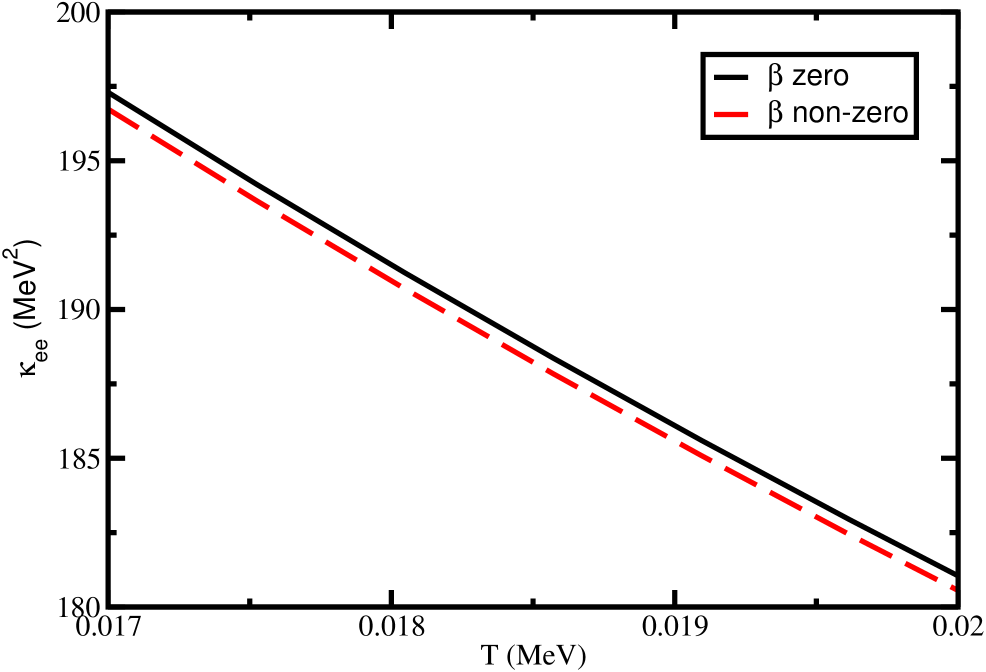
Figure 1: Temperature dependence of the electron thermal conductivity. The left panel shows a comparison between the Fermi liquid and the non-Fermi-liquid NLO result where $\beta\neq 0$. The right panel shows the reduction of $\kappa_{ee}$ with the inclusion of $\beta$.

In this section an estimation of the electron thermal conductivity and the electron thermal relaxation time with the temperature has been presented. In Fig.(1) we have plotted $\kappa_{ee}$ with $T$ using Eq.(40). In the left panel of Fig.(1) we note that the inclusion of both the medium modified propagator and $\beta$ decreases the value of $\kappa_{ee}$. It shows strong deviation from the Fermi liquid result $\kappa_{ee}\propto 1/T$. In the right panel it has been shown that $\beta$ reduces thermal conductivity. This has serious implication on the total electron conductivity $\kappa_{e}$. In [6] the authors have shown that magnetic interaction decreases $\kappa_{ee}$ which in turn increases the electron-electron collision frequency. Thus to the total electron thermal conductivity electron-electron scattering dominates over electron-ion scattering. The phase space correction due to the medium modification of the electron dispersion relation further enhances the electron-electron collision frequency.

With the thermal conductivity and specific heat capacity we further plot the thermal relaxation time with the temperature using Eq.(LABEL:thermal_relax_time). In Fig.(2) we have shown how the thermal relaxation time changes from the FL result with the inclusion of the medium modifications. In the right panel it has been shown that the inclusion of $\beta$ reduces the thermal relaxation time. We have taken the relevant region of temperature and density from the reference [6]. According to [6] in the density region higher than $\rho=10^{6}$ $\text{gcm}^{-1}$ and temperature more than $10^{8}$ K Landau damping becomes important since in this density region non-relativistic degenerate electron plasma becomes relativistic. This region is relevant for our plots.

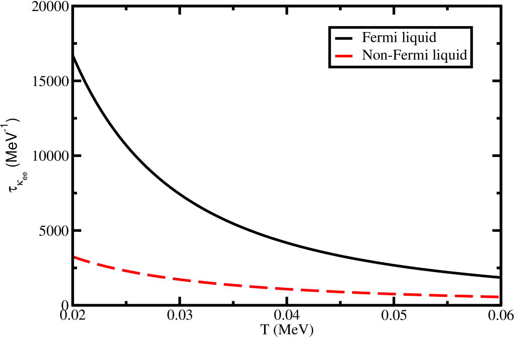
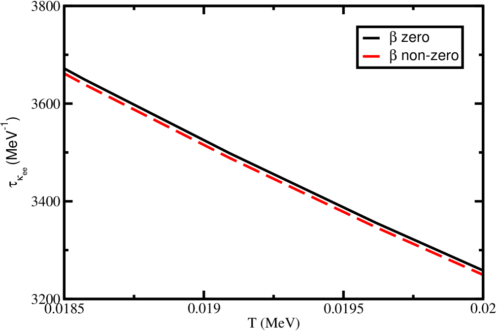
Figure 2: Temperature dependence of the thermal relaxation time. The left panel shows a comparison between the Fermi liquid and the non-Fermi liquid NLO result when $\beta\neq 0$. The right panel shows the reduction of $\tau_{\kappa_{ee}}$ with the inclusion of $\beta$.

IV Summary

In this paper, we calculate the thermal relaxation time in degenerate electron gas in the domain where the relativistic effects become important. It has been shown that with the inclusion of the magnetic interaction, which is relevant in the above mentioned domain, $\tau_{\kappa_{ee}}$ shows departure from the FL behavior. It is known that for the normal FL i.e with only Coulomb interaction $\tau_{\kappa_{ee}}$ behaves as $1/T^{2}$. In the relativistic domain, we on the other hand, find this to be proportional to the inverse temperature i.e $\tau_{\kappa_{ee}}\propto 1/T$. This has been attributed to the absence of screening in the transverse sector. We further expose how the in medium modifications of the electron dispersion characteristic affects the heat conduction from the neutron star crust to the core. Our calculation actually modifies the phase space or the Fermionic density of states as revealed in the text leading to a reduction of conductivity or relaxation time. For the thermal relaxation time, a closed form analytical expression has been derived by making perturbative expansion in $(T/m_{D})$ retaining terms beyond LO. The appearance of the fractional powers in these results are interesting which is reminiscent of what one obtains in the calculation of the fermionic self-energy at high density. Numerically these corrections have also been found to be important in the present context. Particularly these corrections become important in the domain of small frequency i.e when $\omega<<m_{D}$.

Appendix

In this appendix we provide the complete details of the derivation of the energy integral in the phase space factor discussed in the main text. We substitute $-(\epsilon_{p}-\mu)/T=\eta_{p}$, $-(\epsilon_{k}-\mu)/T=\eta_{k}$ and $-\omega/T=z$ to obtain,

$$\int_{0}^{\infty}\,f_{\epsilon_{p}}f_{\epsilon_{k}}(1\pm f_{(\epsilon_{p}+\omega)})(1\pm f_{(\epsilon_{k}-\omega)})d\epsilon_{p}\,d\epsilon_{k}=T^{2}\int_{0}^{\infty}\frac{1}{\left(\text{e}^{-\eta_{p}}+1\right)\left(\text{e}^{(\eta_{p}+z)}+1\right)\left(\text{e}^{-\eta_{k}}+1\right)\left(\text{e}^{(\eta_{k}-z)}+1\right)}d\eta_{p}d\eta_{k}\,.$$ (43)

The lower integration limit can be send to infinity without introducing much error. Now, following [19, 20] the general way to calculate the integral (for a function $f=\eta^{s}$, where s is an integer) as follows,

$$I_{s}=\int_{-\infty}^{\infty}\frac{\eta^{s}}{\texttimes(\text{e}^{-\eta}+1)(\text{e}^{\eta+z})}d\eta=\frac{2}{(1+s)(\text{e}^{z}-1)\texttimes}\sum_{r=0,1,\cdots}^{[\frac{1}{2}s]}(-1)^{s-2r}\dbinom{s+1}{2r}\frac{(s+1)!}{2r!(s+1-2r)!}(2r)!\mathrm{C}_{2r}z^{s+1-2r},$$ (44)

where,

$$2\mathrm{C}_{2r} = \frac{1}{2r!}\int_{-\infty}^{\infty}\eta^{2r}\text{e}^{-\eta}\sum_{0}^{\infty}(1+s)(-1)^{s}\text{e}^{-\eta s}d\eta$$

$$= 2\sum_{0}^{\infty}\frac{(-1)^{s}}{(1+s)^{2r}}.$$ (45)

$[\frac{1}{2}s]$ is the integral part of $\frac{1}{2}s$ and $C_{0}=\frac{1}{2}$. Hence, one can write,

$$T\int_{0}^{\infty}\frac{1}{\left(\text{e}^{-\eta_{p}}+1\right)\left(\text{e}^{(\eta_{p}+z)}+1\right)}\,d\eta_{p}=T\frac{z}{1-\text{e}^{-z}}.$$ (46)

Finally, we obtain the result of the phase space energy integration quoted in Eq.(32) in the main text,

$$\int d\epsilon_{p}\,d\epsilon_{k}\,f_{\epsilon_{p}}f_{\epsilon_{k}}(1\pm f_{(\epsilon_{p}+\omega)})(1\pm f_{(\epsilon_{k}-\omega)})=T^{2}\frac{\frac{\omega^{2}}{4T^{2}}}{\left(\text{sinh}\frac{\omega}{2T}\right)^{2}}.$$ (47)

References

• [1] C. J. Pethick, Rev. Mod. Phys. 64, 1133 (1992).
• [2] J. M. Lattimer, K. A. Van Riper, M. Prakash and M. Prakash Astrophys. J. 425, 802 (1994).
• [3] O. Y. Gnedin, D. G. Yakovlev and A. Y. Potekhin, Mon. Not. R. Astron. Soc. 324, 725 (2001).
• [4] A. Y. Potekhin, D. A. Baiko, P. Haensel and D. G. Yakovlev, Astron. AStrophys. 346, 345 (1999).
• [5] H. Heiselberg and C. J. Pethick, Phys. Rev. D. 48, 2916 (1993).
• [6] P. S. Shternin and D. G. Yakovlev, Phys. Rev. D 74, 043004 (2006).
• [7] P. S. Shternin and D. G. Yakovlev, Phys. Rev. D 75, 103004 (2007).
• [8] A. Gerhold and A. Rebhan, Phys. Rev. D 71, 085010(2005).
• [9] A. Ipp, A. Gerhold and A. Rebhan, Phys. Rev. D 69, R011901(2004).
• [10] A. Gerhold, A. Ipp and A. Rebhan, Phys. Rev. D 70, 105015(2004).
• [11] R. Nandi, S. Banik and D. Bandyopadhyay, Phys. Rev. D 80, 123015(2009).
• [12] S. Sarkar and A. K. Dutt-Mazumder, Phys. Rev. D 84, 096009(2011).
• [13] T. Schafer and K. Schwenzer, Phys. Rev. D 70, 054007 (2004).
• [14] K. Pal and A. K. Dutt-Mazumder, Phys. Rev. D 84, 034004(2011).
• [15] S. P. Adhya, P. K. Roy and A. K. Dutt-Mazumder, arXiv.1204.2684, (2012).
• [16] G. Baym and C. J. Pethick, Landau Fermi-Liquid Theory Concepts and Applications,
(Wiley Interscience, New York, 1991).
• [17] C. Manuel, Phys. Rev. D 53, 5866 (1996).
• [18] M. Le Bellac and C. Manuel, Phys. Rev. D 55, 3215 (1997).
• [19] A. H. Wilson, The Theory of Metals (Cambridge University Press, 1965).
• [20] J. M. Ziman, Electrons and Phonons, The Theory of Transport Phenomena in Solids, (Oxford University Press, Oxford, 1960).