Fast Randomized Model Generation for Shapelet-Based Time Series Classification

Abstract

Time series classification is a field which has drawn much attention over the past decade. A new approach for classification of time series uses classification trees based on shapelets. A shapelet is a subsequence extracted from one of the time series in the dataset. A disadvantage of this approach is the time required for building the shapelet-based classification tree. The search for the best shapelet requires examining all subsequences of all lengths from all time series in the training set.

A key goal of this work was to find an evaluation order of the shapelets space which enables fast convergence to an accurate model. The comparative analysis we conducted clearly indicates that a random evaluation order yields the best results. Our empirical analysis of the distribution of high-quality shapelets within the shapelets space provides insights into why randomized shapelets sampling is superior to alternative evaluation orders.

We present an algorithm for randomized model generation for shapelet-based classification that converges extremely quickly to a model with surprisingly high accuracy after evaluating only an exceedingly small fraction of the shapelets space.

I Introduction

A time series is a sequence of numerical data in which each item is associated with a particular instance in time [1]. These series are the focus of much research in diverse topics such as forecasting, database indexing, clustering and classification [2, 3, 4, 5]. Time series classification is a field which has drawn much attention over the past decade [5, 6, 7, 8, 9, 10].

A new approach for classification of time series, proposed by Ye and Keogh [11], uses shapelets. A shapelet is a subsequence extracted from one of the time series in the dataset. The shapelet is chosen by its ability to split the data into two subsets, such that as many time series as possible belonging to one class will be in one of the subsets. Classifying a time series is done based on whether or not its distance from the shapelet is below a pre-computed threshold value associated with the shapelet. If more than a single shapelet is required, a classification tree is used, with a shapelet placed in each node of the tree. The intuition behind this approach is that the information required to separate the classes is an intrinsic part of the time series behavior expressed best by the measurement values themselves, instead of using summaries of the data. The algorithm of Ye and Keogh considers all the subsequences of the dataset’s time-series in order to identify those shapelets that yield the optimal split. Through the rest of this paper, we will refer to this algorithm as the YK algorithm.

Two key advantages of classification with shapelets are its high accuracy and the interpretability of the classification model learnt. A disadvantage of this approach is the time required for building the classification tree. The search for the best shapelet requires examining all subsequences of all lengths from all time series in the training set. For a small dataset (e.g. 30 time series each with 300 measurements), it may require a few hours to learn the model, as the number of potential shapelets which need to be checked is in the millions (for the example given there are 1,336,530 subsequences which need to be checked). For somewhat larger datasets (e.g. 50 time series each with 1000 measurements leading to 24,925,050 different subsequences) the time required can be measured in days or even weeks.

A number of approaches for reducing the time complexity of shapelet-based model generation have been introduced. McGovern et al. [12] propose an algorithm in which the data is first discretized, and then all subsequences of a minimum predefined length are evaluated, and those deemed best are concatenated to create better motifs for classification. A different approach, proposed by Hartmann et al., uses an evolution strategy to reduce the number of subsequences tested [13]. Both these techniques introduce heuristics for reducing the number of subsequences tested. A method allowing faster analysis of all subsequences was introduced by Mueen et al. [14]. They presented two optimizations, one which can determine whether a subsequence is worth testing or not and another which reduces the time required to test a subsequence which was not dropped in the first step.

I-A Our Contributions

The merits of shapelet based classification motivated us to attempt reducing the time required for generating shaplet-based classification models, thus making use of this approach practical not only for the smallest of datasets. We introduce the ShApLet SAmpling algorithm (henceforth called the SALSA algorithm) for fast computation of shapelet-based classification trees which does not examine all possible shapelets. Instead, the SALSA algorithm samples and evaluates shapelets according to a pre-determined evaluation order only as long as the quality of the new shapelets being examined keeps improving. As part of this process, the distance of each shapelet to all time series is calculated. To speed up the construction of the rest of the classification tree, these distances are saved to disk. Once the quality of new shapelets stops improving, SALSA ceases searching for better shapelets and proceeds to build the rest of the classification tree, using only those shapelets previously examined.

We tested three different shapelet evaluation orders on a number of datasets of varying size with the goal of determining which evaluation order of the shapelets space yields the fastest convergence to an accurate model. The following evaluation orders were implemented and tested: 1) The simple evaluation order iterates through all possible shapelet lengths, from the shortest to the longest, as is done by the YK algorithm. 2) The binary search evaluation order starts with a quick sampling of the shapelets space, by extracting only non-overlapping shapelets of each length. It then iteratively evaluates shapelets of each length, while varying the overlap length of evaluated shapelets in a binary manner (see Section III for more details). 3) The random evaluation order picks a random permutation of the shapelets space and evaluates shapelets according to it, allowing shapelets of all lengths to be examined early on. We henceforth refer to the SALSA algorithm using the random evaluation order as the SALSA-R algorithm.

Our results clearly indicate that the random evaluation order yields the best results of all three approaches. The SALSA-R algorithm converges extremely quickly to a highly accurate model after evaluating only an exceedingly small fraction of the shapelets space. Moreover, it is noteworthy that the accuracy of the shapelets-based model does not monotonically grow as a function of the number of evaluated shapelets. Rather, it grows up to a point (depending on which evaluation order is used) and then starts to decline. Thus, the SALSA-R algorithm can return a model which is even more accurate than that returned by the YK algorithm, which uses all shapelets. We interpret this result as follows: building a model based on too many shapelets makes shapelets-based classification susceptible to overfitting [15].

The time required by the SALSA-R algorithm to converge to a high-accuracy model is orders of magnitude smaller than that of the YK algorithm and, as our experimental evaluation demonstrates, the accuracy of the model it returns is always close to – and often superior to – that of the model returned by the YK algorithm.

Investigation into the reason why random sampling order works so well reveals that there are multiple high-quality shapelets which can be used for building the classification tree, but that they are not evenly distributed through out the shapelets space. From the datasets we analyzed, it seems that all high-quality shapelets are concentrated in a tight cluster of shapelet lengths and all are extracted from the same area in the time series. In light of these results, we believe that the SALSA-R algorithm may be useful in practice for fast generation of accurate shapelets-based classification trees, since an exhaustive search of the shapelets space is exceptionally time consuming.

It is important to note that we are not the first to introduce random shuffling into an algorithm searching for shapelets. The YK algorithm also creates a random permutation of all shapelets of the same length. However, it evaluates shaplets in increasing order of their length. SALSA-R, on the other hand, shuffles all shapelets of all lengths. As our analysis in Section IV establishes, this seemingly small difference is vital for finding high-quality shapelets early on, since high-quality shaplets are concentrated in a very tight range of shaplet-lengths. In addition, our algorithm automatically outputs a classification model upon convergence to a high-accuracy model whereas the YK algorithm examines all shapelets.

The rest of the article is arranged as follows: In section II some definitions are presented as well as a brief description of the YK algorithm. In section III we present our algorithm and three different approaches for defining the order in which shapelets are evaluated. Section IV shows experimental results. Last, section V brings conclusions and presents questions which arise from this work.

II Background

II-A Definitions

Here a number of definitions essential for proper understanding of the article are presented. The following definitions formally describe a time series and measures of similarity between time series.

Definition 1.

A time series $T$ of length $m$ is a series of $m$ successive measurements:

$$T=t_{0},t_{1},...,t_{m-1}$$

Definition 2.

A subsequence $S$ of length $l$ extracted from time series $T$ at position $i$ is a time series of the following form:

$$S=T[i:i+l-1]$$

Definition 3.

The Euclidean distance between two time series $T,V$ of length $m$ is

$$dist_{E}(T,V)=\sqrt{\displaystyle\sum\limits_{i=0}^{m-1}(t_{i}-v_{i})^{2}}$$

Definition 4.

The distance between two time series $T,V$ of different lengths $|T|=m,|V|=m+j,j>0$ is the minimal distance between $T$ and all $j$ subsequences of length $m$ in $V$

The ensuing definitions describe a method for measuring the order induced by a shapelet.

Definition 5.

Let us assume a dataset $D$ with time series from $k$ different classes. We will denote the number of representatives from each class as $C_{i}$. The fraction of time series from each class is $p(C_{i})$ and the entropy of the dataset is:

$$Ent(D)=-\displaystyle\sum\limits_{i=0}^{k-1}p(C_{i})\log{p(C_{i})}$$

Definition 6.

Given a dataset $D$ which is split into two subsets $D_{1},D_{2}$ such that $D_{1}\cap D_{2}=\emptyset$ and $D_{1}\cup D_{2}=D$, the information gain (IG) is the difference between the entropy of $D$ and the weighted average entropy of $D_{1},D_{2}$:

$$IG(D,D_{1},D_{2})=\\ Ent(D)-(p(D_{1})Ent(D_{1})+p(D_{2})Ent(D_{2}))$$

It is worth noting that entropy measures order and that the smaller the entropy the more order there is. This implies that if a certain split of the dataset leads to a more ordered system, the entropy of the subsets will drop and the information gain will increase.

II-B The YK Shapelet Extraction Algorithm

For completeness we briefly describe the YK algorithm as presented in [11]. First, we present the algorithm for two classes; we then extend the description to a multi-class data set. Let $D$ be a dataset with two classes and $N$ time series. The YK algorithm extracts all possible subsequences of every length (from a minimal length, usually 3, to a maximal length which is usually the length of the shortest time series) from every time series. For each subsequence $S$, the distance to each time series is calculated, as defined in def. 4. Then, the time series are ordered by their distance from $S$. Using this induced order, for every two adjacent time series, their average distance to $S$ is calculated. We will refer to this average distance as the splitting distance. Each of the $N$ splitting distances defines two subsets, one containing all time series with a distance to $S$ smaller than or equal to the splitting distance, and the other containing all time series with a distance to $S$ greater than the splitting distance. For every possible split into two subsets, the information gain is calculated. If the current information gain is better than the best so far, the shapelet is kept along with the corresponding splitting distance. Tie breaking is done by keeping the shapelet which gives a larger average distance between the two subsets which is referred to as the margin. After checking all possible subsequences, the best shapelet and the corresponding splitting distance are returned.

This method can be easily extended to a multi-class problem by building a tree, with a shapelet and splitting distance in each node. A new node receives one of the two subsets created by the shapelet found by the node above it, and learns the best shapelet and splitting distance for this subset of time series. The stopping criteria for this recursive algorithm is when all the time series in the subset are from one class.

Two important implementation issues are that all distance calculations are done after local normalization, and that the margin is normalized, by dividing it by the length of the subsequence.

Classification of a time series $t$ is accomplished by walking through the tree. At each node the distance of the shapelet $S$ associated with the node to $t$ is calculated. The node decides to which of its children $t$ should be directed, depending on whether its distance from $S$ is smaller or greater than the splitting distance. When $t$ reaches a leaf, it is assigned the class associated with this leaf.

III The Shaplet Sampling (SALSA) Algorithm

III-A Algorithm Description

The goal of our approach is to provide an accurate classification model as soon as possible. To achieve this, we introduced four major changes to the YK algorithm. First, we changed the order in which shapelets are examined, to allow fast sampling of the entire shapelet domain. Second, our algorithm samples and examines only a small subset of all possible shapelets, ceasing analysis of new shapelets once the quality of shapelets stabilizes. We measure stability by inspecting whether new shapelets improve the IG and margin of the current best shapelet by a significant amount or not, indicating whether a shapelet similar to that with the best IG and margin has been found. Third, while examining shapelets in the root node, the distances of each shapelet to all time series are saved to disk. Last, while building the rest of the classification tree, only those shapelets already examined by the root, with distances to time series already precalculated, are considered as candidates. This eliminates the need to recalculate distances of shapelets to time series in each node.

We describe the SALSA algorithm as a two stage procedure. The first stage, described in procedure 1, searches for the best shapelet for the root node. The second stage, outlined in procedure 2, builds the rest of the tree. The root requires a separate algorithm as the distances of subsequences to time series are as yet unknown, while in the rest of the nodes, these distances have already been calculated. In addition, the root must be able to identify the stabilization of shapelet quality, while the rest of the nodes check all subsequences already considered by the root.

0:   # Input is a dataset and stabilization parameters

0:  

1:  $E\leftarrow enumerator\ of\ shapelets$

2:  Initialize $tree$

3:  $sDst\leftarrow\emptyset$ # Distances of shapelets from time series

4:  $iCnt\leftarrow 0$ # Number of iterations shapelet quality didn’t improve

4:  

5:  repeat

6:     $s\leftarrow E.next()$ # next shapelet to examine

7:     for time series $t$ in $D$ do

8:        $d\leftarrow$ $dist_{E}(s,t)$

9:        $sDst$.push($<s,t,d>$)

10:     Calculate quality of $s$

11:     if shapelet $s$ better than best then

12:        Save (s, splitting distance, IG, margin)

13:     if shapelet quality better than best by more than $\epsilon$ then

14:        $iCnt\leftarrow 0$

15:     else

16:        $iCnt++$

17:  until $iCnt==NI$ or all shapelets have been checked

17:  

18:  $leftD,rightD\leftarrow splitDataset$

19:  $tree.leftTree\leftarrow$ BuildSubTree($leftD,sDst$)

20:  $tree.rightTree\leftarrow$ BuildSubTree($rightD,sDst$)

21:  return  $tree$

Procedure 1 Search for shapelet in Root node

In procedure 1, the input is a dataset of time series $D$ and two parameters defining stabilization: $\epsilon$ and NI. NI (Number of Iterations) defines the number of shapelet-evaluation iterations after which the search for a better shapelet in the root node should terminate in the lack of significant quality improvement. If a shapelet substantially better than the previous best is found, the count is reset to $0$. The amount of change in shapelet quality regarded as substantial is specified by $\epsilon$. Shaplet sampling proceeds if the IG increases by a ratio of at least $\epsilon$ or if the IG remains the same but the margin increases by a ratio of at least $\epsilon$ in the course of the last NI iterations. During initialization (lines 1-4) an enumerator $E$ is initialized, that specifies the sampling order of shapelets; that is, the enumerator defines the order in which the time series subsequences are examined during the algorithm’s execution. The sampling order determined by $E$ is the subject of section III-B. Also in this phase, a data structure to contain the distances of all time series to all shapelets, $sDst$, is initialized, as is a counter $iCnt$, counting the number of iterations since the last substantial change in shapelet quality.

The next segment of code (lines 5-17) describes the analysis of a shapelet by calculating its distance from all time series, determining its ability to split the dataset meaningfully (IG and margin) and evaluating whether it should substitute the current shapelet. In addition, book keeping is done, to promise that distances of subsequences to time series already calculated can be reused by other nodes.

Last, after either stabilization of shapelet quality or examination of all shapelets, the rest of the tree is built (lines 18-20). The dataset is split into two subsets using the splitting distance. All time series with a distance to the chosen shapelet smaller than the learnt splitting distance are assigned to the left subset and the rest are allocated to the right one. Then, for each subset a subtree is built using procedure 2.

Procedure 2 requires a dataset $D$ as well as the data structure containing all shapelets examined and their distances to all time series. As the procedure is recursive (lines 20-21), the base case is checked first, returning a leaf if all time series in $D$ are from one class (lines 2-3).

Next, all shapelets examined by the root, which were extracted from $D$ (as $D$ is only a subset of the original dataset, some of the shapelets may have been extracted from time series not in this particular subset) are examined in the same fashion as in procedure 1.

Two special edge cases are if none of the shapelets in $sDst$ were extracted from time series in subset $D$ (lines 13-15) or if the best shapelet found by this node couldn’t split $D$ into two non-empty subsets (lines 16-18). In both these cases, a leaf is created as an attempt to build a sub-tree would lead to infinite recursion. The class assigned is decided by a majority vote (i.e. the class with the most representatives) breaking ties by choosing the class with the smaller value.

0:   # Input is a dataset and all shapelets already examined with their distances all time series

0:  

1:  Initialize $tree$

2:  if all time series in $D$ are from one class then

3:     return  Leaf representing class

3:  

4:  repeat

5:     $s\leftarrow sDst.next()$ # next shapelet to examine

6:     if $s$ was extracted from $D$ then

7:        Calculate quality of $s$

8:        if shapelet $s$ better than best then

9:           Save (s, splitting distance, IG, margin)

10:     else

11:        continue

12:  until all shapelets have been checked

12:  

13:  if $sDst$ contains no shapelets extracted from $D$ then

14:     Decide class by majority vote

15:     return  Leaf representing class

16:  if $D$ couldn’t be split by best shapelet then

17:     Decide class by majority vote

18:     return  Leaf representing class

18:  

19:  $lDataset,rDataset\leftarrow splitDataset$

20:  $tree.leftTree\leftarrow$ BuildSubTree($lDataset,sDst$)

21:  $tree.rightTree\leftarrow$ BuildSubTree($rDataset,sDst$)

22:  return  $tree$

Procedure 2 Building a sub-tree

III-B Shapelets Sampling Order

Here we elaborate on line 1 of procedure 1, which introduced an enumerator of the shapelets, determining the order in which shapelets are considered by the algorithm. Following are three different procedures, each specifying a different sampling order. The pseudo-code of these procedures specifies the order in which the shapelets domain is enumerated. In other words, calls of the next method implemented by an enumerator output shapelets in the order prescribed by the corresponding procedure.

The first enumeration order, sketched in procedure 3, simply iterates through all possible shapelet lengths from shortest to longest, extracting all shapelets from each time series. The second, described in procedure 4, samples the entire shapelets domain quickly, by extracting only non-overlapping shapelets of each length in every iteration of the outer loop (line 3) instead of extracting all shapelets of each length at once. An important parameter is startIndex, which defines the index in the time series from which we start extracting the non-overlapping subsequences (each start index between 0 and the length of the subsequence will define a different set of non-overlapping subsequences). We defined the function nextStartIndex (line 7) to enhance the procedure’s ability to promise fast coverage by choosing $startIndex$ intelligently. Iteration over the start indices is done in a manner resembling a binary search, hence the procedure’s name, always defining the next start index as the middle between two previously examined start indices. For example, if extracting subsequences $8$ measurements long, the order of the start indices would be as follows: $[0,4,2,6,1,3,5,7]$. The first start index is $0$. The next start index is calculated as halfway between examined indices (0,8) etc. This combination of extraction of non-overlapping subsequences and the special way in which the next start index is determined are meant to ensure that we quickly sample the entire subsequence domain and that a subsequence very similar to the best shapelet will be encountered early on. The last method, depicted in procedure 5, enumerates shapelets according to the order defined by a random permutation of the entire shapelets space.

0:   # Input is a dataset

0:  

1:  $minLen\leftarrow 3$

2:  $maxLen\leftarrow$ length of shortest time series

2:  

3:  for subsequence length $l$ from $minLen$ to $maxLen$ do

4:     for time series $t$ in $D$ do

5:        $lastIndex\leftarrow$ (t.length - l +1)

6:        for index $i$ from $0$ to $lastIndex$ do

7:           $subseq\leftarrow t[i:i+l-1]$

8:           output($subseq$)

9:  return  $E$

Procedure 3 Simple enumeration of shapelets domain

0:   # Input is a dataset

0:  

1:  $minLen\leftarrow 3$

2:  $maxLen\leftarrow$ length of shortest time series

2:  

3:  repeat

4:     for subsequence length $l$ from $minLen$ to $maxLen$ do

5:        if all subsequences of this length have been extracted then

6:           continue

7:        $startIndex\leftarrow$ nextStartIndex()

8:        for time series $t$ in $D$ do

9:           $lastIndex\leftarrow$ (t.length - l +1)

10:           for index $i=0;\ i\leq lastIndex;\ i=i+l$ do

11:              $subseq\leftarrow t[i:i+l-1]$

12:              output($subseq$)

13:  until all subsequences have been extracted

14:  return  $E$

Procedure 4 Fast-coverage enumeration of shapelets domain

0:   # Input is a dataset

0:  

1:  $P\leftarrow$ random permutation of shapelets domain

2:  output shaplets according to the order defined by $P$

Procedure 5 Random enumeration of shapelets domain

In [11, 14], optimizations for the original algorithm were introduced. Some accelerate the distance calculations and some allow pruning of shapelets before their distance to all time series have been computed. The SALSA algorithm can encompass any of the optimizations accelerating the distance calculations, but cannot include those which prune shaplets as pruning methods can reject a shapelet before its distance to all time series has been calculated. In the SALSA algorithm, the distances of the shapelets to the time series are required not only by the root but also by the other nodes in the tree: a shapelet that is useless in the root may be the best shapelet for a subset of the dataset assigned to one of the inner nodes.

IV Experimental Results

The purpose of our experiments was threefold. First, we compared the performance of the three different enumeration orders in which shapelets are examined, described in section III-B. Our objective was to find which enumeration order allows returning the most accurate model fastest. Second, after having found that the randomized evaluation order is significantly better than the alternative evaluation orders, we analyzed the distribution of high-quality shapelets within the datasets at hand in order to gain insights into the reasons underlying that. Third, we analyzed the performance and accuracy of the SALSA algorithm using the random evaluation order (SALSA-R) and compared it with those of the YK algorithm.

IV-A Comparison of Shaplets Evaluation Orders

IV-A1 Experimental Setup

We tested the three different shaplet evaluation orders on all one-dimensional datasets on which the YK algorithm was assessed: arrowhead, coffee, mallat, shield and wheat. Two additional datasets we used were ecgPatterns and controlCharts. We split ecgPatterns into two, using the first half of the dataset for training and the second half for testing. All datasets are available online [16],[17],[18]. Table I summarizes important features of the datasets we used: the size of a dataset refers to the number of time series and the time series length measures the length of the shortest time series in the training set. As can be seen, the training sets vary in size and in number of classes.

The arrowhead dataset describes different types of arrowheads classified by the geographic location in which they were found. The shield dataset contains shapes of shields used in different places and during different eras, as depicted in historical documents. Wheat and coffee both contain spectrographs of different strains, with a goal of distinguishing between them. ControlCharts and mallat are both synthetically generated datasets, used for testing different classification methods.

TABLE I: Information on Datasets

Dataset	train set	test set	#classes	time series
	size	size		length
arrowhead	36	175	3	340
coffee	28	28	2	286
controlCharts	200	400	6	60
ecgPatterns	100	100	4	40
mallat	320	2080	8	256
shield	30	129	3	994
wheat	49	726	7	1050

To assess how the accuracy of the model evolves over time using each of the three methods for ordering the shapelets, we implemented the YK algorithm and tested its performance as it evaluates shapelets in the order prescribed by these methods. We halt the algorithm at a pre-determined number of test points. At each such test point, the process of examining new shapelets in the root is halted and a classification tree using only the shapelets already examined is built. Test points are set so that the number of shaplets evaluated between every two test points is equal. The accuracy of the models built at these test points is determined based on the dataset’s test set.

For mallat, we use 50 test points and for the rest of the datasets we use about 500 test points. The reason for evaluating performance on mallat using only 50 test points is that due to its size, significantly more time is required to build the classification tree as compared with the other data sets. Results for the random evaluation order can vary, therefore we executed the experiment 10 times and averaged the accuracy at each test point.

IV-A2 Performance Measures

Evaluation of the classification trees was done by computing the percentage of time series which were correctly classified from all time series in the test set.

Comparing performance of different algorithms requires special consideration. In many cases, simply comparing algorithms’ running times does not seem to be the best measure as it highly depends on the runtime environment used, and on the quality of the code used to implement the algorithm. Consequently, many works use a measure that abstracts away these factors [19, 20, 21]. We take a similar approach. Our experimental evaluation uses the number of shapelets examined by an algorithm as a measure of the work done by it. We thus assess the accuracy obtained by an algorithm, as a function of the number of shapelets it evaluates.

IV-A3 Examination of Ordering Methods

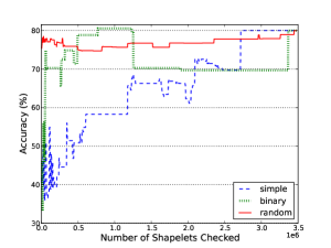
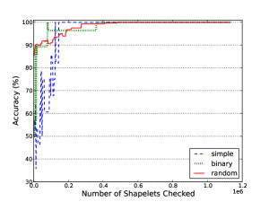
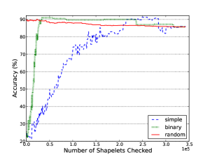
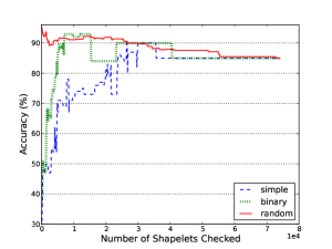
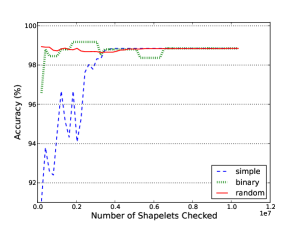
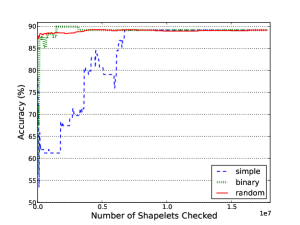
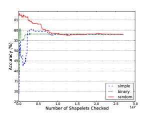
Fig. 1 shows the results of our experiments. For each dataset, there is a separate diagram showing the accuracy of each of the orderings as a function of the number of shapelets examined. We ran the random method 10 times, the red line showing the average accuracy at each point. The graphs clearly show that, whereas the initial accuracy of simple and binary are rather low, the initial accuracy of random is extremely close to the accuracy after searching the entire shapelets space, in many cases even surpassing it.

The graphs also show that accuracy does not necessarily increase with the number of shapelets examined, although the trend is usually positive. Declines in accuracy after inspecting additional shapelets can be seen in all datasets. Moreover, for random the trend is in some cases negative, with the accuracy of the first models outperforming that of the final model (Fig. 1 1(c),1(d),1(g)). These declines in accuracy can be interpreted as a manifestation of overfitting [15] which states that searching for the model which best fits the training set may memorize peculiarities of the training set, instead of finding a more general rule.

Averaging many samples smoothes the curvature of a graph. As we averaged the results from 10 executions of the random method, the smooth behavior of the graph showing the accuracy of the random method may be a side effect of averaging and not represent the true behavior of the algorithm. We performed a simple test presented in Table II, to check whether there are sharp fluctuations in accuracy obtained by our random method, not seen in the graphs due to smoothing. For each dataset, from all 10 experiments, we chose the minimal and maximal accuracy obtained anywhere during the experiment. For the majority of datasets the minimal accuracy is within 10% of the final accuracy (that obtained after all shapelets have been examined) and the maximal accuracy usually surpasses it. It is therefore safe to say that our averaging does not hide sharp fluctuations in accuracy.

Clearly from Fig. 1, random shapelet sampling converges extremely fast to an accurate model and invariably provides models that are significantly superior to those obtained by the other evaluation orders for the first test points.

(a) arrowhead

(b) coffee

(c) controlCharts

(d) ecgPatterns

(e) mallat

(f) shield

(g) wheat

Figure 1: Comparison of three enumeration methods for searching for the best shapelet. Blue is simple, green is binary and red is random.

TABLE II: Variance in Random

Dataset	Min	Max	Final
arrowhead	64.0%	82.9%	80.0%
coffee	78.6%	100.0%	100.0%
controlCharts	81.7%	93.5%	85.7%
ecgPatterns	83.0%	98.0%	85.0%
mallat	98.0%	99.6%	98.8%
shield	84.5%	90.7%	89.1%
wheat	52.3%	72.6%	58.0%

IV-B Analysis of High-Quality Shapelets Distribution

To understand why random sampling converges so quickly to a high-accuracy model, we measured the quality of all shapelets (in terms of information gain (IG) and margin) in each of the datasets described in table I. We extracted all shapelets with IG within $10\%$ of and margin within $40\%$ of those of the best shapelet for the root. We chose these bounds on shapelet quality, as we noticed that in the previous experiment all models with high accuracy came from within this range.

The focus of our analysis was to determine whether high-quality shapelets are evenly distributed throughout the shapelet space, or whether they are concentrated in certain areas. In this context, even distribution means that shapelets of all lengths, from any position in the time series, have equal probability of achieving good quality measures.

(a) arrowhead

(b) coffee

(c) controlCharts

(d) ecgPatterns

(e) mallat

(f) shield

(g) wheat

Figure 2: Histograms of high-quality shapelet concentrations. Axes are the lengths of the shapelets and the positions in the time series from which they were extracted

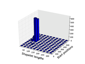
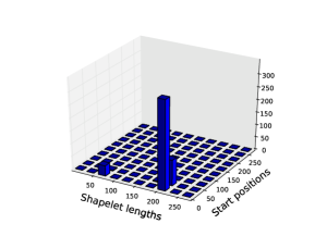
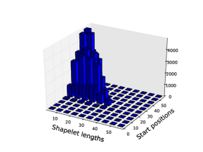
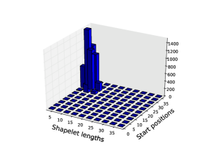
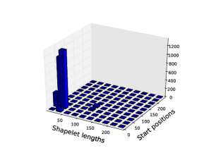
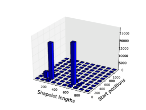
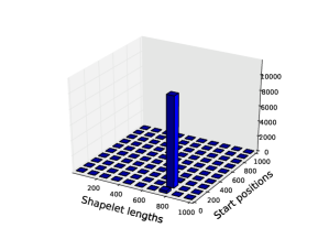
Fig. 2 shows the numbers of high-quality shapelets of different lengths and different offsets within the time series. It is evident that high-quality shapelets are not evenly distributed through out the shapelet space; rather they are concentrated in clusters. This fits with the main concept of shapelet classification, that there are specific areas inside time series which contain the classes “fingerprint”, allowing differentiation between different classes.

As high-quality shapelets all appear in a particular area of the shapelet space, scanning the entire space starting with the shortest length and continuing incrementally to shapelets of the longest length will, in most cases, require examining a considerable number of shapelets before reaching high-quality shapelets. This is the reason that both the simple and the binary orderings do not attain high accuracy as early on as random ordering. This is also the reason that the enumeration used by the YK algorithm does not generally achieve high accuracy early on. Although the YK algorithm creates a random permutation of all shapelets within each length, it nevertheless enforces examination of shapelets from shortest to longest length.

As it is not known a priori where high-quality shapelets are clustered within the shapelets space, random sampling across different shapelet lengths and offsets is required.

IV-C Performance of the SALSA-R Algorithm

After establishing that random is the best sampling order and gaining insights into why this is so, we proceed to evaluate the SALSA-R algorithm. As we described in Section III-A, the SALSA-R algorithm uses the random evaluation order and outputs a classification model upon convergence to a high-accuracy model.

IV-C1 Experimental setup

We evaluated SALSA-R on all datasets presented in table I. The value for $\epsilon$ was 0.01, i.e. our algorithm considers a shapelet as significantly better if its IG or margin are better by a factor of at least $1\%$. For the number of iterations NI, after which SALSA-R terminates if no significant improvement in shapelet quality was observed, we tested two values: $10,000$ and $100,000$. For each combination of $\epsilon$ and NI and for each dataset, we executed our procedure $20$ times, due to the element of randomness.

IV-C2 Experimental Results

For each dataset, we calculated the average accuracy, number of shapelets examined and the running time. The results are presented in table  III. For each measure we present the values obtained using $NI=10,000$, $NI=10,0000$ and those achieved by prior art. By prior art we refer to both the YK algorithm and to a more optimized implementation described in [14]. When we could, we compared with the faster procedure (available at [22]) which can discard a shapelet by comparing it to previously examined shapelets, but due to large RAM consumption, for datasets mallat, shield and wheat, we compared with the YK algorithm (for mallat, the YK algorithm did not terminate after more than two weeks so we compared with the accuracy published in [11]). Next to each average accuracy, we recorded the standard deviation in brackets.

TABLE III: Performance of self terminating algorithm with $\epsilon=0.01$ and $NI=10,000,\ \ 100,000$

Dataset	Accuracy($\%$) (std)			number of shapelets			time (sec)
	NI=10,000	NI=100,000	Prior Art	NI=10,000	NI=100,000	Prior Art	NI=10,000	NI=100,000	Prior Art
arrowhead	78.1 (4.5)	78.4 (2.8)	80.0	1.8e4	1.6e5	1.6e6	28.7	254.0	2444.2
coffee	91.4 (5.3)	95.0 (5.6)	100.0	1.6e4	1.7e5	1.1e6	10.4	103.1	492.7
controlCharts	89.2 (2.5)	87.1 (1.4)	85.7	1.2e4	1.5e5	3.4e5	9.5	112.6	1613.2
ecgPatterns	90.3 (3.1)	85.0 (0.0)	85.0	1.1e4	7.4e4	7.4e4	2.2	15.0	90.0
mallat	99.0 (0.4)	98.7 (0.7)	98.8	1.8e4	1.8e5	1.0e7	114.4	954.0	$>$1.2e6
shield	87.3 (1.3)	88.1 (1.3)	89.1	1.6e4	1.6e5	1.7e7	135.6	994.3	4.2e5
wheat	67.7 (2.2)	69.2 (2.0)	58.0	1.6e4	1.7e5	2.7e7	214.1	1773.6	5.1e5

For all datasets except one, the accuracy we achieve is very close to that of prior art (within $2\%$), and for three of the datasets our algorithm improves the accuracy obtained. Also, the standard deviation is relatively small, indicating that the expected accuracy of any single model should be close to the average value. The numbers of shapelets checked show that SALSA-R examines only a small fraction of the shapelets space (except for ecgPatterns and controlCharts which are small datasets), in some cases only $1/1000$ of all shapelets, while still attaining high accuracy. Naturally, the number of shapelets examined is reflected in the time required to build a model, as recorded in the last three columns of table  III. For small datasets, our algorithm terminates (on average) after a few seconds, compared with previous algorithms which require a number of minutes. For larger datasets, a good model is computed within a few minutes instead of a number of days. This comparison establishes that for most datasets, the SALSA-R algorithm outputs an accurate model using only a very small fraction of the shapelets required by the pruning method and requiring only a small fraction of the time. Moreover, the performance boost gained by SALSA-R grows quickly with the size of the dataset.

V Conclusions

The focus of our work was acceleration of the time taken to build a model for shapelet-based classification. To this end, we compared different orders for shaplet evaluation, concluding that from all those examined, the random order is best. Our work establishes that the reason for this is that shapelets are not evenly distributed through out the entire shapelets space. Rather, they are concentrated in a tight cluster of shapelet lengths and locations in time series. Consequently, fast identification of high-quality shapelets requires quick sampling of the entire shapelets space.

We implemented SALSA-R, an algorithm that samples shaplets randomly and uniformly from the shapelets space and outputs a classification tree model upon observing that the quality of sampled shapelets stabilizes. Our evaluation shows that SALSA-R outputs an accurate model after evaluating only a small fraction of the number of shapelets required by prior art shapelet-based learning algorithms, requiring only a small fraction of their time. A novel observation stemming from our work is that considering too many shapelets may lead to a decrease in model accuracy, most probably because of overfitting.

In the future we plan to attempt to further increase the accuracy and reduce the time-complexity of our algorithm. One direction is to try alternative sampling strategies. For instance, accuracy may be improved by initially performing random and uniform sampling of the shaplets space and then reverting to a more thorough search of specific areas in which a significant number of high-quality shaplets were found. The current measure for shaplet quality is its information gain and margin. Another avenue for future work is to investigate alternative shapelet quality criteria.

References

- [1] R. Harris and R. Sollis, Applied time series modelling and forecasting. J. Wiley, 2003.
- [2] R. Agrawal, C. Faloutsos, and A. Swami, “Efficient similarity search in sequence databases,” Foundations of Data Organization and Algorithms, pp. 69–84, 1993.
- [3] C. Faloutsos, M. Ranganathan, and Y. Manolopoulos, “Fast subsequence matching in time-series databases,” ACM SIGMOD Record, vol. 23, no. 2, pp. 419–429, 1994.
- [4] W. Liao et al., “Clustering of time series data–a survey,” Pattern Recognition, vol. 38, no. 11, pp. 1857–1874, 2005.
- [5] P. Geurts, “Pattern extraction for time series classification,” Principles of Data Mining and Knowledge Discovery, pp. 115–127, 2001.
- [6] M. Kadous and C. Sammut, “Classification of multivariate time series and structured data using constructive induction,” Machine learning, vol. 58, no. 2, pp. 179–216, 2005.
- [7] E. Keogh and M. Pazzani, “An enhanced representation of time series which allows fast and accurate classification, clustering and relevance feedback,” in Proceedings of the 4th International Conference of Knowledge Discovery and Data Mining, 1998, pp. 239–241.
- [8] R. Povinelli, M. Johnson, A. Lindgren, and J. Ye, “Time series classification using Gaussian mixture models of reconstructed phase spaces,” Knowledge and Data Engineering, IEEE Transactions on, vol. 16, no. 6, pp. 779–783, 2004.
- [9] C. Ratanamahatana and E. Keogh, “Making time-series classification more accurate using learned constraints,” in Proceedings of SIAM International Conference on Data Mining. Lake Buena Vista, Florida, 2004, pp. 11–22.
- [10] X. Xi, E. Keogh, C. Shelton, L. Wei, and C. Ratanamahatana, “Fast time series classification using numerosity reduction,” in Proceedings of the 23rd international conference on Machine learning. ACM, 2006, pp. 1033–1040.
- [11] L. Ye and E. Keogh, “Time series shapelets: a novel technique that allows accurate, interpretable and fast classification,” Data Mining and Knowledge Discovery, pp. 1–34, 2011.
- [12] A. McGovern, D. Rosendahl, R. Brown, and K. Droegemeier, “Identifying predictive multi-dimensional time series motifs: an application to severe weather prediction,” Data Mining and Knowledge Discovery, vol. 22, pp. 232–258, 2011.
- [13] B. Hartmann, I. Schwab, and N. Link, “Prototype optimization for temporarily and spatially distorted time series,” in the AAAI Spring Symposia, 2010.
- [14] A. Mueen, E. Keogh, and N. Young, “Logical-shapelets: an expressive primitive for time series classification,” in Proceedings of the 17th ACM SIGKDD international conference on Knowledge discovery and data mining. ACM, 2011, pp. 1154–1162.
- [15] T. Dietterich, “Overfitting and undercomputing in machine learning,” ACM Comput. Surv., vol. 27, no. 3, pp. 326–327, Sep. 1995. [Online]. Available: http://doi.acm.org/10.1145/212094.212114
- [16] “Ecg dataset,” http://www.cs.ucr.edu/~wli/ICDM05/.
- [17] “shapelet datasets,” http://alumni.cs.ucr.edu/~lexiangy/shapelet.html.
- [18] E. Keogh, Q. Zhu, B. Hu, H. Y., X. Xi, L. Wei, and C. A. Ratanamahatana, “The ucr time series classification/clustering homepage,” www.cs.ucr.edu/~eamonn/time_series_data/, 2011.
- [19] L. Chen and R. Ng, “On the marriage of lp-norms and edit distance,” in Proceedings of the Thirtieth international conference on Very large data bases-Volume 30. VLDB Endowment, 2004, pp. 792–803.
- [20] H. Ding, G. Trajcevski, P. Scheuermann, X. Wang, and E. Keogh, “Querying and mining of time series data: experimental comparison of representations and distance measures,” Proceedings of the VLDB Endowment, vol. 1, no. 2, pp. 1542–1552, 2008.
- [21] L. Wei, E. Keogh, H. Van Herle, and A. Mafra-Neto, “Atomic wedgie: efficient query filtering for streaming times series,” 2005.
- [22] “logical shapelet webpage,” http://www.cs.ucr.edu/~mueen/LogicalShapelet/.