Estimating Player Contribution in Hockey with Regularized Logistic Regression

Abstract

We present a regularized logistic regression model for evaluating player contributions in hockey. The traditional metric for this purpose is the plus-minus statistic, which allocates a single unit of credit (for or against) to each player on the ice for a goal. However, plus-minus scores measure only the marginal effect of players, do not account for sample size, and provide a very noisy estimate of performance. We investigate a related regression problem: what does each player on the ice contribute, beyond aggregate team performance and other factors, to the odds that a given goal was scored by their team? Due to the large-$p$ (number of players) and imbalanced design setting of hockey analysis, a major part of our contribution is a careful treatment of prior shrinkage in model estimation. We showcase two recently developed techniques – for posterior maximization or simulation – that make such analysis feasible. Each approach is accompanied with publicly available software and we include the simple commands used in our analysis. Our results show that most players do not stand out as measurably strong (positive or negative) contributors. This allows the stars to really shine, reveals diamonds in the rough overlooked by earlier analyses, and argues that some of the highest paid players in the league are not making contributions worth their expense.

Key words: Logistic Regression, Regularization, Lasso, Bayesian Shrinkage, Sports Analytics

1 Introduction

Player performance in hockey is difficult to quantify due to the continuity of play, frequent line changes, and the infrequency of goals. Historically, the primary measure of individual skater performance has been the plus-minus value: the number of goals scored by a player’s team minus the number of goals scored by the opposing team while that player is on the ice.

More complex measures of player performance have been proposed to take into account game data beyond goal scoring, such as hits or face-offs. Examples include the adjusted minus/plus probability approach of Schuckers et al., (2010) and indices such as Corsi and DeltaSOT, as reviewed by Vollman, (2010). Unfortunately, analysts do not generally agree on the relative importance of the added information. While it is possible to statistically infer additional variable effects in a probability model for team performance Thomas et al., (2012) our experience is that, in the low-scoring world of hockey, such high-dimensional estimation relies heavily upon model assumptions that are difficult to validate. As a result, complex scores provide an interesting new source of commentary but have yet to be adopted as consensus performance metrics or as a basis for decision making.

Due to its simplicity, the plus-minus remains the most popular measure of player performance. It has been logged for the past fifty years and is easy to calculate from the current resolution of available game data, which consists of the identities of each player on the ice at any time point of the game as well as the times when goals were scored. However, a key weakness is that the plus-minus for each player does not just depend on their individual ability but also on other factors, most obviously the abilities of teammates and opponents.

In statistical terms, plus-minus is a marginal effect: it is an aggregate measure that averages over the contributions of opponents and teammates. Since the quality of the pool of teammates and opponents that each player is matched with on-ice can vary dramatically, the marginal plus-minus for individual players are inherently polluted. Another disadvantage is that plus-minus does not control for sample size, such that players with limited ice-time will have high variance scores that soar or sink depending on a few chance plays.

A better measure of performance would be the partial effect of each player, having controlled for the contributions of teammates, opponents and possibly other variables. To this end, we propose a logistic regression model to estimate the credit or blame that should be apportioned to each player when a goal is scored. In keeping with the spirit of plus-minus (and using the same publicly available data), we focus on the list of players on the ice for each goal as our basic unit of analysis. Briefly, denote by $q_{i}$ the probability that a given goal ‘$i$’ was scored by the home team (home and away are just organizational devices; results are unchanged upon modeling $\mathrm{p}(away)$ instead). Then

$$\log\left(\frac{q_{i}}{1-q_{i}}\right)=\alpha_{i}+\beta_{h_{i1}}+\ldots+\beta_{h_{i6}}-\beta_{a_{i1}}\ldots-\beta_{a_{i6}},$$ (1)

where $\boldsymbol{\beta}=[\beta_{1}\cdots\beta_{n_{p}}]^{\prime}$ is the vector of partial plus-minus effects for each of $n_{p}$ players in our sample, with $\{h_{i1}\ldots h_{i6}\}$ and $\{a_{i1}\ldots a_{i6}\}$ being the indices on $\boldsymbol{\beta}$ corresponding to home-team ($h$) and away-team ($a$) players on the ice for goal $i$. The intercept term $\alpha_{i}$ can depend upon additional covariates, e.g. the model we present in Section 2.2 incorporates team indicators into $\alpha_{i}$.

In almost all regressions, one is susceptible to the twin problems of over-fit, where parameters are optimized to statistical noise rather than fit to the relationship of interest, and multicollinearity, where groups of covariates are correlated with each other making it difficult to identify individual effects. These issues are especially prominent in analysis of hockey, with a high dimensional covariate set (around 1500 players in our sample) and a very imbalanced experiment design – due to use of player lines, wherein groups of 2-3 players are consistently on ice together at the same time, the data contain many clusters of individuals who are seldom observed apart.

A crucial contribution of our paper is a careful treatment of the partial player effects $\boldsymbol{\beta}$ that helps alleviate both problems. As outlined in Section 2.2, a prior distribution with its mode at the origin is placed on each $\beta_{j}$; this adds a penalty – e.g., $\lambda_{j}\beta_{j}^{2}$ or $\lambda_{j}|\beta_{j}|$ – on the likelihood function and shrinks estimates of this coefficient towards zero. We use the term regularization to refer to the shrinkage of regression coefficients towards zero that is induced by our prior distribution.

Building on new developments in regularized estimation for regression with binary response (such as our home-vs-away outcome), we leverage machinery that has only very recently become available for data sets of the size encountered in our analysis. In particular, we detail penalized likelihood maximization for fast robust estimates of player contribution, as well as Bayesian simulation for exploring joint uncertainty in multiple player effects, allowing for comparisons between groups of players which would not have been possible with earlier methodology. In both cases, inference proceeds through simple commands to newly developed packages for the open source R analysis software (R Development Core Team,, 2010). The resulting player effects are easy to interpret, and our hope is that readers will experiment with our models to feed a discussion on alternative plus-minus metrics.

The remainder of the paper is outlined as follows. Section 1.1 provides an overview of previous attempts at a partial player affect. These avoid full-scale logistic regression which, until very recently, would not have been computationally feasible. Section 2 details our data and general regression model. Section 3 presents point estimates of player effects, comparing results both with and without controlling for teams and under a range of levels of prior regularization. These regularized point estimates can be used for variable selection, since only a subset of effects will be non-zero. Section 4 then describes a full Bayesian analysis of the joint uncertainty about players, and illustrates how such information can be used by coaches and general managers to make important personnel decisions. The paper concludes in Section 5 with a discussion, and an appendix which contains details of our estimation algorithms and the entertainment of a full interaction model.

1.1 Background on Adjusted Plus-Minus

The strategy of conditional estimation for player ability is not new to sports analysis. For example, Awad, (2009) advocates a simple adjustment to hockey plus-minus that controls for team strength by subtracting team-average plus-minus. Basketball analysts have been active with conditional performance models, including the linear regressions employed by Rosenbaum, (2004) and Ilardi and Barzilai, (2004). Due to frequent scoring and variability in the combination of players on the floor, estimation of partial effects is generally easier in basketball than in the low scoring and imbalanced design setting of hockey.

For hockey, Macdonald, (2010) proposes analysis of the relationship between players and goals through regression models similar to those used in basketball. He tracks the length of time on ice and goals scored in each of around 8$\times 10$⁵ “shifts” – unique combinations of players – to build a goals-per-hour response that is regressed onto player effect variables analogous to our $\boldsymbol{\beta}$ in (1). While Macdonald’s work is related to ours, as both are regressing scoring onto player presence, we outline several distinctions between the approaches which are helpful in understanding the motivation behind our modeling.

The use of shift-time (regardless of whether a goal was scored) introduces extra information but also leads to questions on data quality and model specification. For example, we find a median actual shift length of eight seconds, such that the recorded total time-on-ice for unique player combinations is built from pieces that may be too small for play to develop or be assessed. The average goals-per-shift is around 0.02 such that less than 2% of the sampled response is nonzero. This calls into doubt the assumption of approximate normality upon which Macdonald’s standard error estimates are based. Moreover, although there are more observations in the sample than there are covariates, a vast majority of scoreless shifts implies that least-squares estimation is dominated by a few scoring shifts. Even with a more balanced sample, estimation on this dimension is likely overfit without regularization. Indeed, Macdonald reports only top skaters among those with at least 700 minutes on ice; we suspect that players with very little ice time dominate the full list of effects.

2 Data and Model

This section details our data, the full regression model, and prior specification.

2.1 Data

The data, downloaded from www.nhl.com, comprise of information about the teams playing (with home/away indicators), and the players on ice (including goalies) for every even strength goal during the four regular seasons of 2007–2008 through 2010–2011. There were $n_{p}=1467$ players involved in $n_{g}=18154$ goals. In keeping with the canonical definition of plus-minus, we do not consider power-play/shorthanded or overtime goals; however, our framework is easily extended to handle such data.

This article focuses on the 4-season data aggregate and treats player ability as constant over this range. The larger data window allows for better effect measurement, especially due to the increased variation in on-ice configuration and player movement between teams. However, different aggregations will be desirable for different situations and one can apply our methods to any subset. Given a data window that is too short for measurement of individual ability, our sparse estimation methods will simply set all player effects to zero.

The data are arranged into a response vector $Y$ and a design matrix $X$ comprising of two parts, $X_{T}$ and $X_{P}$, for indicator variables corresponding to team and player identities respectively. For each goal $i$ the response vector contains $y_{i}=1$ for goals scored by the home team and $y_{i}=-1$ for away team goals. The corresponding $i^{\mathrm{th}}$ row of $X$ indicates the teams playing and the players on the ice when that goal was scored, with $x_{Tij}$ equal to 1 for the home team and $x_{Pij}$ equal to 1 for each home player on the ice, and $x_{Tij}$ equal to $-1$ for the away team and $x_{Pij}$ equal to $-1$ for each away player on the ice. All other $x_{Tij}$ and $x_{Pij}$ indicators are equal to zero. Figure 1 illustrates this data structure with two example rows.

Figure 1: A diagram of the design matrix and two example rows. Two goals are shown under the same configuration of teams and players, except that the home team has scored in the first case and the visiting team in the second (so that the two rows have opposite parity). Exactly two teams have nonzero entries and exactly twelve players (six home, six away) are nonzero in each row.

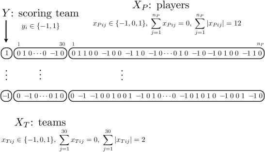
Note that the design matrix is extremely sparse: overall dimensions are $n_{g}\times(n_{p}+30)=18154\times 1497$, but every row has 1485 zeros for more than 99% sparsity. As already noted, the design is also highly imbalanced: only about 27K of the greater than one million possible player pairs are actually observed on the ice for a goal.

2.2 Logistic Likelihood Model

From the data definition of 2.1, we can reformulate our logistic regression equation of (1) as

$$\log\left(\frac{q_{i}}{1-q_{i}}\right)=\mathbf{x}_{Ti}^{\prime}\boldsymbol{\alpha}+\mathbf{x}_{Pi}^{\prime}\boldsymbol{\beta}$$ (2)

where $q_{i}=\mathrm{p}(y_{i}=1)$, $\mathbf{x}_{Pi}=[x_{Pi1}\cdots x_{Pin_{p}}]^{\prime}$ is the vector corresponding to the $i^{th}$ row of $X_{P}$, $\mathbf{x}_{Ti}$ is similarly the $i^{th}$ row of $X_{T}$, $\boldsymbol{\alpha}$ is the length-30 vector of team effects and $\boldsymbol{\beta}$ is the length-$n_{p}$ vector of player effects.

The likelihood model in (2) is easily extended to incorporate additional conditioning information or more flexible player-effect specifications. For example, $\mathbf{x}_{Ti}$ and $\boldsymbol{\alpha}$ could be lengthened to account for special teams effects (e.g., including variables to indicate penalties or other non-five-on-five situations) or potential sources of bias (e.g., referee indicators). Moreover, $\mathbf{x}_{Pi}$ and $\boldsymbol{\beta}$ could be doubled in length to include distinct offensive and defensive player effects, as in Ilardi and Barzilai, (2004). We focus on the current formulation to stay true to the spirit of the standard plus-minus metric, although we do investigate a model with pairwise interactions between players in Appendix B.

2.3 Bayesian Approach and Prior Regularization

We impose shrinkage on our regression coefficients by taking a Bayesian approach that combines our logistic likelihood model (2) with a prior distribution centered at zero. The general Bayesian approach consists of a likelihood $p(y|\theta)$ model that specifies the observed data as a function of unknown parameters $\theta$ and a prior distribution $p(\theta)$ for them. In this particular application, the unknown parameters $\theta$ are the team partial effects $\boldsymbol{\alpha}$ and player partial effects $\boldsymbol{\beta}$. Inference in the Bayesian approach is based the posterior distribution $p(\theta|y)\propto p(y|\theta)\times p(\theta)$. In a full Bayesian analysis, the entire posterior distribution is estimated, usually via simulation-based methods such as Markov chain Monte Carlo. Alternatively, we can restrict ourselves to the maximum a posteriori (MAP) estimates of the unknown parameters.

Imposing a prior distribution on the regression coefficients of our logistic model (2) is necessary to guard from overfit and provide stable estimates of individual player effects. To emphasize this point, consider an attempt at maximum likelihood estimation for the simplest non-team-effect model ($\mathbf{x}_{Ti}^{\prime}\boldsymbol{\alpha}$ replaced by shared $\alpha$). Fitting the standard logistic regression model yields a half hour wait and several numerical errors. Forward step-wise regression is not a solution: it takes hours to converge on a model with only three significant players.

Using prior distributions $\pi(\alpha_{j})$ and $\pi(\beta_{j})$ for each model parameter adds stability to the fitted model by shrinking each coefficient towards a central value of zero. From the perspective of point estimation, placing a prior distribution on $\beta_{j}$ (or $\alpha_{j}$ equivalently) centered at zero is equivalent to adding a penalty term for $\beta_{j}\neq 0$ in the objective function that is being optimized to give us point estimates for each $\beta_{j}$.

Different types of prior distributions correspond to different penalty functions on $\beta_{j}\neq 0$. One common strategy uses a normal prior distribution (centered at zero) on each $\beta_{j}$ which corresponds to a L2 penalty ($\lambda_{j}\beta_{j}^{2}$) in the objective function. Thus, the MAP estimates from a Bayesian regression model with a normal prior distribution are equivalent to the estimates from ridge regression (Hoerl and Kennard,, 1970). A normal prior distribution (L2 penalization) is used under an assumption that every covariate has a limited effect on the response, i.e. elements of $\boldsymbol{\beta}$ are non-zero but small.

Another popular strategy uses a Laplace prior distribution on each $\beta_{j}$ which corresponds to a L1 penalty ($\lambda_{j}|\beta_{j}|$) in the objective function. Thus, the MAP estimates from a Bayesian regression model with a Laplace prior distribution are equivalent to the estimates from lasso regression (Tibshirani,, 1996). A Laplace prior distribution yields a penalized point estimate of exactly $\beta_{j}=0$ in the absence of strong evidence, and non-zero $\beta_{j}$ for only a subset of significant variables. In this way, using an L1 penalty naturally permits variable selection where only a subset of covariates are selected as having substantive predictive effects on the outcome variable.

We favor an L1 penalty/Laplace prior for player effects $\boldsymbol{\beta}$ because it permits variable selection: the identification of players that stand out as having truly substantive effect. We also employ a L2 penalty/normal prior for coefficients on “nuisance” variables, such as the team effects $\boldsymbol{\alpha}$. L1 and L2 penalties are fairly standard choices for sparse and dense models respectively: L2 has a long history in Tikhonov regularization and ridge regression, while L1 has a shorter history but wide usage in Lasso estimation. The focus on influential players yielded by coefficient sparsity is key to our analysis and exposition, while dense estimation is a more conservative choice for the controlling variables since it does not assume their effect can be represented in a lower dimensional subspace (results are practically unchanged if one uses L1 regularization for the team effects).

For completeness, we summarize here that this combination of L1 and L2 penalty terms is built into our Bayesian model by imposing the following prior densities on our regression coefficients,

$$\pi(\boldsymbol{\alpha},\boldsymbol{\beta})=\prod_{t=1}^{30}\mathrm{N}(\alpha_{t};0,\sigma_{t}^{2})\prod_{j=1}^{n_{p}}\mathrm{Laplace}(\beta_{j};\lambda_{j}).$$ (3)

We begin our analysis by investigating the maximum a posteriori (MAP) estimates of $\boldsymbol{\alpha}$ and $\boldsymbol{\beta}$ in Section 3. We then explore the full posterior distribution of our regularized logistic regression model in Section 4. Specification of prior parameters $\sigma_{t}$ and $\lambda_{j}$ dictates the amount of penalization imposed on estimates, and each analysis section outlines its approach and sensitivity to this choice. In particular, our MAP estimation jointly optimizes over both the coefficients and their penalty, while the fully Bayesian analysis averages player effects over possible values of a single shared penalty. Full estimation algorithms and software description are in Appendix A.

3 Point Estimates of Player Contribution

This section presents MAP point estimates for $\boldsymbol{\beta}$, the player contribution partial effects, under the regression in (2) with priors in (3). Team-effect prior variances are fixed at $\sigma_{t}=1$, giving a standard normal prior specification. Due to the large amount of likelihood information on team effects, our results are largely insensitive to the value of $\sigma_{t}$.

The Laplace prior parameters $\lambda_{j}$ for our player effects require more care. We place an additional hyperprior distribution on the $\lambda_{j}$ parameters so that the data can help us infer these penalty parameters along with their coefficients. The term hyperprior is used for parameters such as $\lambda_{j}$ that are themselves involved in the prior distributions of our main parameters of interest (player effects $\boldsymbol{\beta}$). A model with several levels of unknown parameters (and prior distributions) is often called a Bayesian hierarchical model.

Following Taddy, (2013), independent conjugate gamma prior distributions are assumed for each $\lambda_{j}$ with $\mathrm{var}[\lambda_{j}]=2\times\mathrm{E}[\lambda_{j}]$. Throughout Section 3.1 we use $\mathrm{E}[\lambda_{j}]=15$ which was smallest penalty we could manage while eliminating large nonzero $\beta_{j}$ for players with very little ice time. Note also that posterior samples for a shared L1 penalty $\lambda$ are obtained as a byproduct of the full Bayesian analysis in Section 4. The inferred posterior mean $\mathrm{E}[\lambda]$ is again around 15, further justifying a MAP estimation centered on this value.

Details of our model implementation are given in Appendix A. Section 3.2 offers a comparison to traditional plus-minus, and a sensitivity analysis for the prior parametrization is given in Section 3.3. We conclude by augmenting with salary information in Section 3.4 in order to comment on player value-for-money.

3.1 MAP Estimation of Partial Player Effects

We consider two models for conditional player effect estimation: the full team-player model of (2) and a player-only model, where $\mathbf{x}_{Ti}^{\prime}\boldsymbol{\alpha}$ is replaced by a single shared parameter $\alpha$. Figure 2 shows the main effects obtained for the team–player model under MAP estimation (dots), and compares to those from a player-only model (connecting lines). Only players with non-zero effects in either model are shown. The $x$-axis orders the players by their estimates in the team–player model, expressing a marginal ordering on player ability.

Figure 2: Comparing main effects for players in the team-augmented model (dots), to the player-only model. The lines point to the unconditional (player-only) estimates. The coefficients have been ordered by the dots. Players discussed in the text have their names colored in red. Players with coefficients estimated as zero under both models are not shown.

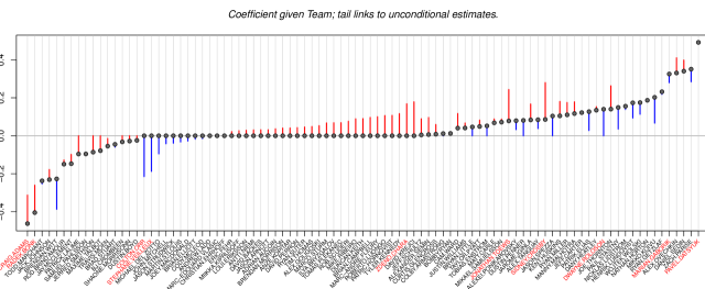
Observe that incorporating team effects causes many more player effects to be zeroed out, with many players’ stand-out performance being absorbed by their respective teams (red lines tracking to zero). Note that ability estimates for players who frequently share the ice will generally be negatively correlated: if players are always on the ice together when a goal is scored, an increase in the estimated effect of one player must be accompanied by a decrease in the effect of the other player. In MAP estimation under a sparsity-inducing L1 penalty, this will often manifest itself by forcing one player’s effect being estimated at zero.

Perhaps the most surprising result is that Sidney Crosby, considered by many to be the best player in the NHL, has a contribution that drops after accounting for his team (although he still stands out). Jonathan Toews’ and Zdeno Chara’s effects show similar behavior, the latter having no player–team effect. As all three players captain their respective (consistently competitive) teams, we should perhaps not be surprised that team success is so tightly coupled to player success in these cases.

An exception is Pavel Datsyuk, who stands out as the leagues very best, having a coefficient that is unmoved even after considering the strong team effect of his Red Wings. There are also a few players, such as Dwayne Roloson, who shine despite their team. Roloson has a strong positive effect in the player–team model but a null one in the player-only model. We will revisit this particular result in Section 3.2.

On the negative side, Colton Orr and Stephane Veilleux seem to shoulder undue blame for their team’s poor performance. Orr, recognized as an enforcer when on the ice, may not have been used effectively by his coaching staff. Veilleux played alongside Gaborik on the Wild in the late 2000s, and both players get a positive bump in the player–team model. Finally, Craig Adams and Radek Bonk stand out as poor performers in both models.

3.2 Comparison to traditional plus-minus

Our variable selection approach provides a rich but compact summary of player performance. In our team-player model with an L1 penalty, the vast majority of players obtain a “mediocre” $\hat{\beta}_{j}=0$ and our focus can be narrowed to those who have a significant partial effect on scoring. In contrast, plus-minus assigns a non-zero number for most players without any reference to statistical significance. Thus the most obvious departure from traditional plus-minus is that far fewer players are distinguishable from their team-average under our performance metric.

From the model equation in (1), nonzero partial player estimates are an additive effect on the log odds that, given a goal has been scored, it is a goal for that player’s team (controlling for team and the other players). In other words, $e^{\beta_{j}}$ is a multiplier on the for-vs-against odds for every goal where player $j$ is on the ice, so that our parameters $\beta$ relate multiplicatively to the ratio of for-vs-against, while traditional plus-minus is calculated as the difference between for-vs-against goals. Moreover, our partial effects measure deviations in performance from the team average so that a player on a very good team needs to be even better than his teammates to gain a positive $\beta$, while an average player on a good team has an impressive plus-minus measure just by keeping up.

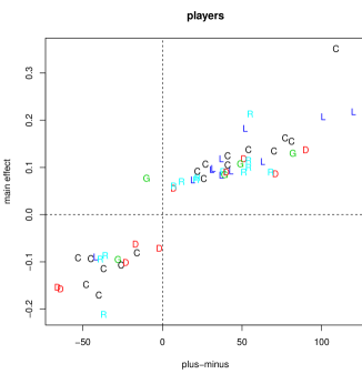
Despite these differences, both metrics are an attempt to quantify player contribution. Figure 3 compares our MAP estimates of player partial effects from the team-player model to the traditional plus-minus aggregated over our four seasons of data. The left-hand plot shows the player estimates, labeled by positional information.

team	MAP	$+/-$
T.B	$-0.165$	$-159$
NYI	$-0.126$	$-143$
EDM	$-0.077$	$-103$
ATL	$-0.045$	$-80$
COL	$-0.025$	$-60$
OTT	$-0.020$	$-56$
MIN	$-0.019$	$-52$
TOR	$-0.017$	$-70$
NSH	$0.019$	$9$
S.J	$0.045$	$93$
BOS	$0.103$	$109$
CHI	$0.106$	$99$
PIT	$0.112$	$114$

Figure 3: Left: Comparing plus-minus, aggregated over the four seasons considered in our analysis, to the MAP partial effects $\hat{\beta}$. Plot symbols give positional information: C = center, L = left wing, R = right wing, D = defense, and G = goalie. Right: Comparing team partial effects $\hat{\alpha}$ to their plus-minus values.

Discrepancies between the two metrics in Figure 3 are informative. One player, Dwayne Roloson, has a plus-minus whose sign disagrees with that on his $\hat{\beta}_{j}$. We also noted earlier that Roloson has a partial player effect that is pulled up in the team–player model compared to the player-only model. For an explanation, we can examine the $\hat{\alpha}_{j}$ coefficients of the teams which appear in the table on the right-panel of Figure 3. Each of the four teams Roloson played for (T.B, NYI, EDM, and MIN) all have significantly negative $\hat{\alpha}_{j}$ values. Apparently Roloson was a quantifiable star on a string of poorly performing teams. Our model reasonably attributes many of the goals counting against him in his traditional plus-minus as counting against his team as a whole.

Another observation from Figure 3 is that our model estimates disagree with traditional plus-minus about who is the best player in hockey. Alex Ovechkin is the player with the largest plus-minus value, although there are nearly a dozen other players with plus-minus values are within ten percent of his. In contrast, Pavel Datsyuk is the best player according to our partial player effects by a huge margin: his posterior odds of contributing to a goal for his team are nearly 50% larger than the next best players (Ovechkin and Gaborik).

The second best player in hockey by traditional plus-minus is Roberto Luongo. However, from Figure 2, we see that Luongo’s partial player estimate is $\hat{\beta}_{j}=0$. In the context of a goalie, the implication is that his play is not significantly different from that of his back-ups on the Vancouver Canucks. This suggests that undue blame and credit may have been placed on Luongo for both regular season successes and postseason collapses. At the other end, observe that the best ranked player with a negative partial player estimate (Michael Del Zotto) has a nearly-zero plus-minus value.

3.3 Prior sensitivity analysis

MAP estimates for each $\beta_{j}$ are sensitive to $\mathrm{E}[\lambda_{j}]$, the expected L1 penalty for each coefficient. This relationship is illustrated in Figure 4, which shows estimated coefficients under increasing penalty for some players with large effects in Sections 3.1-2. We see that as the expected value of the penalty term grows, the number of non-zero players (top X-axis of Figure 4) decreases substantially, which illustrates the variable selection aspect of our model. The magnitudes of the MAP estimates of partial player effects $\beta_{j}$ are also shrunk towards zero with larger penalties.

Figure 4: Coefficient estimates for a subset of players (chosen from all players with nonzero coefficients at $\mathrm{E}[\lambda_{j}]=15$, our specification in Sections 3.1-2). The expected L1 penalty is shown along the bottom, with corresponding % of estimated $\beta_{j}\neq 0$ along the top and coefficient value on the right.

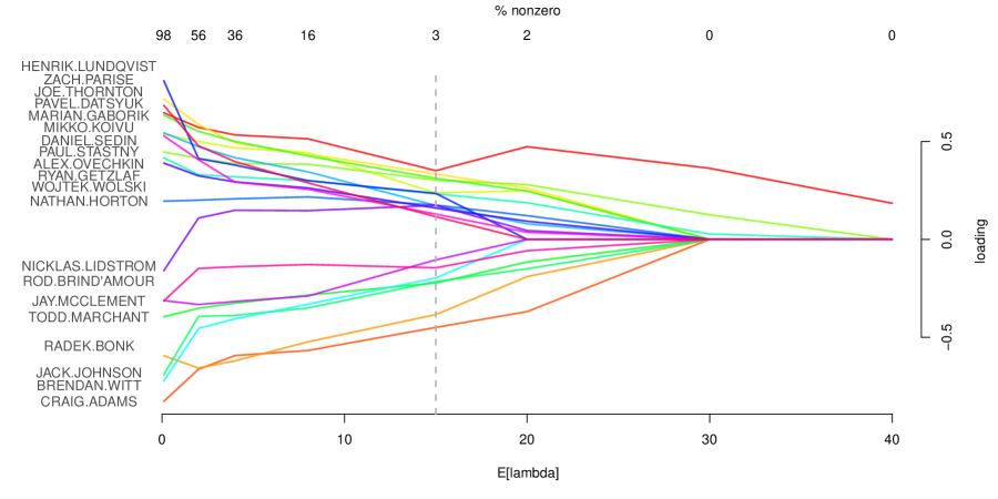
The far left values have a very low $\mathrm{E}[\lambda_{j}]=1/10$ and non-zero $\hat{\beta}_{j}$ for 98% of players. At this extreme, there are three plotted players with stronger effect than Datsyuk. Only Zach Parise is more effective than Datsyuk at $\mathrm{E}[\lambda_{j}]=2$, which leads to 56% of players with non-zero effects. At $\mathrm{E}[\lambda_{j}]=4$, Datsyuk is the top player and 36% of players have non-zero effects. Datsyuk remains the best player at very high penalization levels, until he is the only measurable contributor in the league.

More dramatic changes can be found in the (un-plotted) estimates for players with relatively low ice-time. As an example, Michel Ouellet is among the top estimated performers in the league for $\mathrm{E}[\lambda_{j}]<10$, but he jumps to a zero $\hat{\beta}_{j}$ under higher penalties. Given this sensitivity, it is worth revisiting hyperprior specification. Although we have chosen $\mathrm{E}[\lambda_{j}]$ with help from results of Section 4, this value was also only slightly higher than where non-star players (e.g., Ouellet) drop out of the top $\hat{\beta}_{j}$ rankings. In the absence of reliable out-of-sample testing, one pragmatic option is to increase penalty until the results become unrealistic. Similarly, one can interpret estimates conditional on the number of nonzero coefficients, and consider the $\hat{\beta}_{j}$ as performance measured under a given level of sparsity. A better approach, however, is to nearly eliminate sensitivity to the prior by averaging over penalty uncertainty, as we do in Section 4.

3.4 Value for money

In the left of Figure 5, we plot MAP $\hat{\boldsymbol{\beta}}$ estimates from our model versus 2010-11 salaries for the non-zero coefficients. Plus-minus points (rescaled to fall into the same range) have also been added to the left plot.

Figure 5: The left plot shows non-zero MAP $\hat{\boldsymbol{\beta}}$ estimates versus 2010-11 salary, augmented with rescaled plus-minus points for comparison. Ordinary least squares fits are added to aid in visualization. The right plot shows the histogram of 2010-11 salaries for players with $\hat{\beta}_{j}=0$, extending to the full set in gray.

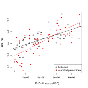
The lines overlaid on the left plot are ordinary least squares fits for each metric; a hypothesis test for the interaction coefficient reveals that indeed the two lines differ (at the 5% level; $p=0.026$). Since the $\beta_{j}$ relate to performance on a log scale, as is typically assumed for salary, we are not surprised to see a linear relationship between salary and our player effects. The fact that the standard errors for the $\hat{\boldsymbol{\beta}}$ fit (0.1226) is less than the plus-minus fit (0.1605) with the same design inputs suggests that our model-based player effects $\hat{\boldsymbol{\beta}}$ have greater correlation to player salary. Teams appear to be compensating their players using strategies that are more in line with our partial player effects ($\boldsymbol{\beta}$) than with traditional plus-minus.

One reason why our model estimates have a lesser slope with salary is that fewer players are estimated to have a substantial (non-zero) negative contribution by our model compared to traditional plus-minus. Despite the decent correlation between our model estimates and player salary, it is also clear that there are some mis-priced players. The best player according to our model, Pavel Datsyuk, probably deserves a raise whereas Sidney Crosby may be somewhat over-priced. Alex Ovechkin seems to be correctly priced in the sense that he is close to the fitted line between his model estimate and his salary.

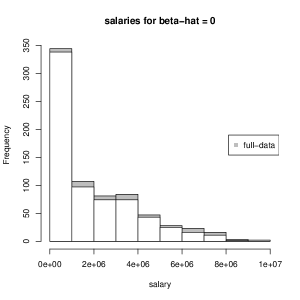
In the right of Figure 5, we give the salary distribution for players that were estimated to have zero player effects. Clearly, there are many players with high salaries but which are estimated by our model to not have a substantial player effect. Specifically, the top ten salaries for players with $\hat{\beta}_{j}=0$ are Chris Pronger ($7.6M), Henrik Zetterberg ($7.75M), Brad Richards ($7.8M), Marian Hossa ($7.9M), Chris Drury ($8M), Scott Gomez ($8M), Duncan Keith ($9M), Evgeni Malkin ($10M), and Vincent Lecavalier ($10M).

The gray extensions to the histogram indicate the full salary distribution, including players where $\hat{\beta}_{j}\neq 0$. With the exception of the bins containing the largest salaries, the absolute tally of $\hat{\beta}_{j}\neq 0$ players is fairly uniform. It is somewhat surprising that a relatively large proportion of top-dollar players find themselves with player effects of zero.

4 Full Posterior Estimation and Decision Making

The full posterior distribution from our penalized logistic regression model was estimated via Markov-Chain Monte Carlo simulation, with details given in Appendix A. We will first use the full posterior distribution to re-examine our player effects $\beta_{j}$ while accounting for possible covariance between players. We will then consider additional salary information to explore optimal line combinations and matchups under budget constraints in Section 4.2. Neither of these analyses is possible without samples from the full posterior distribution.

4.1 Posterior Analysis of Team–player Model

In contrast with the MAP estimates from Section 3, samples from the full posterior distribution do not easily emit a variable selection. However, these posterior samples do contain much richer information about relative player ability via the covariance structure of the $\boldsymbol{\beta}$. One way of analyzing this information is by constructing a matrix with the posterior probability that each player is better than every other player. Specifically, for each player pair $(i,j)$, we calculate the proportion of samples where $\beta_{i}^{(t)}$ is larger than $\beta_{j}^{(t)}$.

As an example, Figure 6 shows three players (Datsyuk, Roloson, and Marchant), pitting each of them against the 90-odd players with non-zero MAP estimates under the team–player model. Comparisons under both the team–player and player-only models are provided. Note that the $x$-axis has been slightly re-ordered by the posterior mean in the team–player model to make the corresponding curves smoother.

Figure 6: Comparing the ability of Datsyuk (black), Roloson (red), and Marchant (green) to the 90-odd other players with non-zero coefficients in either the team–player or player-only models. These three players are also indicated in red among the list of players on the X-axis. Thicker lines correspond to the team–player model.

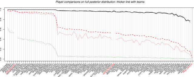
Observe how Roloson’s curves indicate a large discrepancy under the team-player and player-only models (since he played well with poor teams), whereas Datsyuk’s and Marchant’s show negligible differences. We are not aware of any other player effect that can be examined (pairwise or otherwise) at this resolution, and on such readily-interpretable probabilistic terms.

4.2 Posterior Player Match-ups and Line Optimization

Beyond examining pairwise differences, another way to explore our full posterior results is through match-ups and line combinations based on the posterior predictive distribution that accounts for covariances among our set of players. Later, we will also build in external constraints in the form of a cap on salaries.

Specifically, we will calculate the posterior probability that one particular configuration of players (line A) is more likely to score or be scored upon when facing another configuration (line B). This type of calculation would allow coaches to explore specific line match-ups against opponents. In these match-ups, team information will be ignored but position information respected: we construct only six-on-six match-ups with one goalie, center, left-wing, right-wing, and two defensemen on each side.

Consider the following four analyses, where we use our posterior results to either: 1. pit the best players against the worst players, 2. pit the best players against random players, 3. pit random players against the worst players, and 4. pit random players against other random players. When pitting the best against the worst we construct the input $x^{(t)}$ for each sample $\boldsymbol{\beta}^{(t)}$ as follows. Place $1$’s in slots for players in each position with the largest $\boldsymbol{\beta}^{(t)}$ value, and $-1$’s in those with the smallest (largest negative) value. Fill the rest of the components with zeros. Then, a sample from the probability that the best team (regarded as the “offense”) scores is calculated by ${\rm P}({\rm``offense"}\,{\rm scores})=\mathrm{logit}(x^{(t)\top}\boldsymbol{\beta}^{(t)})$ . A comparison of best versus random, worst versus random or random versus random would proceed similarly where the random sampling is without replacement.

Figure 7: Posterior probability that “offense” scores in various line matchups (smoothed using a kernel density). Better team (listed first) is always considered to be the offense.

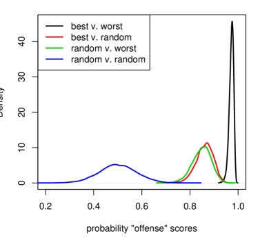
Figure 7 shows the results of these matchups, where the distribution of posterior probabilities that the offense scores are smoothed using a kernel density. It is reassuring to see that offense lines consisting of the best players have a very high probability of scoring on the worst players and with very low variance. This is indicative of a strong signal distinguishing good from bad players in the data. Likewise, it is not surprising that the random players outscore their random counterparts about half the time, and with high uncertainty. What is interesting is that the “best v. random” and “random v. worst” densities are not the same: there is a small but clear indication in the posterior distribution that the worst players hurt more than the best players help.

An extended analysis incorporating salary information paints are more provocative picture. We now construct our line match-ups subject to a salary budget/cap $B$, by solving the following binary program:

$$\max_{x\in\{0,1\}^{n_{p}}} x^{\top}\boldsymbol{\beta}^{(t)},$$

$$\mbox{subject to}\;\;\;x^{\top}s \leq B$$ (4)

$$\mbox{and}\;\;\;\;x^{\top}g =1,\;\;x^{\top}\ell=1,\;\;x^{\top}r=1,\;\;x^{\top}d=2,$$

where $s$ is an $n_{p}$-vector of player salaries, and $(g,c,l,r,d)$ are $n_{p}$-vectors of binary indicators for goalies, centers, wingers and defensemen, respectively, so that player positions are still respected. The argument of each solution $x^{(t)}$ obtained from the binary program is then mapped to a posterior sample of the player effects $\beta^{(t)}$, which gives us the posterior probability $\mathrm{logit}(x^{(t)\top}\beta^{(t)})$ that the line scores against a random opponent.

Figure 8: The left panel shows kernel density plots of the probability that an optimally chosen line scores against a random line according to the full posterior distribution of $\beta$ and under several salary caps; the right panel shows the means and 90% predictive intervals of the same posterior as a function of those caps.

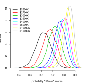
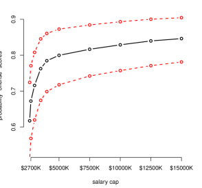
The left panel of Figure 8 shows the distribution of the probability the offense scores for several values of $B$ spanning from $2.6 million (0.26 $\times$ the current maximum salary of $10 million) to $15 million. The right panel shows the posterior means and 90% credible intervals for the probability that the offense scores as a function of the budget. The first observation is that there is tremendous value amongst the cheapest players. Lines can be formed among the cheapest players which still outscore their (random) opponents 65% of the time, on average. Importantly, the posterior probability that this quantity is bigger than 50% (i.e., that the best low paid players are better than random ones) is 0.98. A second observation is that lines formed without the most expensive players, i.e., with a budget less than ($10M), are only marginally worse than those which have these most expensive players. This means that the most expensive players may not be good value for money, at least as far as scoring goals. Having the capacity to have two of the most expensive players on the ice at once (e.g., Crosby and Malkin for the Penguins) seems to offer no advantage at all.

Inspecting the individual players that are involved in these optimal lines in each budget category is also revealing. Brian Boucher, a goalie for the Flyers, is extremely valuable for the money, costing just $92.5K. He is the most frequently selected player for each of the four lowest budgets ($2.6-3.5M). Al Montoya ($750K) is in the top five of choices in all budgets above the lowest four, representing a cheap but solid filler player that allows more budget to be allocated to expensive stars. At very the top end, Pavel Datsyuk ($6.7M) is unsurprising good value for the top three budgets ($10-15M). Ovechkin comes in at a respectable 20^th place among all players despite his high cost ($9M). Crosby (also $9M) comes in the top 25%. The most expensive players, Lecavalier and Luongo, are not selected often at all, suggesting that money is better spent on cheaper (and younger) talent.

5 Discussion

In this paper, we use a logistic regression model to estimate the effects of individual players on goal scoring in hockey. Unlike the traditional plus-minus measure that is commonly used, our player effects account for the match-ups involved in each goal as well as overall team contributions.

We take a Bayesian approach with a prior distribution that shrinks the coefficients towards zero, which promotes stability in our model and protects against over-fit. The Laplace prior distribution placed on the individual player coefficients allows us to perform variable selection on the large scale needed for this data situation. With this variable selection, we are able to separate out a small subset of players that show substantially above-average performance.

Our analysis gives some surprising results, such as the dominance of Pavel Datsyuk over other star players such as Sidney Crosby and Alex Ovechkin. We also find that several prominent players, such as Evgeni Malkin, do not have significant player effects.

The point estimates $\hat{\boldsymbol{\beta}}$ and samples from the full posterior distribution offer insight into relative player ability at a resolution not previously available. Such partial effects and pairwise comparisons are new metrics derived from making better use of the same data source behind plus-minus, obtained by leveraging newfound computational tractability in high dimensional logistic regression modeling. We show in our appendix that it is possible to entertain player–player interaction effects too, although ultimately conclude that these offer little further insight.

By introducing outside data sources, such as player salary information and constraints thereon (i.e., salary budgets), our approach offers unprecedented potential for exploratory analysis, tinkering, and ultimately decision making by coaches, general managers, and fantasy players alike. This analysis of match-ups would only be possible with our fully Bayesian approach that accounts for the covariance between individual player effects by using samples from the joint posterior distribution.

A more believable model for the combination of shift timings and goals would be to treat every game as a Poisson point process, where each goal is a point-event and the expected time between goals depends upon who is on the ice. However, such an approach requires restrictive modeling assumptions and considerably more computation, and we doubt that the value of information about when goals were not scored is worth the added complexity. The popularity of traditional plus-minus is informative: player ability can be measured from the subset of events that actually lead to goals. Thus while not completely discounting the potential of time-dependent modeling, we present the work herein as a robust analysis that is replicable, extensible, and based upon easily available data. Similarly, we have not used power play or short-handed goals in our analysis, but extending our model to non-even-strength situations is a promising direction for future work.

Acknowledgments

Many thanks to Samuel Ventura and Andrew C. Thomas for supplying a cleaned version of the nhl.com data. We are grateful to the editor, an associate editor, and one referee whose comments on an early version of the manuscript led to many improvements.

Appendix

Appendix A Estimation Details and Software

Although L1 penalty methods and their Bayesian interpretation have been known for some time, it is only recently that joint penalty–coefficient posterior computation and simulation methods have become available for datasets of the size encountered here.

Probably the most well-known publicly available library for L1 penalty inference in logistic regression is the glmnet package (Friedman et al.,, 2010) for R. Conditional on a single shared value of $\lambda$, this implementation estimates a sparse set of coefficients. A convenient wrapper routine called cv.glmnet allows one to chose $\lambda$ by cross-validation (CV). Unfortunately, CV works poorly in our setting of large, sparse, and imbalanced $X_{P}$, where each model fit is relatively expensive and there is often little overlap between nonzero covariates in the training and validation sets. Moreover, when maximizing (rather than sampling from) the posterior, a single shared $\lambda$ penalty leads to over-shrinkage of significant $\beta_{j}$ as penalty choice is dominated by a large number of spurious predictors. But use of CV to choose unique $\lambda_{j}$ for each covariate would imply an impossibly large search.

Instead, we propose two approaches, both accompanied by publicly available software in packages for R: joint MAP inference with textir, and posterior simulation with reglogit.

A.1 Fast variable selection and MAP inference with textir

Taddy, (2013) proposes a gamma-lasso framework for MAP estimation in logistic regression, wherein coefficients and their independent L1 penalties are inferred under a conjugate gamma hyperprior. An efficient coordinate descent algorithm is derived, including conditions for global convergence, and the resulting estimation is shown in Taddy, (2013) as superior, in both predictive performance and computation time, to the more common strategy of CV lasso estimation under a single shared $\lambda$ (as in glmnet). Results in this paper were all obtained using the publicly available textir package for R (Taddy,, 2012), which uses the slam (Hornik et al.,, 2011) package’s simple-triplet matrices to take advantage of design sparsity.

Prior specification in the gamma-lasso attaches independent gamma $\mathrm{G}(\lambda_{j};s,r)$ hyperpriors on each L1 penalty, with $\mathrm{E}[\lambda_{j}]=s/r$ and $\mathrm{var}[\lambda]=s/r^{2}$, such that, for $j=1\ldots p$,

$$\pi(\beta_{j},\lambda_{j})=\mathrm{Laplace}(\beta_{j};\lambda_{j})\mathrm{G}(\lambda_{j};s,r)=\frac{r^{s}}{2\Gamma(s)}\lambda_{j}^{s}e^{-\lambda_{j}\left(|\beta_{j}|+r\right)},~{}~{}s,r,\lambda_{j}>0.$$ (5)

Laplace priors are often motivated through estimation utility—the prior spike at zero corresponds to a preference for eliminating regressors from the model in absence of significant evidence. Our hyperprior is motivated by complementary considerations: for strong signals and large $|\beta_{j}|$, expected $\lambda_{j}$ shrinks in the joint distribution to reduce estimation bias.

This leads to the joint negative log posterior minimization objective

$$l(\boldsymbol{\alpha},\boldsymbol{\beta})=\sum_{i=1}^{n_{g}}\log\left(1+\exp\left[-y_{i}(\mathbf{x}_{Ti}^{\prime}\boldsymbol{\alpha}+\mathbf{x}_{Pi}^{\prime}\boldsymbol{\beta})\right]\right)+\frac{1}{2\sigma^{2}}\sum_{t=1}^{30}\alpha_{t}^{2}+\sum_{j=1}^{n_{p}}s\log(1+|\beta_{j}|/r),$$ (6)

where $s$, $r$ $>0$. We have set $\sigma=1$ and $r=1/2$ throughout Section 3. In choosing $s=\mathrm{E}[\lambda_{j}]/2$, we focus on the conditional prior standard deviation, ${\rm SD}(\beta_{j})=\sqrt{2}/\lambda_{j}$, for the coefficients. Hence our value of $s=7.5$, for $\mathrm{E}[\lambda_{j}]=15$, implies expected ${\rm SD}(\beta_{j})\approx 0.095$. To put this in context, $\exp[3\times 0.095]\approx 1.33$, implying that a single player increasing his team’s for-vs-against odds by $1/3$ is 3 deviations away from the prior mean.

As an illustration of the implementation, the following snippets show commands to run our main team–player model (see ?mnlm for details). With X = cbind(XP,XT) as defined in Section 2.1, the list of 30 ridge and $n_{p}$ gamma-lasso penalties are specified

pen <- c(rep(data.frame(c(0,1)),30),rep(data.frame(c(7.5,.5)),ncol(XP)))

and the model is then fit

fit <- mnlm(counts=Y, covars=X, penalty=pen, normalize=FALSE)

where X is not normalized since this would up-weight players with little ice-time.

A.2 Full posterior inference via reglogit

Extending a well-known result by Holmes and Held, (2006), Gramacy and Polson, (2012) showed that three sets of latent variables could be employed to obtain sample from the full posterior distribution using a standard Gibbs strategy (Geman and Geman,, 1984). The full conditionals required for the Gibbs sampler are given below for the L1 and $\lambda_{j}=\lambda$ case (note that $\boldsymbol{\beta}$ includes $\boldsymbol{\alpha}$ here for notational convenience).

$$\boldsymbol{\beta}|z,\tau^{2},\omega,\lambda \sim\mathcal{N}_{p}(\tilde{\boldsymbol{\beta}},V) \tilde{\boldsymbol{\beta}} =V(y.X)^{\top}\Omega^{-1}z,\;y.X\equiv\mathrm{diag}(y)X$$

$$\lambda|\boldsymbol{\beta} \sim\mathrm{G}\left(a+p,b+\sum_{j=1}^{p}|\beta_{j}|\right) V^{-1} =\lambda^{2}\Sigma^{-1}D_{\tau}^{-1}+(y.X)^{\top}\Omega^{-1}(y.X)$$

$$\tau_{j}^{-2} \sim\mbox{Inv-Gauss}(|\lambda/\beta_{j}|,\lambda^{2}), j =1,\dots,p\equiv\mathrm{ncol}(X)$$

$$z_{i}|\boldsymbol{\beta},\omega_{i},y_{i}, \sim\mathcal{N}^{+}\!\left(y_{i}x_{i}^{\top}\boldsymbol{\beta},\omega_{i}\right), i =1,\dots,n\equiv\mathrm{length}(y).$$

$$\omega_{i}|y_{i},\lambda \sim\mbox{See below} i =1,\dots,n$$

Note that $\mathcal{N}^{+}$ indicates the normal distribution truncated to the positive real line, $D_{\tau}=\mathrm{diag}(\tau_{1}^{2},\dots,\tau_{p}^{2})$ and $\Omega=\mathrm{diag}(\omega_{1},\dots,\omega_{n})$. Holmes and Held, (2006) give a rejection sampling algorithm for $\omega_{i}|z_{i}$, however Gramacy and Polson, (2012) argue that it is actually more efficient to draw $\omega_{i}|y_{i},\lambda$ (i.e., marginalizing over $z_{i}$) as follows. A proposal $\omega_{i}^{\prime}=\sum_{k=1}^{K}2\psi_{k}^{-1}\epsilon_{k}$, and $\epsilon_{k}\sim\mathrm{Exp}(1)$ may be accepted with probability $\min\{1,A_{i}\}$ where $A_{i}=\Phi\{(-y_{i}x_{i}^{\top}\boldsymbol{\beta})/\sqrt{\omega_{i}^{\prime}}\}/\Phi\{(-y_{i}x_{i}^{\top}\boldsymbol{\beta})/\sqrt{\omega_{i}}\}$. Larger $K$ improves the approximation, although $K=100$ usually suffices. Everything extends to the L2 case upon fixing $\tau_{j}^{2}=1$. Extending to separate $\lambda_{j}$ is future work.

We use the implementation of this Gibbs sampler provided in the reglogit package (Gramacy,, 2012a) for R. For the $\lambda$ prior we use the package defaults of $a=2$ and $b=0.1$ which are shared amongst several other fully Bayesian samplers for the ordinary linear regression context (e.g., blasso in the monomvn package (Gramacy,, 2012b)). Usage is similar to that described for mnlm. To obtain T samples from the posterior, simply call:

bfit <- reglogit(T=T, y=Y, X=X, normalize=FALSE)

Estimating the full posterior distribution for $\boldsymbol{\beta}$ allows posterior means to be calculated, as well as component-wise variances and correlations between $\beta_{j}$’s. However, unlike MAP estimates $\hat{\boldsymbol{\beta}}$, none of the samples or the overall mean is sparse. Gramacy and Polson, (2012) show how their algorithm can be extended to calculate the MAP via simulation, but this only provides sparse estimators in the limit.

Another option is to use the posterior mean for $\lambda$ obtained by Gibbs sampling on the entire covariate set, and use it as a guide in MAP estimation. Indeed, this is what is done in Section 3, where mean of our shared $\lambda$ from Gibbs sampling was considered when setting setting priors for $\mathrm{E}[\lambda_{j}]$.

Appendix B Extension to player–player interactions

We explore the possibility of on-ice synergies or mismatches between players by adding interaction terms into our model. The extension is easy to write down: simply add columns to the design matrix that are row-wise products of unique pairs of columns in the original $X_{P}$. However, this implies substantial computational cost: see Gramacy and Polson, (2012) for examples of regularized logistic regression estimators that work well for estimating main effects but break down in the presence of interaction terms.

There is a further representational problem in the context of our hockey application. There are about 27K unique player pairs observed in the data. Combining these interaction terms with the original $n_{p}$ players, $n_{g}$ goals and thirty teams, we have a double-precision data storage requirement of nearly a gigabyte. While this is not a storage issue for modern desktops, it does lead to a computational bottleneck since temporary space required for the linear algebra routines cannot fit in fast memory. Fortunately, our original design matrix has a high degree of sparsity, which means that the interaction-expanded design matrix is even more sparse, and the sparse capabilities of textir makes computation feasible. Inference on the fully interaction-expanded design takes about 20 seconds on an Apple Mac Desktop. All other methods we tried, including reglogit, failed in initialization stages.

Figure 9: Comparing (non-zero) main effects for team–player model to their values in the interaction-expanded team–player model (dots) The lines point to the unexpanded estimates, and the $x$-axis is ordered by the dots.

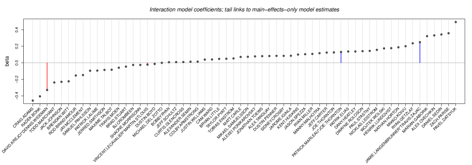
While the computational feat is impressive, our results indicate little evidence of significant player interaction effects. Figure 9 shows results for estimation with $\mathrm{E}[\lambda=15]$: only four non-zero interactions are found when augmenting the team–player model to include player–player interaction terms. Importantly, there is a negligible effect of including these interactions on the individual player effect estimates (which are our primary interest). The only player with a visually detectable connecting line is Joe Thornton, and to see it you may need a magnifying glass. We guess from the neighboring interaction term that his ability is enhanced when Patrick Marleau is on the ice. The most interesting result from this analysis involves the pairing of David Krejci and Dennis Wideman, which has a large negative interaction. One could caution Bruins coach Claude Julien against having this pair of players on the ice at the same time.

Using reglogit to obtain samples from the full posterior distribution of the interaction-expanded model is not feasible, but we can still glean some insight by sampling from the posterior distribution for the simpler model with the original team-player design augmented to include the four significant interactions found from our initial MAP analysis.

Figure 10: Comparing the ability of Datsyuk, Roloson, and Marchant to the 60-odd other players with non-zero coefficients in the team–player model, showing coefficients under the interaction-expanded model as well.

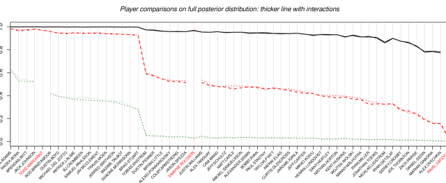
Figure 10 compares pairwise abilities for the same three players used as examples in Figure 6. We observe minimal changes to the estimates obtained under the original team–player design, echoing the results from the MAP analysis. In total, we regard the ability to entertain interactions as an attractive feature of our methodology, but it does not change how we view the relative abilities of players.

References

- Awad, (2009) Awad, T. (2009). “Numbers On Ice: Fixing Plus/Minus.” Hockey Prospectus, April 03, 2009.
- Friedman et al., (2010) Friedman, J. H., Hastie, T., and Tibshirani, R. (2010). “Regularization Paths for Generalized Linear Models via Coordinate Descent.” Journal of Statistical Software, 33, 1, 1–22.
- Geman and Geman, (1984) Geman, S. and Geman, D. (1984). “Stochastic relaxation, Gibbs distributions, and the Bayesian restoration of images.” IEEE Transaction on Pattern Analysis and Machine Intelligence, 6, 721–741.
- Gramacy, (2012a) Gramacy, R. (2012a). reglogit: Simulation-based Regularized Logistic Regression. R package version 1.1.
- Gramacy and Polson, (2012) Gramacy, R. and Polson, N. (2012). “Simulation-based Regularized Logistic Regression.” Bayesian Analysis, 7, 1–24.
- Gramacy, (2012b) Gramacy, R. B. (2012b). monomvn: Estimation for multivariate normal and Student-t data with monotone missingness. R package version 1.8-9.
- Hoerl and Kennard, (1970) Hoerl, A. E. and Kennard, R. W. (1970). “Ridge regression: biased estimation for nonorthogonal problems.” Technometrics, 12, 55–67.
- Holmes and Held, (2006) Holmes, C. and Held, K. (2006). “Bayesian Auxilliary Variable Models for Binary and Multinomial Regression.” Bayesian Analysis, 1, 1, 145–168.
- Hornik et al., (2011) Hornik, K., Meyer, D., and Buchta, C. (2011). slam: Sparse Lightweight Arrays and Matrices. R package version 0.1-23.
- Ilardi and Barzilai, (2004) Ilardi, S. and Barzilai, A. (2004). “Adjusted Plus-Minus Ratings: New and Improved for 2007-2008.” 82games.com.
- Macdonald, (2010) Macdonald, B. (2010). “A Regression-based Adjusted Plus-Minus Statistic for NHL Players.” Tech. rep., arXiv: 1006.4310.
- Rosenbaum, (2004) Rosenbaum, D. T. (2004). “Measuring How NBA Players Help Their Teams Win.” 82games.com, April 30, 2004.
- Schuckers et al., (2010) Schuckers, M. E., Lock, D. F., Wells, C., Knickerbocker, C. J., and Lock, R. H. (2010). “National Hockey League Skater Ratings Based upon All On-Ice Events: An Adjusted Minus/Plus Probability (AMPP) Approach.” Tech. rep., St. Lawrence University.
- R Development Core Team, (2010) R Development Core Team (2010). R: A Language and Environment for Statistical Computing. R Foundation for Statistical Computing, Vienna, Austria. ISBN 3-900051-07-0.
- Taddy, (2012) Taddy, M. (2012). textir: Inverse Regression for Text. R package version 1.8-6.
- Taddy, (2013) — (2013). “Multinomial Inverse Regression for Text Analysis.” Journal of the American Statistical Association, to appear.
- Thomas et al., (2012) Thomas, A. C., Ventura, S. L., Jensen, S., and Ma, S. (2012). “Competing Process Hazard Function Models for Player Ratings in Ice Hockey.” Tech. rep., ArXiv:1208.0799.
- Tibshirani, (1996) Tibshirani, R. (1996). “Regression shrinkage and selection via the lasso.” J. R. Statist. Soc. B, 58, 267–288.
- Vollman, (2010) Vollman, R. (2010). “Howe and Why: Ten Ways to Measure Defensive Contributions.” Hockey Prospectus, March 04, 2010.