A Bayesian Nonparametric Approach to Image Super-resolution

Abstract

Super-resolution methods form high-resolution images from low-resolution images. In this paper, we develop a new Bayesian nonparametric model for super-resolution. Our method uses a beta-Bernoulli process to learn a set of recurring visual patterns, called dictionary elements, from the data. Because it is nonparametric, the number of elements found is also determined from the data. We test the results on both benchmark and natural images, comparing with several other models from the research literature. We perform large-scale human evaluation experiments to assess the visual quality of the results. In a first implementation, we use Gibbs sampling to approximate the posterior. However, this algorithm is not feasible for large-scale data. To circumvent this, we then develop an online variational Bayes (VB) algorithm. This algorithm finds high quality dictionaries in a fraction of the time needed by the Gibbs sampler.

I Introduction

The sparse representation of signals with a basis is important in many applications. It has been extensively used in image denoising, inpainting, super-resolution, classification and compressive sensing [1, 2, 3, 4, 5, 6, 7, 8].

Many real data sets can be sparsely represented in some basis; typically this basis itself has to be learned from the data [1, 2, 3, 6, 7, 8, 9, 10, 11, 12]. For example, an image can be represented by weighted combinations of recurrent patterns of pixels. This construction may be beneficial, both while building a model for more accurate representation of the data (e.g. superior image denoising models) and while deriving and implementing an inference procedure for more efficient algorithms.

In this paper we consider image super-resolution (SR), the problem of recovering a high-resolution (HR) image from a low-resolution (LR) image. It has many applications, e.g., to smart phones, surveillance cameras, medical imaging, and satellite imaging.

There are a variety of approaches for image super-resolution. In general, rendering an HR image from an LR image has many possible solutions. We must use regularization of some form, i.e., prior information about the HR, to guarantee uniqueness and stability of the extension. For this purpose, researchers have proposed several methods [13, 14]. Interpolation-based methods, such as the Bicubic method and Bilinear method, often over-smooth images, losing detail. Example-based approaches use machine learning to avoid this [15, 16, 17]; they train on ground-truth HR and LR images, learning a statistical relationship between the two. These relationships are later used to reconstruct unknown HR images from corresponding LR images. Freeman et al. ([15]) proposes a method that stores a training set of preprocessed patches and uses a nearest-neighbor search to super-resolve. Kim et al. ([16]) proposes using kernel ridge regression with a regularized gradient descent. Another class of SR algorithms use texture similarity to match image regions with known textures [18, 19]. Finally, there are methods for single-image super-resolution. One classic example is [20] which uses recurring patterns at same and different scales in a single image.

In this work, our focus is on SR via example-based sparse coding. ScSR (Super-resolution via Sparse Representation) is such an algorithm pioneered in [21]. This algorithm is based on sparse coding via L1 regularized optimization. In [21], image data are represented using a collection of dictionary elements (recurring patterns of pixels) that are weighted across different positions. Although very powerful, this model requires one to specify the number of dictionary elements and the variance of the noise model in advance—parameters that may be difficult to assess for real-world images. It also only provides a batch learning algorithm, i.e., computing model parameters via a gradient descent algorithm on a fixed small subset of the data.

Bayesian nonparametric methods circumvent all these limitations. These methods adapt the structure of the latent space to the data and provide a powerful representation because they infer parameters that otherwise have to be assigned a priori [22, 23, 24, 25, 26, 27, 28, 29, 30, 31, 32]. The full posterior distribution can be approximated via MCMC or variational inference, yielding sparse representations and learned dictionaries.

Bayesian nonparametric methods have been used in many image analysis applications: to learn deep architectures used for object recognition in [22], for image inpainting and denoising in [28, 29], for image segmentation in [30, 31], and to learn nonparametric multiscale representations of images in [32].

In this paper, we develop a Bayesian nonparametric method for super-resolution. We show that inference in our model is feasible, performing super-resolution with both a sampling based algorithm and an online variational inference algorithm. In the latter, we approximate the posterior distributions via a stochastic gradient descent over a variational objective that enables us to use the full data set and process the data segment by segment. We also provide human evaluation experiments which shows that signal-to-noise ratio (a typical quantitative measure of success in image analysis applications) is not necessarily consistent with human judgement. We devise a new model, new algorithms, and study a human-based evaluation. We make the following contributions:

• We develop a sparse Bayesian nonparametric model for SR, learning the number of dictionary elements and the noise variance from the data.

• We develop an online variational Bayes (VB) algorithm finding high quality “coupled dictionaries" in a fraction of the time needed by traditional inference.

• We devise large scale human evaluation experiments to explicitly assess the visual quality of results.

Our approach to SR gives a rich nonparametric representation with scalable learning.

The remainder of the paper is organized as follows: Section II describes the proposed super-resolution model and non-parametric prior, Section III contains the derivation of the posterior inference algorithms, Section IV presents the experimental results and implementation details, Section V includes the discussion and future work.

II Proposed Approach

Bayesian factor analysis can be used to learn factors / dictionaries from natural images. Zhou et al. ([28]) used beta process factor analysis in image denoising, inpainting and compressive sensing. These models learn both the dictionary elements and their number from the data.

Figure 1: Depicting the observations extracted (e.g. image patches) from high and low resolution images.

We build here a nonparametric factor analysis model that couples an HR image to a corresponding LR image. In training, we learn the HR/LR relationship from observed HR/LR pairs. To perform super-resolution, we condition on an observed LR image and compute the conditional expectation of its corresponding HR image. A more detailed description of the training process is as follows. We create training data by taking observed HR images and forming corresponding LR images. Figure 1 depicts the preprocessing and data extraction steps. We first down-sample the HR images. Then, we up-sample those by interpolating with a deterministic weighting function (e.g. bicubic interpolation). We extract same-sized patches from the same locations of both the HR and interpolated LR images, and consider those patches as coupled to each other. These are the data on which we train the model.

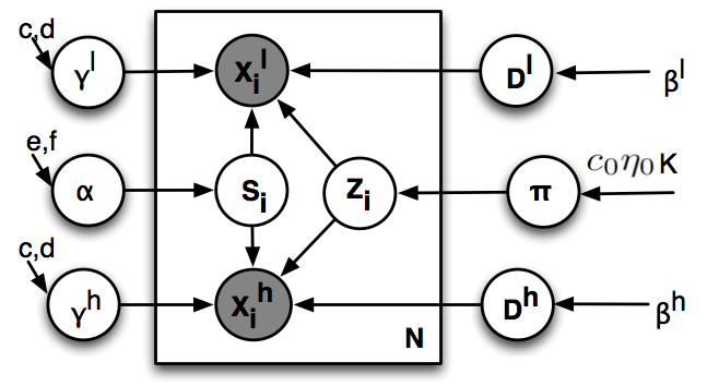
In the model, each small patch is generated from latent global dictionary elements—small images functioning as factor loadings—using local sparse weights and Gaussian noise. We will first explain how these latent variables are generated and then present how they are used to generate the observations.

We learn two dictionaries: one for high resolution images and one for low resolution images. In terms of notation, $\textbf{d}_{k}^{(l)}$ represents the LR dictionary element, and $\textbf{d}_{k}^{(h)}$ is the HR dictionary element. $P^{(l)}$ and $P^{(h)}$ represent the dimensionality of the low and high resolution dictionary elements, respectively. To model each dictionary element, we use a zero-mean Gaussian distribution,

$$\textbf{d}_{k}^{(l)}\mbox{ } \thicksim\mbox{ }\mathcal{N}(0,P^{(l)^{-1}}\textbf{I}_{P^{(l)}}) \textbf{d}_{k}^{(h)}\mbox{ } \thicksim\mbox{ }\mathcal{N}(0,P^{(h)^{-1}}\textbf{I}_{P^{(h)}}).$$

The matrix form of the dictionaries are $\textbf{D}^{(l)}$ and $\textbf{D}^{(h)}$ where $k$th columns of those matrices are $\textbf{d}_{k}^{(l)}$ and $\textbf{d}_{k}^{(h)}$, respectively.

Following [21], we assume that the sparse weights are shared by both resolution levels for combining dictionary elements to produce images. This is the key property of the model that allows us to frame super-resolution as inference. Sparse weights have two components: real valued weights $s_{ik}$ and binary valued assignments $z_{ik}$. To model the weights $s_{ik}$, we use a zero-mean Gaussian distribution with precision $\alpha$. $\textbf{z}_{i}$ is a binary vector that encodes which dictionary elements are activated for the corresponding observation. $p(\textbf{z})$ represents the prior of this variable and we will elaborate on this in next section. These are given as

$$s_{ik}\mbox{ } \thicksim\mbox{ }\mathcal{N}(0,1/\alpha) z_{ik}\mbox{ } \thicksim\mbox{ }p(z_{ik}).$$

We place Gamma priors on the precisions of the sparse weights and observation noise ($\alpha$ and $\gamma$). The two resolution levels share these variables as well,

$$\gamma\mbox{ } \thicksim\mbox{ }\mathrm{Gamma}(c,d), \alpha \sim\textrm{Gamma}(e,f).$$

Let $\textbf{x}_{i}^{(h)}$ and $\textbf{x}_{i}^{(l)}$ represents patches extracted from HR and LR images, respectively, as shown in Figure 1. Given the (global) dictionary elements and (local) sparse weights, the observations are modeled as

$$\boldsymbol{\epsilon}_{i}^{(l)} \thicksim\mathcal{N}(\textbf{0},\gamma^{-1}\textbf{I}_{P^{(l)}}) \boldsymbol{\epsilon}_{i}^{(h)} \thicksim\mathcal{N}(\textbf{0},\gamma^{-1}\textbf{I}_{P^{(h)}})$$

$$\textit{{x}}_{i}^{(l)} =\textbf{D}^{(l)}(\textbf{s}_{i}\odot\textbf{z}_{i})+\boldsymbol{\epsilon_{i}}^{(l)} \textit{{x}}_{i}^{(h)} =\textbf{D}^{(h)}(\textbf{s}_{i}\odot\textbf{z}_{i})+\boldsymbol{\epsilon_{i}}^{(h)}$$

where $\{(l),(h)\}$ represents LR and HR, respectively. Here, $N$ is the total number of patches, and $\odot$ represents the element-wise multiplication of two vectors. Figure 1 illustrates the graphical model.

To use this model in SR, we must be able to compute the posterior distributions of the hidden variables. In the training phase, we must compute the posterior distributions $p(\textbf{D}^{(h)},\textbf{D}^{(l)}|\{\textbf{x}_{i}^{(h)},\textbf{x}_{i}^{(l)}\})$ of the dictionaries, given a collection of HR/LR image pairs. In testing, we use their posterior expectation to reconstruct a held-out HR image from an LR image,

$$\mathbb{E}[\textbf{x}_{j}^{(h)}|\textbf{x}_{j}^{(l)},\{\textbf{x}_{i}^{(h)},\textbf{x}_{i}^{(l)}\}]\approx\hat{\textbf{D}}^{(h)}(\hat{\textbf{s}}_{j}\odot\hat{\textbf{z}}_{j})$$ (1)

where $\hat{\textbf{D}}^{(h)}$ is the mean of the posterior distribution $p(\textbf{D}^{(h)}|\{\textbf{x}_{i}^{(h)},\textbf{x}_{i}^{(l)}\})$ and $(\hat{\textbf{s}}_{j}\odot\hat{\textbf{z}}_{j})$ are the posterior expectation of the sparse weights from the LR image patches ($\textit{{x}}_{j}^{(l)}$) via posterior inference. (We discuss algorithms for posterior inference in Section III.)

II-A Beta-Bernoulli Process Prior (BP)

We now discuss the prior for the factor assignments $\textbf{z}_{i}$. We use a beta-Bernoulli process (BP) [22, 23, 24, 25, 26, 27, 28, 29], a prior on infinite binary matrices which is connected to the Indian buffet process (IBP). Each row encodes which dictionary elements are activated for the corresponding observation; columns with at least one active cell correspond to factors. The distinguishing characteristic of this prior is that the number of these factors is not specified a priori. Conditioned on the data, we examine the posterior distribution of the binary matrix to obtain a data-dependent distribution of how many components are needed.

The IBP metaphor gives the intuition. Consider a buffet of dishes at a restaurant. Suppose there are infinite number of dishes and we are trying to specify the infinite binary matrix indicating which customers (observations) choose which dishes (factors/dictionary elements). In the Indian buffet process (IBP), $N$ customers enter the restaurant sequentially. Each customer chooses dishes in a line from a buffet. The first customer starts from the beginning of the buffet and takes from each dish, stopping after Poisson($\tau$) number of dishes. The $i$th customer starts from the beginning as well, but decides to take from dishes in proportion to their popularity within the previous $i-1$ customers. This proportionality can be quantified as $\frac{m_{k}}{i}$ where $m_{k}$ is the number of previous customers who took this $k$th dish. After considering the dishes previously taken by other customers, the $i$th customer tries a Poisson($\frac{\tau}{i}$) number of new dishes. Which customers chose which dishes is recorded by the infinite binary matrix with $N$ rows (indicating the customers/observations) and infinite columns (indicating the dishes/factors/dictionary elements). One important (and surprising) property of this process is that the joint probability of final assignment is independent of the order of customers getting into the restaurant which is called exchangeability property of the prior [33].

The probabilistic construction is as follows. Each observation $i$ is drawn from a Bernoulli process (a sequence of independent identically distributed Bernoulli trials), $\textbf{x}_{i}\sim\mbox{BeP}(B)$ where $B$ is drawn from a beta process $B\sim\mbox{BP}(c_{0},B_{0})$. $B_{0}$ represents the base measure with $B_{0}={\cal N}(0,1/\beta\textbf{I})$. As $K\rightarrow\infty$, the $i$th observation is $\textbf{x}_{i}=\sum_{k=1}^{\infty}z_{ik}\delta_{d_{k}}$ where $z_{ik}$ denotes whether the dictionary element $\textbf{d}_{k}$ is used while representing the $i$th observation or not, and the sample from the beta process is given by $B=\sum_{k=1}^{\infty}\pi_{k}\delta_{d_{k}}$. Here, $\pi_{k}$ represents the usage probability of dictionary element $\textbf{d}_{k}$.

Figure 2: Graphical Model.

In inference, we use a finite beta-Bernoulli approximation [25]. The finite model truncates the number of dictionary elements to $K$ and is given by

$$\pi_{k}\sim\mathrm{Beta}(c_{0}\eta_{0},c_{0}(1-\eta_{0})),\mbox{ }z_{ik}\sim\textrm{Bernoulli}(\pi_{k})$$

where $c_{0}$ and $\eta_{0}$ are scalars and $\quad k\in 1,\ldots K$. As $K$ tends to infinity, the finite beta-Bernoulli approximation approaches the IBP/BP. If the truncation is large enough, data analyzed with this prior will exhibit fewer than $K$ components [23].

II-B Super-resolution via Posterior Distributions

Our algorithm has 2 stages: fitting the model on pairs of HR and LR images, and super-resolving new LR images to create HR versions.

Training: Coupled Dictionary Learning Stage. In training, we observe $\textbf{x}_{i}^{(h)}$ and $\textbf{x}_{i}^{(l)}$. All other random variables are latent. The key inference problem to be solved is the computation of the posterior distributions of the hidden variables. In the training phase, we must compute the posterior distributions $p(\textbf{D}^{(h)},\textbf{D}^{(l)}|\{\textbf{x}_{i}^{(h)},\textbf{x}_{i}^{(l)}\})$ of the dictionaries given a collection of HR/LR image pairs. We rewrite the coupled model in a form similar to the single scale model:

$$\textit{{x}}_{i}^{(c)}=\!\left(\!\begin{array}[]{c}\textit{{x}}_{i}^{(l)}\\ \textit{{x}}_{i}^{(h)}\end{array}\!\right)\!,\textbf{d}_{k}^{(c)}=\!\left(\!\begin{array}[]{c}\textbf{d}_{k}^{(l)}\\ \textbf{d}_{k}^{(h)}\end{array}\!\right)\!,\boldsymbol{\epsilon}_{i}^{(c)}=\!\left(\!\begin{array}[]{c}\boldsymbol{\epsilon}_{i}^{(l)}\\ \boldsymbol{\epsilon}_{i}^{(h)}\end{array}\!\right)\!$$ (8)

where the superscript $(c)$ corresponds to combination of $(l)$ and $(h)$. Writing the fully-observed model in this way reveals that we can train the dictionaries with similar methods as for the single-scale base model (Training amounts to approximating the posteriors of these values). The differences are that we use combined patches $\textit{{x}}_{i}^{(c)}$ and combined dictionaries $\textbf{d}_{k}^{(c)}$. This leads to shared sparse weights for the two resolution levels. (The details of how we compute the distribution $p(\textbf{D}^{(h)},\textbf{D}^{(l)}|\{\textbf{x}_{i}^{(h)},\textbf{x}_{i}^{(l)}\})$ are discussed in Section III.)

Super-resolving a Low Resolution Image. With fitted dictionaries in hand, we now show how to form HR images from LR images via posterior computation.

In this prediction setting, the HR image $\textbf{x}_{i}^{(h)}$ is unknown; the goal is to reconstruct it from the LR image patches $\textbf{x}_{i}^{(l)}$, the posterior estimates of the dictionaries $(\hat{\textbf{D}}^{(h)},\hat{\textbf{D}}^{(l)})$, and the precisions $\hat{\gamma},\hat{\alpha}$ of the noise and the sparse weights,

$$\textit{{x}}_{i}^{(c)}=\left(\begin{array}[]{c}\textit{{x}}_{i}^{(l)}\\ -\end{array}\right),\mbox{ }\textbf{d}_{k}^{(c)}=\left(\begin{array}[]{c}\textbf{d}_{k}^{(l)}\\ \textbf{d}_{k}^{(h)}\end{array}\right),\mbox{ }\boldsymbol{\epsilon}_{i}^{(c)}=\left(\begin{array}[]{c}\boldsymbol{\epsilon}_{i}^{(l)}\\ -\end{array}\right).$$

First we find estimates of the sparse factor scores, $(\hat{\textbf{s}}_{i}\odot\hat{\textbf{z}}_{i})$, by using the LR image patches $\textit{{x}}_{i}^{(l)}$ and posterior estimates of the dictionaries and precisions $\gamma$ and $\alpha$. The fitted value of $\alpha$ determines the strength of a “regularization term" that controls the sparsity of the factor scores.

More precisely, this prediction setting has 3 steps. The input is a set of held-out LR image patches $\textbf{x}_{i}^{(l)}$, the posterior estimates of the dictionaries $(\hat{\textbf{D}}^{(h)},\hat{\textbf{D}}^{(l)})$, and the precisions $\hat{\gamma},\hat{\alpha}$ of the noise and the sparse weights. The steps are as follows:

1. We find estimates of the sparse factor scores, $(\hat{\textbf{s}}_{i}\odot\hat{\textbf{z}}_{i})$, conditioned on the LR image patches $\textit{{x}}_{i}^{(l)}$ and estimates $(\hat{\textbf{D}}^{(h)},\hat{\textbf{D}}^{(l)}),\hat{\gamma},\hat{\alpha}$ from the training stage.

2. Eq. 1 determines the HR patches $\hat{\textbf{x}}_{i}^{(h)}\!$.

3. We replace each $\textbf{x}_{i}^{(l)}$ by its corresponding collocated $\hat{\textbf{x}}_{i}^{(h)}\!$; the whole HR image, $\hat{\textbf{X}}^{(h)}\!$, is the pixel-wise average of those overlapping reconstructions.

Post-processing: Following [21], we apply a post-processing step that, when down-sampled, the reconstructed HR image, $\hat{\textbf{X}}^{(h)}$, should match the given LR image $\textbf{X}^{(l)}$. Specifically, we solve the following optimization:

$$\hat{\textbf{X}}^{(h)*}=\underset{\textbf{X}}{\operatorname{argmin}}||f(\textbf{X})-\textbf{X}^{(l)}||_{2}^{2}+c||f(\textbf{X})-\hat{\textbf{X}}^{(h)}||_{2}^{2}$$

where $f()$ is a linear operator consisting of an anti-aliasing filter followed by down-sampling. This optimization problem is solved with gradient descent.

III Posterior Inference

In the proposed approach, all of the priors are in the conjugate exponential family. In a first implementation, we use Gibbs sampling. We iteratively sample from the conditional distribution of each hidden variable given the others and the observations. This defines a Markov chain whose stationary distribution is the posterior [34]. The corresponding sampling equations are analytic and provided in the appendix A-B (appendix is in the supplementary material).

The Gibbs sampler has difficulty with scaling to large data, because it must go through many iterations, each time visiting the entire data set before the sampler mixes. For this reason, both our Gibbs sampler and ScSR use $10^{5}$ patches sampled from $3\times 10^{6}$. We now develop here an alternative algorithm to Gibbs sampling for SR that scales to large and streaming data. Specifically, we develop an online variational inference algorithm.

Variational inference is a deterministic alternative to MCMC that replaces sampling with optimization. The idea is to posit a parameterized family of distribution over the hidden variables and then optimize the parameters to minimize the KL divergence to the posterior of interest [35]. Our algorithm iteratively tracks an approximate posterior distribution, which improves as more data are seen.

In typical applications, the variational objective is optimized with coordinate ascent, iteratively optimizing each parameter while holding the others fixed. However, in Bayesian settings, this suffers from the same problem as Gibbs sampling—the entire data set must be swept through multiple times in order to find a good approximate posterior. In the algorithm we present here, we replace coordinate ascent optimization with stochastic optimization—at each iteration, we subsample our data and then adjust the parameters according to a noisy estimate of the gradient. Because we only to subsample the data at each iteration, rather than analyze the whole data set, the resulting algorithm scales well to large data. This technique was pioneered in [36] and was recently exploited for online learning of topic models [37] and hierarchical Dirichlet processes [38].

We first develop the coordinate ascent algorithm for the coupled model. Then we derive the online variational inference algorithm, which can more easily handle large data sets.

III-A Variational Inference for the Coupled model

We use the coupling perspective in Section II-B to derive the batch variational Bayes (VB) algorithm. The single-scale base model is the BPFA model of [26], which gives a mean-field variational inference algorithm. The batch VB algorithm derived here is the coupled version of that.

We first define a parametrized family of distributions over the hidden variables. Let $\textbf{Q}=\{\boldsymbol{\pi},\textbf{Z, S, D},\gamma,\alpha\}$ denote the hidden variables for all $i,k$. We write coupled data as in Equation 8; in the new set-up the variables to be learned become $\textbf{Q}=\{\boldsymbol{\pi},\textbf{Z, S},\textbf{D}^{(c)},\gamma,\alpha\}$. We use a fully factorized variational distribution,

$$q(\textbf{Q})=q_{\tau}(\boldsymbol{\pi})q_{\phi}(\textbf{D}^{(c)})q_{\nu}(\textbf{Z})q_{\theta}(\textbf{S})q_{\lambda}(\boldsymbol{\gamma})q_{\epsilon}(\boldsymbol{\alpha}).$$

Each component of this distribution is governed by a free variational parameter,

$$q_{\tau_{k}}(\pi_{k}) =\mathrm{Beta}(\tau_{k1},\tau_{k2}) q_{\nu_{ik}}(z_{ik}) =\mathrm{Bernoulli}(\nu_{ik})$$

$$q_{\phi_{kj}}(d_{kj}) =\mathcal{N}(\phi_{kj},\Phi_{kj}) q_{\lambda}(\gamma) =\mathrm{Gamma}(\lambda_{1},\lambda_{2})$$

$$q_{\theta_{ik}}(s_{ik}) =\mathcal{N}(\theta_{ik},\Theta_{ik}) q_{\epsilon}(\alpha) =\mathrm{Gamma}(\epsilon_{1},\epsilon_{2})$$

We optimize these parameters with respect to a bound on the marginal probability of the observations. This bound is equivalent, up to a constant, to the negative KL divergence between $q$ and the true posterior. Thus maximizing the bound is equivalent to minimizing KL divergence to the true posterior. Let $\boldsymbol{\Xi}=\{c_{0},\eta_{0},c,d,e,f\}$ be the hyper-parameters. The variational lower bound is

$$\log(p(\textbf{X}^{(c)}|\boldsymbol{\Xi}))\geq H(q)+\sum\nolimits_{k=1}^{K}\Big{\{}\mathbb{E}_{\textbf{q}}[\log p(\pi_{k}|c_{0},\eta_{0},K)]$$

$$+\sum\nolimits_{i=1}^{N}\mathbb{E}_{\textbf{q}}[\log p(z_{ik}|\boldsymbol{\pi})]+\sum\nolimits_{j=1}^{J}\mathbb{E}_{\textbf{q}}[\log\big{(}p(d_{kj}|\beta_{kj})\big{)}]$$

$$+\sum\nolimits_{i=1}^{N}\mathbb{E}_{\textbf{q}}[\log\big{(}p(s_{ik}|\alpha)p(\alpha|e,f)\big{)}]\Big{\}}$$ (9)

$$+\sum\nolimits_{i=1}^{N}\Big{\{}\mathbb{E}_{\textbf{q}}[\log p(\textbf{x}_{i}^{(c)}|\textbf{Z,S,}\textbf{D}^{(c)}\gamma)]+\mathbb{E}_{\textbf{q}}[\log p(\gamma|c,d)]\Big{\}},$$

where $\textrm{H}(q)$ is the entropy of the variational distribution and dimensionality of the dictionary elements $J$ is twice as big as the single-scale model. We denote this function ${\cal L}(q)$.

Holding the other parameters fixed, we can optimize each variational parameter exactly; this gives an algorithm that goes uphill in ${\cal L}(q)$ [39]. (Further, this will provide the algorithmic components needed for the online algorithm of Section III-B.)

Update equations for each free parameter optimizing this bound are given below. In all equations, $\textbf{I}_{P}$ represents $P\times P$ identity matrix, and $\tilde{\textbf{x}}_{i(-k)}^{(c)}$ represents the reconstruction error using all but the $k$th dictionary element, that is

$$\tilde{\textbf{x}}_{i(-k)}^{(c)}=\textbf{x}_{i}^{(c)}-\textbf{D}^{(c)}(\textbf{s}_{i}\odot\textbf{z}_{i})+\textbf{d}_{k}^{(c)}(s_{ik}\odot z_{ik}).$$

The expectation based on the variational distribution is then given by

$$\mathbb{E}_{q}[\tilde{\textbf{x}}_{i(-k)}^{(c)}]=\textbf{x}_{i}^{(c)}+\boldsymbol{\phi}_{k}^{(c)}(\theta_{ik}\nu_{ik})-\sum_{k=1}^{K}\boldsymbol{\phi}_{k}^{(c)}(\theta_{ik}\nu_{ik}).$$

Update for the binary factor assignment $z_{ik}$: The variational parameter for factor assignment $z_{ik}$ is $\nu_{ik}$. We first consider two values of the variational distribution for two values (0,1) of $z_{ik}$,

$$q(z_{ik}=1)\mbox{ } \propto\mbox{ }\exp(\mathbb{E}_{q}[\ln(\pi_{k})])\mbox{exp}\Big{(}-\frac{\frac{\lambda_{1}}{\lambda_{2}}\big{(}(\theta_{ik}^{2}+\Theta_{ik})(\boldsymbol{\phi}_{k}^{(c)^{T}}\boldsymbol{\phi}_{k}^{(c)}+\sum_{j}\Phi_{kj})-2\theta_{ik}\boldsymbol{\phi}_{k}^{(c)^{T}}\mathbb{E}_{q}[\tilde{\textbf{x}}_{i(-k)}^{(c)}]\big{)}}{2}\Big{)}$$

$$q(z_{ik}=0)\mbox{ } \propto\mbox{ }\exp(\mathbb{E}_{q}[ln(1-\pi_{k})]),\mbox{ }\mbox{where}$$

$$\mathbb{E}_{q}[\ln(\pi_{k})]\mbox{ } =\mbox{ }\psi\big{(}c_{0}\eta_{0}+\sum_{i}\nu_{ik}\big{)}-\psi(c_{0}+N)$$

$$\mathbb{E}_{q}[\ln(1-\pi_{k})]\mbox{ } =\mbox{ }\psi\big{(}c_{0}(1-\eta_{0})-\sum_{i}\nu_{ik}+N\big{)}-\psi(c_{0}+N)$$

Then the update equation for the variational parameter $\nu_{ik}$ is given as

$$\nu_{ik}\mbox{ } =\mbox{ }\frac{q(z_{ik}=1|-)}{q(z_{ik}=1|-)+q(z_{ik}=01|-)}$$

Update for the shared sparse weight $s_{ik}$: The variational distribution for the sparse weight $s_{ik}$ is Gaussian parametrized with mean $\theta_{ik}$ and variance $\Theta_{ik}$. Coordinate ascent update equation for these free variational parameters are

$$\Theta_{ik}\mbox{ } =\mbox{ }\Big{(}\frac{\epsilon_{1}}{\epsilon_{2}}+\frac{\lambda_{1}}{\lambda_{2}}\nu_{ik}(\boldsymbol{\phi}_{k}^{(c)^{T}}\boldsymbol{\phi}_{k}^{(c)}+\sum_{j}\Phi_{kj})\Big{)}^{-1}$$

$$\theta_{ik}\mbox{ } =\mbox{ }\frac{\lambda_{1}}{\lambda_{2}}\Theta_{ik}\nu_{ik}\boldsymbol{\phi}_{k}^{(c)^{T}}\mathbb{E}_{q}[\tilde{\textbf{x}}_{i(-k)}^{(c)}].$$

Update for the $k$th coupled dictionary element $\textbf{d}_{k}^{(c)}$: The variational distribution for the couple dictionary element $\textbf{d}_{k}^{(c)}$ is Gaussian parametrized with mean $\boldsymbol{\phi}_{k}^{(c)}$ and variance $\boldsymbol{\Phi}_{k}^{(c)}$. Coordinate ascent update equation for these free variational parameters are

$$\boldsymbol{\Phi}_{k}^{(c)}\mbox{ } =\mbox{ }\Big{(}2P\textbf{I}_{2P}+\frac{\lambda_{1}}{\lambda_{2}}\sum_{i=1}^{N}(\theta_{ik}^{2}+\Theta_{ik})\nu_{ik}^{2}\Big{)}^{-1}$$

$$\boldsymbol{\phi}_{k}^{(c)}\mbox{ } =\mbox{ }\frac{\lambda_{1}}{\lambda_{2}}\boldsymbol{\Phi}_{k}^{(c)}\sum_{i=1}^{N}\theta_{ik}\nu_{ik}\mathbb{E}_{q}[\tilde{\textbf{x}}_{i(-k)}^{(c)}].$$

The updates for high resolution (h) and low resolution (l) components can be given separately as

$$\boldsymbol{\Phi}_{k}^{(h)}\mbox{ } =\mbox{ }\Big{(}2P\textbf{I}_{P}+\frac{\lambda_{1}}{\lambda_{2}}\sum_{i=1}^{N}(\theta_{ik}^{2}+\Theta_{ik})\nu_{ik}^{2}\Big{)}^{-1} \boldsymbol{\Phi}_{k}^{(l)}\mbox{ } =\mbox{ }\Big{(}2P\textbf{I}_{P}+\frac{\lambda_{1}}{\lambda_{2}}\sum_{i=1}^{N}(\theta_{ik}^{2}+\Theta_{ik})\nu_{ik}^{2}\Big{)}^{-1}$$

$$\boldsymbol{\phi}_{k}^{(h)}\mbox{ } =\mbox{ }\frac{\lambda_{1}}{\lambda_{2}}\boldsymbol{\Phi}_{k}^{(h)}\sum_{i=1}^{N}\theta_{ik}\nu_{ik}\tilde{\textbf{x}}_{i(-k)}^{(h)} \boldsymbol{\phi}_{k}^{(l)}\mbox{ } =\mbox{ }\frac{\lambda_{1}}{\lambda_{2}}\boldsymbol{\Phi}_{k}^{(l)}\sum_{i=1}^{N}\theta_{ik}\nu_{ik}\tilde{\textbf{x}}_{i(-k)}^{(l)}.$$

Update for the dictionary usage probabilities $\pi_{k}$: The variational distribution for the dictionary usage probabilities $\pi_{k}$ is a beta distribution parametrized with the shape parameters ($\tau_{k1},\tau_{k2}$). Coordinate ascent update equation for these free variational parameters are

$$\tau_{k1}\mbox{ } =\mbox{ }c_{0}\eta_{0}+\sum_{i=1}^{N}\nu_{ik}$$

$$\tau_{k2}\mbox{ } =\mbox{ }\mbox{ }N-\sum_{i=1}^{N}\nu_{ik}+c_{0}(1-\eta_{0}).$$

Update for the precision $\gamma$: The variational distribution for the precision $\gamma$ of the observation noise $\boldsymbol{\epsilon}_{i}$ is a gamma distribution parametrized with ($\lambda_{1},\lambda_{2}$). Coordinate ascent update equation for these free variational parameters are

$$\lambda_{1}\mbox{ } =\mbox{ }c+NP$$

$$\lambda_{2}\mbox{ } =\mbox{ }d+\frac{1}{2}\sum_{i=1}^{N}\Big{\{}||\textbf{x}_{i}^{(c)}-\sum_{k=1}^{K}\boldsymbol{\phi}_{k}^{(c)}(\theta_{ik}\nu_{ik})||_{2}^{2}+\sum_{k=1}^{K}\nu_{ik}(\theta_{ik}^{2}+\Theta_{ik})(\boldsymbol{\phi}_{k}^{(c)^{T}}\boldsymbol{\phi}_{k}^{(c)}+\sum_{j}\Phi_{kj})$$

$$-\mbox{ }\sum_{k=1}^{K}\nu_{ik}\boldsymbol{\phi}_{k}^{(c)^{T}}\boldsymbol{\phi}_{k}^{(c)}\theta_{ik}^{2}\Big{\}}.$$

Update for the precision $\alpha$: The variational distribution for the precision $\alpha$ of the sparse weights $s_{ik}$ is a gamma distribution parametrized with ($\epsilon_{1},\epsilon_{2}$). Coordinate ascent update equation for these free variational parameters are

$$\epsilon_{1}\mbox{ } =\mbox{ }e+\frac{1}{2}NK$$

$$\epsilon_{2}\mbox{ } =\mbox{ }f+\frac{1}{2}\sum_{i=1}^{N}\sum_{k=1}^{K}(\theta_{ik}^{2}+\Theta_{ik}^{2}).$$

Algorithm 1 Batch VB

  Sample $N$ observations from the data. Initialize $\boldsymbol{\tau},\boldsymbol{\nu},\boldsymbol{\phi},\boldsymbol{\Phi},\boldsymbol{\theta},\boldsymbol{\Theta},\boldsymbol{\lambda},\boldsymbol{\epsilon}$ using Gibbs sampler.

  for $t=1$ to $T$ do

     Init. local variables $\nu_{n_{k}},\boldsymbol{\theta}_{n_{k}},\boldsymbol{\Theta}_{n_{k}}$ using Gibbs sampler.

     while relative improvement in $\ell$ is large  do

        for $k=1$ to $K$ do

           for $n=1$ to $N$ do

              update $\nu_{nk},\boldsymbol{\theta}_{nk},\boldsymbol{\Theta}_{nk}$ by using batch VB updates.

           compute $\Phi_{k},\boldsymbol{\phi}_{k},\boldsymbol{\tau}_{k},\boldsymbol{\lambda},\boldsymbol{\epsilon}$ by batch VB updates.

III-B Online Variational Inference

We now develop online variational inference. We divide the variational parameters into global variables and local variables. Global variables depend on all of the images. These are the dictionary probabilities $\boldsymbol{\pi}_{k}$, dictionary elements $\textbf{d}_{k}$, precisions $\boldsymbol{\alpha}$ and $\gamma$. Local variables are the ones drawn for each image. These are the weights $\textbf{s}_{i}$, binary variables $\textbf{z}_{i}$. The algorithm iterates between optimizing the local variables using local (per-image) coordinate ascent, and optimizing the global variables. This same structure is found in many Bayesian nonparametric models  [23, 40].

The basic idea is to optimize Equation 9 via stochastic optimization [41]. This means we repeatedly follow noisy estimates of the gradient with decreasing step sizes $\rho_{t}$. If the step sizes satisfy $\textstyle\sum_{t}\rho_{t}=\infty$ and $\textstyle\sum_{t}\rho^{2}_{t}<\infty$ then we will converge to the optimum of the objective. (In variational inference, we will converge to a local optimum.)

Algorithm 2 Online VB with mini-batches

  Define $\rho_{t}=(r+t)^{-\kappa}$, Initialize $\boldsymbol{\tau},\boldsymbol{\nu},\boldsymbol{\phi},\boldsymbol{\Phi},\boldsymbol{\theta},\boldsymbol{\Theta},\boldsymbol{\lambda},\boldsymbol{\epsilon}$ using Gibbs sampler.

  for $t=1$ to $\frac{N}{N_{S}}$ do

     Sample $N_{S}$ new observations from the data. Initialize local variables $\nu_{n_{k}},\boldsymbol{\theta}_{n_{k}},\boldsymbol{\Theta}_{n_{k}}$ using Gibbs sampler.

     while relative improvement in $\ell$ is large  do

        for $k=1$ to $K$ do

           for $n_{t}=(t-1)\times N_{S}+1$ to $t\times N_{S}$ do

              update $\nu_{n_{t}k},\boldsymbol{\theta}_{n_{t}k},\boldsymbol{\Theta}_{n_{t}k}$ by using batch VB updates.

           compute $\tilde{\Phi}_{k},\tilde{\boldsymbol{\phi}}_{k},\tilde{\boldsymbol{\tau}}_{k},\tilde{\boldsymbol{\lambda}},\tilde{\boldsymbol{\epsilon}}$ by batch VB updates as if there are $N/N_{S}$ copies of the images.

     for $k=1$ to $K$ do

        update $\Phi_{k},\boldsymbol{\phi}_{k},\boldsymbol{\tau}_{k},\boldsymbol{\lambda},\boldsymbol{\epsilon}$ by Equation 12

The noisy estimates of the gradient are obtained from subsampled data. We write the objective $\mathcal{L}$ as a sum over data points. Defining the distribution $g(n)$ which uniformly samples from the data, we can then write $\mathcal{L}$ as an expectation under this distribution,

$$\mathcal{L} =\sum\nolimits_{n=1}^{N}\ell(\boldsymbol{\tau},\boldsymbol{\nu}_{n},\boldsymbol{\phi},\boldsymbol{\theta}_{n},\boldsymbol{\lambda}_{n},\boldsymbol{\epsilon}_{n},\textbf{X}_{n}).$$ (10)

$$=N\mathbb{E}_{g}[\ell(\boldsymbol{\tau},\boldsymbol{\nu}_{n},\boldsymbol{\phi},\boldsymbol{\theta}_{n},\boldsymbol{\Theta}_{n},\boldsymbol{\lambda}_{n},\boldsymbol{\epsilon}_{n},\textbf{X}_{n})]$$ (11)

The gradient of the objective can be written as a similar expectation. Thus, sampling data at random and computing the gradient of $\ell_{n}$ gives a noisy estimate of the gradient.

Figure 3: Dictionary trained in batch mode on lluminance channel with SR ratio = 2. (Left) HR Dictionary, (Right) LR Dictionary, Every square represents a dictionary element and the HR-LR pairs are co-located. HR dictionary consists of sharper edges.

There are two further simplifications. First, when we subsample the data we optimize the local variational parameters fully and compute the gradient of $\ell_{n}$ with respect to only the global variational parameters. Second, we use the natural gradient [42] rather than the gradient. In mean field variational inference, this simplifies the gradient step as follows. Suppose we have sampled an image $n$ and fitted its local variational parameters given the current settings of the global variational parameters. Let $\tilde{\boldsymbol{\tau}},\tilde{\boldsymbol{\phi}},\tilde{\boldsymbol{\Phi}},\tilde{\boldsymbol{\lambda}},\tilde{\boldsymbol{\epsilon}}$ be the global variational updates from Section III-A as though we observed $N$ copies of that image. (Note that these depend on its local variational parameters.) Following a noisy estimate of the natural gradient of ${\cal L}$ is equivalent to taking a weighted average of the current and the newly fitted global parameters, e.g.

$$\boldsymbol{\phi}=(1-\rho_{t})\boldsymbol{\phi}+\rho_{t}\tilde{\boldsymbol{\phi}}.$$ (12)

It follows that there is no additional computational cost to optimizing the global variational parameters with stochastic optimization versus coordinate ascent.

In our implementation, we decrease the step-size $\rho_{t}$ by $\rho_{t}=(\rho_{0}+t)^{-\kappa}$. The learning rate parameter $\rho_{0}$ down-weights early iterations; the parameter $\kappa$ controls the speed of forgetting previous values of the global variables.

The full online VB algorithm is listed in Algorithm 2. (Note that we sample the data in mini-batches, rather than one at a time. When the mini-batch size is equal to one data point, we recover the algorithm as described above.)

III-C Initialization with MCMC.

We initialize both the batch and online VB with a few iterations (e.g. 5 or 10) of MCMC. This is useful for two reasons: (1) It provides a good initialization and thus faster convergence, (2) Noisy random-walks of MCMC help VB avoid low-quality local optima: at the beginning of each e-step, MCMC initializes $\textbf{s}_{i}$ and $\textbf{z}_{i}$ by sampling from their approximate posterior distribution, given the most recent global variables. These samples are noisy estimates of the sparse weights near their posterior means. For instance, when the factor assignment $z_{ik}$ equals $0$, the MCMC draws the sparse weight $s_{ik}$ from the prior $\mathcal{N}(0,1/\alpha)$ whereas in VB it would be exactly 0. Providing the freedom to “jiggle" gives the algorithm the opportunity, similar to simulated annealing, to jump away from one local optimum to reach a better optimum.

IV Experiments

We use three data sets. To train, we use the set of 68 images collected from the web by [21]. We test on the Berkeley natural image data set (20 100$\times$100 images) and a benchmark set of images (11 images of various size) used by the community to evaluate SR algorithms. These data sets provide us with a rich set of HR-LR pairs.

TABLE I: Test Results with SR ratio = 2. PSNR for the illuminance channel is presented (the higher the better). BP: Proposed algorithm trained via Gibbs sampler, O-BP Proposed algorithm trained via Online VB, seeing more data, ScSR: Super-Resolution via Sparse Representation [21], NNI: Nearest neighbor interpolation, SME: Sparse Mixing Estimation [43].

PSNR	Bic.	NNI	Bil.	SME	ScSR256	ScSR512	BP	OBP
Baboon	23.63	23.12	23.05	23.10	24.33	24.36	24.27	24.39
Barbara	25.35	25.10	24.92	24.42	25.88	25.89	25.98	25.99
Boat	29.95	28.39	28.94	29.72	31.23	31.29	31.17	31.31
Camera	30.32	35.20	28.94	26.33	30.68	30.46	31.51	30.94
House	32.79	30.34	31.61	33.28	34.26	34.31	34.08	34.27
Peppers	31.99	29.88	31.18	33.06	33.05	33.06	32.45	33.08
Parthen.	28.12	27.28	27.42	27.28	29.05	29.10	28.96	29.06
Girl	34.76	33.44	33.98	33.98	35.57	35.58	35.62	35.66
Flower	40.04	37.96	38.94	39.72	41.06	41.11	41.26	41.33
Lena	32.83	31.00	31.72	33.57	34.47	34.54	34.56	34.68
Raccoon	30.95	29.82	29.95	31.73	32.39	32.43	32.43	32.62

Throughout this work, unless otherwise mentioned we use the same parameters (without any tuning): we set the SR ratio to 2 or 4 and the patch size to $8\times 8$. The hyper-parameters are $c=d=e=f=10^{-6}$ and $c_{0}=2,\eta_{0}=0.5$, these are standard uninformative priors used in e.g. [28]. The truncation level $K$ in BP is set to 512. Most images use fewer factors, e.g. Baboon uses 487, House 438 and Barbara 471 factors. We apply all algorithms only to the illuminance channel and use Bicubic interpolation for the color layers (Cb, Cr) for all compared methods.

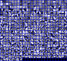
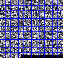
We study our methods with two kinds of posterior inference—Gibbs sampling (BP) and online variational inference (O-BP), which scales to larger data sets. To compare, we study both interpolation and example-based algorithms. Bicubic interpolation is the gold standard in the SR literature. We also study nearest neighbor interpolation, bilinear interpolation and sparse mixing estimation (SME) [43]. To compare with an example-based method, we use super-resolution via sparse representation (ScSR, [21]). Both BP’s and ScSR’s dictionary learning stages use $10^{5}$ patches sampled from the training data, however O-BP uses the whole set in online fashion. The HR and LR dictionaries trained by our approach are shown in Figure 3. The HR dictionary consists of sharper edges.

TABLE II: Test Results with SR ratio = 2. PSNR for the illuminance channel is presented (the higher the better). BP: Proposed algorithm trained via Gibbs sampler, O-BP Proposed algorithm trained via Online VB, seeing more data, ScSR: Super-Resolution via Sparse Representation [21], NNI: Nearest neighbor interpolation.

PSNR	Bic.	NNI	Bilin.	ScSR256	ScSR512	BP	O-BP
N1	29.74	27.44	28.39	31.52	31.55	31.52	31.56
N2	29.52	27.71	28.27	31.16	31.20	31.17	31.20
N3	22.97	21.95	22.12	23.94	24.00	23.80	23.94
N4	21.63	20.98	20.90	22.59	22.66	22.38	22.41
N5	24.85	23.85	24.01	26.01	26.06	25.77	25.90
N6	25.34	24.61	24.70	26.20	26.26	26.08	26.07
N7	26.66	25.43	25.73	27.92	27.92	27.77	27.97
N8	26.08	24.71	25.23	27.27	27.43	27.01	27.26
N9	26.02	25.29	25.42	26.82	26.89	26.58	26.73
N10	24.79	24.07	23.92	26.23	26.25	25.91	26.16
N11	26.86	25.22	25.97	28.06	28.04	27.99	28.16
N12	28.16	26.65	27.07	29.63	29.66	29.78	29.86
N13	25.15	24.18	24.22	26.40	26.36	26.31	26.33
N14	26.82	25.98	25.92	27.99	28.01	27.86	27.94
N15	25.78	24.64	24.81	27.00	27.04	26.90	27.06
N16	27.28	25.85	26.16	28.88	29.01	28.83	28.96
N17	27.79	26.33	26.81	29.21	29.24	29.02	29.16
N18	29.13	27.75	28.18	30.38	30.41	30.25	30.43
N19	24.57	23.19	23.50	26.07	26.10	25.92	26.02
N20	22.00	21.13	21.05	23.26	23.28	23.26	23.29

As a quantitative measure of performance we compute the signal to noise ratio (PSNR), a measure that is widely used in image recovery applications. We present the PSNR results for benchmark images in Table I and natural images in Table II. These PSNR based results can be summarized as: (1) The online learning algorithm and ScSR performs similarly, (2) They both slightly perform better than the Gibbs sampler. (3) All of the example based algorithms perform better than the interpolation based techniques.

IV-A Evaluation and Crowdsourcing via Mechanical Turk

Though signal to noise ratio (PSNR), is a widely used metric in image recovery applications, this is not enough to measure human judgement. For this purpose, we also performed human evaluation experiments on Amazon Mechanical Turk (MTurk, http://www.mturk.com).

Figure 4: Human Evaluation via Mechanical Turk. (Top) Average win rate in one-to-one comparisons. (Bottom) Win rates for each one-to-one comparison. Each number represents the winning rate of the method in the column, e.g., $0.57$ for BP vs ScSR (BP is on the column and ScSR on the row) means that on average, 0.57 of the times Turkers voted in favor of BP.

The Amazon Mechanical Turk (MTurk) is a web interface for deploying small tasks to people, called Turkers. Typically an MTurk experiment works as follows: the requesters, people organizing the experiments and paying Turkers, prepare tasks called HITs (Human Intelligence Tasks). Each HIT might be a comparison of images, labeling of text etc. Once the HITs are completed, requesters can approve or reject the HITs based on their reliability measures (for instance trivial solution HITs, as we explain next, and the time spend on each HIT are frequently used measures for reliability). Approved results are acquired to be used in the analysis.

(a) High

(b) Low

(c) Bicubic

(d) NNI

(e) Bilinear

(f) ScSR

(g) BP

(h) O-BP

Figure 5: Reconstruction of Natural Image 3. BP: Algorithm presented in this work trained via Gibbs sampler, O-BP Algorithm presented in this work trained via Online VB, ScSR: Super-Resolution via Sparse Representation. Example based approaches are superior to interpolation techniques, ScSR and our approach perform similarly.

While preparing HITs, we used the natural image data. We asked Turkers to visually assess and select the better of two HR reconstructions of each image. We considered all ordered combinations of the algorithms, each equally likely, e.g., BP vs ScSR, BP vs Bicubic etc. We initially collected $42,807$ decisions from 208 unique Turkers. For quality control we gave test pairs in which a ground truth HR image was used, i.e., a comparison of an algorithmic reconstruction vs a true HR image. All of the judgments of the Turkers who failed to pass this test (Turkers who selected the algorithmic reconstruction instead of true HR) were removed. This reduced the data to $20,469$ decisions from 161 unique reliable Turkers.

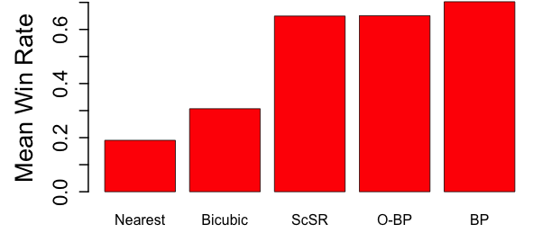
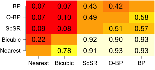
The results of the human evaluation are in Figure 4. In the bottom table, win rates for each one-to-one comparisons are provided. Each number represents the winning rate of the method in the column. For instance, $0.93$ for O-BP vs Nearest (O-BP is on the column and Nearest on the row) means that out of 100 binary comparisons of O-BP and Nearest, 93 of the times Turkers voted in favor of O-BP. In general, we observe that example-based methods perform significantly better than interpolation-based methods. Within the example-based approaches, the models are similar. However, our approach does not use the first and second-order derivative filters for the LR patches used by ScSR as features, yet we perform similarly; moreover we do not need to set the noise precision and the number of dictionary elements, both required parameters of ScSR (We used the parameters provided by [21] in ScSR.).

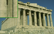
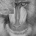
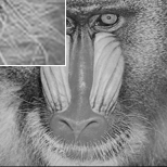
In the PSNR results, ScSR and O-BP seem to perform similarly and both slightly better than BP. However, in the human evaluation we observed that BP reconstructions are found to be better. (Based on 95% confidence intervals, both the BP vs O-BP and BP vs ScSR results are statistically significant. The O-BP vs ScSR difference is statistically insignificant.) This shows that PSNR is not necessarily consistent with the human assessment of images [45]. Sample visual results are shown in Figures 5, 6 and 7. (The remaining results are in the appendix E and F.)

(a) High

(b) Low

(c) Bicubic

(d) NNI

(e) Bilinear

(f) SME

(g) ScSR

(h) BP

(i) O-BP

Figure 6: Reconstruction of Parthenon Image. BP: Algorithm presented in this work trained via Gibbs sampler, O-BP Algorithm presented in this work trained via Online VB, ScSR: Super-Resolution via Sparse Representation. SME: Sparse Mixing Estimation [43]

(a) High

(b) Low

(c) Bicubic

(d) NNI

(e) Bilinear

(f) SME

(g) ScSR

(h) BP

(i) O-BP

Figure 7: Reconstruction of Baboon Image. BP: Algorithm presented in this work trained via Gibbs sampler, O-BP Algorithm presented in this work trained via Online VB, ScSR: Super-Resolution via Sparse Representation. SME: Sparse Mixing Estimation [43].

IV-B Nonparametric property of the model.

In this section, we demonstrate the importance of a Bayesian nonparametric method for image super-resolution. As we mentioned in Section II-A, we use a beta-Bernoulli process (BP) for the factor assignments $\textbf{z}_{i}$ that encodes which dictionary elements are activated for the corresponding observation. In the binary matrix (whose rows are the factor assignment $\textbf{z}_{i}$’s), the columns with at least one active cell correspond to factors that are used.

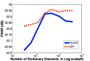
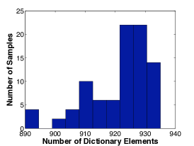
The distinguishing characteristic of this prior is that the number of the factors to be learned is not specified a priori. Conditioned on the data, we examine the posterior distribution of the binary matrix to obtain a data-dependent distribution of how many components are needed. For the parametric ScSR, the number of dictionary elements must be set a priori. This is illustrated by the following experiment. For both model, we train on $10^{4}$ patches, for different values of $K$ (starting from scratch each time); for ScSR, $K$ is the target number (which needs to be set before starting the algorithm), while for our approach, $K$ functions as an upper bound on the number of dictionary elements (which should not be too low). Figure 8 shows that, unlike ScSR, our approach is less sensitive to the value of $K$ if it is sufficiently large. The Barbara image uses 700, 801 and 816 factors in our approach for $K$ equals to $1024,2048$ and $4096$ respectively.

Figure 8: Learning the number of dictionary elements from the data. (Left) PSNR of the reconstruction of the Barbara image by nonparametric BP and parametric ScSR with different number of dictionary elements. (Right) Histogram of the number of dictionary elements for BP when $K=1024$ over 100 samples.

Figure 9: Held-out prediction performances of Online Learning with different mini-batch sizes. Online-VB run on the whole data set is compared with the Batch-VB run on a subset of the data. The online algorithms converge much faster than the batch algorithm does.

IV-C Online learning, Computational Time and Scaling

In this section, we compare the scale properties of the algorithms presented in this paper. In online learning, instead of subsampling the patches during the dictionary learning stage, we use the full data set and process the data segment by segment (so called "mini-batches"). We use the training data set of Section IV. The learning parameters are set to $\kappa=0.501$ and $\rho_{0}=3$.

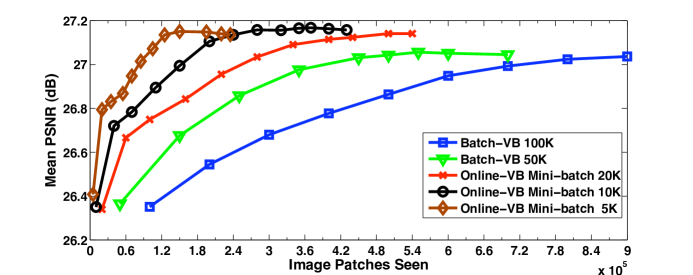
Figure 9 shows the evolution of the mean PSNR on the held-out natural image data set by the online and the batch algorithms as a function of the number of image patches seen (visualizations of the learned dictionaries are provided in appendix D). The number of patches seen represents the computational time since both algorithms’ time complexity is linear with number of observations. For online VB, the number of patches seen represents the total number of data seen after each iteration. For batch VB, this represents cumulative sum of the number of same data seen after each variational-EM iteration. Even before the second iteration of the batch VB (100K) is completed, online VB with 5K mini-batch converges – reaches to a local optima better than batch VB. This means that the online algorithm finds dictionaries at least as good as those found by the batch VB in only a fraction of the time. As also shown in Table I, it finds high quality dictionaries. This may be because stochastic gradient is robust to local optima [46].

For dictionary training, the convergence time for online VB with 5K mini-batch size is 16 hours. In Gibbs sampling, we throw away the first 1500 samples for the burn-in period and later collect 1500 samples to approximate the posterior distributions. This takes approximately 50 hours on the same machine with an unoptimized Matlab implementation on $10^{5}$ number of patches. Running Gibbs sampling same amount of time with online VB, i.e. collecting less number of samples such as 500, reduces held-out PSNR between $0.2$ dB to $0.5$ dB, depending on the image. This is consistent with the findings in [28].

V Discussion

We developed a new model for super-resolution based on Bayesian nonparametric factor analysis, and new algorithms based on Gibbs sampling and online variational inference. With online training, our algorithm scales to very large data sets. We evaluated our method against a leading sparse coding technique [21] and other state of the art methods. We evaluated both with traditional PSNR and by devising a large scale human evaluation. This is a new real-world application that can utilize online variational methods.

The choice of the inference algorithm depends on the usage case. Our results suggest that with more computation time Gibbs sampling performs slightly better (based on human evaluation). If speed is important, our online algorithms can be used without much loss.

Regarding the evaluation metric, the standard in image analysis has been signal-to-noise ratio (PSNR). However, its practical relevance has been questioned [45]. The human eye is sensitive to details which are not always captured in this metric, and that is why we ran a human evaluation. Our experiments show that the signal-to-noise ratio is not necessarily consistent with human judgement.

As future work, our approach can be used as a building block in other, more complicated, probabilistic models. For example, our approach could be developed into a time series to perform super-resolution on video or a hierarchical model can be built that fully generates the whole image instead of patch based approach.

TABLE III: Test Set Results with SR ratio = 4. PSNR for the illuminance channel (higher the better). BP: Algorithm presented in this paper with Beta Process (BP) Prior trained with Gibbs Sampler, ScSR: Super-Resolution via Sparse Representation, NNI: Nearest neighbor interpolation.

PSNR	Bicubic	NNI	Bilinear	ScSR	BP
N1	24.58	22.80	23.77	25.36	25.15
N2	24.81	23.54	24.18	25.51	25.28
N3	18.97	18.43	18.60	19.39	19.38
N4	18.11	17.78	17.83	18.50	18.37
N5	21.17	20.60	20.78	21.72	21.54
N6	22.12	21.68	21.84	22.43	22.41
N7	22.62	21.62	22.20	23.13	23.12
N8	22.00	20.82	21.53	22.59	22.47
N9	22.90	22.27	22.59	23.10	23.16
N10	21.39	21.04	21.22	21.53	21.55
N11	22.82	21.28	22.22	23.51	23.41
N12	24.09	23.10	23.53	24.74	24.66
N13	21.13	20.42	20.77	21.42	21.45
N14	23.06	22.50	22.72	23.31	23.33
N15	21.79	21.15	21.45	22.11	22.16
N16	22.52	21.58	22.05	23.00	22.92
N17	23.70	22.66	23.19	24.25	24.10
N18	25.21	24.38	24.74	25.48	25.62
N19	20.33	19.55	19.89	20.79	20.76
N20	18.31	17.92	18.00	18.54	18.67

(a) High

(b) Low

(c) Bicubic

(d) NNI

(e) ScSR

(f) BP

Figure 10: (Natural Image 18) Test Set Results with SR ratio = 4.

(a) High

(b) Low

(c) Bicubic

(d) NNI

(e) ScSR

(f) BP

Figure 11: (Natural Image 19) Test Set Results with SR ratio = 4.

References

- [1] M. Aharon, M. Elad, and A. Bruckstein, “SVD: An Algorithm for Designing Overcomplete Dictionaries for Sparse Representation,” IEEE Transactions on Signal Processing, vol. 54, pp. 4311–4322, 2006.
- [2] M. Elad and M. Aharon, “Image Denoising Via Sparse and Redundant Representations Over Learned Dictionaries,” IEEE Transactions on Image Processing, vol. 15, pp. 3736–3745, 2006.
- [3] J. Mairal, F. Bach, J. Ponce, G. Sapiro, and A. Zisserman, “Supervised Dictionary Learning,” Computing Research Repository, vol. abs/0809.3, pp. 1033–1040, 2008.
- [4] ——, “Nonlocal sparse models for image restoration,” in International Conference on Computer Vision, 2009, pp. 2272–2279.
- [5] J. Mairal, M. Elad, and G. Sapiro, “Sparse Representation for Color Image Restoration,” IEEE Transactions on Image Processing, vol. 17, pp. 53–69, 2008.
- [6] J. Mairal, G. Sapiro, and M. Elad, “Learning Multiscale Sparse Representations for Image and Video Restoration,” Multiscale Modeling and Simulation, vol. 7, pp. 214–241, 2008.
- [7] M. Ranzato, C. S. Poultney, S. Chopra, and Y. Lecun, “Efficient Learning of Sparse Representations with an Energy-Based Model,” in Neural Information Processing Systems, 2006, pp. 1137–1144.
- [8] J. Wright, A. Y. Yang, A. Ganesh, S. S. Sastry, and Y. Ma, “Robust Face Recognition via Sparse Representation,” IEEE Transactions on Pattern Analysis and Machine Intelligence, vol. 31, pp. 210–227, 2009.
- [9] A. M. Bruckstein, D. L. Donoho, and M. Elad, “From Sparse Solutions of Systems of Equations to Sparse Modeling of Signals and Images,” Siam Review, vol. 51, pp. 34–81, 2009.
- [10] E. J. Cand s and T. Tao, “Near-Optimal Signal Recovery From Random Projections: Universal Encoding Strategies?” IEEE Transactions on Information Theory, vol. 52, pp. 5406–5425, 2006.
- [11] J. Mairal, F. Bach, J. Ponce, and G. Sapiro, “Online dictionary learning for sparse coding,” in International Conference on Machine Learning, 2009, pp. 87–696.
- [12] R. Raina, A. Battle, H. Lee, B. Packer, and A. Y. Ng, “Self-taught learning: transfer learning from unlabeled data,” in International Conference on Machine Learning, 2007, pp. 759–766.
- [13] S. Farsiu, M. Robinson, M. Elad, and P. Milanfar, “Fast and robust multiframe super resolution,” Image Processing, IEEE Transactions on, vol. 13, no. 10, pp. 1327–1344, 2004.
- [14] M. Tipping and C. Bishop, “Bayesian image super-resolution,” NIPS, 2003.
- [15] W. T. Freeman, T. R. Jones, and E. C. Pasztor, “Example-based super-resolution,” IEEE Computer Graphics and Applications, vol. 22, pp. 56–65, 2002.
- [16] K. I. Kim and Y. Kwon, “Single-image super-resolution using sparse regression and natural image prior,” IEEE Transactions on Pattern Analysis and Machine Intelligence, vol. 32, pp. 1127–1133, 2010.
- [17] J. Sun, N. Zheng, H. Tao, and H. Shum, “Image hallucination with primal sketch priors,” CVPR, 2003.
- [18] Y. HaCohen, R. Fattal, and D. Lischinski, “Image upsampling via texture hallucination,” in IEEE International Conference on Computational Photography, 2010.
- [19] J. Sun, J. Zhu, and M. F. Tappen, “Context-constrained hallucination for image super-resolution,” in Computer Vision and Pattern Recognition, 2010, pp. 231–238.
- [20] D. Glasner, S. Bagon, and M. Irani, “Super-resolution from a single image,” in International Conference on Computer Vision, 2009, pp. 349–356.
- [21] J. Yang, J. Wright, T. Huang, and Y. Ma, “Image super-resolution via sparse representation,” Image Processing, IEEE Transactions on, vol. 19, no. 11, pp. 2861–2873, 2010.
- [22] B. Chen, G. Polatkan, G. Sapiro, D. Dunson, and L. Carin, “The hierarchical beta process for convolutional factor analysis and deep learning,” in Proceedings of the 28th International Conference on Machine Learning (ICML-11), ser. ICML ’11, June 2011, pp. 361–368.
- [23] F. Doshi-Velez, K. T. Miller, J. Van Gael, and Y. W. Teh, “Variational inference for the indian buffet process,” in AISTATS, 2009.
- [24] Z. Ghahramani and K. David, “Infinite Sparse Factor Analysis and Infinite Independent Components Analysis,” in Independent Component Analysis, 2007, pp. 381–388.
- [25] T. L. Griffiths and Z. Ghahramani, “Infinite latent feature models and the indian buffet process,” in NIPS, 2005.
- [26] J. Paisley and L. Carin, “Nonparametric factor analysis with beta process priors,” in ICML, 2009.
- [27] R. Thibaux and M. I. Jordan, “Hierarchical beta processes and the indian buffet process,” AISTATS, 2007.
- [28] M. Zhou, H. Chen, J. Paisley, L. Ren, G. Sapiro, and L. Carin, “Non-parametric bayesian dictionary learning for sparse image representations 1,” NIPS, 2009.
- [29] M. Zhou, H. Yang, G. Sapiro, D. Dunson, and L. Carin, “Dependent hierarchical beta process for image interpolation and denoising,” Proc. Artificial Intelligence and Statistics (AISTATS), 2011.
- [30] S. Ghosh, A. B. Ungureanu, E. B. Sudderth, D. M. Blei, and M. Stanley, “Spatial distance dependent chinese restaurant processes for image segmentation,” NIPS, pp. 1–9, 2011.
- [31] S. Ghosh and E. B. Sudderth, “Nonparametric learning for layered segmentation of natural images,” IEEE Conference on computer vision and Pattern Recognition, 2012.
- [32] J. J. Kivinen, E. B. Sudderth, and M. I. Jordan, “Learning multiscale representations of natural scenes using dirichlet processes,” IEEE 11th International Conference on Computer Vision, 2007.
- [33] T. L. Griffiths and Z. Ghahramani, “The indian buffet process: An introduction and review,” JMLR, vol. 12, pp. 1185–1224, 2011.
- [34] C. P. Robert and G. Casella, Monte Carlo statistical methods. Springer New York, 2004.
- [35] M. Jordan, Z. Ghahramani, T. Jaakkola, and L. Saul, “An introduction to variational methods for graphical models,” Machine learning, 1999.
- [36] M. Sato, “On-line model selection based on the variational Bayes,” Neural Computation, 2000.
- [37] M. D. Hoffman, D. M. Blei, and F. Bach, “Online learning for latent dirichlet allocation,” in NIPS, 2010.
- [38] C. Wang, J. Paisley, and D. Blei, “Online variational inference for the hierarchical dirichlet process,” AISTATS, 2011.
- [39] C. Bishop, Pattern recognition and machine learning. Springer New York, 2006.
- [40] Y. Teh, M. Jordan, M. Beal, and D. Blei, “Hierarchical dirichlet processes,” Journal of the American Statistical Association, 2006.
- [41] H. Robbins and S. Monro, “A stochastic approximation method,” The Annals of Mathematical Statistics, vol. 22, no. 3, pp. 400–407, 1951.
- [42] S. Amari, “Natural gradient works efficiently in learning,” Neural computation, 1998.
- [43] S. Mallat and G. Yu, “Super-Resolution With Sparse Mixing Estimators,” IEEE Transactions on Image Processing, vol. 19, pp. 2889–2900, 2010.
- [44] R. Fattal, “Image upsampling via imposed edge statistics,” ACM Transactions on Graphics, vol. 26, 2007.
- [45] Z. Wang and A. Bovik, “Mean squared error: love it or leave it? a new look at signal fidelity measures,” Signal Processing Magazine, IEEE, vol. 26, no. 1, pp. 98–117, 2009.
- [46] L. Bottou, “Online learning and stochastic approximations,” 1998.