Augmented projections for ptychographic imaging

Stefano Marchesini Advanced Light Source, Lawrence Berkeley National Laboratory, Berkeley, CA 94720 smarchesini@lbl.gov    Chao Yang Computational Research Division, Lawrence Berkeley National Laboratory, Berkeley, CA 94720. cyang@lbl.gov    Hau-tieng Wu Statistics, University of California, Berkeley, CA 94720 hauwu@berkeley.edu    Andre Schirotzek Advanced Light Source, Lawrence Berkeley National Laboratory, Berkeley, CA 94720 aschirotzek@lbl.gov    Filipe Maia NERSC, Lawrence Berkeley National Laboratory, Berkeley, CA 94720 frmaia@lbl.gov
Abstract

Ptychography is a popular technique to achieve diffraction limited resolution images of a two or three dimensional sample using high frame rate detectors. We introduce a relaxation of common projection algorithms to account for instabilities given by intensity and background fluctuations, position errors, or poor calibration using multiplexing illumination. This relaxation introduces an additional phasing optimization at every step that enhances the convergence rate of common projection algorithms. Numerical tests exhibit the exact recovery of the object and the perturbations when there is high redundancy in the data.
Refer to caption
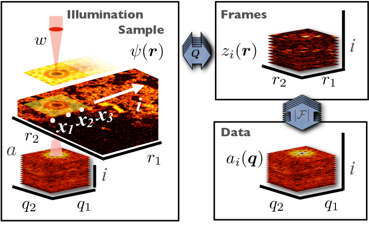
Figure 1: (Left) Experimental geometry in ptychography: An unknown sample with transmission ψ(𝒓)𝜓𝒓\psi(\bm{r}) is rastered through an illuminating beam w(𝒓)𝑤𝒓w(\bm{r}), and a sequence of diffraction measurements |a(i)|2superscriptsubscript𝑎𝑖2|a_{(i)}|^{2} are recorded on an area detector as the sample is rastered around. The point-wise product between illuminating function and sample z(i)(𝒓)=w(𝒓)ψ(𝒓+𝒙(i))subscript𝑧𝑖𝒓𝑤𝒓𝜓𝒓subscript𝒙𝑖z_{(i)}(\bm{r})=w({\bm{r}})\psi({\bm{r}}+{\bm{x}}_{(i)}) -which we refer to as “frame” throuout the paper- is related to the measurement by a Fourier magnitude relationship a(i)=|z(i)|subscript𝑎𝑖subscript𝑧𝑖a_{(i)}=\left|{\cal F}z_{(i)}\right|.

I Introduction

Ptychography was proposed in 1969 to improve the resolution in electron or x-ray microscopy Hoppe ; hegerl ; batesptycho ; spence:book . In a scanning microscope, a small beam is focused onto the sample via a lens, and the transmission is measured in a single-element detector. The image is built up by plotting the transmission as a function of the sample position as it is rastered across the beam. In such microscope, the resolution of the image is given by the beam size. In ptychography, one replaces the single element detector with a two dimensional array detector such as a CCD and measures the intensity distribution at many scattering angles. Each recorded diffraction pattern contains short-spatial Fourier frequency information about features that are smaller than the beam-size, enabling higher resolution. At short wavelengths however it is only possible to measure the intensity of the diffracted light. To reconstruct an image of the object, one needs to retrieve the phase information. With measured amplitude and phase information, a high resolution image can be readily computed, phase contrast imaging becomes possible, and the depth of focus for 3D micro-tomography is no longer a problem. While phase retrieval problems are notoriously difficult to solve numerically, the problem is made tractable in ptychography by using redundant measurements. In practice, multiple views of the same region of the object are recorded by using a small step size -relative to the size of the illuminating beam- when scanning the sample. With high speed detectorspilatus ; fastccd and ever brighter light sources, ptychographic imaging is becoming increasingly popular.

A practical issue in ptychographic reconstruction are the strict requirements of the experimental geometry to achieve high quality data. For example, the need for stable, well controlled coherent illumination of the sample, limited detector speed and response function all contribute to limit the specifications of a ptychographic microscope. New methods to work with unknown illuminations were proposedChapman1996 ; Thibault2008 ; thibault:probe ; pie2 . They are now used to calibrate high quality x-ray optics Kewish2010 ; Honig:11 ; guizar-mirror and space telescopes. More recently, position errorsfienup ; Maiden:2012 ; axel , backgroundthurman2009 ; guizar:bias , noise statistics Thibault-Guizar ; Godard:12 and partially coherent illuminationclark:2011 ; Fienup:93 ; Abbey2008 ; CDIpartialcoherence ; spence-flip , or vibrations have been added to the nonlinear optimization to fit the data.

Existing methods iterate between an object space - an image representing an estimate of the object - and a measurement space given by the measured diffraction frames. For example in the approach first described by fienup , one starts from an estimate of the positions of the illuminating beam and an estimate of the object under study. From this starting point one minimizes the discrepancy with the data using local - gradient based - optimization and obtains a new estimate of the object and positions.

In this paper we introduce an additional optimization step in the measurement space which is -since in ptychographic experiments one records multiple views of the same region of the object - of higher dimensionality than the object space. We form pairwise comparisons between neighboring frames and update the unknown parameters of each diffraction frame so that each frame is consistent with each other.

The approach described in this work achieves accelerated convergence for large scale phase retrieval problems spanning multiple length-scales. We also show that this approach can recover experimental fluctuations over a large range of time-scales.

Notation and background

In a ptychography experiment batesptycho ; rodenburg ; Chapman1996 ; pie1 ; pie2 ; Thibault2008 ; Dierolf (see Fig. 1), a two dimensional small beam with distribution w(𝒓)𝑤𝒓w(\bm{r}) of dimension m×m𝑚𝑚m\times m illuminates an subregion centered at 𝒙(i)subscript𝒙𝑖{\bm{x}}_{(i)} -referred to as frame- of an unknown object of interest ψ𝜓\psi of dimension n×n𝑛𝑛n\times n. Here 0<m<n0𝑚𝑛0<m<n, i=1,,k𝑖1𝑘i=1,\ldots,k, k𝑘k is the number of frames, r>0𝑟0r>0 is a lengthscale (the diffraction limited resolution of the microscope), and

𝒓=(rμ,rν),μ,ν{0,,m1},formulae-sequence𝒓𝑟𝜇𝑟𝜈𝜇𝜈0𝑚1\displaystyle{\bm{r}}=\left(r\mu,r\nu\right),\,\,\mu,\nu\in\{0,\ldots,m-1\},
𝒙(i)=(rμ,rν),μ,ν{0,,nm}.formulae-sequencesubscript𝒙𝑖𝑟superscript𝜇𝑟superscript𝜈superscript𝜇superscript𝜈0𝑛𝑚\displaystyle{\bm{x}}_{(i)}=\left(r\mu^{\prime},r\nu^{\prime}\right),\,\,\mu^{\prime},\nu^{\prime}\in\{0,\ldots,n-m\}.

As 𝒙(i)subscript𝒙𝑖{\bm{x}}_{(i)} is rastered on a typically coarser grid, 𝒓+𝒙(i)𝒓subscript𝒙𝑖\bm{r}+{\bm{x}}_{(i)} spans a finer grid of dimension n×n𝑛𝑛n\times n. Here for simplicity we consider square matrices, and generalization to non-square matrices is straightforward but requires more indices and complicates notation. In other words, we assume that a sequence of k𝑘k diffraction intensity patterns (i)(𝒒)=a(i)2(𝒒)subscript𝑖𝒒superscriptsubscript𝑎𝑖2𝒒{\cal{I}}_{(i)}({\bm{q}})=a_{(i)}^{2}({\bm{q}}) are collected as the position of the object is rastered on the position 𝒙(i)subscript𝒙𝑖{\bm{x}}_{(i)}, where

𝒒=(2πmrμ,2πmrν),μ,ν{0,,m1}.formulae-sequence𝒒2𝜋𝑚𝑟𝜇2𝜋𝑚𝑟𝜈𝜇𝜈0𝑚1{\bm{q}}=\left(\tfrac{2\pi}{mr}\mu,\tfrac{2\pi}{mr}\nu\right),\,\,\mu,\nu\in\{0,\ldots,m-1\}.

The relationship among the amplitude a(i)subscript𝑎𝑖a_{(i)}, the probe w𝑤w and an unknown object ψ𝜓\psi to be estimated can be expressed as follows:

a(i)(𝒒)=|w(𝒓)ψ(𝒓+𝒙(i))|,subscript𝑎𝑖𝒒𝑤𝒓𝜓𝒓subscript𝒙𝑖\displaystyle a_{(i)}({\bm{q}})=\left|{\cal F}w({\bm{r}})\psi({\bm{r}}+{\bm{x}}_{(i)})\right|,
(f)(𝒒)=𝒓ei𝒒𝒓f(𝒓),𝑓𝒒subscript𝒓superscript𝑒𝑖𝒒𝒓𝑓𝒓\displaystyle({\cal F}f)(\bm{q})=\sum_{{\bm{r}}}e^{i{\bm{q}}\cdot{\bm{r}}}f({\bm{r}}),

where the sum over 𝒓𝒓{\bm{r}} is given on all the indices m×m𝑚𝑚m\times m of 𝒓𝒓\bm{r}, and {\cal F} is the two dimensional discrete Fourier transform.

We introduce the illumination operator Q(i)subscript𝑄𝑖Q_{(i)}, i=1,2,,k𝑖12𝑘i=1,2,\cdots,k, associated with 𝒙(i)subscript𝒙𝑖{\bm{x}}_{(i)} that extracts a frame z(i)subscript𝑧𝑖z_{(i)} out of ψ𝜓\psi, and scales the frame point-wise by the illumination function w(𝒓)𝑤𝒓w(\bm{r}) (see Fig. 1):

z(i)(𝒓)=w(𝒓)ψ(𝒓+𝒙(i))=[Q(i)ψ](𝒓),subscript𝑧𝑖𝒓𝑤𝒓𝜓𝒓subscript𝒙𝑖delimited-[]subscript𝑄𝑖𝜓𝒓\displaystyle z_{(i)}({\bm{r}})=w({\bm{r}})\psi({\bm{r}}+{\bm{x}}_{(i)})=[Q_{(i)}\psi]({\bm{r}}),

where z(i)subscript𝑧𝑖z_{(i)} represents the frames extracted from ψ𝜓\psi and multiplied by the probe w(𝒓)𝑤𝒓w({\bm{r}}).

To have a compact representation for numerics, we introduce the following notations. We represent ψ𝜓\psi as a vector of length n2superscript𝑛2n^{2}, that is, ψn2𝜓superscriptsuperscript𝑛2\psi\in\mathbb{C}^{n^{2}}. The moving beam associated with the illumination function w(𝒓)𝑤𝒓w(\bm{r}) can be represented as an m2×n2superscript𝑚2superscript𝑛2m^{2}\times n^{2} sparse “illumination matrix” associated with the illumination operator, which is again denoted as Q(i)subscript𝑄𝑖Q_{(i)}. To express Q(i)subscript𝑄𝑖Q_{(i)} in the matrix form, we introduce a restriction matrix R(i)subscript𝑅𝑖R_{(i)}, which restricts the n×n𝑛𝑛n\times n region onto the m×m𝑚𝑚m\times m subregion centered at 𝒙(i)subscript𝒙𝑖{\bm{x}}_{(i)}, that is,

Q(i)=diag(w)R(i).subscript𝑄𝑖diag𝑤subscript𝑅𝑖Q_{(i)}=\text{diag}(w)R_{(i)}.

The relationship between the diffraction measurements collected in a ptychography experiment and the unknown object to be recovered can be represented compactly as:

𝒂𝒂\displaystyle\bm{a} =\displaystyle= |𝑭𝑸ψ|,𝑭𝑸𝜓\displaystyle|{\bm{F}}{\bm{Q}}\psi|, (1)

if we stack the diffraction measurements a(i)subscript𝑎𝑖a_{(i)} into a long vector 𝒂𝒂\bm{a}, and define various matrices as follows:

𝒂𝒂\displaystyle\bm{a} =\displaystyle= (a(1)a(k)),𝑸=(Q(1)Q(k)),subscript𝑎1subscript𝑎𝑘𝑸subscript𝑄1subscript𝑄𝑘\displaystyle\left(\begin{array}[]{c}a_{(1)}\\ \vdots\\ a_{(k)}\end{array}\right),\,{\bm{Q}}=\left(\begin{array}[]{c}Q_{(1)}\\ \vdots\\ Q_{(k)}\end{array}\right),\, (8)
𝒛𝒛\displaystyle{\bm{z}} =\displaystyle= (z(1)z(k)),𝑭=().subscript𝑧1subscript𝑧𝑘𝑭missing-subexpressionmissing-subexpressionmissing-subexpressionmissing-subexpressionmissing-subexpressionmissing-subexpression\displaystyle\left(\begin{array}[]{c}z_{(1)}\\ \vdots\\ z_{(k)}\end{array}\right),\,\bm{F}=\left(\begin{array}[]{ccc}{\cal F}\\ &\ddots&\\ &&{\cal F}\end{array}\right)\,. (15)

We call the domain of 𝑸𝑸{\bm{Q}} the object space, and the range of 𝑭𝑸𝑭𝑸\bm{F}\bm{Q} the measurement space.

Geometrically, 𝑸𝑸{\bm{Q}} is the matrix that extracts k𝑘k frames out of an object ψ𝜓\psi and multiplies them by the probe w𝑤w; 𝑸superscript𝑸{\bm{Q}}^{\ast} is the conjugate transpose that merges k𝑘k frames onto the object space; in addition, 𝑸𝑸superscript𝑸𝑸{\bm{Q}}^{\ast}{\bm{Q}} can be viewed as the normalization factor given by the sum of the illumination functions. In particular, by a direct calculation, 𝑸𝑸superscript𝑸𝑸{\bm{Q}}^{\ast}{\bm{Q}} is a n×n𝑛𝑛n\times n diagonal matrix whose l𝑙l-th diagonal entry is k:l=𝒙k+𝒓k|w(𝒓k)|2subscript:𝑘𝑙subscript𝒙𝑘subscript𝒓𝑘superscript𝑤subscript𝒓𝑘2\sum_{k:\,l={\bm{x}}_{k}+{\bm{r}}_{k}}|w({\bm{r}}_{k})|^{2}, where we abuse the notation by using l𝑙l to indicate the point on the object space. Physically l𝑙l is the index of the grid point on the unknown object of interest which is covered by the point 𝒓ksubscript𝒓𝑘{\bm{r}}_{k} of the k𝑘k-th illumination window. See table 1 for the relationship between probe w𝑤w, translation 𝒙(i)subscript𝒙𝑖{\bm{x}}_{(i)}, Q(i)subscript𝑄𝑖Q_{(i)} and 𝑸𝑸{\bm{Q}}.

Q(i)ψsubscript𝑄𝑖𝜓Q_{(i)}\psi diag(w)R(i)ψdiag𝑤subscript𝑅𝑖𝜓\text{diag}(w)R_{(i)}\psi
Q(i)z(i)superscriptsubscript𝑄𝑖subscript𝑧𝑖Q_{(i)}^{\ast}z_{(i)} R(i)diag(conj(w))z(i)superscriptsubscript𝑅𝑖diagconj𝑤subscript𝑧𝑖R_{(i)}^{*}\text{diag}(\mathrm{conj}(w))z_{(i)}
𝑸𝒛superscript𝑸𝒛{\bm{Q}}^{\ast}{\bm{z}} iR(i)diag(conj(w))z(i)subscript𝑖superscriptsubscript𝑅𝑖diagconj𝑤subscript𝑧𝑖\sum_{i}R_{(i)}^{*}\text{diag}(\mathrm{conj}(w))z_{(i)}
elT𝑸𝑸eksuperscriptsubscript𝑒𝑙𝑇superscript𝑸𝑸subscript𝑒𝑘e_{l}^{T}{\bm{Q}}^{\ast}{\bm{Q}}e_{k} 𝒙k+𝒓k=l|w(𝒓k)|2δl,ksubscriptsubscript𝒙𝑘subscript𝒓𝑘𝑙superscript𝑤subscript𝒓𝑘2subscript𝛿𝑙𝑘\sum_{{\bm{x}}_{k}+{\bm{r}}_{k}=l}|w({\bm{r}}_{k})|^{2}\delta_{l,k}
elT(𝑸𝑸)1𝑸𝒛superscriptsubscript𝑒𝑙𝑇superscriptsuperscript𝑸𝑸1superscript𝑸𝒛e_{l}^{T}({\bm{Q}}^{\ast}{\bm{Q}})^{-1}{\bm{Q}}^{\ast}{\bm{z}} elTiR(i)diag(conj(w))z(i)𝒙k+𝒓k=l|w(𝒓k)|2superscriptsubscript𝑒𝑙𝑇subscript𝑖superscriptsubscript𝑅𝑖diagconj𝑤subscript𝑧𝑖subscriptsubscript𝒙𝑘subscript𝒓𝑘𝑙superscript𝑤subscript𝒓𝑘2\frac{e_{l}^{T}\sum_{i}R_{(i)}^{*}\text{diag}(\mathrm{conj}(w))z_{(i)}}{\sum_{{\bm{x}}_{k}+{\bm{r}}_{k}=l}|w({\bm{r}}_{k})|^{2}}
P𝑭𝒂(i)z(i)superscriptsubscript𝑃𝑭subscript𝒂𝑖subscript𝑧𝑖P_{\bm{F}}^{\bm{a}_{(i)}}z_{(i)} 𝒒ei𝒒𝒓𝒓ei𝒒𝒓z(i)(𝒓)|𝒓ei𝒒𝒓z(i)(𝒓)|𝒂(i)subscript𝒒superscript𝑒𝑖𝒒𝒓subscript𝒓superscript𝑒𝑖𝒒𝒓subscript𝑧𝑖𝒓subscript𝒓superscript𝑒𝑖𝒒𝒓subscript𝑧𝑖𝒓subscript𝒂𝑖\sum_{{\bm{q}}}e^{-i{\bm{q}}\cdot{\bm{r}}}\frac{\sum_{{\bm{r}}}e^{i{\bm{q}}\cdot{\bm{r}}}z_{(i)}({\bm{r}})}{|\sum_{{\bm{r}}}e^{i{\bm{q}}\cdot{\bm{r}}}z_{(i)}({\bm{r}})|}\bm{a}_{(i)}
Table 1: Linear algebra notation. Here elsubscript𝑒𝑙e_{l} is the unit n×1𝑛1n\times 1 vector with the l𝑙l-th entry 111 and δ𝛿\delta is the Kronecker delta. The division is understood as an element-wise operation. The operator P𝑭𝒂(i)superscriptsubscript𝑃𝑭subscript𝒂𝑖P_{\bm{F}}^{\bm{a}_{(i)}} is defined in (22)

The objective of the ptychographic reconstruction problem is to find ψ𝜓\psi given 𝒂𝒂\bm{a} from (Eq. 1). This is often formulated using a “divide and conquer” approach referred to as projection algorithms, iterative transform methods, or alternating direction methods ZWen . One formulates the relationship (Eq. 1) as:

𝒂𝒂\displaystyle\bm{a} =\displaystyle= |𝑭𝒛|,𝑭𝒛\displaystyle|{\bm{F}}{\bm{z}}|, (16)
𝒛𝒛\displaystyle{\bm{z}} =\displaystyle= 𝑸ψ.𝑸𝜓\displaystyle{\bm{Q}}\psi. (17)

These algorithms are often defined in terms of two projection operators PF𝒂superscriptsubscript𝑃𝐹𝒂P_{F}^{\bm{a}} and PQsubscript𝑃𝑄P_{Q} that project onto the solution z𝑧z to Eqs. (16 and 17) that is closest to the current estimate described in Section II.

Alternative approaches include formulating the problem as:

minψ𝒂|𝑭𝑸ψ|subscript𝜓norm𝒂𝑭𝑸𝜓\displaystyle\min_{\psi}\|\bm{a}-|{\bm{F}}{\bm{Q}}\psi|\| (18)

and solve it by standard unconstrained minimization algorithms such as conjugate gradient, Newton and quasi-Newton methods fienup ; lbnlptyco ; Thibault-Guizar . Efficient projection operators can be used if we formulate Eq. 18 using the frames 𝒛𝒛{\bm{z}} as slack variables as discussed in Section II and solve:

min𝒛𝒂|𝑭𝒛|subscript𝒛norm𝒂𝑭𝒛\displaystyle\min_{\begin{subarray}{c}{\bm{z}}\end{subarray}}\|\bm{a}-|\bm{F}{\bm{z}}|\| (19)

with the conditions that 𝒛𝒛{\bm{z}} satisfies Eq. (17) using projected gradient, Newton and quasi-Newton methodslbnlptyco ; lbnlptycho1 . .

Another approach uses a n2×n2superscript𝑛2superscript𝑛2n^{2}\times n^{2} phase-space described in terms of a “Wigner Distribution” functionbatesptycho ; Chapman1996 . More recently phaselift ; Ohlsson ; candes11 a convex relaxation of the quadratic problem is obtained by lifting to an n2×n2superscript𝑛2superscript𝑛2n^{2}\times n^{2} space and minimizing the rank of the matrix

Main results

The main contribution of this paper is the introduction of an additional optimization step in the measurement space, which with a dimensionality of km2𝑘superscript𝑚2km^{2}, is larger than the object space, n2superscript𝑛2n^{2}. It is aimed to deal with fluctuating intensities, position errors, poor calibration using multiplexing illumination, and an unknown offset (background) for every pixel but constant throughout the acquisition (or vice versa). Specifically, instead of solving Eq. (18), we wish to minimize the gap between the measurement space and the smaller object space:

min𝒛,|𝑭𝒛|=𝒂[IP𝑸]𝒛,subscript𝒛𝑭𝒛𝒂normdelimited-[]𝐼subscript𝑃𝑸𝒛\displaystyle\min_{\begin{subarray}{c}{\bm{z}},|\bm{F}{\bm{z}}|=\bm{a}\end{subarray}}\|[I-P_{\bm{Q}}]{\bm{z}}\|, (20)

where I𝐼I is the identity operator and PQsubscript𝑃𝑄P_{Q} represents a projection onto the object space and will be described in the following section.

Recently it was proposed to use maxcut algorithms to solve a similar problem Waldspurger . Here we approach the problem differently. We start from the redundant measurement space and compute pairwise comparison between frames before merging into the object space.

In section III we consider the case that the diffraction measurement a(i)subscript𝑎𝑖a_{(i)} is contaminated (i.e. multiplied) by a unknown scalar factor ω(i)subscript𝜔𝑖\omega_{(i)}. We encounter this problem if the intensity or integration time of the incident beam is unknown. If we fix the relative amplitude and phase within every frame z(i)subscript𝑧𝑖z_{(i)} and minimize the gap Eq. (20) with respect to the vector 𝝎𝝎\bm{\omega} for a given 𝒛𝒛{\bm{z}}, we can express Eq. (20) as:

min𝝎subscript𝝎\displaystyle\min_{\bm{\omega}} 𝝎H𝝎superscript𝝎𝐻𝝎\displaystyle\bm{\omega}^{\ast}H\bm{\omega} (21)
Hi,jsubscript𝐻𝑖𝑗\displaystyle H_{i,j} =\displaystyle= z(i)(δi,jIQ(i)Q(j)eiT(𝑸𝑸)ej)z(j),superscriptsubscript𝑧𝑖subscript𝛿𝑖𝑗𝐼subscript𝑄𝑖superscriptsubscript𝑄𝑗superscriptsubscript𝑒𝑖𝑇superscript𝑸𝑸subscript𝑒𝑗subscript𝑧𝑗\displaystyle z_{(i)}^{\ast}\left(\delta_{i,j}I-\tfrac{Q_{(i)}Q_{(j)}^{\ast}}{e_{i}^{T}({\bm{Q}}^{\ast}{\bm{Q}})e_{j}}\right)z_{(j)},

where the k×k𝑘𝑘k\times k matrix H𝐻H is calculated by computing the pairwise dot product between overlapping frames. While this problem arises from the need to account for intensity fluctuations, it turns out to be a useful technique to improve the convergence rate for large scale problems. The phase vector obtained by normalizing 𝝎𝝎\bm{\omega} enables us to adjust for the relative phase between frames and accelerate the rate of convergence in iterative algorithms.

We use a similar approach to optimize perturbations of the illumination matrix 𝑸𝑸{\bm{Q}}: the position among frames (Section IV). Alternative approaches optimizing the positions from the reduced object space have been proposed by others Maiden:2012 ; fienup . By minimizing the gap between measurement space and constraint, we obtain a first order correction formula that relies on pairwise scalar products between neighboring frames. We expect a method based on pairwise comparsions to work well in large scale problems when long range position drifts may arise.

In Section VI we report the following numerical results:

  • Exact reconstruction with intensity fluctuation given by the coefficients ω(i)subscript𝜔𝑖\omega_{(i)} (see Fig. 4).

  • Accelerated convergence (Fig. 5) even when no intensity fluctuation is present in the data (Table 3)

  • Exact reconstruction with multiplexing using 4 simultaneous illuminations adding incoherently on the detector, with perturbation of the amplitudes (Fig. 6)

  • Position recovery (Figs. 7) of the illuminating probe.

  • Joint reconstruction of the sample and fluctuating background noise independent from the sample (Figs. 8,9).

  • Exact reconstruction with missing (corrupted) data entries (see Fig. 12,12).

In the following section II we will describe the standard operators commonly used in the literature.

II Standard Projection algorithms

The projection operator PF𝒂subscriptsuperscript𝑃𝒂𝐹P^{\bm{a}}_{F} mentioned in the previous section is often known as the Fourier magnitude projection operator. Applying this operator to a vector 𝒛𝒛{\bm{z}} yields

PF𝒂𝒛=𝑭(𝑭𝒛|𝑭𝒛|𝒂).superscriptsubscript𝑃𝐹𝒂𝒛superscript𝑭𝑭𝒛𝑭𝒛𝒂\displaystyle P_{F}^{\bm{a}}{\bm{z}}={\bm{F}}^{\ast}\left(\frac{{\bm{F}}{\bm{z}}}{|{\bm{F}}{\bm{z}}|}\cdot\bm{a}\right).\ \ (22)

where division and multiplication are intended as element-wise operations. It is easy to verify that |PF𝒂𝒛|=|𝒂|subscriptsuperscript𝑃𝒂𝐹𝒛𝒂|P^{\bm{a}}_{F}{\bm{z}}|=|\bm{a}| and therefore PF𝒂𝒛subscriptsuperscript𝑃𝒂𝐹𝒛P^{\bm{a}}_{F}{\bm{z}} satisfies Eq. (16) for any 𝒛𝒛{\bm{z}}. We mention that PF𝒂subscriptsuperscript𝑃𝒂𝐹P^{\bm{a}}_{F} is a projection in the sense that

PF𝒂𝒛=argmin𝒛¯𝒛(i)𝒛¯(i),superscriptsubscript𝑃𝐹𝒂𝒛subscript¯𝒛normsubscript𝒛𝑖subscript¯𝒛𝑖\displaystyle P_{F}^{\bm{a}}{\bm{z}}=\arg\min_{\bar{\bm{z}}}\|{\bm{z}}_{(i)}-\bar{\bm{z}}_{(i)}\|, (23)
subject to |𝑭𝒛¯|=𝒂,subject to 𝑭¯𝒛𝒂\displaystyle\text{ subject to }|{\bm{F}}\bar{\bm{z}}|=\bm{a},\,

where \|\,\| denotes the Euclidean norm. The matrix 𝑸𝑸{\bm{Q}} defines an orthogonal projection operator P𝑸subscript𝑃𝑸P_{\bm{Q}} that projects any vector in km2superscript𝑘superscript𝑚2\mathbb{C}^{km^{2}} onto the range of 𝑸𝑸{\bm{Q}}:

PQ=𝑸(𝑸𝑸)1𝑸,subscript𝑃𝑄𝑸superscriptsuperscript𝑸𝑸1superscript𝑸P_{Q}={\bm{Q}}({\bm{Q}}^{\ast}{\bm{Q}})^{-1}{\bm{Q}}^{\ast}, (24)

when (𝑸𝑸)1superscriptsuperscript𝑸𝑸1({\bm{Q}}^{\ast}{\bm{Q}})^{-1} exists. An alternative formulation uses projection operators that apply on the Fourier frames 𝒛^=𝑭𝒛bold-^𝒛𝑭𝒛\bm{\hat{z}}=\bm{F}{\bm{z}}:

P~𝑸subscript~𝑃𝑸\displaystyle\tilde{P}_{\bm{Q}} =\displaystyle= 𝑭P𝑸𝑭,P~F𝒂=𝑭PF𝒂𝑭.𝑭subscript𝑃𝑸superscript𝑭superscriptsubscript~𝑃𝐹𝒂𝑭superscriptsubscript𝑃𝐹𝒂superscript𝑭\displaystyle\bm{F}P_{\bm{Q}}\bm{F}^{\ast},\quad\tilde{P}_{F}^{\bm{a}}=\bm{F}P_{F}^{\bm{a}}\bm{F}^{\ast}.

Line search stratrategies to solve Eq. (23) can be implemented more efficiently using this formulationlbnlptyco .

In the simple alternating projection algorithm, the approximation to the solutions of (Eqs. (16) and (17)) are updated by:

𝒛()superscript𝒛\displaystyle{\bm{z}}^{(\ell)} =\displaystyle= [P𝑸PF𝒂]𝒛(1),delimited-[]subscript𝑃𝑸subscriptsuperscript𝑃𝒂𝐹superscript𝒛1\displaystyle\left[P_{{\bm{Q}}}P^{\bm{a}}_{F}\right]{\bm{z}}^{(\ell-1)}, (25)

where typically the initial guess 𝒛(0)superscript𝒛0{\bm{z}}^{(0)} is a random vector. Clearly PF𝒂superscriptsubscript𝑃𝐹𝒂P_{F}^{\bm{a}} from (23) forces 𝒛(1)superscript𝒛1{\bm{z}}^{(\ell-1)} to have the right amplitude in the Fourier domain, and P𝑸subscript𝑃𝑸P_{{\bm{Q}}} forces PF𝒂𝒛(1)superscriptsubscript𝑃𝐹𝒂superscript𝒛1P_{F}^{\bm{a}}{\bm{z}}^{(\ell-1)} to be located in the range of 𝑸𝑸{\bm{Q}}. We note that the projector P𝑸subscript𝑃𝑸P_{\bm{Q}} can be expressed by computing the running estimate of ψ𝜓\psi denoted as ψ()superscript𝜓\psi^{(\ell)}

ψ()superscript𝜓\displaystyle\psi^{(\ell)} =\displaystyle= argminψPF𝒂𝒛(1)𝑸ψ,subscript𝜓normsuperscriptsubscript𝑃𝐹𝒂superscript𝒛1𝑸𝜓\displaystyle\arg\min_{\psi}\|P_{F}^{\bm{a}}\bm{z}^{(\ell-1)}-{\bm{Q}}\psi\|, (26)

which is solved by taking Eq. (24) into account:

ψ()superscript𝜓\displaystyle\psi^{(\ell)} =\displaystyle= [(𝑸𝑸)1𝑸]PF𝒂𝒛(1),delimited-[]superscriptsuperscript𝑸𝑸1superscript𝑸superscriptsubscript𝑃𝐹𝒂superscript𝒛1\displaystyle\left[({\bm{Q}}^{\ast}{\bm{Q}})^{-1}{\bm{Q}}^{\ast}\right]{P_{F}^{\bm{a}}}{\bm{z}}^{(\ell-1)}, (27)

when (𝑸𝑸)1superscriptsuperscript𝑸𝑸1({\bm{Q}}^{\ast}{\bm{Q}})^{-1} exists. Notice that P𝑸PF𝒂𝒛(1)=𝑸ψ()subscript𝑃𝑸superscriptsubscript𝑃𝐹𝒂superscript𝒛1𝑸superscript𝜓P_{{\bm{Q}}}P_{F}^{\bm{a}}{\bm{z}}^{(\ell-1)}={\bm{Q}}\psi^{(\ell)}.

We mention two practical issues regarding the updating steps (26) and (23). First, since (𝑸𝑸)1superscriptsuperscript𝑸𝑸1({\bm{Q}}^{\ast}{\bm{Q}})^{-1} may not exist, one may introduce a regularization factor ϵitalic-ϵ\epsilon into (26) and update the running estimate as:

ψ()=(𝑸𝑸+ϵ)1(𝑸PF𝒂𝒛(1)+ϵψ(1)).superscript𝜓superscriptsuperscript𝑸𝑸italic-ϵ1superscript𝑸superscriptsubscript𝑃𝐹𝒂superscript𝒛1italic-ϵsuperscript𝜓1\displaystyle\psi^{(\ell)}=({\bm{Q}}^{\ast}{\bm{Q}}+\epsilon)^{-1}\left({\bm{Q}}^{\ast}P_{F}^{\bm{a}}{\bm{z}}^{(\ell-1)}+\epsilon\psi^{(\ell-1)}\right). (28)

with typically ψ(0)=0superscript𝜓00\psi^{(0)}=0. ϵitalic-ϵ\epsilon is a regularization factor that leaves unchanged the entries that are never illuminated, and gradually reduces the correction from ψ(1)superscript𝜓1\psi^{(\ell-1)} where the sum of the illuminating probe intensities is small. If we replace Eq. (27) by Eq. (28) we obtain an operator that is no longer a projection operator but can be viewed as a relaxed projection.

If the entries of a(i)(𝒒)subscript𝑎𝑖𝒒a_{(i)}({\bm{q}}) are corrupted by gaussian random noise with known variance 𝝈(i)2(𝒒)superscriptsubscript𝝈𝑖2𝒒\bm{\sigma}_{(i)}^{2}({\bm{q}}), which is expressed as a m2superscript𝑚2m^{2} long column vector, one may replace Eq. (23) modifying PF𝒂superscriptsubscript𝑃𝐹𝒂P_{F}^{\bm{a}} with

PF(𝒂,σ)𝒛=𝑭(𝑭𝒛|𝑭𝒛|𝒂+|𝑭𝒛|𝝈21+𝝈2),superscriptsubscript𝑃𝐹𝒂𝜎𝒛superscript𝑭𝑭𝒛𝑭𝒛𝒂𝑭𝒛superscript𝝈21superscript𝝈2\displaystyle P_{F}^{(\bm{a},\sigma)}{\bm{z}}=\bm{F}^{*}\left(\frac{\bm{F}{\bm{z}}}{|\bm{F}{\bm{z}}|}\cdot{\frac{\bm{a}+|\bm{F}{\bm{z}}|\bm{\sigma}^{2}}{1+\bm{\sigma}^{2}}}\right), (29)

where 𝝈𝝈\bm{\sigma} is viewed as a regularization factor that leaves unchanged the entries of 𝒛𝒛{\bm{z}} when the data entries are completely corrupted (𝝈2superscript𝝈2\bm{\sigma}^{2}\to\infty). Clearly 𝒂+|𝑭𝒛|𝝈21+𝝈21|𝑭𝒛|1𝒂𝑭𝒛superscript𝝈21superscript𝝈21𝑭𝒛1\tfrac{\bm{a}+|\bm{F}{\bm{z}}|\bm{\sigma}^{2}}{1+\bm{\sigma}^{2}}\tfrac{1}{|\bm{F}{\bm{z}}|}\to 1 when 𝝈2superscript𝝈2\bm{\sigma}^{2}\to\infty. When 𝝈20superscript𝝈20\bm{\sigma}^{2}\to 0, (Eq 29) reverts to the regular projection operator (Eq. 22).

The simple alternating projection algorithm can be viewed as the projected steepest descent algorithms. Projected conjugate gradient methods have also been proposed in fienup ; lbnlptyco ; Thibault-Guizar to accelerate convergence rate.

A number of heuristic first order algorithms have been proposed that outperform the simple algorithms, a few examples are given in Tab. 2, with β[0,1]𝛽01\beta\in[0,1] is a relaxation parameter. Very recently, an alternating direction method (ADM) was proposed to work with a special augmented Lagrangian function ZWen . This function is minimized by applying a block coordinate descent schemezwen2 (or alternating search directions) akin to these projection operators.

projection algorithm updating formula 𝒛(+1)=superscript𝒛1absent{\bm{z}}^{(\ell+1)}=
Alternating Projection hio [PQPF]𝒛()delimited-[]subscript𝑃𝑄subscript𝑃𝐹superscript𝒛\left[P_{Q}P_{F}\right]{\bm{z}}^{(\ell)}
HIO hio [PQPF+(IPQ)(IβPF)]𝒛()delimited-[]subscript𝑃𝑄subscript𝑃𝐹𝐼subscript𝑃𝑄𝐼𝛽subscript𝑃𝐹superscript𝒛\left[P_{Q}P_{F}+(I-P_{Q})(I-\beta P_{F})\right]{\bm{z}}^{(\ell)}
Difference Map Thibault2008 [PFPQ+(IPF)(IβPQ)]𝒛()delimited-[]subscript𝑃𝐹subscript𝑃𝑄𝐼subscript𝑃𝐹𝐼𝛽subscript𝑃𝑄superscript𝒛\left[P_{F}P_{Q}+(I-P_{F})(I-\beta P_{Q})\right]{\bm{z}}^{(\ell)}
RAARraar [2βPQPF+(12β)PF+β(PQI)]𝒛()delimited-[]2𝛽subscript𝑃𝑄subscript𝑃𝐹12𝛽subscript𝑃𝐹𝛽subscript𝑃𝑄𝐼superscript𝒛\left[2\beta P_{Q}P_{F}+(1-2\beta)P_{F}+\beta(P_{Q}-I)\right]{\bm{z}}^{(\ell)}
Table 2: Popular fix-point algorithms used in phase retrieval. HIO: hybrid input-output algorithm. RAAR: Relaxed averaged alternating reflections algorithm.

III Fluctuating intensities, and augmented phase retrieval

Intensity fluctuations can be accounted for by introducing a scalar scaling factor ωisubscript𝜔𝑖\omega_{i}\in\mathbb{C} multiplying every (m2superscript𝑚2m^{2}) pixel of a diffraction frame. This can be expressed in various forms (frame by frame or all at once) as:

|(z(i))||ω(i)|subscript𝑧𝑖subscript𝜔𝑖\displaystyle|({\cal F}z_{(i)})|\cdot|\omega_{(i)}| =\displaystyle= a(i),isubscript𝑎𝑖for-all𝑖\displaystyle a_{(i)},\quad\forall i (30)
|diag(𝑭𝒛)𝑩𝝎|diag𝑭𝒛𝑩𝝎\displaystyle|{\mbox{diag}\left(\bm{F}{\bm{z}}\right)}\bm{B}\bm{\omega}| =\displaystyle= 𝒂,(𝑩)i,j=δi,j1m2,𝒂subscript𝑩𝑖𝑗subscript𝛿𝑖𝑗subscript1superscript𝑚2\displaystyle\bm{a},\quad(\bm{B})_{i,j}=\delta_{i,j}1_{m^{2}}, (31)

where 𝝎=[ω1,,ωk]k𝝎subscript𝜔1subscript𝜔𝑘superscript𝑘\bm{\omega}=[\omega_{1},\ldots,\omega_{k}]\in\mathbb{C}^{k} and 𝑩𝑩\bm{B} is a k×k𝑘𝑘k\times k diagonal block matrix with the diagonal entry 1m2subscript1superscript𝑚21_{m^{2}}, which is the m2×1superscript𝑚21m^{2}\times 1 matrix with 111 in all entries. In other words, 𝑩𝑩\bm{B} copies the scalar factors ωisubscript𝜔𝑖\omega_{i} before multiplying by 𝑭𝒛𝑭𝒛\bm{F}{\bm{z}}. In practice ωisubscript𝜔𝑖\omega_{i} is unknown and needs to be estimated. If we know 𝒛𝒛{\bm{z}} or its approximation, to estimate ωisubscript𝜔𝑖\omega_{i}, we find the vector 𝝎𝝎\bm{\omega} that minimizes the gap with the object space:

argmin𝝎subscript𝝎\displaystyle\arg\min_{\bm{\omega}} (IP𝑸)diag(𝒛)𝑩ω2.superscriptnorm𝐼subscript𝑃𝑸diag𝒛𝑩𝜔2\displaystyle\left\|(I-P_{\bm{Q}})\mbox{diag}\left({\bm{z}}\right)\bm{B}\omega\right\|^{2}. (32)

We can write Eq. (32) as:

argmin𝝎𝝎H𝝎,subscript𝝎superscript𝝎𝐻𝝎\displaystyle\arg\min_{\bm{\omega}}\bm{\omega}^{\ast}H\bm{\omega}, (33)
Hi,jsubscript𝐻𝑖𝑗\displaystyle H_{i,j} =\displaystyle= 𝟏Tdiag(z(i))(δi,jIQ(i)Q(j)eiT(𝑸𝑸)ej)diag(z(j))𝟏,superscript1𝑇diagsuperscriptsubscript𝑧𝑖subscript𝛿𝑖𝑗𝐼subscript𝑄𝑖superscriptsubscript𝑄𝑗superscriptsubscript𝑒𝑖𝑇superscript𝑸𝑸subscript𝑒𝑗diagsubscript𝑧𝑗1\displaystyle\bm{1}^{T}\mbox{diag}\left(z_{(i)}^{\ast}\right)\left(\delta_{i,j}I-\frac{Q_{(i)}Q_{(j)}^{\ast}}{e_{i}^{T}({\bm{Q}}^{\ast}{\bm{Q}})e_{j}}\right)\mbox{diag}\left(z_{(j)}\right)\bm{1},
=\displaystyle= z(i)(δi,jIQ(i)Q(j)eiT(𝑸𝑸)ej)z(j),superscriptsubscript𝑧𝑖subscript𝛿𝑖𝑗𝐼subscript𝑄𝑖superscriptsubscript𝑄𝑗superscriptsubscript𝑒𝑖𝑇superscript𝑸𝑸subscript𝑒𝑗subscript𝑧𝑗\displaystyle{z_{(i)}^{\ast}}\left(\delta_{i,j}I-\frac{Q_{(i)}Q_{(j)}^{\ast}}{e_{i}^{T}({\bm{Q}}^{\ast}{\bm{Q}})e_{j}}\right)z_{(j)},

where the k×k𝑘𝑘k\times k matrix H𝐻H is computed by performing the scalar product between every pair of overlapping frames. We can eliminate the trivial solution 𝝎=0𝝎0\bm{\omega}=0 by setting an additional constraint such as 𝝎𝝎\sum\bm{\omega}, or 𝝎norm𝝎\|\bm{\omega}\|=constant. A simple way to solve this problem (see appendix A) is to start with 𝟏1\bm{1} as our first guess for ω𝜔\omega and solve:

H𝝎=α𝟏,𝐻𝝎𝛼1H\bm{\omega}=\alpha\bm{1},\quad (34)

where α𝛼\alpha is chosen to normalize the average flux 𝝎/𝟏norm𝝎norm1\|\bm{\omega}\|/\|\bm{1}\|.

In order to take the intensity fluctuation problem into account while applying the projection algorithm (16) and (17), we introduce the following solution. First, we replace the operator P𝑸subscript𝑃𝑸P_{\bm{Q}} used in the standard projection algorithms listed in Table 2 by an augmented projection operator P𝑸𝝎superscriptsubscript𝑃𝑸𝝎P_{\bm{Q}}^{\bm{\omega}} defined as:

P𝑸𝝎=D𝝎1P𝑸D𝝎,D𝝎=diag(𝝎),formulae-sequencesuperscriptsubscript𝑃𝑸𝝎subscriptsuperscript𝐷1𝝎subscript𝑃𝑸subscript𝐷𝝎subscript𝐷𝝎diag𝝎P_{{\bm{Q}}}^{\bm{\omega}}=D^{-1}_{\bm{\omega}}P_{\bm{Q}}D_{\bm{\omega}},\quad D_{\bm{\omega}}=\mbox{diag}\left(\bm{\omega}\right), (35)

where 𝝎𝝎\bm{\omega} is the solution to Eq.(33) or Eq.(34). An alternative modification is to recompute the normalization factor 𝑸𝑸superscript𝑸𝑸\bm{Q}^{\ast}\bm{Q} with the scaling factors |ωi|2superscriptsubscript𝜔𝑖2|\omega_{i}|^{2}. This yields an orthogonal projection:

P¯𝑸𝝎=𝑸𝝎(𝑸𝝎𝑸𝝎)1𝑸𝝎,𝑸𝝎=D𝝎1𝑸formulae-sequencesuperscriptsubscript¯𝑃𝑸𝝎subscript𝑸𝝎superscriptsubscriptsuperscript𝑸𝝎subscript𝑸𝝎1superscriptsubscript𝑸𝝎subscript𝑸𝝎superscriptsubscript𝐷𝝎1𝑸\bar{P}_{{\bm{Q}}}^{\bm{\omega}}={\bm{Q}}_{\bm{\omega}}\left({\bm{Q}}^{\ast}_{\bm{\omega}}{\bm{Q}}_{\bm{\omega}}\right)^{-1}{\bm{Q}}_{\bm{\omega}}^{\ast},\quad{\bm{Q}}_{\bm{\omega}}=D_{\bm{\omega}}^{-1}{\bm{Q}} (36)

When no intensity fluctuations are present, we normalize 𝝎𝝎\bm{\omega} and replace D𝝎subscript𝐷𝝎D_{\bm{\omega}} with:

D^ω=diag(𝝎|𝝎|).subscript𝐷bold-^absent𝜔diag𝝎𝝎D_{\bm{\hat{}}\omega}=\mbox{diag}\left(\frac{\bm{\omega}}{|\bm{\omega}|}\right).

Although the construction of P𝑸𝝎superscriptsubscript𝑃𝑸𝝎P_{{\bm{Q}}}^{\bm{\omega}} is motivated by the need to account for intensity fluctuations among different diffraction frames in the measured data, it turns out to be a useful technique for accelerating the convergence of projection algorithms even when no intensity fluctuation is present in the data. The minimization problem in (Eq. 32) is similar to the phase problem of how to merge frames 𝒛(i)subscript𝒛𝑖{\bm{z}}_{(i)} with unknown phase factor 𝝎𝝎\bm{\omega}, which can be written as:

argmin𝝎,|ωi|=1𝝎H𝝎.subscript𝝎subscript𝜔𝑖1𝝎𝐻𝝎\arg\min_{\bm{\omega},|\omega_{i}|=1}\bm{\omega}H\bm{\omega}. (37)

Replacing the condition |𝝎|=𝟏𝝎1|\bm{\omega}|=\bm{1} with weaker conditions such as 𝝎𝝎\sum\bm{\omega} or 𝝎=norm𝝎absent\|\bm{\omega}\|=constant enables us to solve this problem more efficiently. A similar approach is discussed in singer .

The problem of the incoherent superposition of different signals can be treated in a similar way.

III.1 Multiplexing and incoherent measurements

The incoherent measurement model is as follows. We consider zisubscript𝑧𝑖z_{i} the highly redundant set of frames generated for all the positions of the illumination function during an exposure. For example, a single exposure a(i)subscript𝑎𝑖a_{(i)} may represents the sum of the intensities generated by an illumination beam that translates during the exposure, or may represent a binned sample of a continuous signal. Assume we have k𝑘k redundant measurement 𝒛(i)subscript𝒛𝑖\bm{z}_{(i)}, where i=1,,k𝑖1𝑘i=1,\ldots,k. The incoherent measurement is introduced by summing s<k𝑠𝑘s<k illumination windows according to a weight factor, where we assume k/s𝑘𝑠k/s is an integer for convenience. The weight factor, or the integration time, for each frame, is represented by |𝝎|2superscript𝝎2|\bm{\omega}|^{2}. In particular, the redundant set of frames z(i)subscript𝑧𝑖z_{(i)} is not measured directly; instead it is multiplied by a known averaging operator, which is expressed as |𝝎|2superscript𝝎2|\bm{\omega}|^{2} and a (k/s)m2×km2𝑘𝑠superscript𝑚2𝑘superscript𝑚2(k/s)m^{2}\times km^{2} real matrix 𝛀𝛀\bm{\Omega} with all non-zero entries 111. Geometrically, 𝛀𝛀\bm{\Omega} groups the frames, which are weighted by |𝝎|2superscript𝝎2|\bm{\omega}|^{2}, and then the weighted frames in each group are summed. The incoherent measurement can thus be expressed by modifying (31):

𝒂2superscript𝒂2\displaystyle\bm{a}^{2} =\displaystyle= 𝛀(|𝑭𝒛|2𝑩|ω|2),𝛀superscript𝑭𝒛2𝑩superscript𝜔2\displaystyle\bm{\Omega}\left(|\bm{F}{\bm{z}}|^{2}\cdot\bm{B}\bm{|}\omega|^{2}\right), (38)

where \cdot and ||2|\cdot|^{2} are intended as elementwise operations 𝒛𝒛\bm{z} is a given km2𝑘superscript𝑚2km^{2} complex column vector and 𝒂2superscript𝒂2\bm{a}^{2} is a (k/s)m2𝑘𝑠superscript𝑚2(k/s)m^{2} real column vector. The projection operator associated with this problem can be expressed as follows:

PFa,𝛀𝒛=𝑭(diag(𝛀𝒂2𝛀(|𝑭𝒛|2𝑩|ω|2))𝑭𝒛),superscriptsubscript𝑃𝐹𝑎𝛀𝒛superscript𝑭diagsuperscript𝛀superscript𝒂2𝛀superscript𝑭𝒛2𝑩superscript𝜔2𝑭𝒛\displaystyle P_{F}^{a,\bm{\Omega}}{\bm{z}}=\bm{F}^{\ast}\left(\mbox{diag}\left(\sqrt{\bm{\Omega}^{\ast}\frac{\bm{a}^{2}}{\bm{\Omega}\left(|\bm{F}{\bm{z}}|^{2}\cdot\bm{B}\bm{|}\omega|^{2}\right)}}\right)\bm{F}{\bm{z}}\right), (39)

when all non-zero entries of 𝛀𝛀\bm{\Omega} are 111 and 𝛀𝛀=s𝑰(k/s)m2𝛀superscript𝛀𝑠subscript𝑰𝑘𝑠superscript𝑚2\bm{\Omega}\bm{\Omega}^{\ast}=s\bm{I}_{(k/s)m^{2}}. Here 𝛀superscript𝛀\bm{\Omega}^{\ast} copies the entries over all the frames that contribute to an exposure a(i)subscript𝑎𝑖a_{(i)}. We can directly check that Eq. (39) satisfies Eq. (38). Replacing this operator in the reconstruction process is a subject of recent interest by several groups clark:2011 ; thibault:13 . Other approaches for incoherent averaging over wavelengths, orientation, coherence, etc. have been discussed by others Fienup:93 , Abbey2008 , CDIpartialcoherence ,spence-flip .

If |𝝎|2superscript𝝎2|\bm{\omega}|^{2} is unknown, we can derive it from solving a minimization problem of the type Eq. (18), from the object space, but with an incoherent measurement model. Another approach is to obtain 𝝎𝝎\bm{\omega} by solving a minimization problem of the type Eq. (20), from the measurement space with the incoherent measurement model by solving Eq.34 and using Eq. 35 .

Numerical tests described in section VI show the exact recovery (within numerical precision) of the object and a multiplexing array of beam positions averaged incoherently with errors in the calibration of the amplitude factors. The ability to recover the relative amplitude of a redundant set of frames that are averaged during the measurement enables us also to identify which instance of the experimental parameters occurred, or to recover or calibrate the amplitude coefficients of a multiplexing array of incident beams.

The number of frames used in the calculation however increases, and with it, the computational cost increases as well. To reduce the number of parameters to optimize we can describe the change in measurement space using Taylor expansion.

IV Position retrieval

We consider the case in which the probe w𝑤w is translated from the input coordinate by an unknown distance ξ𝜉\xi. We call 𝑸ξsubscript𝑸𝜉{\bm{Q}}_{\xi} the unknown illumination matrix used to generate the data. To determine the illumination matrix, we determine the parameter ξ𝜉\xi so that the error ε𝑸ξsubscript𝜀subscript𝑸𝜉\varepsilon_{{\bm{Q}}_{\xi}} is minimized:

ε𝑸ξ:=[IP𝑸ξ]𝒛2.assignsubscript𝜀subscript𝑸𝜉superscriptnormdelimited-[]𝐼subscript𝑃subscript𝑸𝜉𝒛2\displaystyle\varepsilon_{{\bm{Q}}_{\xi}}:=\left\|\left[I-P_{{\bm{Q}}_{\xi}}\right]{\bm{z}}\right\|^{2}. (40)

Given the illumination function w𝑤w, we can compute the first and second order derivatives with respect to translation.

We denote by Q(i),R1,(i),R2,(i),S11,(i),S12,(i),S21,(i)subscript𝑄𝑖subscript𝑅1𝑖subscript𝑅2𝑖subscript𝑆11𝑖subscript𝑆12𝑖subscript𝑆21𝑖Q_{(i)},R_{1,(i)},R_{2,(i)},S_{11,(i)},S_{12,(i)},S_{21,(i)} and S22,(i)subscript𝑆22𝑖S_{22,(i)} the illumination matrices that extract a frame out of an image and multiply by w(i)(𝒓)subscript𝑤𝑖𝒓w_{(i)}({\bm{r}}), x1w(i)(𝒓)subscriptsubscript𝑥1subscript𝑤𝑖𝒓\partial_{x_{1}}w_{(i)}({\bm{r}}), x2w(i)(𝒓),x12w(i)(𝒓),x1,x22w(i)(𝒓),x2,x12w(i)(𝒓)subscriptsubscript𝑥2subscript𝑤𝑖𝒓superscriptsubscriptsubscript𝑥12subscript𝑤𝑖𝒓superscriptsubscriptsubscript𝑥1subscript𝑥22subscript𝑤𝑖𝒓superscriptsubscriptsubscript𝑥2subscript𝑥12subscript𝑤𝑖𝒓\partial_{x_{2}}w_{(i)}({\bm{r}}),\partial_{x_{1}}^{2}w_{(i)}({\bm{r}}),\partial_{x_{1},x_{2}}^{2}w_{(i)}({\bm{r}}),\partial_{x_{2},x_{1}}^{2}w_{(i)}({\bm{r}}) and x22w(i)(𝒓)superscriptsubscriptsubscript𝑥22subscript𝑤𝑖𝒓\partial_{x_{2}}^{2}w_{(i)}({\bm{r}}) respectively. Build up 𝑸,𝑹1,,𝑺22𝑸subscript𝑹1subscript𝑺22{\bm{Q}},{\bm{R}}_{1},\ldots,{\bm{S}}_{22} from Q(i),R1,(i),,S22,(i)subscript𝑄𝑖subscript𝑅1𝑖subscript𝑆22𝑖Q_{(i)},R_{1,(i)},\ldots,S_{22,(i)}, which are tall and skinny matrices of the same size as 𝑸𝑸{\bm{Q}} discussed earlier, with identical location of the non-zero entries. Assume that 𝑸ξsubscript𝑸𝜉{\bm{Q}}_{\xi} satisfies the following second order perturbation from 𝑸𝑸{\bm{Q}}:

𝑸ξ=𝑸+diag(𝑩𝝃1)𝑹1+diag(𝑩𝝃2)𝑹2subscript𝑸𝜉𝑸diag𝑩subscript𝝃1subscript𝑹1diag𝑩subscript𝝃2subscript𝑹2\displaystyle{\bm{Q}}_{\xi}={\bm{Q}}+\text{diag}(\bm{B}\bm{\xi}_{1}){\bm{R}}_{1}+\text{diag}(\bm{B}\bm{\xi}_{2}){\bm{R}}_{2}
+Diag(𝑩𝝃12)𝑺11+2diag(𝑩(𝝃1𝝃2))𝑺×+Diag(𝑩𝝃22)𝑺22Diag𝑩subscriptsuperscript𝝃21subscript𝑺112diag𝑩subscript𝝃1subscript𝝃2subscript𝑺Diag𝑩subscriptsuperscript𝝃22subscript𝑺22\displaystyle+\text{Diag}(\bm{B}{\bm{\xi}}^{2}_{1}){\bm{S}}_{11}+2\text{diag}(\bm{B}(\bm{\xi}_{1}\cdot\bm{\xi}_{2})){\bm{S}}_{\times}+\text{Diag}(\bm{B}{\bm{\xi}}^{2}_{2}){\bm{S}}_{22}

where \cdot and 2superscript2\cdot^{2} are intended as elementwise operations, 𝝃1subscript𝝃1{\bm{\xi}}_{1} (resp. 𝝃2subscript𝝃2{\bm{\xi}}_{2}) is a k×1𝑘1k\times 1 matrix so that the i𝑖i-th entry is the translation distance in the x𝑥x-axis (resp. y𝑦y-axis) of the i𝑖i-th illumination window, and 𝑺×12(𝑺12+𝑺21)subscript𝑺12subscript𝑺12subscript𝑺21{\bm{S}}_{\times}\equiv\tfrac{1}{2}\left({\bm{S}}_{12}+{\bm{S}}_{21}\right). Using this Taylor expansion into Eq. (40) and setting ξ1\partial_{\xi_{1}}^{\ast}\|\cdot\| and ξ2\partial_{\xi_{2}}^{\ast}\|\cdot\| to 0 gives (see appendix B for the detailed derivation for the 111-dim case.):

(H1H×H×H2)(ξ1ξ2)=(𝒛¯i𝒛𝑹1i+𝒛𝑹1i𝒛¯i𝒛¯i𝒛𝑹2i+𝒛𝑹2i𝒛¯i),subscript𝐻1subscript𝐻subscript𝐻subscript𝐻2subscript𝜉1subscript𝜉2superscriptsubscript¯𝒛𝑖subscript𝒛subscript𝑹1𝑖superscriptsubscript𝒛subscript𝑹1𝑖subscript¯𝒛𝑖superscriptsubscript¯𝒛𝑖subscript𝒛subscript𝑹2𝑖superscriptsubscript𝒛subscript𝑹2𝑖subscript¯𝒛𝑖\displaystyle\left(\begin{array}[]{ll}H_{1}&H_{\times}\\ H_{\times}&H_{2}\end{array}\right)\left(\begin{array}[]{c}\xi_{1}\\ \xi_{2}\end{array}\right)=\left(\begin{array}[]{c}\underline{\bm{z}}_{i}^{\ast}{\bm{z}}_{{\bm{R}}_{1i}}+{\bm{z}}_{{\bm{R}}_{1i}}^{\ast}\underline{\bm{z}}_{i}\\ \underline{\bm{z}}_{i}^{\ast}{\bm{z}}_{{\bm{R}}_{2i}}+{\bm{z}}_{{\bm{R}}_{2i}}^{\ast}\underline{\bm{z}}_{i}\end{array}\right), (47)

using the definition 𝒛𝑹1,,𝑺22[𝑹1,,𝑺22]1𝑸𝑸𝑸𝒛subscript𝒛subscript𝑹1subscript𝑺22subscript𝑹1subscript𝑺221superscript𝑸𝑸superscript𝑸𝒛{\bm{z}}_{{\bm{R}}_{1},\dots,{\bm{S}}_{22}}\equiv[{\bm{R}}_{1},\dots,{\bm{S}}_{22}]\tfrac{1}{{\bm{Q}}^{\ast}{\bm{Q}}}{\bm{Q}}^{\ast}{\bm{z}}, 𝒛¯[IP𝑸]𝒛¯𝒛delimited-[]𝐼subscript𝑃𝑸𝒛\underline{\bm{z}}\equiv[I-P_{\bm{Q}}]{\bm{z}}, and where the matrices H1subscript𝐻1H_{1}, H2subscript𝐻2H_{2} and H×subscript𝐻H_{\times} are defined as:

(H1)ijsubscriptsubscript𝐻1𝑖𝑗\displaystyle\left(H_{1}\right)_{ij} =\displaystyle= (𝒛𝑹1i𝒛𝑹1i2𝒛¯i𝒛𝑺11i)δij𝒛i(O11)ij𝒛j+cc,superscriptsubscript𝒛subscript𝑹1𝑖subscript𝒛subscript𝑹1𝑖2superscriptsubscript¯𝒛𝑖subscript𝒛subscript𝑺11𝑖subscript𝛿𝑖𝑗superscriptsubscript𝒛𝑖subscriptsubscript𝑂11𝑖𝑗subscript𝒛𝑗cc\displaystyle\left({\bm{z}}_{{\bm{R}}_{1i}}^{\ast}{\bm{z}}_{{\bm{R}}_{1i}}-2\underline{\bm{z}}_{i}^{\ast}{\bm{z}}_{{\bm{S}}_{11i}}\right)\delta_{ij}-{\bm{z}}_{i}^{\ast}\left(O_{11}\right)_{ij}{\bm{z}}_{j}+\mathrm{cc},
(H2)ijsubscriptsubscript𝐻2𝑖𝑗\displaystyle\left(H_{2}\right)_{ij} =\displaystyle= (𝒛𝑹2i𝒛𝑹2i2𝒛¯i𝒛𝑺22i)δij𝒛i(O22)ij𝒛j+cc,superscriptsubscript𝒛subscript𝑹2𝑖subscript𝒛subscript𝑹2𝑖2superscriptsubscript¯𝒛𝑖subscript𝒛subscript𝑺22𝑖subscript𝛿𝑖𝑗superscriptsubscript𝒛𝑖subscriptsubscript𝑂22𝑖𝑗subscript𝒛𝑗cc\displaystyle\left({\bm{z}}_{{\bm{R}}_{2i}}^{\ast}{\bm{z}}_{{\bm{R}}_{2i}}-2\underline{\bm{z}}_{i}^{\ast}{\bm{z}}_{{\bm{S}}_{22i}}\right)\delta_{ij}-{\bm{z}}_{i}^{\ast}\left(O_{22}\right)_{ij}{\bm{z}}_{j}+\mathrm{cc},
(H×)ijsubscriptsubscript𝐻𝑖𝑗\displaystyle\left(H_{\times}\right)_{ij} =\displaystyle= (𝒛𝑹1i𝒛𝑹2i2𝒛¯i𝒛S×i)δij𝒛i(O×)ij𝒛j+cc,superscriptsubscript𝒛subscript𝑹1𝑖subscript𝒛subscript𝑹2𝑖2superscriptsubscript¯𝒛𝑖subscript𝒛subscript𝑆subscript𝑖subscript𝛿𝑖𝑗superscriptsubscript𝒛𝑖subscriptsubscript𝑂𝑖𝑗subscript𝒛𝑗cc\displaystyle\left({\bm{z}}_{{\bm{R}}_{1i}}^{\ast}{\bm{z}}_{{\bm{R}}_{2i}}-2\underline{\bm{z}}_{i}^{\ast}{\bm{z}}_{S_{\times_{i}}}\right)\delta_{ij}-{\bm{z}}_{i}^{\ast}\left(O_{\times}\right)_{ij}{\bm{z}}_{j}+\mathrm{cc},

where cccc\mathrm{cc} denotes the complex conjugate term,

(O11)ij(𝑹1)i1𝑸𝑸(𝑹1)j,subscriptsubscript𝑂11𝑖𝑗subscriptsubscript𝑹1𝑖1superscript𝑸𝑸superscriptsubscriptsubscript𝑹1𝑗\displaystyle\left(O_{11}\right)_{ij}\equiv\left({\bm{R}}_{1}\right)_{i}\tfrac{1}{{\bm{Q}}^{\ast}{\bm{Q}}}\left({\bm{R}}_{1}\right)_{j}^{\ast},
(O22)ij(𝑹2)i1𝑸𝑸(𝑹2)j,subscriptsubscript𝑂22𝑖𝑗subscriptsubscript𝑹2𝑖1superscript𝑸𝑸superscriptsubscriptsubscript𝑹2𝑗\displaystyle\left(O_{22}\right)_{ij}\equiv\left({\bm{R}}_{2}\right)_{i}\tfrac{1}{{\bm{Q}}^{\ast}{\bm{Q}}}\left({\bm{R}}_{2}\right)_{j}^{\ast},
(O×)ij(𝑹1)i1𝑸𝑸(𝑹2)j.subscriptsubscript𝑂𝑖𝑗subscriptsubscript𝑹1𝑖1superscript𝑸𝑸superscriptsubscriptsubscript𝑹2𝑗\displaystyle\left(O_{\times}\right)_{ij}\equiv\left({\bm{R}}_{1}\right)_{i}\tfrac{1}{{\bm{Q}}^{\ast}{\bm{Q}}}\left({\bm{R}}_{2}\right)_{j}^{\ast}.

The system of equations (Eq. (47)) can be solved efficiently by sparse linear algebra solvers. The entries of the equation are given by the dot product between frames (𝒛,𝒛¯,𝒛R1,,𝒛S22𝒛¯𝒛subscript𝒛subscript𝑅1subscript𝒛subscript𝑆22{\bm{z}},\underline{\bm{z}},{\bm{z}}_{R_{1}},\dots,{\bm{z}}_{S_{22}}) with partial overlap and scaling factors given by 𝑹1,21𝑸𝑸𝑹1,2subscript𝑹121superscript𝑸𝑸superscriptsubscript𝑹12{\bm{R}}_{1,2}\tfrac{1}{{\bm{Q}}^{\ast}{\bm{Q}}}{{\bm{R}}_{1,2}}^{\ast}. The terms 𝒛¯𝒛𝑺superscript¯𝒛subscript𝒛𝑺\underline{\bm{z}}^{\ast}{\bm{z}}_{{\bm{S}}} in H𝐻H are higher order corrections close to the solution and can be neglected in practice. In Section VI we will show that this method can recover the position perturbations to numerical accuracy when the perturbations are smaller than the probe width.

V Background noise

For completeness we consider an unknown offset b(𝒒)0𝑏𝒒0b(\bm{q})\geq 0 (background) added to each frame. A similar problem is discussed in thurman2009 where Thurman and Fienup consider the case of a constant signal bias b(𝒒)=b(0)𝑏𝒒𝑏0b({\bm{q}})=b(0). Here we extend this approach to a fluctuating background that is different for every pixel but constant throughout the illumination window. When b𝑏b is constant, the method described here reverts to thurman2009 ; guizar:bias . We express the relationship between the frames z(i)subscript𝑧𝑖z_{(i)}, the data a(i)subscript𝑎𝑖a_{(i)} and the background b𝑏b as:

|z^(i)|2+b=a(i)2,z^(i)=z(i).formulae-sequencesuperscriptsubscript^𝑧𝑖2𝑏superscriptsubscript𝑎𝑖2subscript^𝑧𝑖subscript𝑧𝑖|\hat{z}_{(i)}|^{2}+b=a_{(i)}^{2},\,\,\,\hat{z}_{(i)}={\cal F}z_{(i)}. (48)

A less trivial variation of the problem is when b(i)(𝒒)0subscript𝑏𝑖𝒒0b_{(i)}({\bm{q}})\geq 0 is different for every frame but the same for every pixel 𝒒𝒒{\bm{q}}.

At each iteration, we solve the following offset minimization problem with an additional scaling parameter:

minb,ηi||z^(i)|2|z^(i)()|2|2subscript𝑏𝜂subscript𝑖superscriptsuperscriptsubscript^𝑧𝑖2superscriptsuperscriptsubscript^𝑧𝑖22\displaystyle\min_{b,\eta}\sum_{i}\left|\left|\hat{z}_{(i)}\right|^{2}-\left|\hat{z}_{(i)}^{(\ell)}\right|^{2}\right|^{2}
subject to |z^(i)()|2=η()(a(i)2b()),superscriptsuperscriptsubscript^𝑧𝑖2superscript𝜂superscriptsubscript𝑎𝑖2superscript𝑏|\hat{z}_{(i)}^{(\ell)}|^{2}=\eta^{(\ell)}\left(a_{(i)}^{2}-b^{(\ell)}\right), (49)

where we set the initial value of b(=0)=0superscript𝑏00b^{(\ell=0)}=0, and ηm2𝜂superscriptsuperscript𝑚2\eta\in\mathbb{R}^{m^{2}} is a shrinkage parameter that accounts for the fact that |z^()|2superscriptsuperscript^𝑧2|\hat{z}^{(\ell)}|^{2} is on average smaller than a2superscript𝑎2a^{2}. This is because z^()superscript^𝑧\hat{z}^{(\ell)} is obtained from a sequence of linear projections that reduce the overall norm. Since z^^𝑧\hat{z} is smaller, the solution to the off-set projection problem (49) is biased towards a larger offset. Introducing the shrinkage parameter η𝜂\eta equal for every frame provides the flexibility to avoid this problem.

By solving for η𝜂\eta first, we obtain the first and second order terms:

η()superscript𝜂\displaystyle\eta^{(\ell)} =\displaystyle= id(i)|z^(i)()|2id(i)2,subscript𝑖subscript𝑑𝑖superscriptsuperscriptsubscript^𝑧𝑖2subscript𝑖superscriptsubscript𝑑𝑖2\displaystyle\frac{\sum_{i}d_{(i)}\left|\hat{z}_{(i)}^{(\ell)}\right|^{2}}{\sum_{i}d_{(i)}^{2}}, (50)

where d(i)=a(i)2bsubscript𝑑𝑖superscriptsubscript𝑎𝑖2𝑏d_{(i)}=a_{(i)}^{2}-b. Solving for b𝑏b for a fixed η𝜂\eta gives

b()b(1)superscript𝑏superscript𝑏1\displaystyle b^{(\ell)}-b^{(\ell-1)} =\displaystyle= 1ki(d(i)|z^(i)()|21η())1𝑘subscript𝑖subscript𝑑𝑖superscriptsuperscriptsubscript^𝑧𝑖21superscript𝜂\displaystyle\frac{1}{k}\sum_{i}\left(d_{(i)}-\left|\hat{z}_{(i)}^{(\ell)}\right|^{2}\frac{1}{\eta^{(\ell)}}\right)\,
=\displaystyle= d(i)1η()|z^(i)()|2delimited-⟨⟩subscript𝑑𝑖1superscript𝜂delimited-⟨⟩superscriptsuperscriptsubscript^𝑧𝑖2\displaystyle\left\langle d_{(i)}\right\rangle-\frac{1}{\eta^{(\ell)}}\left\langle\left|\hat{z}_{(i)}^{(\ell)}\right|^{2}\right\rangle\,
=\displaystyle= d(i)di2|z^(i)()|2di|z^(i)()|2.delimited-⟨⟩subscript𝑑𝑖delimited-⟨⟩superscriptsubscript𝑑𝑖2delimited-⟨⟩superscriptsuperscriptsubscript^𝑧𝑖2delimited-⟨⟩subscript𝑑𝑖superscriptsuperscriptsubscript^𝑧𝑖2\displaystyle\left\langle d_{(i)}\right\rangle-\frac{\langle d_{i}^{2}\rangle{\left\langle\left|\hat{z}_{(i)}^{(\ell)}\right|^{2}\right\rangle}}{\left\langle d_{i}\left|\hat{z}_{(i)}^{(\ell)}\right|^{2}\right\rangle}.

To avoid strong perturbations, however, we set η(𝒒)=.8𝜂𝒒.8\eta({\bm{q}})=.8 if η(𝒒)<0.8𝜂𝒒0.8\eta({\bm{q}})<0.8. When optimizing for a fluctuating offset (b(i)(𝒒)=b(i)(0)subscript𝑏𝑖𝒒subscript𝑏𝑖0b_{(i)}({\bm{q}})=b_{(i)}(0) constant for every frame), we simply replace the sum over i𝑖i with the sum over 𝒒𝒒{\bm{q}}. The update of z𝑧z is then computed as a regular Fourier magnitude projection operator with an intensity offset:

P~F(a(i)2b())z^(i)()=z^(i)()a(i)2b()|z^(i)()|2,superscriptsubscript~𝑃𝐹superscriptsubscript𝑎𝑖2superscript𝑏subscriptsuperscript^𝑧𝑖subscriptsuperscript^𝑧𝑖superscriptsubscript𝑎𝑖2superscript𝑏superscriptsubscriptsuperscript^𝑧𝑖2\tilde{P}_{F}^{\left(a_{(i)}^{2}-b^{(\ell)}\right)}\hat{z}^{(\ell)}_{(i)}=\hat{z}^{(\ell)}_{(i)}\sqrt{\tfrac{a_{(i)}^{2}-b^{(\ell)}}{\left|\hat{z}^{(\ell)}_{(i)}\right|^{2}}},

where we used the notation P~=P~𝑃𝑃superscript\tilde{P}={\cal F}P{\cal F}^{\ast}.

In the following section we will show that common projection methods can recover the background even if the SNR is much smaller than 1.

VI Numerical tests

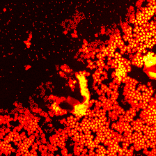
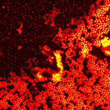
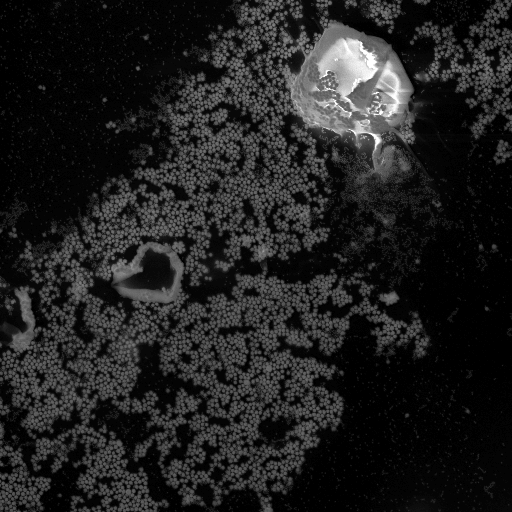
The object used to simulate the diffraction pattern is obtained from an SEM image of a cluster of commercial 50 nm colloidal gold spheres. The image is shown in Fig. 3. The gray scale values were converted to a sample thickness varying between 0 and 50 nm, and we assigned the complex index of refraction of a 750 eV x ray photon going through an organic compound (PMMA). Here the numerical tests are done assuming periodic boundary conditions. These boundary conditions ensure that every region of the object ψ𝜓\psi is illuminated with an equal number of overlapping frames, in other words the null space of Q𝑄Q is empty. We use frame width 16×16161616\times 16, probe width 888, step size 555, number of frames 8×864×648864648\times 8\ldots 64\times 64, RAAR algorithm, β=.75𝛽.75\beta=.75. The initial guess of the phase chosen to be random. There is no padding of the illumination function shown in Fig. 3 (the intensity measurement is slightly under-sampled).

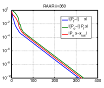
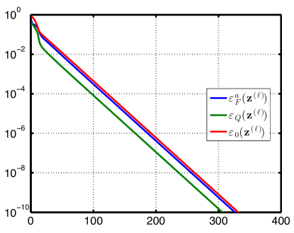
The metrics εF,εqsubscript𝜀𝐹subscript𝜀𝑞\varepsilon_{F},\varepsilon_{q} used to monitor progress are functions depending on 𝒛()superscript𝒛{\bm{z}}^{(\ell)}:

εF(𝒛())subscript𝜀𝐹superscript𝒛\displaystyle\varepsilon_{F}\left({\bm{z}}^{(\ell)}\right) =\displaystyle= [PFI]𝒛()𝒂,normdelimited-[]subscript𝑃𝐹𝐼superscript𝒛norm𝒂\displaystyle\tfrac{\left\|\left[P_{F}-I\right]{\bm{z}}^{(\ell)}\right\|}{\|\bm{a}\|},
εQ(𝒛())subscript𝜀𝑄superscript𝒛\displaystyle\varepsilon_{Q}\left({\bm{z}}^{(\ell)}\right) =\displaystyle= [PQI]𝒛()𝒂normdelimited-[]subscript𝑃𝑄𝐼superscript𝒛norm𝒂\displaystyle\tfrac{\left\|\left[P_{Q}-I\right]{\bm{z}}^{(\ell)}\right\|}{\|\bm{a}\|}

where I𝐼I is the identity operator. This has to be compared to ε0subscript𝜀0\varepsilon_{0}, the error w.r.t the known solution:

ε0(𝒛())subscript𝜀0superscript𝒛\displaystyle\varepsilon_{0}\left({\bm{z}}^{(\ell)}\right) =\displaystyle= 1𝒂minφeiφ𝒛()𝑸ψ,1norm𝒂subscript𝜑normsuperscript𝑒𝑖𝜑superscript𝒛𝑸𝜓\displaystyle\tfrac{1}{\|\bm{a}\|}{\min_{\varphi}\left\|e^{i\varphi}{\bm{z}}^{(\ell)}-{\bm{Q}}\psi\right\|},

where φ𝜑\varphi is an arbitrary global phase factor.

We report the following observations

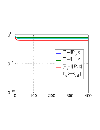
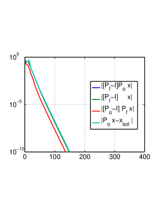
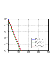
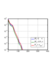
  • Fluctuating intensities: (Fig. 4) The intensity fluctuation in this tests are 20%percent2020\%. By solving the new LSQ problem introduced in (35), we obtain accelerated convergence and exact reconstructions every time we tested the problem, see (Fig. 4). No degradation (above numerical precision) introduced by intensities perturbed by 20%percent2020\%.

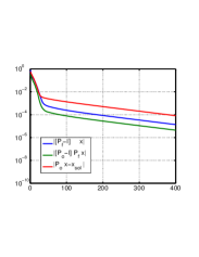
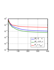
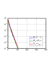
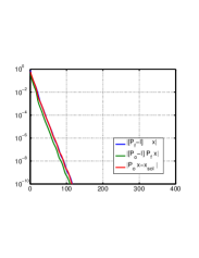
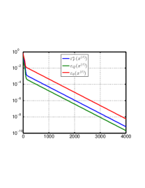
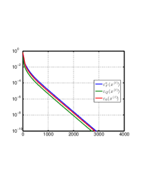
  • Scaling: (Fig. 5) We show improved convergence in the larger scale problems. The results are summarized in Table 3. As we increase the number of frames, convergence slows down for standard projection operators. The parameters used in this simulation are m=16𝑚16m=16, Dx=4subscript𝐷𝑥4D_{x}=4, k𝑘k varies and n=kDx+m𝑛𝑘subscript𝐷𝑥𝑚n=kD_{x}+m, where Dxsubscript𝐷𝑥D_{x} is the step size of the illumination windows.

  • Incoherent Multiplexing: (Fig. 5) Deconvolution of the incoherent sum of frames translated by 3 times the illuminating beam width.

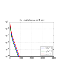
  • Incoherent beams with fluctuations: (Fig. 6). Deconvolution of the incoherent sum of frames translated by 3 times the illuminating beam width, with unknown amplitude.

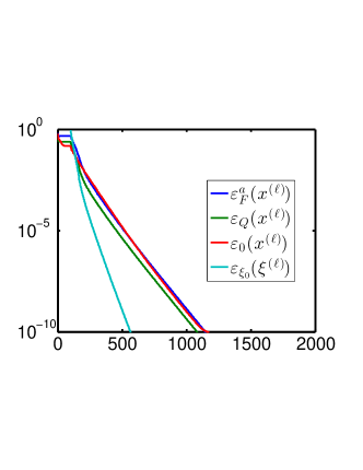
  • Positions: (Fig. 7) Recovery of the positions perturbed by an unknown factor randomly distributed between ±2.5plus-or-minus2.5\pm 2.5 pixels.

  • Background: (Fig. 8, Fig. 9) 𝒛(i)i/b=0.5subscriptdelimited-⟨⟩normsubscript𝒛𝑖𝑖norm𝑏0.5\langle\|{\bm{z}}_{(i)}\|\rangle_{i}/\|b\|=0.5. In Figure 8,9 we obtain exact reconstruction of the object and background (Background ratio a/b=106norm𝑎norm𝑏superscript106\|a\|/\|b\|=10^{-6}). Exact recovery (within numerical precision) was obtained with step size δx=3r𝛿𝑥3𝑟\delta x=3r. No degradation (above numerical precision) introduced by the background, nearly no influence on convergence rate.

  • Missing data: (Fig. 12, Fig. 12) Exact recovery (within numerical precision) using Eq (29). Frame size:32x32, number of frames: 16x16, step size:3.5 pixels.

# frames clock time(s) iteration ε02superscriptsubscript𝜀02\varepsilon_{0}^{2}
standard
4×\times4 0.7 121 <<1e-11
8×\times8 1.4 125 <<1e-11
16×\times16 4.9 144 <<1e-11
24×\times24 26.3 400 4.3e-10
32×\times32 36.3 400 4.3e-4
48×\times48 90.7 400 3.4e-4
64×\times64 137.5 400 5.3e-3
augmented
4×\times4 1.9 138 <<1e-11
8×\times8 2.7 141 <<1e-11
16×\times16 6.5 138 <<1e-11
24×\times24 14 134 <<1e-11
32×\times32 25.6 139 <<1e-11
48×\times48 60.4 142 <<1e-11
64×\times64 96.2 149 <<1e-11
Table 3: Performance of projection algorithms using matlab R2012a 64-bit (maci64) (lapack version 3.3.1, MKL 10.3.5) on 2x2.2GHz Quad-core Intel xeon using frames of dimension 16×16161616\times 16 .

Conclusions

While phase retrieval problems are notoriously difficult to solve numerically, the high redundancy in ptychographic data enables not only robust phase recoveryThibault-Guizar ; Godard:12 but the recovery of other parameters such as the illuminating function itselfthibault:probe , position Maiden:2012 ; fienup ; axel , coherence function clark:2011 , etc.

In this paper we introduce a modified projection operator for the ptychographic reconstruction problem that accounts for fluctuating intensities, position errors, partial coherence or poor calibration using multiplexing illumination, and an unknown offset (background) difference for every pixel but constant throughout the acquisition (or vice versa). Our approach starts from the redundant measurement space and computes pairwise comparison between frames before merging into the object space. We describe first order methods to minimize the gap between measurement space and object space w.r.t. the perturbation parameter. We show that our method enhances the convergence rate of common projection algorithms. We show several cases where missing information (phases, bad pixels, positions, incoherence, etc.) was retrieved exactly (to within numerical precision) starting from random phases. This method appears to be robust when the amount of overlap between neighboring frames is around 50% or more.

Further theoretical analysis on the relative merits between object-space minimization and measurement space minimization will be the subject of the future work.

Here some numerical details deserve further developments. By optimizing the phase of each frame from the redundant measurement space, we solve the phase problem at a resolution given by the step size between frames. This intra-frame phase optimization may be applied to merge subregions reconstructed independently by distributed computer systems. For three dimensional objects, we could apply similar approach to merge two dimensional views reconstructed independently into one three dimensional object. Finally, this intra-frame optimization could be applied to multi-scale reconstructions where frames are divided in regions of Fourier space, or it could be applied to correct low order phase aberrations between frames. More work is needed to to establish the optimal frequency of communication and the amount of overlap between sub-reconstruction regions.

Acknowledgments

The authors thank Prof. Bin Yu and Jeff Donatelli for discussions. This research was supported in part by the Applied Mathematical Sciences subprogram of the Office of Energy Research, U.S. Department of Energy, under contract DE-AC02-05CH11231 (SM,CY), and by the Laboratory Directed Research and Development Program of Lawrence Berkeley National Laboratory under the U.S. Department of Energy contract number DE-AC02-05CH11231 (A. S.), and by the Director, Office of Science, Advanced Scientific Computing Research, of the U.S. Department of Energy under Contract No. DE-AC02-05CH11231 (F.M.). The computational results presented were obtained at the National Energy Research Scientific Computing Center (NERSC), which is supported by the Director, Office of Advanced Scientific Computing Research of the U.S. Department of Energy under contract number DE-AC02-05CH11232. Hau-tieng Wu acknowledges the support by Purdue National Science Foundation of United States (CCF-0939370) and Focused Research Group (DMS-1160319).

Appendix A Intensity fluctuations

One of the practical issues one may face in ptychography is the intensity fluctuation among different diffraction frames introduced by instabilities in the light source, optics and shutters. Such fluctuation can be accounted for by introducing a scaling factor ωisubscript𝜔𝑖\omega_{i}\in\mathbb{C} for each diffraction frame, As a result, the definition z^isubscript^𝑧𝑖\hat{z}_{i} is modified so that the equation

ωiz(i)=Q(i)ψ,subscript𝜔𝑖subscript𝑧𝑖subscript𝑄𝑖𝜓\omega_{i}z_{(i)}=Q_{(i)}\psi, (51)

holds for i=1,2,,k𝑖12𝑘i=1,2,...,k.

Since both ωisubscript𝜔𝑖\omega_{i} and ψ𝜓\psi are unknown in (51), the solution to (51) is clearly not unique. To exclude the trivial solution ωi=0subscript𝜔𝑖0\omega_{i}=0, for i=1,2,k𝑖12𝑘i=1,2,...k and ψ=0𝜓0\psi=0, we introduce an additional constraint and solve

(ψmin,ω(i))=argminψ,ω(i)iQ(i)ψωiz(i)2subscript𝜓subscript𝜔𝑖subscript𝜓subscript𝜔𝑖subscript𝑖superscriptnormsubscript𝑄𝑖𝜓subscript𝜔𝑖subscript𝑧𝑖2\displaystyle\left(\psi_{\min},\omega_{(i)}\right)=\arg\min_{\psi,\omega_{(i)}}\sum_{i}\left\|Q_{(i)}\psi-\omega_{i}z_{(i)}\right\|^{2} (52)
subject to (i)ωi=(i)1=k,subject to (i)ωi=(i)1=k\displaystyle\text{ subject to $\sum_{(i)}\omega_{i}=\sum_{(i)}1=k$},

which is equivalent to solve

minψ,ωi,λ(ψ,ωi,λ),where =iQ(i)ψωiz(i)2+2λ(iωi𝟏2),subscript𝜓subscript𝜔𝑖𝜆𝜓subscript𝜔𝑖𝜆where subscript𝑖superscriptnormsubscript𝑄𝑖𝜓subscript𝜔𝑖subscript𝑧𝑖22𝜆subscript𝑖subscript𝜔𝑖superscriptnorm12\min_{\psi,\omega_{i},\lambda}{\cal L}(\psi,\omega_{i},\lambda),\,\text{where }\,{\cal L}=\sum_{i}\|Q_{(i)}\psi-\omega_{i}z_{(i)}\|^{2}+2\lambda\left(\sum_{i}\omega_{i}-\|\bm{1}\|^{2}\right), (53)

where λ𝜆\lambda is a Lagrange multiplier. To find the coefficients ωisubscript𝜔𝑖\omega_{i}, we use the normal equation associated with the LSQ problem (Eq. 53) :

(iQ(i)Q(i)Q1z1Qkzk0z1Q1z1z100100zkQk00zkzk10110)(ψω1ωkλ)=(000𝟏2).subscript𝑖superscriptsubscript𝑄𝑖subscript𝑄𝑖superscriptsubscript𝑄1subscript𝑧1superscriptsubscript𝑄𝑘subscript𝑧𝑘0superscriptsubscript𝑧1subscript𝑄1superscriptsubscript𝑧1subscript𝑧10010missing-subexpressionmissing-subexpressionmissing-subexpression0missing-subexpressionsuperscriptsubscript𝑧𝑘subscript𝑄𝑘00superscriptsubscript𝑧𝑘subscript𝑧𝑘101missing-subexpression10𝜓subscript𝜔1subscript𝜔𝑘𝜆000superscriptnorm12\left(\begin{array}[]{cccccc}\sum_{i}Q_{(i)}^{\ast}Q_{(i)}&-Q_{1}^{\ast}z_{1}&\ldots&\ldots&-Q_{k}^{\ast}z_{k}&0\\ -z_{1}^{\ast}Q_{1}&z_{1}^{\ast}z_{1}&0&\ldots&0&1\\ \vdots&0&\ddots&&\vdots&\vdots\\ \vdots&\vdots&&&0&\\ -z_{k}^{\ast}Q_{k}&0&\ldots&0&z_{k}^{\ast}z_{k}&1\\ 0&1&\ldots&&1&0\end{array}\right)\left(\begin{array}[]{c}\psi\\ \omega_{1}\\ \vdots\\ \omega_{k}\\ \lambda\end{array}\right)=\left(\begin{array}[]{c}0\\ 0\\ \vdots\\ 0\\ \|\bm{1}\|^{2}\end{array}\right).

We can partition the equation above as

(AB𝟎BD𝟏𝟎𝟏𝟎)(ψ𝝎λ)=(00𝟏2),𝐴superscript𝐵0𝐵𝐷10superscript10𝜓𝝎𝜆00superscriptnorm12\left(\begin{array}[]{ccc}A&B^{\ast}&\bm{0}\\ B&D&\bm{1}\\ \bm{0}&\bm{1}^{\ast}&\bm{0}\end{array}\right)\left(\begin{array}[]{c}\psi\\ {\bm{\omega}}\\ \lambda\end{array}\right)=\left(\begin{array}[]{c}0\\ 0\\ \|\bm{1}\|^{2}\\ \end{array}\right),\,

where

A=i=1kQ(i)Q(i),B=(z1Q1zkQk),D=(z1z1000z2z2000zkzk),𝝎=(ω1ωk).formulae-sequence𝐴superscriptsubscript𝑖1𝑘superscriptsubscript𝑄𝑖subscript𝑄𝑖formulae-sequence𝐵superscriptsubscript𝑧1subscript𝑄1superscriptsubscript𝑧𝑘subscript𝑄𝑘formulae-sequence𝐷superscriptsubscript𝑧1subscript𝑧100missing-subexpression0superscriptsubscript𝑧2subscript𝑧2missing-subexpression0missing-subexpression00superscriptsubscript𝑧𝑘subscript𝑧𝑘missing-subexpression𝝎subscript𝜔1subscript𝜔𝑘A=\sum_{i=1}^{k}Q_{(i)}^{\ast}Q_{(i)},\ \ B=\left(\begin{array}[]{c}-z_{1}^{\ast}Q_{1}\\ \vdots\\ -z_{k}^{\ast}Q_{k}\end{array}\right),\ \ D=\left(\begin{array}[]{ccccc}z_{1}^{\ast}z_{1}&0&\ldots&0\\ 0&z_{2}^{\ast}z_{2}&\ddots&\vdots\\ \vdots&\ddots&\ddots&0\\ 0&\ldots&0&z_{k}^{\ast}z_{k}\\ \end{array}\right),\quad\bm{\omega}=\left(\begin{array}[]{c}\omega_{1}\\ \vdots\\ \omega_{k}\end{array}\right).

By the block factorization

(I00BA1I00𝟏H11)(AB𝟎𝟎H𝟏𝟎𝟎𝟏H1𝟏)(ψ𝝎λ)=(00𝟏2),𝐼00𝐵superscript𝐴1𝐼00superscript1superscript𝐻11𝐴superscript𝐵00𝐻100superscript1superscript𝐻11𝜓𝝎𝜆00superscriptnorm12\displaystyle\left(\begin{array}[]{ccc}I&0&0\\ -BA^{-1}&I&0\\ 0&-\bm{1}^{\ast}H^{-1}&1\\ \end{array}\right)\left(\begin{array}[]{ccc}A&B^{\ast}&\bm{0}\\ \bm{0}&H&\bm{1}\\ \bm{0}&\bm{0}&-\bm{1}^{\ast}H^{-1}\bm{1}\\ \end{array}\right)\left(\begin{array}[]{c}\psi\\ {\bm{\omega}}\\ \lambda\end{array}\right)=\left(\begin{array}[]{c}0\\ 0\\ \|\bm{1}\|^{2}\\ \end{array}\right), (66)

where the Schur complement H=DBA1B𝐻𝐷𝐵superscript𝐴1superscript𝐵H=D-BA^{-1}B^{\ast} is given by

Hi,j=z(i)(δi,jIQ(i)((ι)Q(ι)Q(ι))1Q(j))z(j).subscript𝐻𝑖𝑗superscriptsubscript𝑧𝑖subscript𝛿𝑖𝑗𝐼subscript𝑄𝑖superscriptsubscript𝜄superscriptsubscript𝑄𝜄subscript𝑄𝜄1superscriptsubscript𝑄𝑗subscript𝑧𝑗H_{i,j}=z_{(i)}^{\ast}\left(\delta_{i,j}I-Q_{(i)}\left(\sum_{(\iota)}Q_{(\iota)}^{\ast}Q_{(\iota)}\right)^{-1}Q_{(j)}^{\ast}\right)z_{(j)}.

By block-wise inversion of Eq. 66, we obtain 𝝎𝝎\bm{\omega} and the scaling factor λ𝜆\lambda from a sparse linear equation:

H𝝎=λ𝟏,λ=𝟏2𝟏H1𝟏.formulae-sequence𝐻𝝎𝜆1𝜆superscriptnorm12superscript1superscript𝐻11H\bm{\omega}=-\lambda\bm{1},\qquad\lambda=-\tfrac{\|\bm{1}\|^{2}}{\bm{1}^{\ast}H^{-1}\bm{1}}\,.

Eigenvalue method

If we make a change of variable, ν(i)=z(i)ω(i)subscript𝜈𝑖normsubscript𝑧𝑖subscript𝜔𝑖\nu_{(i)}=\|z_{(i)}\|\omega_{(i)}, we can re-write the problem argmin𝝎𝝎H𝝎subscript𝝎superscript𝝎𝐻𝝎\arg\min_{\bm{\omega}}\bm{\omega}^{\ast}H\bm{\omega} as:

argmin𝝂subscript𝝂\displaystyle\arg\min_{\bm{\nu}} 𝝂2𝝂K𝝂,Ki,j=z(i)z(i)Q(i)((ι)Q(ι)Q(ι))1Q(j)z(j)z(j).superscriptnorm𝝂2superscript𝝂𝐾𝝂subscript𝐾𝑖𝑗superscriptsubscript𝑧𝑖normsubscript𝑧𝑖subscript𝑄𝑖superscriptsubscript𝜄superscriptsubscript𝑄𝜄subscript𝑄𝜄1superscriptsubscript𝑄𝑗subscript𝑧𝑗normsubscript𝑧𝑗\displaystyle\quad\|\bm{\nu}\|^{2}-\bm{\nu}^{\ast}K\bm{\nu},\qquad K_{i,j}=\frac{z_{(i)}^{\ast}}{\|z_{(i)}\|}Q_{(i)}\left(\sum_{(\iota)}Q_{(\iota)}^{\ast}Q_{(\iota)}\right)^{-1}Q_{(j)}^{\ast}\frac{z_{(j)}}{\|z_{(j)}\|}.

The solution to this problem assuming νnorm𝜈\|\nu\|=constant is the eigenvector corresponding to the largest eigenvalue of the sparse matrix K𝐾K. This can be computed efficiently using packages such asarpack

Appendix B Taylor expansion

We consider the case in which the probe w𝑤w is translated from the input coordinate by an unknown distance ξ𝜉\xi. We restrict ourselves to the 111-dim ptychography problem to simplify the discussion. We call 𝑸ξsubscript𝑸𝜉{\bm{Q}}_{\xi} the unknown illumination matrix used to generate the data. To determine the illumination matrix, we determine the parameter ξ𝜉\xi so that the error ε𝑸ξsubscript𝜀subscript𝑸𝜉\varepsilon_{{\bm{Q}}_{\xi}} is minimized:

argminξksubscript𝜉superscript𝑘\displaystyle\arg\min_{\xi\in\mathbb{R}^{k}} [IP𝑸ξ]𝒛2superscriptnormdelimited-[]𝐼subscript𝑃subscript𝑸𝜉𝒛2\displaystyle\left\|\left[I-P_{{\bm{Q}}_{\xi}}\right]{\bm{z}}\right\|^{2} , (67)

where the i𝑖i-th entry of ξk𝜉superscript𝑘\xi\in\mathbb{R}^{k} represents the translation distance of the i𝑖i-th frame. Given the illumination function w𝑤w, we can compute the first and second order derivatives with respect to translation. We denote by Qi,Ri,Sisubscript𝑄𝑖subscript𝑅𝑖subscript𝑆𝑖Q_{i},R_{i},S_{i} the illumination matrices that extract a frame out of an image and multiplies by (w(𝒙),xw(𝒙)𝑤𝒙subscript𝑥𝑤𝒙w({\bm{x}}),\partial_{x}w({\bm{x}}), x2w(𝒙)superscriptsubscript𝑥2𝑤𝒙\partial_{x}^{2}w({\bm{x}})) respectively. Build 𝑸,𝑹,𝑺𝑸𝑹𝑺{\bm{Q}},{\bm{R}},{\bm{S}} from Qi,Ri,Sisubscript𝑄𝑖subscript𝑅𝑖subscript𝑆𝑖Q_{i},R_{i},S_{i}, which are tall and skinny matrices of the same size as 𝑸𝑸{\bm{Q}} discussed earlier, with identical location of the non-zero entries. Assume that the probe is perturbed to second order as follows:

𝑸ξ=𝑸+ξ𝑹+ξ2𝑺.subscript𝑸𝜉𝑸𝜉𝑹superscript𝜉2𝑺{\bm{Q}}_{\xi}={\bm{Q}}+\xi{\bm{R}}+\xi^{2}{\bm{S}}.

where, by a slight abuse of notation, ξ𝜉\xi denotes a diagonal and real matrix so that the i𝑖i-th diagonal entry, denoted as ξisubscript𝜉𝑖\xi_{i} represents the translation distance of the i𝑖i-th frame. With 𝑸ξsubscript𝑸𝜉{\bm{Q}}_{\xi} plugged into (67), we now minimize

argminξksubscript𝜉superscript𝑘\displaystyle\arg\min_{\xi\in\mathbb{R}^{k}} [I(𝑸+ξ𝑹+ξ2𝑺)[(𝑸+ξ𝑹+ξ2𝑺)(𝑸+ξ𝑹+ξ2𝑺)]1(𝑸+ξ𝑹+ξ2𝑺)]𝒛2.superscriptnormdelimited-[]𝐼𝑸𝜉𝑹superscript𝜉2𝑺superscriptdelimited-[]superscript𝑸𝜉𝑹superscript𝜉2𝑺𝑸𝜉𝑹superscript𝜉2𝑺1superscript𝑸𝜉𝑹superscript𝜉2𝑺𝒛2\displaystyle\small{\left\|\left[I-\left({\bm{Q}}+\xi{\bm{R}}+{\xi^{2}}{\bm{S}}\right)\left[\left({\bm{Q}}+\xi{\bm{R}}+{\xi^{2}}{\bm{S}}\right)^{\ast}\left({\bm{Q}}+\xi{\bm{R}}+{\xi^{2}}{\bm{S}}\right)\right]^{-1}\left({\bm{Q}}+\xi{\bm{R}}+{\xi^{2}}{\bm{S}}\right)^{\ast}\right]{\bm{z}}\right\|^{2}.} (68)

By Taylor expansion:

[]11𝑸𝑸(1(𝑹ξ𝑸+𝑸ξ𝑹+O(ξ2))1𝑸𝑸),similar-to-or-equalssuperscriptdelimited-[]11superscript𝑸𝑸1superscript𝑹𝜉𝑸superscript𝑸𝜉𝑹𝑂superscript𝜉21superscript𝑸𝑸[\cdot]^{-1}\simeq\frac{1}{{\bm{Q}}^{\ast}{\bm{Q}}}\left(1-({\bm{R}}^{\ast}\xi{\bm{Q}}+{\bm{Q}}^{\ast}\xi{\bm{R}}+O(\xi^{2}))\frac{1}{{\bm{Q}}^{\ast}{\bm{Q}}}\right),

when 𝑸𝑸superscript𝑸𝑸{\bm{Q}}^{\ast}{\bm{Q}} is invertible. The second order term O(ξ2)𝑂superscript𝜉2O(\xi^{2}) includes other second order terms that we will not need. We write the expansion of the residual in Eq. (68) f0+f1(ξ)+f2(ξ2)subscript𝑓0subscript𝑓1𝜉subscript𝑓2superscript𝜉2f_{0}+f_{1}(\xi)+f_{2}(\xi^{2}) as:

f0subscript𝑓0\displaystyle f_{0} =\displaystyle= [IP𝑸]𝒛𝒛¯delimited-[]𝐼subscript𝑃𝑸𝒛¯𝒛\displaystyle[I-P_{\bm{Q}}]{\bm{z}}\equiv\underline{\bm{z}} (69)

We define ϕ1𝑸𝑸𝑸superscriptitalic-ϕ1superscript𝑸𝑸superscript𝑸\phi^{\ast}\equiv\frac{1}{{\bm{Q}}^{\ast}{\bm{Q}}}{\bm{Q}}^{\ast}, and express the first order as

f1(ξ)subscript𝑓1𝜉\displaystyle f_{1}(\xi) =\displaystyle= [ξ𝑹ϕϕ𝑹ξ+ϕ(𝑹ξ𝑸+𝑸ξ𝑹)ϕ]𝒛.delimited-[]𝜉𝑹superscriptitalic-ϕitalic-ϕsuperscript𝑹𝜉italic-ϕsuperscript𝑹𝜉𝑸superscript𝑸𝜉𝑹superscriptitalic-ϕ𝒛\displaystyle\left[-\xi{\bm{R}}\phi^{\ast}-\phi{\bm{R}}^{\ast}\xi+\phi({\bm{R}}^{\ast}\xi{\bm{Q}}+{\bm{Q}}^{\ast}\xi{\bm{R}})\phi^{\ast}\right]{\bm{z}}.

By defining 𝒛𝑹𝑹ϕ𝒛subscript𝒛𝑹𝑹superscriptitalic-ϕ𝒛{\bm{z}}_{\bm{R}}\equiv{\bm{R}}\phi^{\ast}{\bm{z}}, using P𝑸=𝑸ϕ=ϕ𝑸subscript𝑃𝑸𝑸superscriptitalic-ϕitalic-ϕsuperscript𝑸P_{\bm{Q}}={\bm{Q}}\phi^{\ast}=\phi{\bm{Q}}^{\ast}, and rearranging, we get

f1(ξ)subscript𝑓1𝜉\displaystyle f_{1}(\xi) =\displaystyle= ξ𝒛𝑹ϕ𝑹ξ(𝒛𝑸ϕ𝒛)+ϕ𝑸ξ𝒛𝑹𝜉subscript𝒛𝑹italic-ϕsuperscript𝑹𝜉𝒛𝑸superscriptitalic-ϕ𝒛italic-ϕsuperscript𝑸𝜉subscript𝒛𝑹\displaystyle-\xi{\bm{z}}_{\bm{R}}-\phi{\bm{R}}^{\ast}\xi({\bm{z}}-{\bm{Q}}\phi^{\ast}{\bm{z}})+\phi{\bm{Q}}^{\ast}\xi{\bm{z}}_{\bm{R}} (70)
=\displaystyle= (1P𝑸)ξ𝒛𝑹ϕ𝑹ξ𝒛¯.1subscript𝑃𝑸𝜉subscript𝒛𝑹italic-ϕsuperscript𝑹𝜉¯𝒛\displaystyle-(1-P_{\bm{Q}})\xi{\bm{z}}_{\bm{R}}-\phi{\bm{R}}^{\ast}\xi\underline{\bm{z}}.

By using the equality 𝒛¯(IPQ)=𝒛¯¯𝒛𝐼subscript𝑃𝑄¯𝒛\underline{\bm{z}}(I-P_{Q})=\underline{\bm{z}}, setting O𝑹𝑹ϕϕ𝑹=𝑹1𝑸𝑸𝑹subscript𝑂𝑹𝑹superscriptitalic-ϕitalic-ϕsuperscript𝑹𝑹1superscript𝑸𝑸superscript𝑹O_{\bm{R}}\equiv{\bm{R}}\phi^{\ast}\phi{\bm{R}}^{\ast}={\bm{R}}\frac{1}{{\bm{Q}}^{\ast}{\bm{Q}}}{\bm{R}}^{\ast} and rearranging, we obtain:

f2(ξ)subscript𝑓2𝜉\displaystyle f_{2}(\xi) =\displaystyle= [ξ𝑹1𝑸𝑸𝑹ξ+ξ2𝑺ϕ+𝑸O(ξ2)]𝒛delimited-[]𝜉𝑹1superscript𝑸𝑸superscript𝑹𝜉superscript𝜉2𝑺italic-ϕ𝑸𝑂superscript𝜉2𝒛\displaystyle-\left[\xi{\bm{R}}\tfrac{1}{{\bm{Q}}^{\ast}{\bm{Q}}}{\bm{R}}^{\ast}\xi+{\xi^{2}}{\bm{S}}\phi+{\bm{Q}}O\left(\xi^{2}\right)\right]{\bm{z}} (71)
=\displaystyle= ξO𝑹ξ𝒛ξ2𝒛𝑺+𝑸O(ξ2)𝒛𝜉subscript𝑂𝑹𝜉𝒛superscript𝜉2subscript𝒛𝑺𝑸𝑂superscript𝜉2𝒛\displaystyle-\xi O_{\bm{R}}\xi{\bm{z}}-{\xi^{2}}{\bm{z}}_{\bm{S}}+{\bm{Q}}O\left(\xi^{2}\right){\bm{z}}

where 𝒛𝑺𝑺ϕ𝒛subscript𝒛𝑺𝑺superscriptitalic-ϕ𝒛{\bm{z}}_{\bm{S}}\equiv{\bm{S}}\phi^{\ast}{\bm{z}}. We rewrite Eq. (68) above as:

[IPQξ]𝒛2=f0f0+f0f1+f1f0+f1f1+f0f2+f2f0+O(ξ3).superscriptnormdelimited-[]𝐼subscript𝑃subscript𝑄𝜉𝒛2superscriptsubscript𝑓0subscript𝑓0superscriptsubscript𝑓0subscript𝑓1superscriptsubscript𝑓1subscript𝑓0superscriptsubscript𝑓1subscript𝑓1superscriptsubscript𝑓0subscript𝑓2superscriptsubscript𝑓2subscript𝑓0𝑂superscript𝜉3\left\|\left[I-P_{Q_{\xi}}\right]{\bm{z}}\right\|^{2}=f_{0}^{\ast}f_{0}+f_{0}^{\ast}f_{1}+f_{1}^{\ast}f_{0}+f_{1}^{\ast}f_{1}+f_{0}^{\ast}f_{2}+f_{2}^{\ast}f_{0}+O(\xi^{3}).

Note that 𝒛¯𝑸=𝒛¯ϕ=0superscript¯𝒛𝑸superscript¯𝒛italic-ϕ0\underline{\bm{z}}^{\ast}{\bm{Q}}=\underline{\bm{z}}^{\ast}\phi=0. Set 𝒛𝑸𝑸ϕ𝒛subscript𝒛𝑸𝑸italic-ϕ𝒛{\bm{z}}_{\bm{Q}}\equiv{\bm{Q}}\phi{\bm{z}} and obtain the first and second order terms of Eq. (68):

f0f1+f1f0superscriptsubscript𝑓0subscript𝑓1superscriptsubscript𝑓1subscript𝑓0\displaystyle f_{0}^{\ast}f_{1}+f_{1}^{\ast}f_{0} =\displaystyle= 𝒛¯ξ𝒛𝑹,𝒛𝑹ξ𝒛¯superscript¯𝒛𝜉subscript𝒛𝑹superscriptsubscript𝒛𝑹𝜉¯𝒛\displaystyle-\underline{\bm{z}}^{\ast}\xi{\bm{z}}_{\bm{R}},-{\bm{z}}_{\bm{R}}^{\ast}\xi\underline{\bm{z}} (72)
f1f1+f0f2+f2f0superscriptsubscript𝑓1subscript𝑓1superscriptsubscript𝑓0subscript𝑓2superscriptsubscript𝑓2subscript𝑓0\displaystyle f_{1}^{\ast}f_{1}+f_{0}^{\ast}f_{2}+f_{2}^{\ast}f_{0} =\displaystyle= 𝒛𝑹ξ(IP𝑸)ξ𝒛𝑹+𝒛¯ξO𝑹ξ𝒛¯𝒛¯ξO𝑹ξ𝒛𝒛¯ξ2𝒛𝑺𝒛ξO𝑹ξ𝒛¯𝒛𝑺ξ2𝒛¯,subscriptsuperscript𝒛𝑹𝜉𝐼subscript𝑃𝑸𝜉subscript𝒛𝑹¯𝒛𝜉subscript𝑂𝑹𝜉¯𝒛superscript¯𝒛𝜉subscript𝑂𝑹𝜉𝒛superscript¯𝒛superscript𝜉2subscript𝒛𝑺superscript𝒛𝜉subscript𝑂𝑹𝜉¯𝒛superscriptsubscript𝒛𝑺superscript𝜉2¯𝒛\displaystyle{\bm{z}}^{\ast}_{\bm{R}}\xi(I-P_{\bm{Q}})\xi{\bm{z}}_{\bm{R}}+\underline{\bm{z}}\xi O_{\bm{R}}\xi\underline{\bm{z}}-\underline{\bm{z}}^{\ast}\xi O_{\bm{R}}\xi{\bm{z}}-\underline{\bm{z}}^{\ast}{\xi^{2}}{\bm{z}}_{\bm{S}}-{\bm{z}}^{\ast}\xi O_{\bm{R}}\xi\underline{\bm{z}}-{\bm{z}}_{\bm{S}}^{\ast}{\xi^{2}}\underline{\bm{z}},
=\displaystyle= 𝒛𝑹ξ2𝒛𝑹𝒛¯ξ2𝒛𝑺𝒛𝑺ξ2𝒛¯𝒛ξO𝑹ξ𝒛+𝒛𝑸ξO𝑹ξ𝒛𝑸𝒛𝑹ξP𝑸ξ𝒛𝑹,subscriptsuperscript𝒛𝑹superscript𝜉2subscript𝒛𝑹superscript¯𝒛superscript𝜉2subscript𝒛𝑺superscriptsubscript𝒛𝑺superscript𝜉2¯𝒛superscript𝒛𝜉subscript𝑂𝑹𝜉𝒛superscriptsubscript𝒛𝑸𝜉subscript𝑂𝑹𝜉subscript𝒛𝑸subscriptsuperscript𝒛𝑹𝜉subscript𝑃𝑸𝜉subscript𝒛𝑹\displaystyle{\bm{z}}^{\ast}_{\bm{R}}\xi^{2}{\bm{z}}_{\bm{R}}-\underline{\bm{z}}^{\ast}{\xi^{2}}{\bm{z}}_{\bm{S}}-{\bm{z}}_{\bm{S}}^{\ast}{\xi^{2}}\underline{\bm{z}}-{\bm{z}}^{\ast}\xi O_{\bm{R}}\xi{\bm{z}}+{\bm{z}}_{{\bm{Q}}}^{\ast}\xi O_{\bm{R}}\xi{\bm{z}}_{{\bm{Q}}}-{\bm{z}}^{\ast}_{\bm{R}}\xi P_{\bm{Q}}\xi{\bm{z}}_{\bm{R}},

By using the definition of 𝒛𝑸subscript𝒛𝑸{\bm{z}}_{\bm{Q}}, 𝒛𝑹subscript𝒛𝑹{\bm{z}}_{\bm{R}}, P𝑸subscript𝑃𝑸P_{\bm{Q}} and O𝑹subscript𝑂𝑹O_{\bm{R}} it is easy to show that 𝒛𝑸ξO𝑹ξ𝒛𝑸=𝒛𝑹ξP𝑸ξ𝒛𝑹superscriptsubscript𝒛𝑸𝜉subscript𝑂𝑹𝜉subscript𝒛𝑸subscriptsuperscript𝒛𝑹𝜉subscript𝑃𝑸𝜉subscript𝒛𝑹{\bm{z}}_{{\bm{Q}}}^{\ast}\xi O_{\bm{R}}\xi{\bm{z}}_{{\bm{Q}}}={\bm{z}}^{\ast}_{\bm{R}}\xi P_{\bm{Q}}\xi{\bm{z}}_{\bm{R}} and simplify as:

f1f1+f0f2+f2f0superscriptsubscript𝑓1subscript𝑓1superscriptsubscript𝑓0subscript𝑓2superscriptsubscript𝑓2subscript𝑓0\displaystyle f_{1}^{\ast}f_{1}+f_{0}^{\ast}f_{2}+f_{2}^{\ast}f_{0} =\displaystyle= 𝒛𝑹ξ2𝒛𝑹𝒛¯ξ2𝒛𝑺𝒛𝑺ξ2𝒛¯𝒛ξO𝑹ξ𝒛.subscriptsuperscript𝒛𝑹superscript𝜉2subscript𝒛𝑹superscript¯𝒛superscript𝜉2subscript𝒛𝑺superscriptsubscript𝒛𝑺superscript𝜉2¯𝒛superscript𝒛𝜉subscript𝑂𝑹𝜉𝒛\displaystyle{\bm{z}}^{\ast}_{\bm{R}}\xi^{2}{\bm{z}}_{\bm{R}}-\underline{\bm{z}}^{\ast}{\xi^{2}}{\bm{z}}_{\bm{S}}-{\bm{z}}_{\bm{S}}^{\ast}{\xi^{2}}\underline{\bm{z}}-{\bm{z}}^{\ast}\xi O_{\bm{R}}\xi{\bm{z}}. (73)

By setting ξi2=0\partial_{\xi_{i}}\|\cdot\|^{2}=0 in Eq. (68), we obtain the linear equation for solving ξ𝜉\xi:

j(2(𝒛𝑹i𝒛𝑹i𝒛¯i𝒛𝑺i𝒛𝑺i𝒛¯i)δij𝒛iO𝑹ij𝒛j𝒛jO𝑹ji𝒛i)ξjsubscript𝑗2superscriptsubscript𝒛subscript𝑹𝑖subscript𝒛subscript𝑹𝑖superscriptsubscript¯𝒛𝑖subscript𝒛subscript𝑺𝑖superscriptsubscript𝒛subscript𝑺𝑖subscript¯𝒛𝑖subscript𝛿𝑖𝑗superscriptsubscript𝒛𝑖subscript𝑂subscript𝑹𝑖𝑗subscript𝒛𝑗superscriptsubscript𝒛𝑗subscript𝑂subscript𝑹𝑗𝑖subscript𝒛𝑖subscript𝜉𝑗\displaystyle\sum_{j}\left(2\left({\bm{z}}_{{\bm{R}}_{i}}^{\ast}{\bm{z}}_{{\bm{R}}_{i}}-\underline{\bm{z}}_{i}^{\ast}{\bm{z}}_{{\bm{S}}_{i}}-{\bm{z}}_{{\bm{S}}_{i}}^{\ast}\underline{\bm{z}}_{i}\right)\delta_{ij}-{\bm{z}}_{i}^{\ast}O_{{\bm{R}}_{ij}}{\bm{z}}_{j}-{\bm{z}}_{j}^{\ast}O_{{\bm{R}}_{ji}}{\bm{z}}_{i}\right)\xi_{j} =\displaystyle= 𝒛¯i𝒛𝑹i+𝒛𝑹i𝒛¯isuperscriptsubscript¯𝒛𝑖subscript𝒛subscript𝑹𝑖superscriptsubscript𝒛subscript𝑹𝑖subscript¯𝒛𝑖\displaystyle\underline{\bm{z}}_{i}^{\ast}{\bm{z}}_{{\bm{R}}_{i}}+{\bm{z}}_{{\bm{R}}_{i}}^{\ast}\underline{\bm{z}}_{i}

We note that 𝒛¯ξ2𝒛𝑺𝒛𝑺ξ2𝒛¯superscript¯𝒛superscript𝜉2subscript𝒛𝑺superscriptsubscript𝒛𝑺superscript𝜉2¯𝒛-\underline{\bm{z}}^{\ast}{\xi^{2}}{\bm{z}}_{\bm{S}}-{\bm{z}}_{\bm{S}}^{\ast}{\xi^{2}}\underline{\bm{z}} is a second order correction if we assume that 𝒛𝒛{\bm{z}} is in that range of an unknown 𝑸ξsubscript𝑸𝜉{\bm{Q}}_{\xi} for small ξ𝜉\xi. We thus have the following approximation:

f1f1+f0f2+f2f0𝒛𝑹ξ2𝒛𝑹𝒛ξO𝑹ξ𝒛.similar-to-or-equalssuperscriptsubscript𝑓1subscript𝑓1superscriptsubscript𝑓0subscript𝑓2superscriptsubscript𝑓2subscript𝑓0subscriptsuperscript𝒛𝑹superscript𝜉2subscript𝒛𝑹superscript𝒛𝜉subscript𝑂𝑹𝜉𝒛\displaystyle f_{1}^{\ast}f_{1}+f_{0}^{\ast}f_{2}+f_{2}^{\ast}f_{0}\simeq{\bm{z}}^{\ast}_{\bm{R}}\xi^{2}{\bm{z}}_{\bm{R}}-{\bm{z}}^{\ast}\xi O_{\bm{R}}\xi{\bm{z}}. (74)

We can thus consider solving the following approximation equation in practice:

j(2𝒛𝑹i𝒛𝑹iδij𝒛iO𝑹ij𝒛j𝒛jO𝑹ji𝒛i)ξjsubscript𝑗2superscriptsubscript𝒛subscript𝑹𝑖subscript𝒛subscript𝑹𝑖subscript𝛿𝑖𝑗superscriptsubscript𝒛𝑖subscript𝑂subscript𝑹𝑖𝑗subscript𝒛𝑗superscriptsubscript𝒛𝑗subscript𝑂subscript𝑹𝑗𝑖subscript𝒛𝑖subscript𝜉𝑗\displaystyle\sum_{j}\left(2{\bm{z}}_{{\bm{R}}_{i}}^{\ast}{\bm{z}}_{{\bm{R}}_{i}}\delta_{ij}-{\bm{z}}_{i}^{\ast}O_{{\bm{R}}_{ij}}{\bm{z}}_{j}-{\bm{z}}_{j}^{\ast}O_{{\bm{R}}_{ji}}{\bm{z}}_{i}\right)\xi_{j} similar-to-or-equals\displaystyle\simeq 𝒛¯i𝒛𝑹i+𝒛𝑹i𝒛¯isuperscriptsubscript¯𝒛𝑖subscript𝒛subscript𝑹𝑖superscriptsubscript𝒛subscript𝑹𝑖subscript¯𝒛𝑖\displaystyle\underline{\bm{z}}_{i}^{\ast}{\bm{z}}_{{\bm{R}}_{i}}+{\bm{z}}_{{\bm{R}}_{i}}^{\ast}\underline{\bm{z}}_{i}

Extension to the two dimensional case is given in Section IV.
Refer to caption
Figure 2: object ψ𝜓\psi used to simulate diffraction data)
Refer to caption
Figure 3: Absolute value of the probe |w(𝒓)|𝑤𝒓\left|w(\bm{r})\right| used in simulations (16×\times16 pixels)
Refer to caption
Refer to caption
Refer to caption
Refer to caption
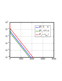
Figure 4: Convergence rate with an I0-error of ±20%plus-or-minuspercent20\pm 20\%. (left) old projection operator (right) new projection operator. (bottom) reconstruction from data with I0-error, and solution (reconstruction using the new projection operator is within the computer numerical precision, i.e. the figure on the right looks identical to the exact solution.
Refer to caption
(a) 8×\times8 frames
Refer to caption
(b) 16×\times16 frames
Refer to caption
(c) 32×\times32 frames
Refer to caption
(d) 64×\times64 frames
Refer to caption
(e) 8×\times8 frames
Refer to caption
(f) 16×\times16 frames
Refer to caption
(g) 32×\times32 frames
Refer to caption
(h) 64×\times64 frames
Figure 5: Convergence rate (εFsubscript𝜀𝐹\varepsilon_{F}, εQsubscript𝜀𝑄\varepsilon_{Q}, ε0subscript𝜀0\varepsilon_{0} vs number of iteration \ell) for (top) regular reconstruction. (bottom) using augmented projection (m=16𝑚16m=16 and step size x1x2=3subscript𝑥1subscript𝑥23x_{1}-x_{2}=3)
Refer to caption
Refer to caption
Refer to caption
Refer to caption
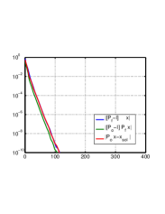
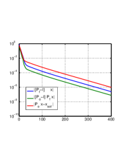
Figure 6: Convergence rate with incoherent illumination of 4 beams, separated by 3×3\times the probe width (FWHM) using standard projection algorithms (top left), with intermediate phase optimization (top-right), phase and amplitude(bottom-left), and phase and amplitude with initial amplitude error of 20% (bottom right), frame width 16×16161616\times 16, 16×16161616\times 16 frames, step size 3.53.53.5 pixels close packing with ±1plus-or-minus1\pm 1 pixel known random perturbations.
Refer to caption
Figure 7: Reconstruction with position errors using the method described in section IV, where εξ0=ξξ0/ξ0subscript𝜀subscript𝜉0norm𝜉subscript𝜉0normsubscript𝜉0\varepsilon_{\xi_{0}}=\|\xi-\xi_{0}\|/\|\xi_{0}\|, and the perturbations in position are randomly distributed with ξ0=1kiξi=2.5delimited-⟨⟩subscript𝜉01𝑘subscript𝑖normsubscript𝜉𝑖2.5\langle\xi_{0}\rangle=\tfrac{1}{k}\sum_{i}\|\xi_{i}\|=2.5 resolution elements. (number of frames: 16×\times16, frame dimensions 32×32323232\times 32, step size: 3.5 pixels, hexagonal packing with known random perturbations of ±1plus-or-minus1\pm 1 pixels and unknown ξ𝜉\xi random perturbations ).
Refer to caption
Refer to caption
Figure 8: Two measured intensities with additive background (SNR=0.5). In a separate test the diffraction data was buried by the background ( (in other figures not included background was 106×10^{6}\times the signal).
Refer to caption
Refer to caption
Refer to caption
Refer to caption
Figure 9: (top) reconstructed image with background optimization (left) and without (right). The figure on the left looks identical to the exact solution. (bottom) reconstructed background (left), convergence behavior(right).
Refer to caption
Figure 10: Fourier transform of the probe w𝑤w used to simulate the experiment

Refer to caption

Figure 11: Map of 11+σ211superscript𝜎2\frac{1}{1+\sigma^{2}}. The σ𝜎\sigma are \infty on dark pixels and 00 on white pixels.
Refer to caption
Figure 12: Convergence behavior with missing data. Frame size: 32×32323232\times 32, number of frames: 16×16161616\times 16, step size: 3.53.53.5 pixels

References

  • [1] W. Hoppe. Beugung im inhomogenen Primärstrahlwellenfeld. I. Prinzip einer Phasenmessung von Elektronenbeungungsinterferenzen. Acta Crystallographica Section A, 25(4):495–501, Jul 1969.
  • [2] R. Hegerl and W. Hoppe. Dynamic theory of crystalline structure analysis by electron diffraction in inhomogeneous primary wave field. Berichte Der Bunsen-Gesellschaft Fur Physikalische Chemie, 74:1148, 1970.
  • [3] J. M. Rodenburg and R. H. T. Bates. The theory of super-resolution electron microscopy via wigner-distribution deconvolution. Phil. Trans. R. Soc. Lond. A, 339:521–553, 1992.
  • [4] John CH Spence. High-resolution electron microscopy, volume 60. Clarendon Press, 2003.
  • [5] Ch. Broennimann, E. F. Eikenberry, B. Henrich, R. Horisberger, G. Huelsen, E. Pohl, B. Schmitt, C. Schulze-Briese, M. Suzuki, T. Tomizaki, H. Toyokawa, and A. Wagner. The pilatus 1m detector. Journal of Synchrotron Radiation, 13(2):120–130, 2006.
  • [6] D. Doering, Y.-D. Chuang, N. Andresen, K. Chow, D. Contarato, C. Cummings, E. Domning, J. Joseph, J. S. Pepper, B. Smith, G. Zizka, C. Ford, W. S. Lee, M. Weaver, L. Patthey, J. Weizeorick, Z. Hussain, and P. Denes. Development of a compact fast ccd camera and resonant soft x-ray scattering endstation for time-resolved pump-probe experiments. Review of Scientific Instruments, 82(7):073303, 2011.
  • [7] H. N. Chapman. Phase-retrieval x-ray microscopy by wigner -distribution deconvolution. Ultramicroscopy, 66:153–172, 1996.
  • [8] P. Thibault, M. Dierolf, A. Menzel, O. Bunk, C. David, and F. Pfeiffer. High-Resolution scanning x-ray diffraction microscopy. Science, 321(5887):379–382, 2008.
  • [9] P. Thibault, M. Dierolf, O. Bunk, A. Menzel, and F. Pfeiffer. Probe retrieval in ptychographic coherent diffractive imaging. Ultramicroscopy, 109:338–343, 2009.
  • [10] J. M. Rodenburg and H. M. L. Faulkner. A phase retrieval algorithm for shifting illumination. Appl. Phy. Lett., 85:4795–4797, 2004.
  • [11] C.M. Kewish, P. Thibault, M. Dierolf, O. Bunk, A. Menzel, J. Vila-Comamala, K. Jefimovs, and F. Pfeiffer. Ptychographic characterization of the wavefield in the focus of reflective hard x-ray optics. Ultramicroscopy, 110:325–9, Mar 2010.
  • [12] Susanne Hönig, Robert Hoppe, Jens Patommel, Andreas Schropp, Sandra Stephan, Sebastian Schöder, Manfred Burghammer, and Christian G. Schroer. Full optical characterization of coherent x-ray nanobeams by ptychographic imaging. Opt. Express, 19(17):16324–16329, Aug 2011.
  • [13] Manuel Guizar-Sicairos, Suresh Narayanan, Aaron Stein, Meredith Metzler, Alec R. Sandy, James R. Fienup, and Kenneth Evans-Lutterodt. Measurement of hard x-ray lens wavefront aberrations using phase retrieval. Applied Physics Letters, 98(11):111108, 2011.
  • [14] M. Guizar-Sicairos and J. R. Fienup. Phase retrieval with transverse translation diversity: a nonlinear optimization approach. Opt. Express, 16:7264–7278, 2008.
  • [15] A.M. Maiden, M.J. Humphry, M.C. Sarahan, B. Kraus, and J.M. Rodenburg. An annealing algorithm to correct positioning errors in ptychography. Ultramicroscopy, 120(0):64 – 72, 2012.
  • [16] Mike Beckers, Tobias Senkbeil, Thomas Gorniak, Klaus Giewekemeyer, Tim Salditt, and Axel Rosenhahn. Drift correction in ptychographic diffractive imaging. Ultramicroscopy, 126(0):44 – 47, 2013.
  • [17] Samuel T Thurman and James R Fienup. Phase retrieval with signal bias. JOSA A, 26(4):1008–1014, 2009.
  • [18] Manuel Guizar-Sicairos and James R. Fienup. Measurement of coherent x-ray focusedbeams by phase retrieval with transversetranslation diversity. Opt. Express, 17(4):2670–2685, Feb 2009.
  • [19] P. Thibault and M. Guizar-Sicairos. Maximum-likelihood refinement for coherent diffractive imaging. New Journal of Physics, 14(6):063004, 2012.
  • [20] Pierre Godard, Marc Allain, Virginie Chamard, and John Rodenburg. Noise models for low counting rate coherent diffraction imaging. Opt. Express, 20(23):25914–25934, Nov 2012.
  • [21] N. C. Jesse and G. P. Andrew. Simultaneous sample and spatial coherence characterisation using diffractive imaging. Applied Physics Letters, 99(15):154103, 2011.
  • [22] J. R. Fienup, J. C. Marron, T. J. Schulz, and J. H. Seldin. Hubble space telescope characterized by using phase-retrieval algorithms. Appl. Opt., 32(10):1747–1767, Apr 1993.
  • [23] Brian Abbey, Keith A. Nugent, Garth J. Williams, Jesse N. Clark, Andrew G. Peele, Mark A. Pfeifer, Martin de Jonge, and Ian McNulty. Keyhole coherent diffractive imaging. Nature Physics, 4:394–398, 03 2008.
  • [24] L. W. Whitehead, G. J. Williams, H. M. Quiney, D. J. Vine, R. A. Dilanian, S. Flewett, K. A. Nugent, A. G. Peele, E. Balaur, and I. McNulty. Diffractive imaging using partially coherent x rays. Phys. Rev. Lett., 103:243902, Dec 2009.
  • [25] Jinsong Wu, Kurt Leinenweber, John CH Spence, and Michael O’Keeffe. Ab initio phasing of x-ray powder diffraction patterns by charge flipping. Nature materials, 5(8):647–652, 2006.
  • [26] J. M. Rodenburg. Ptychography and related diffractive imaging methods. Advances in Imaging and Electron Physics, 150, 2008.
  • [27] H. M. L. Faulkner and J. M. Rodenburg. Movable aperture lensless transmission microscopy: a novel phase retrieval algorithm. Phy. Rev. Lett., 93:023903, 2004.
  • [28] M. Dierolf, A. Menzel, P. Thibault, P. Schneider, C. M. Kewish, R. Wepf, O. Bunk, and F. Pfeiffer. Ptychographic x-ray computed tomography at the nanoscale. Nature, 467:436–439, 2011.
  • [29] Z. Wen, C. Yang, X. Liu, and S. Marchesini. Alternating direction methods for classical and ptychographic phase retrieval. Inverse Problems, 28(11):115010, 2012.
  • [30] C. Yang, J. Qian, A. Schirotzek, F. Maia, and S. Marchesini. Iterative algorithms for ptychographic phase retrieval. Technical Report 4598E, arXiv:1105.5628, Lawrence Berkeley National Laboratory, 2011.
  • [31] J. Qian, C. Yang, A. Schirotzek, F. Maia, and S. Marchesini. Iefficient algorithms for ptychographic phase retrieval. Contemporary Mathematics, to appear, 2013.
  • [32] E. J. Candes, T. Strohmer, and V. Voroninski. Phaselift: Exact and stable signal recovery from magnitude measurements via convex programming. Communications on Pure and Applied Mathematics, 66(8):1241–1274, 2013.
  • [33] H. Ohlsson, A. Y. Yang, R. Dong, and S. Shankar Sastry. Compressive phase retrieval from squared output measurements via semidefinite programming. IEEE Conference on Decision and Control, CDC 2012, November 2011.
  • [34] E. J. Candes, Y. Eldar, T. Strohmer, and V. Voroninski. Phase retrieval via matrix completion. ArXiv e-prints, September 2011.
  • [35] I. Waldspurger, A. d’Aspremont, and S. Mallat. Phase recovery, MaxCut and complex semidefinite programming. ArXiv, June 2012.
  • [36] Zaiwen Wen, Donald Goldfarb, and Katya Scheinberg. Block coordinate descent methods for semidefinite programming. In Miguel F. Anjos and Jean B. Lasserre, editors, Handbook on Semidefinite, Conic and Polynomial Optimization, volume 166 of International Series in Operations Research & Management Science, pages 533–564. Springer US, 2012.
  • [37] J. R. Fienup. Phase retrieval algorithms: a comparison. Appl. Opt., 21:2758–2769, 1982.
  • [38] R. Luke. Relaxed averaged alternating reflections for diffraction imaging. Inverse Problems, 21:37–50, 2005.
  • [39] A. Singer. Angular synchronization by eigenvectors and semidefinite programming. Applied and Computational Harmonic Analysis, 30(1):20 – 36, 2011.
  • [40] Pierre Thibault and Andreas Menzel. Reconstructing state mixtures from diffraction measurements. Nature, 494(7435):68–71, 2013.
  • [41] R. B. Lehoucq, D. C. Sorensen, and C. Yang. Arpack users guide: Solution of large scale eigenvalue problems by implicitly restarted arnoldi methods., 1997.