Cartography of high-dimensional flows: A visual guide to sections and slices

Abstract

Symmetry reduction by the method of slices quotients the continuous symmetries of chaotic flows by replacing the original state space by a set of charts, each covering a neighborhood of a dynamically important class of solutions, qualitatively captured by a ‘template’. Together these charts provide an atlas of the symmetry-reduced ‘slice’ of state space, charting the regions of the manifold explored by the trajectories of interest. Within the slice, relative equilibria reduce to equilibria and relative periodic orbits reduce to periodic orbits. Visualizations of these solutions and their unstable manifolds reveal their interrelations and the role they play in organizing turbulence/chaos.

Today, it is possible to take a stroll through the high-dimensional state space of hydrodynamic turbulence and observe that turbulent trajectories are guided by close passes to invariant solutions of the Navier-Stokes equations. Charting how close these passes are is a geometer’s task, but in order to place them on a map, one first has to deal with families of solutions equivalent under the symmetries of a given flow. Evolution in time decomposes the state space into a ‘spaghetti’ of time trajectories. Continuous spatial symmetries foliate it like the layers of an onion. In this visual tour of dynamics, we use a low-dimensional flow to illustrate how this tangle can be unraveled (symmetry reduction), and how to pick a single representative point for each trajectory (section it) and group orbit (slice it). Once the symmetry induced degeneracies are out of the way, one can identify and describe the prominent turbulent structures by a taxonomy of invariant building blocks (numerically exact solutions of the Navier-Stokes equations, finite sets of relative equilibria and infinite hierarchies of relative periodic orbits) and describe the dynamics in terms of near passes to their heteroclinic connections.

I Introduction

Over the last decade, new insights into the dynamics of moderate Re turbulent flows Faisst and Eckhardt (2003); Wedin and Kerswell (2004); Hof et al. (2004); Kerswell (2005) have been gained through visualizations of their $\infty$-dimensional state spaces by means of dynamically invariant, representation independent coordinate frames constructed from physically prominent unstable coherent structures, Gibson, Halcrow, and Cvitanović (2008) hereafter referred to as templates. Navigating and charting the geometry of these extremely high-dimensional state spaces necessitates a reexamination of two of the basic tools of the theory of dynamical systems: Poincaré sections and symmetry reduction.

In quantum-mechanical calculations, one always starts out by making sure that the Hamiltonian has been brought to its symmetry-reduced block-diagonal, irreducible form; anything else would be sheer masochism. As the dynamical theory of turbulence is still in its infancy, symmetry reduction is not yet a common practice in processing turbulence data collected in experimental measurements and numerical simulations. Symmetry reduction of nonlinear flows is much trickier than the more familiar theory of irreducible representations for linear problems such as quantum mechanics, so most of our sketches illustrate the simplest case, the 1-parameter compact continuous group $\textrm{SO}(2)$ symmetry.

We show here how to bring the numerical or experimental data to a symmetry-reduced format before any further analysis of it takes place. Our tool of choice is the linear implementation of the method of slices. Rowley and Marsden (2000); Beyn and Thümmler (2004); Siminos and Cvitanović (2011); Froehlich and Cvitanović (2011) Here, we extend this local method to a global reduction of a turbulent flow by defining local ‘charts’, their borders, and the ridges that glue these linear tiles into an atlas that spans the ergodic state space region of interest. While ‘charts’ and ‘atlases’ are standard tools in geometry, the prescription for explicit construction of a symmetry-reduced state space presented here is, to our knowledge, new. We explain the key geometrical ideas in simple but illustrative settings, eschewing the fluid dynamical and group theoretical technicalities.

(a)   (b)
(c)   (d)

Figure 1: (a) In the presence of an $N$-continuous parameter symmetry, each state space point $x$ owns $(N\!+\!1)$ tangent vectors: one $v(x)$ along the time flow $x(\tau)$, and the $N$ group tangents $t_{1}(x),\,t_{2}(x),\,\cdots,t_{N}(x)$ along infinitesimal symmetry shifts, tangent to the $N$-dimensional group orbit ${\cal M}_{x}$. (b) Each point has a unique trajectory (blue) under time evolution. (c) Each point also belongs to a group orbit (green) of symmetry-related points. For $\textrm{SO}(2)$, this is topologically a circle. Any two points on a group orbit are physically equivalent, but may lie far from each other in state space. (d) Together, time-evolution and group actions trace out a wurst of physically equivalent solutions.

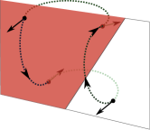
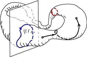
Let us begin by defining a dynamical system comprised of a flow $f^{t}$ and the state space ${\cal M}$ on which it acts. If a group $G$ of continuous transformations acts on a continuous time flow, each state space point owns a set of tangent vectors (Fig. 1 (a)). Integrated in time, the velocity vector $v(x)$ traces out a trajectory ${f^{\tau}(x)}$ (Fig. 1 (b)). Applying the continuous transformations traces out a group orbit ${\cal M}_{x}=\{g\,x\mid g\in{G}\}\,$ (Fig. 1 (c)). Together, time evolution and group actions trace out a complicated smooth manifold, hereafter affectionately referred to as a wurst (see Figs. 1 (d), 4 (b) and 8), which we shall here teach you how to slice.

A flow is said to have symmetry $G$ if the form of evolution equations $\dot{x}=v(x)$ is left invariant, $v(x)=g^{-1}\,v(g\,x)\,,$ by the set of transformations $g\in{G}$. If a flow has symmetry, the simplest solutions are highly symmetric invariant equilibria and relative equilibria studied in bifurcation-theory approaches to the onset of turbulence. Physicists love symmetries, Kerswell (2012) but nature often prefers solutions of no symmetry: while the flow equations may be invariant under $G$, turbulent solutions are not. The highly symmetric solutions often lie far from the regions of state space explored by turbulence Willis, Cvitanović, and Avila (2012) and thus are of limited usefulness in understanding its dynamics. In contrast, the relative periodic orbits studied here are embedded in the turbulence, and capture its geometry and statistics.

We can make headway in unraveling the tangle of 1-dimensional time trajectories with the notion of recurrence. To quantify how close the state of the system at a given time is to a previously visited state, we need the notion of distance between two points in state space. The simplest (but far from the only, or the most natural) is the Euclidean norm

$$\|{x-x^{\prime}}\|^{2}=\langle{x-x^{\prime}}\vphantom{x-x^{\prime}}|\vphantom{x-x^{\prime}}{x-x^{\prime}}\rangle=\sum_{i=1}^{d}(x-x^{\prime})_{i}^{2}\,.$$ (1)

For experimental data, a better norm, for example, might be a distance between digitized images. While in this paper we simply assume that a norm is given, its importance cannot be overstated: the construction of invariant, PDE discretization independent state space coordinates, Gibson, Halcrow, and Cvitanović (2008) the symmetry reduction by minimization of the distance between group orbits undertaken in what follows, and the utility of the charts so constructed all depend on a well-chosen notion of distance in the high-dimensional state spaces we are charting here.

Given a notion of distance, we can talk about a ‘neighborhood’, an open set of nearby states with qualitatively similar dynamics. Our main task in what follows will be to make this precise by defining a chart over a neighborhood and its borders. Given distances and neighborhoods, the next key notion is measure, or how likely a typical trajectory is to visit a given neighborhood. After some observations of a given turbulent flow, one can identify a set of templates, Rowley and Marsden (2000) points ${\hat{x}^{\prime}}{}^{(j)}$, $j=1,2,\cdots$ in the state space representative of the most frequently revisited features of the flow.

Our goals here are two-fold: (i) In sect. II, we review the method of Poincaré sections, with emphasis on two particular aspects that are applicable to high-dimensional flows: the construction of multiple local linear charts and the determination of their borders. (ii) In sect. III, we discuss the effect of continuous symmetries on nonlinear flows, and in sect. IV we use the lessons learned from our discussion of Poincaré sections to aid us in the reduction of continuous symmetries, and, thus, enable us to commence a systematic charting of the long-time dynamics of high-dimensional flows (sect. V).

II Section

In the Poincaré section method, one records the coordinates $\hat{x}_{n}$ of the trajectory $x(\tau)$ at the instants $\tau_{n}$ when it traverses a fixed oriented hypersurface ${\cal P}$ of codimension 1. For the high-dimensional flows that we have in mind, the practical choice is a hyperplane, the only type of Poincaré section (from now on, just a section) that we shall consider here. One can choose a section such that it contains a template of interest. Properly oriented, such a section can capture important features of the flow in the neighborhood of the section-fixing template.

But how far does this neighborhood extend? The answer is that the section captures neighboring trajectories as long as it cuts them transversally; it fails the moment the velocity field at a point $\hat{x}^{\ast}$ fails to pierce the section. At these locations, the velocity either vanishes (equilibrium) or is orthogonal to the section normal $\hat{n}$,

$$\hat{n}\cdot v(\hat{x}^{\ast})=0\,,\qquad\hat{x}^{\ast}\in\cal{S}\,.$$ (2)

For a smooth flow in $d$ dimensions such points form a smooth $(d\!-\!2)$-dimensional section border ${\cal S}\subset{\cal P}$, which encloses the open neighborhood of the template characterized by qualitatively similar flow. We shall refer to this region of the section as a chart of the template neighborhood (see Fig. 2). Beyond the border, the flow pierces the section in the ‘wrong’ direction and the dynamics are qualitatively different.

As an example consider the Rössler system Rössler (1976),

$$\begin{split}\dot{x}&=-y\,-\,z\\ \dot{y}&=x+ay\\ \dot{z}&=b+z(x-c)\,,\end{split}$$ (3)

where $a=b=0.2$ and $c=5.7$. This flow has two prominent invariant states, the ‘inner’ and the ‘outer’ unstable equilibria ${\hat{x}^{\prime}}{}^{(-)}$ and ${\hat{x}^{\prime}}{}^{(+)}$ (see Fig. 2 (a)) , which we choose as templates for our sections.

We orient the sections so the plane ${\cal P}_{-}$ contains ${\hat{x}^{\prime}}{}^{(-)}$ and its 1-dimensional stable eigenvector (Fig. 2 (b)), and the other section ${\cal P}_{+}$ contains ${\hat{x}^{\prime}}{}^{(+)}$ and its 1-dimensional unstable eigenvector (Fig. 2 (c)), thus capturing the local spiral-in, spiral-out dynamics. The remaining freedom to rotate each section can be used to orient them in such a way that the ridge (the intersection of the two sections) lies approximately between the two templates (Fig. 2 (d)). Choosing sections is a dark art: in the example at hand the dynamics of interest is captured by the two charts - if that were not the case, one would have had to interpolate, by inserting a third chart between them.

(a) (b)

(c) (d)

Figure 2: 2-chart atlas for Rössler flow. (a) The inner equilibrium ${\hat{x}^{\prime}}{}^{(-)}$ is a (spiral-out) saddle-focus with a 2-dimensional unstable manifold and a 1-dimensional stable manifold. The outer equilibrium ${\hat{x}^{\prime}}{}^{(+)}$ is a (spiral-in) saddle-focus, with a 2-dimensional stable manifold (basin boundary for initial conditions that either fall into the chaotic attractor, or escape to infinity) and a 1-dimensional unstable manifold. (b) Chart ${\cal P}_{-}$ of the ${\hat{x}^{\prime}}{}^{(-)}$ neighborhood carved out of a Poincaré section plane through the inner equilibrium ${\hat{x}^{\prime}}{}^{(-)}$ and its stable eigenvector, with section border drawn as the solid red line. Note the ridge (dashed blue line): the chart stops at the ridge. (c) Chart ${\cal P}_{+}$ (here viewed from below) is bounded by section border (solid red line) of a section through the outer equilibrium ${\hat{x}^{\prime}}{}^{(+)}$ and its unstable eigenvector. The chart stops at the ridge (dashed blue line), and it does not intersect the strange attractor. (d) A two-chart atlas of Rössler flow, with charts ${\cal P}_{-}$ and ${\cal P}_{+}$ oriented and combined so that the ridge (intersection of the two sections, indicated by the dashed blue line in the three figures) lies approximately between the templates. Section hyperplanes beyond this ridge do not belong to the atlas.

For Rössler flow, the border condition (2) yields a quadratic condition in 3 dimensions, so the section borders drawn in Fig. 2 (b) and Fig. 2 (c) are conic sections. The two charts meet at a ridge, and together do a pretty good job as the 2-chart atlas of the interesting Rössler dynamics. Due to the extreme contraction rate of the attractor, its intersection with the section in Fig. 2 (b) is for all practical purposes 1-dimensional, and the associated return map yields all periodic orbits of the 3-dimensional flow. Cvitanović et al. (2012)

In 3 dimensions everything —sections, ridges, section borders— can be drawn and the chart fits on a 2-dimensional sheet of papyrus. But what about for hydrodynamic flows where the dimensionality $d$ of the state space is very large? The point of the cartographical enterprize undertaken here is that while it is impossible to visualize the $(d\!-\!2)$-dimensional section border of the $(d\!-\!1)$-dimensional slab that is now our chart, Gibson and Cvitanović (2012) a point is a point and a line is a line in a projection from any number of dimensions, so a trajectory crossing of either a section or a section border can be easily determined and visualized in any dimension.

To summarize: Evolution in time decomposes the state space into a spaghetti of 1-dimensional trajectories $x(\tau)$, each fixed by picking a single point $x(0)$ on it. A well chosen set of section charts of codimension 1 allows us to ‘quotient’ the continuous time parameter $\tau$, and reveal the dynamically important transverse structure of the flow’s stable/unstable manifolds. For unstable trajectories one needs, in addition, a notion of recurrence to the section. The set of points $\{\hat{x}_{n}\}=\{x(\tau_{n})\}$, separated by short time flights in between sections, captures the transverse dynamics without losing any information about the chaotic flow. We can thus chart interesting regions of state space by picking a sufficient number of templates and using them to construct charts of their neighborhoods, each bounded by section borders and ridges.

We close this section with a remark on what sections are not: A Poincaré section is not a projection onto a lower-dimensional space (in sense that a photograph is a 2-dimensional projection of a 3-dimensional space). Rather, it is a local change of coordinates to a direction along the flow $v(\hat{x})$, and the remaining coordinates transverse to it. No information about the flow is lost; the full space trajectory $x(\tau)$ can always be reconstructed by integration from its point $\hat{x}$ in the section.

III Dancers and drifters

(a) (b)

(c) (d)

Figure 3: A symmetry relates physically equivalent states; a pipe flow solution translated or rotated is also a solution. (a) An instantaneous state of the fluid is indicated by a ‘swirl’ - here the reader has to imagine a particular instantaneous velocity field across the entire pipe. The same state may be rigidly (b) translated by downstream shift $\ell$ (fluid states are $\textrm{SO}(2)_{z}$ equivariant in a stream-wise periodic pipe), (c) translated by $\ell$ and rotated azimuthally by ${\bf\phi}$ (the two states are $\textrm{SO}(2)_{\theta}\times\textrm{SO}(2)_{z}$ equivariant), and (d) reflected and rotated azimuthally by ${\bf\phi}$ (the two states are $\textrm{O}(2)_{\theta}$ equivariant). Some symmetry-related states may also be connected by time evolution. A relative equilibrium is a solution of the equations of motion that retains its shape while rotating and traveling downstream with constant phase velocity $c$. A relative periodic orbit ${\cal M}_{p}$ is a time dependent, shape-changing state of the fluid that after a period ${T_{p}}$ reemerges as (b), (c), or (d), the initial state translated by $\ell_{p}$, rotated by ${\bf\phi}_{p}$ and possibly also azimuthally reflected.

What is a symmetry? A visualization of the fluid dynamics of a pipe flow, Fig. 3, affords an intuitive illustration. Solutions of pipe flow remain physically the same under azimuthal rotations and stream-wise translations (which become $\textrm{SO}(2)$ rotations in numerical stream-wise periodic pipes), but rotated and shifted solutions may correspond to distant points in state space.

Each $\textrm{SO}(2)$ group orbit is topologically a circle, but it traces out a complicated state space curve composed of many Fourier modes that are nonlinearly coupled and thus of comparable magnitude. Together, the two $\textrm{SO}(2)$ symmetries of numerical pipe flow sweep out contorted and hard to visualize $T^{2}$ tori (see ref. Willis, Cvitanović, and Avila (2012)), so we shall illustrate the key ideas by a much simpler example, the $\textrm{SO}(2)$-equivariant Gibbon and McGuinness Gibbon and McGuinness (1982); Fowler, Gibbon, and McGuinness (1982) complex Lorenz equations of geophysics and laser physics,

$$\dot{x}_{1} = -\sigma x_{1}+\sigma y_{1}\,,\qquad\dot{x}_{2}\,=\,-\sigma x_{2}+\sigma y_{2}$$

$$\dot{y}_{1} = (\rho_{1}-z)x_{1}-\rho_{2}x_{2}-y_{1}-ey_{2}$$

$$\dot{y}_{2} = \rho_{2}x_{1}+(\rho_{1}-z)x_{2}+ey_{1}-y_{2}$$

$$\dot{z}\; = -bz+x_{1}y_{1}+x_{2}y_{2}\,.$$ (4)

Here all coordinates and parameters are real. In our calculations the parameters are set to those used by Siminos’ Siminos (2009) $\rho_{1}=28,\,\rho_{2}=0,\,b=8/3,\,\sigma=10,\,e=1/10$. The complex Lorenz equations are an example of a simple dynamical system with a continuous (but no discrete) symmetry, equivariant under $\textrm{SO}(2)$ rotations by

$$g({\bf\phi}) = \exp{({{\bf\phi}}\mathbf{T})}\,=\,\left(\begin{array}[]{ccccc}\cos{\bf\phi}&\sin{\bf\phi}&0&0&0\\ -\sin{\bf\phi}&\cos{\bf\phi}&0&0&0\\ 0&0&\cos{\bf\phi}&\sin{\bf\phi}&0\\ 0&0&-\sin{\bf\phi}&\cos{\bf\phi}&0\\ 0&0&0&0&1\end{array}\right)$$ (10)

The group is 1-dimensional and compact, its elements parameterized by ${\bf\phi}\mbox{ mod }2\pi$. For historical background, Poincaré return maps, symbolic dynamics and in-depth investigation of the model, see refs. Siminos (2009); Siminos and Cvitanović (2011).

(a) (b)

(c) (d)

Figure 4: Complex Lorenz flow, $d=5\to 3$ dimensional $\{x_{1},x_{2},z\}$ projections: (a) The strange attractor. (b) The initial relative equilibrium $TW_{1}$ point is shown by the red dot, and its group orbit / trajectory by the dashed red line. One period of the $\overline{01}$ relative periodic orbit is shown by the solid blue line. The group orbit of its (arbitrary) starting point is shown by the dashed blue line: after one period the trajectory has returned to the group orbit but with a different phase. The wurst, i.e., the group orbit of the $\overline{01}$ trajectory (dark blue) is shown by the cyan surface. Following $\overline{01}$ for 15 more periods (faint dotted lines) starts filling out this torus; in that time, the slowly drifting relative equilibrium $TW_{1}$ has advanced to the next red dot (red line). Symmetry-reduced complex Lorenz flow, $d=4\to 3$ dimensional $\{x_{2},y_{2},z\}$ projections: (c) Strange attractor from frame (a) reduced to a single slice hyperplane, using $TW_{1}$ as the template. $\overline{01}$ is now a periodic orbit, shown by the solid black line. The dynamics exhibits singular jumps (shown in red) due to forbidden crossings of the chart border. In contrast to the 1-dimensional section borders of Fig. 2, here the chart borders are 3-dimensional and hard to visualize. (d) The 2-chart atlas (see the sketch of Fig. 11) of the same strange attractor encounters no chart borders and exhibits no singularities. The trajectory changes colors from red to blue as it crosses between the slice hyperplanes of ${\hat{x}^{\prime}}{}^{(1)}$ and ${\hat{x}^{\prime}}{}^{(2)}$. The ridge (shown in brown) acts as a Poincaré section ${\cal P}$ with red or blue ridge points $\hat{x}^{*}$ marking the direction of the crossing. The charts are 4-dimensional, the ridge 3-dimensional, so the colored blocks and planes are only cartoon drawings of their projections onto the 2-dimensional figure.

The strange attractor of the complex Lorenz flow , in its present state, is a complete mess (Fig. 4 (a)). Solutions tend to drift along continuous symmetry directions, with the physically important shape-changing dynamics hidden from view.

The ultimate drifter, the signature invariant solution that signals the presence of a continuous symmetry is a relative equilibrium (traveling wave, rotational wave, etc.), a trajectory whose velocity field lies within the group tangent space, $v(x)=c\cdot t(x)\,,$ and whose time evolution is thus confined to the group orbit (see Fig. 4 (b)); think of an unchanging body carried by a stream.

A relative periodic orbit behaves more like a dancer. ${\cal M}_{p}$ is a trajectory that recurs exactly

$$x(\tau)=g_{p}\,x(\tau+{T_{p}})\,,\qquad x(\tau)\in{\cal M}_{p}\,,$$ (11)

after a fixed relative period ${T_{p}}$, but shifted by a fixed group action ${g_{p}}$ that maps the endpoint $x({T_{p}})$ back into the initial point cycle point $x(0)$; think of a dancer moving across the stage through a set of motions and then striking her initial pose, Shapere and Wilczek (2006) or study the pipe flow sketches in Fig. 3.

Because the $\textrm{SO}(2)$ transformations act on the complex Lorenz flow only through the simplest $m=1$ Fourier mode, here all group orbits are circles and appear elliptical in $d=5\to 3$ dimensions projections. Nevertheless, even the wurst traced out by one of the simplest relative periodic orbits $\overline{01}$ Siminos and Cvitanović (2011) (shown in Fig. 4 (b)) is not so easy to get one’s head around: you are looking at a 3-dimensional projection of a torus embedded in 5 dimensions.

(a)     (b)

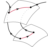
(c) (d)    

Figure 5: (a) The $N$-dimensional group orbit ${\cal M}_{x(0)}$ of state space point $x(0)$ and the group orbit ${\cal M}_{x(\tau)}$ reached by the trajectory $x(\tau)$ a time $\tau$ later. (b) Two physically equivalent trajectories $x(\tau)$ and $\hat{x}(\tau)$ are related, in general, by an arbitrary, time dependent moving frame transformation $g(\tau)$, such that $x(\tau)=g(\tau)\,\hat{x}(\tau)$. (c) A symmetry reduction scheme ${\cal M}\to\hat{\cal M}$ is a rule that prescribes $g(\tau)$ and thus replaces a group orbit ${\cal M}_{x}\subset{\cal M}$ through $x$ by a single point $\hat{x}\in\hat{\cal M}$. (d) In this paper, $g(\tau)$ is fixed variationally by the extremal condition (13) for the point $\hat{x}$ on the group orbit ${\cal M}_{x}$ that is nearest to the template ${\hat{x}^{\prime}}$.

To summarize: continuous symmetries in the dynamics foliate the state space into an onion, where each layer is a group orbit (Fig. 5 (a)). How are we to sort out this mess? All the points on a group orbit are physically equivalent, so we are free to replace a given flow $x(\tau)$ by any other $\hat{x}$($\tau$), such that $x(\tau)=g(\tau)\,\hat{x}(\tau)$ by a moving frame Fels and Olver (1998, 1999); Olver (1999) transformation $g(\tau)$. As long as no symmetry reduction procedure is prescribed, $g(\tau)$ is free: it can be any, in general time dependent, group transformation. For example, to film our dancer, we can mount the camera on a cart moving alongside her. So, in the presence of continuous symmetries, there are two kinds of motion: those of a dancer, continuously changing shapes, and those of a drifter, merely shuffling along the shape invariant directions. We will presently banish the drifters and just enjoy the dance.

IV Chart

Suppose you are computing a set of numerically exact invariant solutions of the Navier-Stokes equations. Do you want to compute the same solution over and over again, once for every point on the group orbit? No, you would like to compute it only once. The strategy for picking out that one representative solution is called symmetry reduction. Its goal is to replace each group orbit by a unique point in a lower-dimensional symmetry-reduced state space $\hat{\cal M}\subset{\cal M}/G$, as sketched in Fig. 5 (c).

What is a smart way to go about it? Intuition gained from pipe flow (see Fig. 3) will again prove helpful. A turbulent flow exhibits a myriad of unstable structures, each traveling down the pipe with its own phase velocity. The method of slices Rowley and Marsden (2000); Beyn and Thümmler (2004); Siminos and Cvitanović (2011); Froehlich and Cvitanović (2011) that we now describe tells you how to pull each solution back into a fixed frame called a slice and compare it to your repertoire of precomputed solutions, or the templates $\{{\hat{x}^{\prime}}{}^{(j)}\}$, using the poor geometer’s version of a geodesic, the principle of the closest distance to each. What follows is similar to the construction of sections of sect. II; due to the linear action of the symmetry group, slicing is easier than sectioning, but wholly unfamiliar. This is why we reviewed the Poincaré sections first. We now offer a pictorial tour of this (save for one bold incursion Willis, Cvitanović, and Avila (2012)) hitherto uncharted territory.

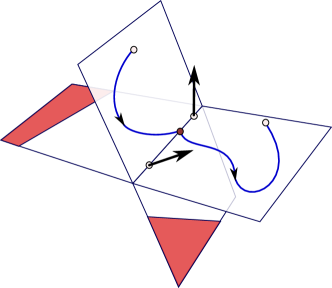
First, pick a template ${\hat{x}^{\prime}}$ and use the freedom to shift and rotate it (Fig. 5 (b)) until it overlies, as well as possible, the state $x$, by minimizing the distance

$$\|{x-g({\bf\phi})\,{\hat{x}^{\prime}}}\|\,.$$ (12)

Now, replace the entire group orbit of $x$ by the closest match to the template pattern, given by $\hat{x}=g^{-1}x$. From here on, we will use the hat on $\hat{x}$ to indicate the unique point on the group orbit of $x$ that is closest to the template $\hat{x}^{\prime}$. The symmetry-reduced state space $\hat{\cal M}$ is comprised of such closest matches, a point for each full state space group orbit.

The minimal distance satisfies the extremum condition (Fig. 5 (d))

$$\frac{\partial}{\partial{\bf\phi}}\|{x-g({\bf\phi})\,{\hat{x}^{\prime}}}\|^{2}=2\,\langle{\hat{x}-{\hat{x}^{\prime}}}\vphantom{t^{\prime}}|\vphantom{\hat{x}-{\hat{x}^{\prime}}}{t^{\prime}}\rangle=0\,,\quad t^{\prime}=\mathbf{T}{\hat{x}^{\prime}}\,,$$

where the $[d\!\times\!d]$ matrix $\mathbf{T}$ is the generator of infinitesimal symmetry transformations. $\|{g({\bf\phi}){\hat{x}^{\prime}}}\|=\|{{\hat{x}^{\prime}}}\|$ is a constant. To streamline the exposition, we shall assume here that the symmetry group is $\textrm{SO}(n)$. In that case $\mathbf{T}$ is antisymmetric, so the group tangent vector $t^{\prime}$ evaluated at ${\hat{x}^{\prime}}$ is normal to ${\hat{x}^{\prime}}$ and the term $\langle{{\hat{x}^{\prime}}}\vphantom{\mathbf{T}\,{\hat{x}^{\prime}}}|\vphantom{{\hat{x}^{\prime}}}{\mathbf{T}\,{\hat{x}^{\prime}}}\rangle$ vanishes. Therefore $\hat{x}$, the point on the group orbit of $x$ that lands in the slice satisfies the slice condition

$$\langle{\hat{x}}\vphantom{t^{\prime}}|\vphantom{\hat{x}}{t^{\prime}}\rangle=0\,.$$ (13)

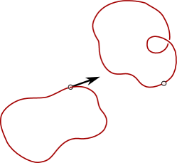
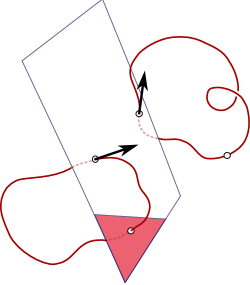
As $x(\tau)$ varies in time, the template ${\hat{x}^{\prime}}$ tracks the motion using the slice condition (13) to minimize $\|{x(\tau)-g(\phi(\tau)){\hat{x}^{\prime}}}\|$, and the full-space trajectory $x(\tau)$ is rotated into the reduced state space trajectory $\hat{x}(\tau)$ by appropriate time varying moving frame angles $\{{\bf\phi}(\tau)\}$, as depicted in Fig. 6 (a). $\hat{\cal M}$ is thus a $(d\!-\!N)$-dimensional hyperplane normal to the $N$ group tangents evaluated at the $\hat{x}^{\prime}$ as sketched in Fig. 6 in a highly idealized manner: A group orbit is an $N$-dimensional manifold and, even for $\textrm{SO}(2)$, is usually only topologically a circle and can intersect a hyperplane any number of times (see Figs. 7 and 8).

(a)

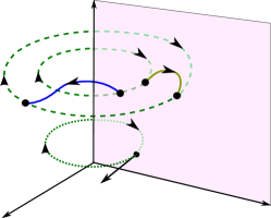
(b)

Figure 6: The method of slices, a state space visualization: (a) A chart $\hat{\cal M}\subset{\cal M}/G$ lies in the $(d\!-\!N)$-dimensional slice hyperplane (13) normal to $t^{\prime}_{1}...t^{\prime}_{N}$, which span the $N$-dimensional space tangent to the group orbit $g\,{\hat{x}^{\prime}}$ (dotted line) evaluated at the template point ${\hat{x}^{\prime}}$. The hyperplane intersects all full state space group orbits (green dashes). The full state space trajectory $x(\tau)$ (blue) and the reduced state space trajectory $\hat{x}(\tau)$ (green) are equivalent up to a ‘moving frame’ rotation $x(\tau)=g(\tau)\,\hat{x}(\tau)$, where $g(\tau)$ is a shorthand for $g({\bf\phi}(\tau))$. (b) In the full state space, a relative periodic orbit $x(0)\to x(\tau)\to x({T_{p}})$ returns to the group orbit of $x(0)$ after a time ${T_{p}}$, such that $x(0)=g_{p}x({T_{p}})$. A generic relative periodic orbit quasi-periodically fills out what is topologically a torus (Fig. 4 (b)). In the slice, the symmetry-reduced trajectory is periodic, $\hat{x}(0)=\hat{x}({T_{p}})$.

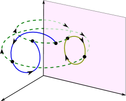
One can write the equations for the flow in the reduced state space $\dot{\hat{x}}=\hat{v}(\hat{x})$ (for details see, for example, ref. Cvitanović et al. (2012)) as

$$\hat{v}(\hat{x}) = v(\hat{x})\,-\,\dot{{\bf\phi}}(\hat{x})\,t(\hat{x})$$ (14)

$$\dot{{\bf\phi}}(\hat{x}) = \langle{v(\hat{x})}\vphantom{t^{\prime}}|\vphantom{v(\hat{x})}{t^{\prime}}\rangle/\langle{t(\hat{x})}\vphantom{t^{\prime}}|\vphantom{t(\hat{x})}{t^{\prime}}\rangle\,,$$ (15)

which confines the motion to the slice hyperplane. Thus, the dynamical system $\{{\cal M},f^{t}\}$ with continuous symmetry $G$ is replaced by the reduced state space dynamics $\{\hat{\cal M},\hat{f}^{t}\}$: The velocity in the full state space $v$ is the sum of $\hat{v}$, the velocity component in the slice hyperplane, and $\dot{{\bf\phi}}\,t$, the velocity component along the group tangent space. The integral of the reconstruction equation for $\dot{{\bf\phi}}$ keeps track of the group shift in the full state space.

(a)   (b)​​

Figure 7: The chart border  is the $(d\!-\!N\!-1)$-dimensional  hyperplane that contains all the points $\hat{x}^{\ast}$ whose group tangents $t(\hat{x}^{\ast})$ lie in the slice hyperplane or vanish and are thus normal to $t^{\prime}$. Beyond this boundary, the group orbits pierce the slice hyperplane in the wrong direction, so only the half-hyperplane that contains the template belongs to the slice. The chart border is not easy to visualize; For the lack of dimensions, here it is drawn as a ‘line’, the $z$ axis in this 3-dimensional sketch. (a) If the equivariant coordinates transform only under the $m=1$ representation of $\textrm{SO}(2)$, every group orbit is a circle, and crosses any slice hyperplane exactly twice. However, if there are coordinates that transform as higher $m$, the group orbit can pierce the hyperplane up to $2m$ times, and the chart border lies closer to the template: For example, (b) a group orbit for a combination of $m=1$ and $m=2$ equivariant coordinates resembles the seam of a baseball, and can cross the slice hyperplane 4 times, out of which only the point closest to the template is in the slice.

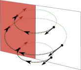
The template ${\hat{x}^{\prime}}$ should be a generic state space point in the sense that its group orbit has the full $N$ dimensions of the group $G$. The set of the group orbit points closest to the template $\hat{x}^{\prime}$ forms a neighborhood of $\hat{x}^{\prime}$ in which each group orbit intersects the hyperplane only once. A slice hyperplane qualitatively captures neighboring group orbits until, for a point $\hat{x}^{\ast}$ not so close to the template, the group tangent vector $t(\hat{x}^{\ast})$ lies in the slice hyperplane. The group orbits for such points are grazed tangentially rather than sliced transversally, much like what happens at the section border (2) for evolution in time. This is also a linear condition and defines the chart border ${\cal S}$, Siminos and Cvitanović (2011); Froehlich and Cvitanović (2011) a $(d\!-\!N\!-1)$-dimensional manifold, which contains all the points $\hat{x}^{\ast}$ whose group tangents lie in the slice hyperplane, i.e.,

$$\langle{\hat{x}^{\ast}}\vphantom{t^{\prime}}|\vphantom{\hat{x}^{\ast}}{t^{\prime}}\rangle\,=\,0\mbox{ and }\langle{t(\hat{x}^{\ast})}\vphantom{t^{\prime}}|\vphantom{t(\hat{x}^{\ast})}{t^{\prime}}\rangle\,=\,0\,.$$ (16)

${\cal S}$ also contains all points for which $t(\hat{x}^{\ast})=0$. While for the Poincaré sections (2) the analogous points were equilibria (captured only if the section cut through them), for slice hyperplanes points with vanishing group actions belong to invariant subspaces, and, by its definition, every chart border automatically includes all invariant subspaces.

Figure 8: Wurst, sliced. Every slice hyperplane cuts every group orbit at least twice (see Fig. 6), once at the orbit’s closest passage to the template, and another time at the most distant passage, also satisfying the slice condition (13). An $\textrm{SO}(2)$ relative periodic orbit ${\cal M}_{p}$ is topologically a torus, so the two cuts are the two periodic orbit images of the same relative periodic orbit, the good close one $\hat{x}_{p}$ (blue), and the bad distant one (red), on the other side of chart border, and thus not in the slice.

For the complex Lorenz equations (4), the invariant subspace is the 1-dimensional $z$-axis, with trivial dynamics, $z=-bz$, but in general invariant subspaces are high-dimensional and have their own dynamics. Physicists, for example general relativists, often work in invariant subspaces, as this is easier than solving the full problem. Cvitanović, Davidchack, and Siminos (2010) Such approaches yield highly symmetric solutions, Stephani et al. (2009); Gibson, Halcrow, and Cvitanović (2009) whose dynamics may be quite different from those that guide turbulence in the full state space (for a striking example, see ref. Willis, Cvitanović, and Avila (2012)).

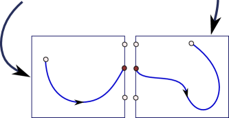
There is yet another, much kinder type of a border: a ridge. Our initial chart $\hat{\cal M}{}^{(1)}$ is a ($d\!-\!N$)-dimensional  hyperplane. If we pick another template point ${\hat{x}^{\prime}}{}^{(2)}$, it comes along with its own slice hyperplane $\hat{\cal M}{}^{(2)}$. Any pair of $(d\!-\!N)$-dimensional  local slice hyperplanes intersects in a ridge, a $(d\!-\!N-\!1)$-dimensional  hyperplane ${\cal P}$ of points $\hat{x}^{*}$ shared by a pair of charts and thus satisfying the slice condition (13) for both,

$$\langle{\hat{x}^{*}}\vphantom{t^{\prime}{}^{(1)}}|\vphantom{\hat{x}^{*}}{t^{\prime}{}^{(1)}}\rangle=0\mbox{ and }\langle{\hat{x}^{*}}\vphantom{t^{\prime}{}^{(2)}}|\vphantom{\hat{x}^{*}}{t^{\prime}{}^{(2)}}\rangle=0\,.$$ (17)

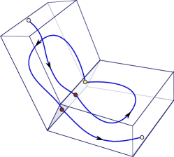
The ridge forms a Poincaré section ${\cal P}{}^{(ij)}$ that serves as a toll bridge, crossed by any direct transit from a chart $\hat{\cal M}{}^{(j)}$ to the adjacent chart $\hat{\cal M}{}^{(i)}$. In Fig. 10 (a) a ridge is visualized as a ‘line’, and in Fig. 11 as a ‘plane’ of intersection of two volumes. We shall refer to the neighborhood of a template ${\hat{x}^{\prime}}{}^{(j)}$ bounded by its chart border and the ridges to other such linear neighborhoods as a chart $\hat{\cal M}{}^{(j)}\subset{\cal M}/G$, and to (16) and (17) as the border conditions.

V Charting the slice

Let us summarize the voyage so far: we are charting a curved manifold, and it would be nice to use tools of differential geometry, but this seems not possible in the high-dimensional state space of hydrodynamics turbulence. The only feasible way to chart this space is to (1) quotient all continuous symmetries, and (2) tile the reduced state space with flat $(d\!-\!N)$-dimensional  tiles, or charts. We do this step by step, starting with a set of templates and using them to construct charts of each neighborhood, and then building up an atlas of the slice, chart by chart, which captures all of the reduced dynamics of interest (but not all possible dynamics). Here are the steps along the way:

Template

Pick a template ${\hat{x}^{\prime}}$ such that $G$ acts on it regularly with a group orbit of dimension $N$.

Slice hyperplane

The $(d\!-\!N)$-dimensional hyperplane satisfying $\langle{\hat{x}}\vphantom{t^{\prime}_{a}}|\vphantom{\hat{x}}{t^{\prime}_{a}}\rangle=0\,,$ normal to group transformation directions at the template ${\hat{x}^{\prime}}$.

Moving frame

For any $x$, the slice condition $\langle{\hat{x}}\vphantom{t^{\prime}}|\vphantom{\hat{x}}{t^{\prime}}\rangle=0$ on $x=g({\bf\phi})\hat{x}$ determines the moving frame, i.e., the group action $g({\bf\phi})$ that brings $x$ into the slice hyperplane.

Chart border

The set of points $\hat{x}^{\ast}$ on a slice hyperplane whose group orbits graze the hyperplane tangentially, such that $\langle{\hat{x}^{\ast}}\vphantom{t^{\prime}}|\vphantom{\hat{x}^{\ast}}{t^{\prime}}\rangle\,=\,\langle{t(\hat{x}^{\ast})}\vphantom{t^{\prime}}|\vphantom{t(\hat{x}^{\ast})}{t^{\prime}}\rangle\,=\,0\,.$

Flow invariant subspace

If a subset or all of the group tangents of a chart border point $\hat{x}^{\ast}$ vanish, $t_{a}(\hat{x}^{\ast})=0$, its time trajectory remains within a flow-invariant subspace for all times.

Ridge

A hyperplane of points $\hat{x}^{*}\in{\cal P}{}^{(21)}$ formed by the intersection of a pair of slice hyperplanes $\hat{\cal M}{}^{(1)}$ and $\hat{\cal M}{}^{(2)}$.

Chart

The neighborhood of a template ${\hat{x}^{\prime}}{}^{(j)}$, bounded by the chart border and the ridges to other linear neighborhoods, comprises a chart $\hat{\cal M}{}^{(j)}\subset{\cal M}/G$. The borders ensure that there is no more than one oriented group orbit traversal per chart; a group orbit either pierces one chart, or no charts at all.

Atlas

A set of $(d\!-\!N)$-dimensional contiguous charts $\hat{\cal M}{}^{(1)},\hat{\cal M}{}^{(2)},\cdots$

Slice

Let $G$ act on a $d$-dimensional manifold ${\cal M}$, with group orbits of dimension $N$ or less. A slice is a $(d\!-\!N)$-dimensional submanifold $\hat{\cal M}$ such that all group orbits that intersect $\hat{\cal M}$ do so transversally and only once.

(a)  

(b)  

Figure 9: A 2-chart atlas. Sketch (a) depicts two templates ${\hat{x}^{\prime}}{}^{(1)}$, $x^{\prime}{}^{(2)}$, each with its group orbit. Start with the template ${\hat{x}^{\prime}}{}^{(1)}$. All group orbits traverse its $(d\!-\!1)$-dimensional slice hyperplane, including the group orbit of the second template $x^{\prime}{}^{(2)}$. (b) Replace the second template by its closest group orbit point ${\hat{x}^{\prime}}{}^{(2)}$, i.e., the point in chart $\hat{\cal M}{}^{(1)}$. This is allowed as long as ${\hat{x}^{\prime}}{}^{(2)}$ is closer than the $\hat{\cal M}{}^{(1)}$ chart border (red region), otherwise an interpolating, closer template needs to be introduced.

(a)  

(b)  

Figure 10: A 2-chart atlas. (a) Now that the group orbits have been reduced to points, erase them and consider the two slice hyperplanes through the two templates. As these two templates are the closest points viewed from either group orbit, they lie in both slice hyperplanes. However, the two tangent vectors $t^{\prime}{}^{(1)}$ and $t^{\prime}{}^{(2)}$ have different orientations, so they define two distinct charts $\hat{\cal M}{}^{(1)}$ and $\hat{\cal M}{}^{(2)}$ which intersect in the ridge, a hyperplane of dimension $(d\!-\!2)$ (here drawn as a ‘line’, and in Fig. 11 as intersection of two ‘volumes’) shared by the template pair that satisfies both slice conditions (17). The chart for the neighborhood of each template (a page of the atlas in part (b)) extends only as far as this ridge. If the templates are sufficiently close, the chart border of each slice hyperplane (red region) is beyond this ridge, and not encountered by the symmetry-reduced trajectory $\hat{x}(\tau)$. The reduced trajectory is continuous in the slice comprised of such charts - it switches the chart whenever it crosses a ridge. (b) The slice (unique point for each group orbit) is now covered by an atlas consisting of $(d\!-\!1)$-dimensional charts $\hat{\cal M}{}^{(1)},\hat{\cal M}{}^{(2)},\cdots$.

In the literature, Mostow (1957); Palais (1961); Guillemin and Sternberg (1990) ‘slice’ refers to any co-dimension $N$ manifold that slices transversally a group orbit. Here, we define an atlas over a slice constructively but more narrowly, as a contiguous set of flat charts, with every group orbit accounted for by the atlas sliced only once, and belonging to a single chart. A slice is not global, it slices only the group orbits in an open neighborhood of the state space region of interest.

The physical task, for a given dynamical flow, is to pick a set of qualitatively distinct templates (for a turbulent pipe flow there might be one typical of 2-roll states, one for 4-roll states, and so on), which together provide a good atlas for the region of ${\cal M}/G$ explored by chaotic trajectories.

The rest is geometry of hyperplanes and has nothing to do with dynamics. Group orbits ${\cal M}_{x^{(j)}}$ through $x^{(j)}$, group tangents $t({\hat{x}^{\prime}}{}^{(j)})$, and the associated charts $\hat{\cal M}{}^{(j)}$ are purely group-theoretic concepts. The slice, chart border and ridge conditions (13), (16) and (17) are all linear conditions which depend on the ray defined by the template $\hat{x}^{\prime}$, not its magnitude. Checking whether the chart border is on the far side of the ridge between two slice hyperplanes is a linear computation; for a symmetry-reduced trajectory moving in $\hat{\cal M}{}^{(1)}$ chart one only has to keep checking the sign of

$$\langle{\hat{x}(\tau)}\vphantom{t^{\prime}{}^{(2)}}|\vphantom{\hat{x}(\tau)}{t^{\prime}{}^{(2)}}\rangle\,.$$ (18)

Once the sign changes, the ridge has been crossed, and from then on the trajectory should be reduced to the $\hat{\cal M}{}^{(2)}$ chart. For three or more charts you will have to align the ridge of the current chart with a previously-used chart. You’ll cross that ridge when you come to it (a hint: the manifold is curved, so there will be a finite jump in phase).

How the charts are put together is best told as a graphic tale, in the 5 frames of Figs. 9, 10 and 11, and then illustrated by contrasting the mess of the complex Lorenz equations strange attractor Fig. 4 (a) to the elegance of its 2-chart atlas, Fig. 4 (d).

It is worthwhile to note that the only object that enters the slice hyperplane, border and ridge conditions is the ray defined by the unit vector $\hat{t}{}^{{}^{\prime}}=t^{\prime}/\|{t^{\prime}}\|$. This gives much freedom in picking templates. In particular, the two rays

$$\hat{t}{}^{{}^{\prime}(1)} = (0.263,-0.692,0.624,-0.251,0)$$

$$\hat{t}{}^{{}^{\prime}(2)} = (0.153,-0.610,0.747,-0.213,0)$$ (19)

used to construct the complex Lorenz equations 2-chart atlas of Fig. 4 (d) were found by numerical experimentation.

With the atlas in hand, the dynamics is fully charted: as explained in refs. Cvitanović et al. (2012); Siminos and Cvitanović (2011), Poincaré return maps then yield all admissible relative periodic orbits.

Three concluding remarks on what slices are not:

(1) Symmetry reduction is not a dimensional-reduction scheme, a projection onto fewer coordinates, or flow modeling by fewer degrees of freedom: It is a local change of coordinates with one (or $N$) coordinate(s) pointing along the continuous symmetry directions. No information is lost by symmetry ‘reduction’, one can go freely between solutions in the full and reduced state spaces by integrating the associated reconstruction equations (15).

(2) If the flow is also invariant under discrete symmetries, these should be reduced by methods described, for example, in ChaosBook.org.

(3) An atlas is not needed for Newton determination of a single invariant solution, or a study of its bifurcations. Golubitsky, Stewart, and Schaeffer (1988) Any local section and slice plus time and shift constraints does the job. Viswanath (2007); Duguet, Pringle, and Kerswell (2008); Mellibovsky and Eckhardt (2011) It is possible to compute 60,000 relative periodic orbits this way. Cvitanović, Davidchack, and Siminos (2010) Once we have more than one invariant solution, the question is: how is this totality of solutions interrelated? For that, a good atlas is a necessity.

Figure 11: Here the two charts of Fig. 10 (a) are drawn as two $(d\!-\!1)$-dimensional slabs. The ridge, their $(d\!-\!2)$-dimensional intersection, can then be drawn as the shaded plane. This hyperplane cuts across the symmetry-reduced trajectory $\hat{x}(\tau)$ and thus serves as a Poincaré section ${\cal P}{}^{(21)}$ that captures all transits from the neighborhood of template ${\hat{x}^{\prime}}{}^{(1)}$ to the neighborhood of template ${\hat{x}^{\prime}}{}^{(2)}$. Poincaré section transits are oriented, so $\hat{x}_{1}$ and $\hat{x}_{2}$ are in the section, but the third point is not.

VI Bridges to nowhere

Everybody encounters a symmetry sooner or later, so the literature on symmetry reduction is vast (for a historical overview, see remarks in ChaosBook.org and ref. Siminos and Cvitanović (2011)). Before asking, “Why the method of slices and not […]?” a brief tour of the more familiar symmetry reduction schemes is called for. They all have one thing in common: they will not work for high-dimensional nonlinear systems.

To start with, mastery of quantum-mechanics or bifurcation theory Ruelle (1973); Golubitsky, Stewart, and Schaeffer (1988) symmetry reduction to linear irreducible representations is only partially illuminating; linear theory works quite well for linear unitary operators or close to a bifurcation, but, as we tried to show in this pictorial tour, the way symmetries act on nonlinear systems is much subtler. For flows with strongly nonlinearly coupled modes, both time trajectories and group orbits are complicated, so choices of sections and slices require insight into the geometry of the particular flow, there exists no general theory of linear transformations into symmetry irreducible coordinates that would do the job.

There are purely group-theoretical approaches, with no dynamics to inform them, inspired by the observation that while coordinates $x_{i}$ are equivariant, the squared length $r^{2}=\sum x_{i}^{2}$ is invariant under $\textrm{O}(n)$ transformations.

For $\textrm{SO}(2)$, an obvious idea is to go to polar coordinates. The simplest nonlinear examples Armbruster, Guckenheimer, and Holmes (1988) already run into $r_{j}\to 0$ type of singularities, and it is not altogether clear how one would rewrite the Navier-Stokes equations in such a format, or integrate them numerically. A more sophisticated approach is to rewrite the dynamics in terms of invariant polynomial bases, described lucidly in ref. Gilmore and Letellier (2007), with the equivariant state space coordinates $(x_{1},x_{2},x_{3},...,x_{d})$ replaced by an invariant polynomial basis $(u_{1},u_{2},u_{3},...,u_{m})$. As the dimension of the problem increases, the number of these polynomials grows quickly, as does the number of syzygies, the nonlinear relations amongst them. There is no guiding principle for picking a set of such polynomials, and no practical way to implement the scheme Gatermann (2000) for high-dimensional flows: how and why would one replace the large number of equivariant state space coordinates of hydrodynamic turbulence with a vast number of invariant polynomials?

Others approaches are informed by dynamics, foremost among them being the method of co-moving frames. Visualizing a single ‘relative’ trajectory in its co-moving frame, i.e., moving with that solution’s mean phase velocity, is useful if one is concerned with that individual solution and the tiny relative periodic orbits (modulated-amplitude waves) that bifurcate off it. Duguet, Pringle, and Kerswell (2008); Mellibovsky and Eckhardt (2011) A co-moving frame is useless, however, if we are concerned with studying collections of these trajectories, as each solution travels with its own mean phase velocity $c_{p}={\bf\phi}_{p}/{T_{p}}$, and there is no single co-moving frame that can simultaneously reduce all traveling solutions. The slice that we construct here is not ‘co-moving’, but emphatically stationary.

There exists a beautiful theory of symplectic symmetry reduction for the mechanics of three-dimensional rigid bodies, Marsden and Weinstein (1974); Abraham and Marsden (1978) or using Lie symmetry reduction to derive Eulerian velocity fields from Lagrangian trajectories. Morrison and Greene (1980) These approaches do not appear to be applicable to problems considered here, and anyway, the goal is different. Rather than to reduce a particular set of equations, we seek to formulate a computationally straightforward and general method of reducing any continuous symmetry, for any high-dimensional chaotic/turbulent flow. One should also note that ‘symmetry reduction’ in general relativity Stephani et al. (2009) and Lie theory often implies restricting one’s solution space to a subspace of higher symmetry; here we always work in the full state space.

(a)    (b)   

Figure 12: (a) By equivariance $v(x)$ can be replaced by $v_{\bot}(x)$, the velocity normal to the group tangent directions at state space point $x$. (b) The method of connections replaces $v(\hat{x})$ at every instant $\hat{x}=\hat{x}(\tau)$ by $v_{\bot}(\hat{x})$, so in $\hat{x}(\tau)$’s covariant frame there is no motion along the group tangent directions.

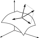
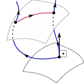
There is, however, one intriguing, compelling and physically informed contender. In mechanics and field theory it is natural to separate the flow locally into group dynamics and a transverse, ‘horizontal’ flow, Smale (1970); Abraham and Marsden (1978) by the ‘method of connections’, Rowley et al. (2003) illustrated in Fig. 12. The method of connections, however, does not reduce the dynamics to a lower-dimensional reduced state space ${\cal M}/G$. In contrast to the method of co-moving frames, where one defines a mean phase velocity of a relative periodic orbit, the method of connections is inherently local. The two methods coincide for relative equilibria.

The meaning of the ‘method of connections’ in classical dynamics is clearest in the work of Shapere and Wilczek: Shapere and Wilczek (1989, 2006) one can observe a swimmer (or our dancer) from a fixed slice frame, or bring her back to observe only the shape-changing dynamics, no drifting. Left to herself, she will reemerge in the same pose someplace else: that shift is called a ‘geometrical phase’, which -while accruing it is the whole point of swimming- has not played any role in our discussion of symmetry reduction. Conversely, most gauge choices in quantum field theory are covariant, and while that suffices to regularize path integrals, the method of slices says that this is no symmetry reduction at all, and it yields no insight into the geometry of nonlinear flows.

Symmetry reduction in dynamics (including classical field theories such as the Navier-Stokes equations) closely parallels the reduction of gauge symmetry in quantum field theories. There, the freedom of choosing moving frames shown in Fig. 5 is called ‘gauge freedom’ and a particular prescription for choosing a representative from each gauge orbit is called ‘gauge fixing’. Just like the slice hyperplanes of Fig. 7 may intersect a group orbit many times, a gauge fixing submanifold may not intersect a gauge orbit, or it may intersect it more than once (‘Gribov ambiguity’). Gribov (1978); Vandersickel and Zwanziger (2012) In this context a chart is called a ‘Gribov’ or ‘fundamental modular’ region and its border is called a ‘Gribov horizon’ (a convex manifold in the space of gauge fields). The Gribov region is compact and bounded by the Gribov horizon. Within a Gribov region the ‘Faddeev-Popov operator’ (analogue of the group orbit tangent vector) is strictly positive, while on the Gribov horizon it has at least one vanishing eigenvalue.

VII Conclusions

As turbulent flow evolves, every so often we catch a glimpse of a familiar structure. For any finite spatial resolution and time, the flow follows unstable coherent structures belonging to an alphabet of representative states, here called ‘templates’. However, in the presence of symmetries, near recurrences can be identified only if shifted both in time and space.

In the method of sections (along time direction) and slices (along spatial symmetry directions), the identification of physically nearby states is achieved by cutting group orbits with a finite set of hyperplanes, one for each continuous parameter, with each time trajectory and group orbit of symmetry-equivalent points represented by a single point. The method of slices is akin to (but distinct from) cutting across trajectories by means of sections. Both methods reduce continuous symmetries: one sections the continuous-time trajectories, the other slices the layers of the onion formed by group-orbits. Both are triggered by analogous conditions: oriented piercing of the section and oriented piercing of the slice. Just as a Poincaré section goes bad, the slice hyperplane goes bad the moment transversality is lost. A slice, however, is emphatically not a Poincaré section: as the first step in a reduction of dynamics, a slice replaces a trajectory by a continuous symmetry-reduced trajectory, whereas in the next step a Poincaré section replaces a continuous time trajectory by a discrete sequence of points.

The main lesson of the visual tour undertaken above is that if a dynamical problem has a continuous symmetry, the symmetry must be reduced before any detailed analysis of the flow’s state space geometry can take place. So far, this has only been achieved for transitionally turbulent numerical pipe flows, Willis, Cvitanović, and Avila (2012) resulting in the discovery of the first relative periodic orbits embedded in turbulence. In the future, it should be the first step in the analysis of any turbulent data, numerical or experimental. Once symmetry reduction is achieved, all solutions of a turbulent flow can be plotted together: all symmetry-equivalent states are represented by a single point, families of solutions are mapped to a single solution, relative equilibria become equilibria, relative periodic orbits become periodic orbits, and most importantly, the analysis of the global dynamical system in terms of invariant solutions and their stable/unstable manifolds can now commence.