Structural robustness and transport efficiency of complex networks with degree correlation

Abstract

We examine two properties of complex networks, the robustness against targeted node removal (attack) and the transport efficiency in terms of degree correlation in node connection by numerical evaluation of exact analytic expressions. We find that, while the assortative correlation enhances the structural robustness against attack, the disassortative correlation significantly improves the transport efficiency of the network under consideration. This finding might shed light on the reason why some networks in the real world prefer assortative correlation and others prefer disassortative one.

I Introduction

Many complex systems in the real world can be modeled by complex networks Watts and Strogatz (1998); Barabási and Albert (1999); Albert and Barabási (2002); Newman (2003); Dorogovtsev and Mendes (2003); Cohen et al. (2005); Boccaletti et al. (2006); Calderelli and Vespignani (2007); Newman (2010); Cohen and Havlin (2010); Gao et al. (2011). The cooperative performance of such complex systems relies on the global connectivity of their components. These complex systems are placed, however, in an external environment, where the components or connections could be removed and/or altered. The analysis of the response of the global connectivity caused by intentional node removal of the network, or targeted attacks, has been, therefore, one of the main issues of the complex network analysis Molloy and Reed (1995); Albert et al. (2000); Cohen et al. (2000); Moore and Newman (2000); Callaway et al. (2000); Cohen et al. (2001, 2002); Chung and Lu (2002); Schwartz et al. (2002); Gallos et al. (2005); Shargel et al. (2003); Vázquez and Moreno (2003); Paul et al. (2004); Tanizawa et al. (2005, 2006); Paul et al. (2006); Donetti et al. (2006); Paul et al. (2007); Buldyrev et al. (2010); Huang et al. (2011); Dorogovtsev and Mendes (2003); Cohen et al. (2005); Boccaletti et al. (2006); Calderelli and Vespignani (2007); Newman (2010); Cohen and Havlin (2010); Gao et al. (2011).

Although most of the existing theoretical studies on robustness analysis of complex networks are based on arguments based only on the degree distribution, the effects of degree correlation between node connection begin to be considered recently Serrano et al. (2006); Goltsev et al. (2008); Shiraki and Kabashima (2010); Ostilli et al. (2011); Tanizawa et al. (2012). In the early stage of complex network research, however, Newman already argued that networks in the real world exhibit rather strong tendency, or correlation, in the connection between nodes of different degrees Newman (2002). He introduced the terms, assortative and disassortative correlations, to describe the tendency of nodes in a network to make connections between the same degree and between different degrees, respectively. Social networks, such as friendship relations, collaboration networks in scientific research, and so on, tend to be assortative, and communication networks, such as WWW, neural networks, autonomous system networks on the Internet, and so on, tend to be disassortative. Newman also calculated the giant component collapse for specific kinds of correlated networks against random node removal and found that assortativity enhances the robustness of networks against random attack. Goltsev et al. focused on the evaluation of critical exponents of correlated complex networks in the vicinity of node percolation transition for the case of random attack Goltsev et al. (2008).

Regarding to a robustness analysis against targeted attack, Schneider et al. numerically found that the final robust network structure have a common “onion-like” topology consisting of a core of highly connected nodes hierarchically surrounded by rings of nodes with decreasing degree Schneider et al. (2011); Herrmann et al. (2011). In each ring most of the nodes are of the same degree. Tanizawa et al. took an analytic approach to the robustness analysis against targeted attack Tanizawa et al. (2012). Interestingly, they found that the optimal structure against simultaneous random and targeted attack is very similar to the “onion-like” structure found by Schneider et al. The optimal structure obtained consists of hierarchically and weakly interconnected random regular graphs and exhibits extremely assortative degree correlation.

With respect to the structural robustness against targeted attack, assortative degree correlation is favorable. However, there are considerable number of functional complex networks in the real world that show disassortative degree correlation, such as WWW, neural networks, autonomous system networks on the Internet. Within the author’s knowledge, there seems to be no plausible argument for the emergence of disassortative networks. When we consider that most of the networks that exhibit disassortativity are communication oriented, in other words, that the primary function of these networks is information exchange, it is likely that the efficiency of the information exchange dominates in determining their network structure. Gallos et al. considered the effects of degree correlation in terms of fractality in network structure and argued the particle diffusion is accelerated on the network structure with strong hub repulsion Gallos et al. (2008).

In this paper, we examine the robustness against targeted attack and the transport efficiency of complex networks in terms of assortative (disassortative) degree correlation by numerical evaluation of exact analytic expressions, expecting that the results shed some light on the reason of the emergence of assortativity (disassortativity) in various complex networks in the real world.

This paper is organized as follows. In Sec. II, we describe the theoretical framework for the calculation of the robustness and the transport efficiency of complex networks with degree correlation under the condition of fixed degree distribution. In Sec. III, we show the results of the calculation based on the theory described in Sec. II. There we see that the disassortativity enhances the transport efficiency, while the assortativity enhances the structural robustness against targeted attack. Section IV is for discussion and summary.

II Theory

II.1 Degree distribution and degree correlation

Since we consider the degree correlation in node connection, we start from the joint degree matrix, $P(k,q)$, which is the probability that a randomly chosen edge from a $k$-degree node leads to a $q$-degree node. For undirected networks, the symmetry $P(k,q)=P(q,k)$ holds. The sum of $P(k,q)$ over $q$ is the probability that a randomly chosen edge emanates from a $k$-degree node and is related to the degree distribution, $P(k)$, with the normalization condition, $\sum_{k}P(k)=1$, through the relation, $\sum_{q}P(k,q)=kP(k)/\langle k\rangle$, where $\langle k\rangle=\sum_{k}kP(k)$ is the average degree. By definition, $\sum_{k,q}P(k,q)=1$. If we fix the degree distribution, $P(k)$, the sum, $\sum_{q}P(k,q)$, has also to be fixed.

The conditional probability, $P(q|k)$, that a randomly chosen edge from a $k$-degree node leads to a $q$-degree node, which is defined by $P(q|k)\equiv P(k,q)/\sum_{q}P(k,q)=P(k,q)/\left(kP(k)/\langle k\rangle\right)$, contains the information of the degree correlation of the network under consideration. This conditional probability, $P(q|k)$, is normalized for each $k$ as $\sum_{q}P(q|k)=1$. For networks without degree correlation, $P(q|k)$ is independent of $k$ and equals to $qP(q)/\langle k\rangle$. This means that the joint degree matrix for uncorrelated networks is separable and becomes $P(k,q)=\left(kP(k)/\langle k\rangle\right)\left(qP(q)/\langle k\rangle\right)$.

Although the theoretical framework taken in this paper is generic and applicable to any form of joint degree matrices, $P(k,q)$, we here consider the cases of scale-free networks where the degree distribution takes a power-law form, $P(k)\propto k^{-\lambda}\;\left(k=m,m+1,\dots,K-1,K\right)$. Here we denote the minimum degree as $m$ and the maximum degree as $K$. In these cases, the joint degree matrix is finite and the degree dependence of its matrix elements for uncorrelated (scale-free) networks is represented by $P_{0}(k,q)\sim k^{1-\lambda}q^{1-\lambda}$. By modifying the degree dependence of the joint degree matrix from this uncorrelated one, we can introduce the degree correlation. Note that, because of the symmetry of $P(k,q)$ in terms of $k$ and $q$, we are only allowed to determine the degree dependence of $P(k,q)$ for the elements corresponding to $q\geq k$. The matrix elements for $q<k$ are determined from the symmetry and the normalization condition of $P(k,q)$.

If $P(k,q)$ decreases slower than $P_{0}(k,q)$ as $q$ increases, the tendency of nodes to make connection with nodes of larger degree is enhanced. In this case, nodes are likely to be connected to large degree nodes ($q\gg k$). Thus the correlation is disassortative. In contrast, if $P(k,q)$ decreases faster than $P_{0}(k,q)$ as $q$ increases, the tendency of nodes to make connection with nodes of larger degrees becomes smaller. In this case, nodes are more likely to be connected to nodes of similar degrees ($q\approx k$). Thus the correlation is assortative.

There are many possibilities to introduce degree correlation. Here we adopt a simple modification of the joint degree matrix, which is

$$P(k,q)\sim k^{1-\lambda}q^{1-\lambda+\epsilon}\;\;\;\left(q\geq k\right).$$ (1)

This modification leads to the conditional probability in the form

$$P(q|k)\sim q^{1-\lambda+\epsilon}\;\;\;\left(q\geq k\right).$$ (2)

In this modification the degree correlation is controlled by a single parameter $\epsilon$, which makes analysis sufficiently simple and mathematically tractable. Since $\epsilon=0$ means the absence of degree correlation, nonzero values of $\epsilon$ indicate the existence of degree correlation. For $\epsilon>0$, the values of $P(q|k)$ for larger $q$’s increase from the values of the uncorrelated networks ($\epsilon=0$), which implies that the tendency of small degree nodes making connections with large degree nodes is enhanced. Thus $\epsilon>0$ represents disassortative degree correlation. Similarly, $\epsilon<0$ represents assortative degree correlation.

II.2 Giant component collapse due to attack

In targeted attack, where the nodes of a network are removed according to the degree of nodes, the remaining fraction of $k$-degree nodes is reduced to a factor $b_{k}\>(0\leq b_{k}\leq 1)$ from the original fraction, $P(k)$. The total remaining fraction of nodes, $p$, is calculated as $p=\sum_{k}b_{k}P(k)$.

The giant component in a complex network is the largest cluster of connected nodes, where its normalized size in the network, $S$, remains finite as the total number of nodes, $N$, becomes infinite. Non-zero values of $S$ indicate a macroscopic connectivity of the network under consideration. The resiliency of $S$ under attack is taken to be a measure of the robustness of the network.

To calculate the giant component fraction, $S$, under degree correlation, we take the generating function formalism Callaway et al. (2000); Goltsev et al. (2008); Tanizawa et al. (2012). Let $x_{k}$ be the probability that a randomly chosen link from a $k$-degree node does not lead to the giant component. In the limit of $N\to\infty$, the probability that a node is connected to any node that has already been connected to other nodes is negligible, since it is proportional to some negative power of $N$. Under the condition that the network only consists of trees, the probabilities, $x_{k}\;\left(k=m,m+1,\dots,K\right)$, for non-zero values of $b_{k}$, and the node fraction of the giant component, $S$, are determined by the following set of equations:

$$x_{k} =1-\sum_{q}b_{q}P(q|k)+\sum_{q}b_{q}P(q|k)\left(x_{q}\right)^{q-1}$$ (3)

$$S =p-\sum_{k}b_{k}P(k)\left(x_{k}\right)^{k}=\sum_{k}b_{k}P(k)\left(1-(x_{k})^{k}\right).$$ (4)

Obviously, $x_{k}=1$, if all $k$-degree nodes are removed ($b_{k}=0$). The degree correlation is included in the conditional probability, $P(q|k)$. Although Eqs.  (3) and (4) contain $b_{k}$ and can be applicable to any types of degree based node removal, we focus on two simple types of attack in this paper: (i) targeted attack, which is the selective removal of nodes from the largest degree, and (ii) random attack, which is the uniform removal of nodes with equal probability.

II.3 Diffusion on correlated networks

To investigate the transport property on complex networks with degree correlation, we consider a simple diffusion process described by the following simple diffusion equation:

$$\frac{d}{dt}\rho_{k}(t)=-\rho_{k}(t)+k\sum_{q}P(q|k)\frac{\rho_{q}(t)}{q},$$ (5)

where $\rho_{k}(t)$ is the density of “particles” on a randomly selected $k$-degree node at time $t$.

The first term in the right hand side of Eq. (5) represents the diffusion from the selected $k$-degree node and the second term represents the total in-coming flow from the $q$-degree neighbor nodes through its $k$ edges. We assume that the “particles” flow out of a $k$-degree node through all of its edges with equal probability.

By taking vector notation as $\bm{\rho}(t)=\left\{\rho_{m}(t),\rho_{m+1}(t),\dots,\rho_{K-1}(t),\rho_{K}(t)\right\}$ and introducing the conditional probability matrix, $\mathsf{C}=\left\{\mathsf{C}_{kq}\right\}=kP(q|k)/q$, Eq. (5) can be simply represented as

$$\frac{d}{dt}\bm{\rho}(t)=-\left(\mathsf{I}-\mathsf{C}\right)\bm{\rho}(t),$$ (6)

where $\mathsf{I}$ is the identity matrix. By the standard diagonalization procedure, the diffusion equations for each degree are reorganized to form a set of decoupled independent diffusion equations for each diffusive “mode”. The eigenvalues of the matrix $\mathsf{I}-\mathsf{C}$, which are all non negative in the calculation presented in this paper, can be interpreted as the diffusion constants for these diffusive modes. The inverse of the largest positive eigenvalue, which we denote as $\mu$, is the smallest characteristic time, $T=1/\mu$, for these diffusive modes and serves as a good measure for evaluating the efficiency of the diffusion. Small values of $T$ imply that particles on nodes diffuse in short time intervals, which we interpret as transport efficiency of the network under consideration.

III Results

In this section, we present the results of calculation based on the theory described in the previous section for scale-free networks with the minimum degree $m=2$, the maximum degree $K=20$, and the exponent in the degree distribution, $\lambda=1.0$.

III.1 Giant component collapse

The existence of the giant component implies that the global connectivity in a network is maintained. As the total remaining node fraction, $p$, decreases, the node fraction belonging to the giant component, $S$, also decreases. Vanishing $S$ means that the global connectivity is lost and a network is disintegrated. It is well known that $S$ vanishes at a certain value of $p$, the threshold, by percolation phase transition. The value of the threshold depends on the structure of the network and the way of node removal.

For targeted attack, the parameters $b_{k}$ in Eqs. (3) and (4) are taken to be

$$b_{k}=\begin{cases}1&(m\leq k<\tilde{K}),\\ b&(k=\tilde{K}),\\ 0&(\tilde{K}<k\leq K),\end{cases}$$ (7)

where $\tilde{K}$ is the maximum degree of partially remaining nodes. The values of $\tilde{K}$ and $b$ are determined by the total remaining node fraction through $p=\sum_{k=m}^{\tilde{K}}b_{k}P(k)$. For random attack, the node removal is uniform and all $b_{k}$’s are equal to the total remaining node fraction, $p$.

Figure 1: (Color online) Plots of the giant component fraction, $S$, as a function of remaining node fraction, $p$, for scale-free networks with $m=2$, $K=20$, and $\lambda=1.0$ that have different values of $\epsilon$ from $\epsilon=-1.0$ (assortative, in blue) to $\epsilon=0.4$ (disassortative, in red) through $\epsilon=0$ (no correlation, in black). The plot (a) shows the giant component collapse due to targeted attack and the plot (b) shows the giant component collapse due to random attack. Note that, while the degree correlation plays no role in the case of random attack, the assortative (disassortative) degree correlation enhances (reduces) the resiliency of the giant component.

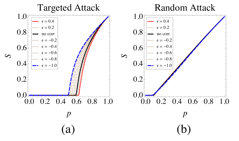
In Fig. 1, we plot the giant component fraction $S$ of scale-free networks with $m=2$, $K=20$, and $\lambda=1.0$ as a function of the remaining node fraction, $p$, for various values of $\epsilon$ from $\epsilon=-1.0$ (assortative) to $\epsilon=0.4$ (disassortative) through $\epsilon=0$ (no correlation) against targeted attack and random attack. We see from Fig. 1 (b) that the degree correlation plays almost no role in random attack. In contrast, the degree correlation significantly affects the decrease of $S$ against targeted attack (Fig. 1 (a)). As the assortativity becomes stronger ($\epsilon<0$), the steep drop in $S$ takes place at smaller values of $p$. Introducing assortative degree correlation thus makes a network more resilient against targeted attack.

Figure 2: (Color online) Plot of the robustness measure, $R$, defined in the inset of the plot and calculated from the plot, Fig. 1 (a) as a function of $\epsilon$. As the value of $\epsilon$ increases from $-1.0$ (assortative) to $0.4$ (disassortative), the robustness measure, $R$, decreases almost linearly, which implies the scale-free network becomes more vulnerable against targeted attack as the degree correlation tends to disassortative.

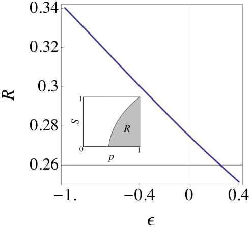
As discussed in Schneider et al. (2011); Herrmann et al. (2011); Tanizawa et al. (2012), the giant component begins to collapse faster for random attack as the assortativity sets in, while the remaining node threshold decreases slightly with the increase of assortativity. Therefore, the remaining node threshold does not serve as a good measure for the robustness. To compare the robustness against attack in terms of degree correlation, we take the area under the decreasing curve of $S$ as the robustness measure, which represents the resiliency of the giant component due to node removal much more properly. (See the inset of Fig. 2.) We plot the robustness measure, $R$, calculated from the curves of $S$ against targeted attack as a function of $\epsilon$ in Fig. 2. As the value of $\epsilon$ increases from $-1.0$ (assortative) to $0.4$ (disassortative), the robustness measure, $R$, decreases almost linearly, which implies the scale-free network becomes more vulnerable against targeted attack as the degree correlation tends to disassortative. If the robustness against targeted attack is the first priority in designing network structure, the degree correlation should be assortative.

III.2 Transport efficiency

Networks in the real world are not static objects. There are flows of material, energy, information on the networks. The transport efficiency of these flows, as well as the structural robustness, should also be one of the crucial functionalities of complex networks.

To draw an overall picture of transport efficiency with respect to degree correlation, we examine the simple diffusion equation, Eq. (5), described in the previous section.

Figure 3: (Color online) Plots of the time dependence of the density of diffusing particles on (a) a node of the minimum degree, $m$, and (b) a node of the maximum degree, $K$, in scale-free networks with $m=2$, $K=20$, and $\lambda=1.0$ according to the diffusion equation, Eq. (6), under the initial condition that all particles are uniformly distributed on nodes of the minimum degree. Thus the particles diffuse from the smallest degree nodes to all the other larger degree nodes up to the maximum degree. Note that particles diffuse faster as the correlation parameter $\epsilon$ increases from $-1.0$ (assortative, in blue) to $0.4$ (disassortative, in red).

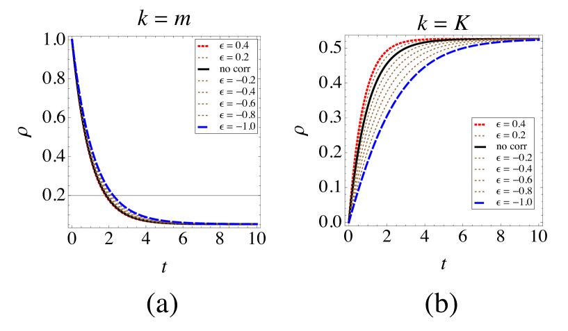
In Fig. 3, we plot the densities of diffusing particles on a node of the minimum degree and a node of the maximum degree in scale-free networks with $m=2$, $K=20$, and $\lambda=1.0$ as a function of time, $t$. In this calculation, all the particles are uniformly distributed on the nodes of minimum degree. Thus the particles flow out of minimum degree nodes and diffuse to other nodes of larger degree. Figure 3 (b) shows the increase of the density on a node of maximum degree. From this plot, we can see that the density reaches its maximum faster as the degree correlation becomes disassortative. This is because, in disassortative networks, the tendency of minimum degree nodes making connection to the maximum degree nodes is larger and that the particles on minimum degree nodes can easily diffuse to larger degree nodes through these connections.

Figure 4: (Color online) Plots of the time dependence of the density of diffusing particles on (a) a node of the minimum degree, $m$, and (b) a node of the maximum degree, $K$, in scale-free networks with $m=2$, $K=20$, and $\lambda=1.0$ according to the diffusion equation, Eq. (6), under the initial condition that all particles are uniformly distributed on nodes of the maximum degree. Thus the particles diffuse from the largest degree nodes to all the other smaller degree nodes down to the minimum degree. Note that particles diffuse faster as the correlation parameter $\epsilon$ increases from $-1.0$ (assortative, in blue) to $0.4$ (disassortative, in red).

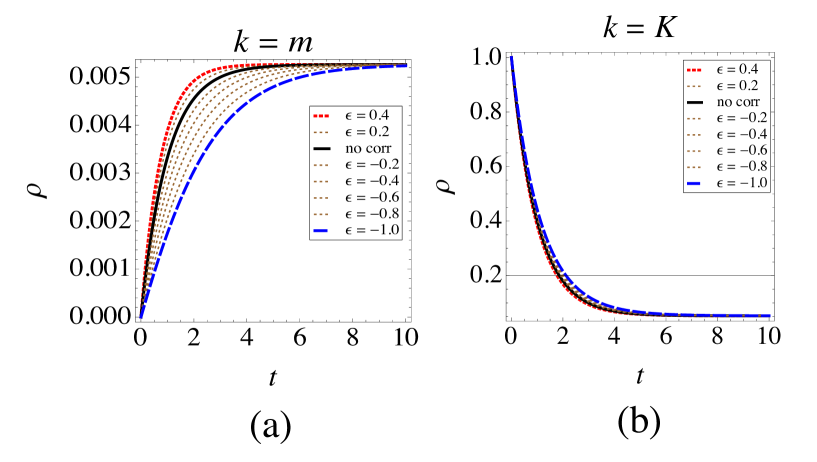
In Fig. 4, we plot the same diffusion process except for the initial condition, in which all particles are uniformly distributed on nodes of maximum degree. Also in this case, the particles diffuse faster in disassortative networks.

Figure 5: (Color online) Plot of the characteristic time for diffusion, $T$, defined by the inverse of the largest positive eigenvalue, $\mu$, of the coefficient matrix, $\mathsf{I}-\mathsf{C}$. As the value of $\epsilon$ increases from $-1.0$ (assortative) to $0.4$ (disassortative), the characteristic time, $T$, decreases almost linearly with a bend at $\left(\epsilon,T\right)=\left(0,1\right)$ (no correlation). The decreasing rate in $T$ is much steeper in the disassortative region ($\epsilon>0$) than that in the assortative region ($\epsilon<0$).

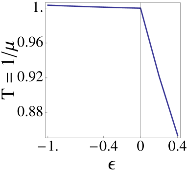
The inverse of the largest positive eigenvalues, $\mu$, of the coefficient matrix, $\mathsf{I}-\mathsf{C}$, of the diffusion equation, Eq. (6), can be taken as a measure the characteristic diffusion time, $T(=1/\mu)$, the behavior of which we plot in Fig. 5 as a function of $\epsilon$. It is interesting that the decrease in $T$ has a bend at $\left(\epsilon,T\right)=\left(0,1\right)$ (no correlation) and gets steeper in disassortative region ($\epsilon>0$). This means that the diffusion takes place much faster in disassortative networks. Thus the transport efficiency favors disassortative degree correlation.

IV Discussion and summary

Structural robustness and transport efficiency are both important qualities for the proper functioning of a complex network in the real world. From the results presented in this paper, we see that assortative correlation is favorable for structural robustness, whereas disassortative correlation is favorable for transport efficiency.

As Newman pointed out, both assortative and disassortative scale-free networks occur in the real worldNewman (2002). Social networks, such as friendship relations, collaboration networks in scientific research, and so on, tend to be assortative, and communication networks, such as WWW, neural networks, autonomous system networks on the Internet, and so on, tend to be disassortative.

Within the author’s knowledge, there is no plausible argument for the emergence of this difference. According to the results obtained here, one possible argument might be the following. If the required time scale of transport on a network for proper functioning is not so fast and the structural robustness against several types of attack is the first priority, the resulting network favors assortative degree correlation. In contrast, the transport efficiency is crucial and mandatory, the resulting network favors disassortative degree correlation. The existing examples we have at present seem to fit this reasoning.

The results presented in this paper is, however, obtained from an application of the theory to very limited cases. To confirm the validity of the argument about the emergence of degree correlation, we need more extensive and thorough investigation, which will be open to our future work.

In summary, we examine the effect of degree correlation on structural robustness and transport efficiency of scale-free networks by numerical calculation based on exact analytic equations. The transport efficiency is significantly enhanced when the degree correlation becomes disassortative, whereas the structural robustness against targeted attack is improved as the assortative degree correlation becomes stronger. These opposite roles of degree correlation played in structural robustness and transport efficiency possibly provide a plausible argument for the emergence of various degree correlation in complex networks in the real world.