The Lasso for High-Dimensional Regression with a Possible Change-Point

Abstract.

We consider a high-dimensional regression model with a possible change-point due to a covariate threshold and develop the Lasso estimator of regression coefficients as well as the threshold parameter. Our Lasso estimator not only selects covariates but also selects a model between linear and threshold regression models. Under a sparsity assumption, we derive non-asymptotic oracle inequalities for both the prediction risk and the $\ell_{1}$ estimation loss for regression coefficients. Since the Lasso estimator selects variables simultaneously, we show that oracle inequalities can be established without pretesting the existence of the threshold effect. Furthermore, we establish conditions under which the estimation error of the unknown threshold parameter can be bounded by a nearly $n^{-1}$ factor even when the number of regressors can be much larger than the sample size ($n$). We illustrate the usefulness of our proposed estimation method via Monte Carlo simulations and an application to real data.

Key words. Lasso, oracle inequalities, sample splitting, sparsity, threshold models.

1. Introduction

The Lasso and related methods have received rapidly increasing attention in statistics since the seminal work of Tibshirani (1996). For example, see a timely monograph by Bühlmann and van de Geer (2011) as well as review articles by Fan and Lv (2010) and Tibshirani (2011) for general overview and recent developments.

In this paper, we develop a method for estimating a high-dimensional regression model with a possible change-point due to a covariate threshold, while selecting relevant regressors from a set of many potential covariates. In particular, we propose the $\ell_{1}$ penalized least squares (Lasso) estimator of parameters, including the unknown threshold parameter, and analyze its properties under a sparsity assumption when the number of possible covariates can be much larger than the sample size.

To be specific, let $\{(Y_{i},X_{i},Q_{i}):i=1,\ldots,n\}$ be a sample of independent observations such that

(1.1) $$Y_{i}=X_{i}^{\prime}\beta_{0}+X_{i}^{\prime}\delta_{0}1\{Q_{i}<\tau_{0}\}+U_{i},\ \ \ i=1,\ldots,n,$$

where for each $i$, $X_{i}$ is an $M\times 1$ deterministic vector, $Q_{i}$ is a deterministic scalar, $U_{i}$ follows $N(0,\sigma^{2})$, and $1\{\cdot\}$ denotes the indicator function. The scalar variable $Q_{i}$ is the threshold variable and $\tau_{0}$ is the unknown threshold parameter. Note that since $Q_{i}$ is a fixed variable in our setup, (1.1) includes a regression model with a change-point at unknown time (e.g. $Q_{i}=i/n$). Note that in this paper, we focus on the fixed design for $\{(X_{i},Q_{i}):i=1,\ldots,n\}$ and independent normal errors $\{U_{i}:i=1,\ldots,n\}$. This setup has been extensively used in the literature (e.g. Bickel et al., 2009).

A regression model such as (1.1) offers applied researchers a simple yet useful framework to model nonlinear relationships by splitting the data into subsamples. Empirical examples include cross-country growth models with multiple equilibria (Durlauf and Johnson, 1995), racial segregation (Card et al., 2008), and financial contagion (Pesaran and Pick, 2007), among many others. Typically, the choice of the threshold variable is well motivated in applied work (e.g. initial per capita output in Durlauf and Johnson (1995), and the minority share in a neighborhood in Card et al. (2008)), but selection of other covariates is subject to applied researchers’ discretion.

However, covariate selection is important in identifying threshold effects (i.e., nonzero $\delta_{0}$) since a statistical model favoring threshold effects with a particular set of covariates could be overturned by a linear model with a broader set of regressors. Therefore, it seems natural to consider Lasso as a tool to estimate (1.1).

The statistical problem we consider is to estimate unknown parameters $(\beta_{0},\delta_{0},\tau_{0})\in\mathbb{R}^{2M+1}$ when $M$ is much larger than $n$. For the classical setup (estimation of parameters without covariate selection when $M$ is smaller than $n$), estimation of (1.1) has been well studied (e.g. Tong, 1990; Chan, 1993; Hansen, 2000). Also, a general method for testing threshold effects in regression (i.e. testing $H_{0}:\delta_{0}=0$ in (1.1)) is available for the classical setup (e.g. Lee et al., 2011).

Although there are many papers on Lasso type methods and also equally many papers on change points, sample splitting, and threshold models, there seem to be only a handful of papers that intersect both topics. Wu (2008) proposed an information-based criterion for carrying out change point analysis and variable selection simultaneously in linear models with a possible change point; however, the proposed method in Wu (2008) would be infeasible in a sparse high-dimensional model. In change-point models without covariates, Harchaoui and Lévy-Leduc (2008, 2010) proposed a method for estimating the location of change-points in one-dimensional piecewise constant signals observed in white noise, using a penalized least-square criterion with an $\ell_{1}$-type penalty. Zhang and Siegmund (2012) developed Bayes Information Criterion (BIC)-like criteria for determining the number of changes in the mean of multiple sequences of independent normal observations when the number of change-points can increase with the sample size. Ciuperca (2012) considered a similar estimation problem as ours, but the corresponding analysis is restricted to the case when the number of potential covariates is small.

In this paper, we consider the Lasso estimator of regression coefficients as well as the threshold parameter. Since the change-point parameter $\tau_{0}$ does not enter additively in (1.1), the resulting optimization problem in the Lasso estimation is non-convex. We overcome this problem by comparing the values of standard Lasso objective functions on a grid over the range of possible values of $\tau_{0}$.

Theoretical properties of the Lasso and related methods for high-dimensional data are examined by Fan and Peng (2004), Bunea et al. (2007), Candès and Tao (2007), Huang et al. (2008), Huang et al. (2008), Kim et al. (2008), Bickel et al. (2009), and Meinshausen and Yu (2009), among many others. Most of the papers consider quadratic objective functions and linear or nonparametric models with an additive mean zero error. There has been recent interest in extending this framework to generalized linear models (e.g. van de Geer, 2008; Fan and Lv, 2011), to quantile regression models (e.g. Belloni and Chernozhukov, 2011a; Bradic et al., 2011; Wang et al., 2012), and to hazards models (e.g. Bradic et al., 2012; Lin and Lv, 2013). We contribute to this literature by considering a regression model with a possible change-point and then deriving nonasymptotic oracle inequalities for both the prediction risk and the $\ell_{1}$ estimation loss for regression coefficients under a sparsity scenario.

Our theoretical results build on Bickel et al. (2009). Since the Lasso estimator selects variables simultaneously, we show that oracle inequalities similar to those obtained in Bickel et al. (2009) can be established without pretesting the existence of the threshold effect. In particular, when there is no threshold effect ($\delta_{0}=0$), we prove oracle inequalities that are basically equivalent to those in Bickel et al. (2009). Furthermore, when $\delta_{0}\neq 0$, we establish conditions under which the estimation error of the unknown threshold parameter can be bounded by a nearly $n^{-1}$ factor when the number of regressors can be much larger than the sample size. To achieve this, we develop some sophisticated chaining arguments and provide sufficient regularity conditions under which we prove oracle inequalities. The super-consistency result of $\widehat{\tau}$ is well known when the number of covariates is small (see, e.g. Chan, 1993; Seijo and Sen, 2011a, b). To the best of our knowledge, our paper is the first work that demonstrates the possibility of a nearly $n^{-1}$ bound in the context of sparse high-dimensional regression models with a change-point.

The remainder of this paper is as follows. In Section 2 we propose the Lasso estimator, and in Section 3 we give a brief illustration of our proposed estimation method using a real-data example in economics. In Section 4 we establish the prediction consistency of our Lasso estimator. In Section 5 we establish sparsity oracle inequalities in terms of both the prediction loss and the $\ell_{1}$ estimation loss for $(\alpha_{0},\tau_{0})$, while providing low-level sufficient conditions for two possible cases of threshold effects. In Section 6 we present results of some simulation studies, and Section 7 concludes. The appendices of the papr consist of 6 sections: Appendix A provides sufficient conditions for one of our main assumptions, Appendix B gives some additional discussions on identifiability for $\tau_{0}$, Appendices C, D, and E contain all the proofs, and Appendix F provides additional numerical results.

Notation

We collect the notation used in the paper here. For $\{(Y_{i},X_{i},Q_{i}):i=1,\ldots,n\}$ following (1.1), let $\mathbf{X}_{i}(\tau)$ denote the $(2M\times 1)$ vector such that $\mathbf{X}_{i}(\tau)=(X_{i}^{\prime},X_{i}^{\prime}1\{Q_{i}<\tau\})^{\prime}$ and let $\mathbf{X}(\tau)$ denote the $(n\times 2M)$ matrix whose $i$-th row is $\mathbf{X}_{i}(\tau)^{\prime}$. For an $L$-dimensional vector $a,$ let $|a|_{p}$ denote the $\ell_{p}$ norm of $a,$ and $|J(a)|$ denote the cardinality of $J(a)$, where $J(a)=\{j\in\{1,\ldots,L\}:a_{j}\neq 0\}$. In addition, let $\mathcal{M}(a)$ denote the number of nonzero elements of $a$, i.e. $\mathcal{M}(a)=\sum_{j=1}^{L}1\{a_{j}\neq 0\}=|J(a)|$. Let $a_{J}$ denote the vector in $\mathbb{R}^{L}$ that has the same coordinates as $a$ on $J$ and zero coordinates on the complement $J^{c}$ of $J$. For any $n$-dimensional vector $W=(W_{1},\ldots,W_{n})^{\prime}$, define the empirical norm as $\left\|W\right\|_{n}:=\left(n^{-1}\sum_{i=1}^{n}W_{i}^{2}\right)^{1/2}$. Let the superscript ^(j) denote the $j$-th element of a vector or the $j$-th column of a matrix depending on the context. Finally, define $f_{(\alpha,\tau)}(x,q):=x^{\prime}\beta+x^{\prime}\delta 1\{q<\tau\}$, $f_{0}(x,q):=x^{\prime}\beta_{0}+x^{\prime}\delta_{0}1\{q<\tau_{0}\}$, and $\widehat{f}(x,q):=x^{\prime}\widehat{\beta}+x^{\prime}\widehat{\delta}1\{q<\widehat{\tau}\}$. Then, we define the prediction risk as $\left\|\widehat{f}-f_{0}\right\|_{n}:=\left(\frac{1}{n}\sum_{i=1}^{n}\left(\widehat{f}(X_{i},Q_{i})-f_{0}(X_{i},Q_{i})\right)^{2}\right)^{1/2}.$

2. Lasso Estimation

Let $\alpha_{0}=(\beta_{0}^{\prime},\delta_{0}^{\prime})^{\prime}$. Then, using notation defined above, we can rewrite (1.1) as

(2.1) $$Y_{i}=\mathbf{X}_{i}(\tau_{0})^{\prime}\alpha_{0}+U_{i},\ \ \ i=1,\ldots,n.$$

Let $\mathbf{y}\equiv(Y_{1},\ldots,Y_{n})^{\prime}$. For any fixed $\tau\in\mathbb{T}$, where $\mathbb{T}\equiv[t_{0},t_{1}]$ is a parameter space for $\tau_{0}$, consider the residual sum of squares

$$S_{n}(\alpha,\tau) =n^{-1}\sum_{i=1}^{n}\left(Y_{i}-X_{i}^{\prime}\beta-X_{i}^{\prime}\delta 1\{Q_{i}<\tau\}\right)^{2}$$

$$=\left\|\mathbf{y}-\mathbf{X}(\tau)\alpha\right\|_{n}^{2},$$

where $\alpha=(\beta^{\prime},\delta^{\prime})^{\prime}$.

We define the following $(2M\times 2M)$ diagonal matrix:

$$\mathbf{D}(\tau):=\text{diag}\left\{\left\|\mathbf{X}^{(j)}(\tau)\right\|_{n},\ \ j=1,...,2M\right\}.$$

For each fixed $\tau\in\mathbb{T}$, define the Lasso solution $\widehat{\alpha}(\tau)$ by

(2.2) $$\widehat{\alpha}(\tau):=\text{argmin}_{\alpha\in\mathcal{A}\subset\mathbb{R}^{2M}}\left\{S_{n}(\alpha,\tau)+\lambda\left|\mathbf{D}(\tau)\alpha\right|_{1}\right\},$$

where $\lambda$ is a tuning parameter that depends on $n$ and $\mathcal{A}$ is a parameter space for $\alpha_{0}$.

It is important to note that the scale-normalizing factor $\mathbf{D}(\tau)$ depends on $\tau$ since different values of $\tau$ generate different dictionaries $\mathbf{X}(\tau)$. To see more clearly, define

(2.3) $$\begin{split}X^{\left(j\right)}&\equiv(X_{1}^{(j)},\ldots,X_{n}^{(j)})^{\prime},\\ X^{\left(j\right)}(\tau)&\equiv(X_{1}^{(j)}1\{Q_{1}<\tau\},\ldots,X_{n}^{(j)}1\{Q_{n}<\tau\})^{\prime}.\end{split}$$

Then, for each $\tau\in\mathbb{T}$ and for each $j=1,\ldots,M$, we have $\left\|\mathbf{X}^{(j)}(\tau)\right\|_{n}=\left\|X^{\left(j\right)}\right\|_{n}$ and $\left\|\mathbf{X}^{(M+j)}(\tau)\right\|_{n}=\left\|X^{\left(j\right)}(\tau)\right\|_{n}$. Using this notation, we rewrite the $\ell_{1}$ penalty as

$$\lambda\left|\mathbf{D}(\tau)\alpha\right|_{1} =\lambda\sum_{j=1}^{2M}\left\|\mathbf{X}^{(j)}(\tau)\right\|_{n}\left|\alpha^{(j)}\right|$$

$$=\lambda\sum_{j=1}^{M}\left[\left\|X^{\left(j\right)}\right\|_{n}\left|\alpha^{(j)}\right|+\left\|X^{\left(j\right)}(\tau)\right\|_{n}\left|\alpha^{(M+j)}\right|\right].$$

Therefore, for each fixed $\tau\in\mathbb{T}$, $\widehat{\alpha}(\tau)$ is the weighted Lasso that uses a data-dependent $\ell_{1}$ penalty to balance covariates adequately.

We now estimate $\tau_{0}$ by

(2.4) $$\widehat{\tau}:=\text{argmin}_{\tau\in\mathbb{T}\subset\mathbb{R}}\left\{S_{n}(\widehat{\alpha}(\tau),\tau)+\lambda\left|\mathbf{D}(\tau)\widehat{\alpha}(\tau)\right|_{1}\right\}.$$

In fact, for any finite $n,$ $\widehat{\tau}$ is given by an interval and we simply define the maximum of the interval as our estimator. If we wrote the model using $1\left\{Q_{i}>\tau\right\},$ then the convention would be the minimum of the interval being the estimator. Then the estimator of $\alpha_{0}$ is defined as $\widehat{\alpha}:=\widehat{\alpha}(\widehat{\tau})$. In fact, our proposed estimator of $(\alpha,\tau)$ can be viewed as the one-step minimizer such that:

(2.5) $$(\widehat{\alpha},\widehat{\tau}):=\text{argmin}_{\alpha\in\mathcal{A}\subset\mathbb{R}^{2M},\tau\in\mathbb{T}\subset\mathbb{R}}\left\{S_{n}(\alpha,\tau)+\lambda\left|\mathbf{D}(\tau)\alpha\right|_{1}\right\}.$$

It is worth noting that we penalize $\beta_{0}$ and $\delta_{0}$ in (2.5), where $\delta_{0}$ is the change of regression coefficients between two regimes. The model in (1.1) can be written as

(2.6) $$\begin{split}Y_{i}&=X_{i}^{\prime}\beta_{0}+U_{i},\ \ \ \text{if $Q_{i}\geq\tau_{0}$},\\ Y_{i}&=X_{i}^{\prime}\beta_{1}+U_{i},\ \ \ \text{if $Q_{i}<\tau_{0}$},\end{split}$$

where $\beta_{1}\equiv\beta_{0}+\delta_{0}$. In view of (2.6), alternatively, one might penalize $\beta_{0}$ and $\beta_{1}$ instead of $\beta_{0}$ and $\delta_{0}$. We opted to penalize $\delta_{0}$ in this paper since the case of $\delta_{0}=0$ corresponds to the linear model. If $\widehat{\delta}=0$, then this case amounts to selecting the linear model.

3. Empirical Illustration

In this section, we apply the proposed Lasso method to growth regression models in economics. The neoclassical growth model predicts that economic growth rates converge in the long run. This theory has been tested empirically by looking at the negative relationship between the long-run growth rate and the initial GDP given other covariates (see Barro and Sala-i-Martin (1995) and Durlauf et al. (2005) for literature reviews). Although empirical results confirmed the negative relationship between the growth rate and the initial GDP, there has been some criticism that the results depend heavily on the selection of covariates. Recently, Belloni and Chernozhukov (2011b) show that the Lasso estimation can help select the covariates in the linear growth regression model and that the Lasso estimation results reconfirm the negative relationship between the long-run growth rate and the initial GDP.

We consider the growth regression model with a possible threshold. Durlauf and Johnson (1995) provide the theoretical background of the existence of multiple steady states and estimate the model with two possible threshold variables. They check the robustness by adding other available covariates in the model, but it is not still free from the criticism of the ad hoc variable selection. Our proposed Lasso method might be a good alternative in this situation. Furthermore, as we will show later, our method works well even if there is no threshold effect in the model. Therefore, one might expect more robust results from our approach.

The regression model we consider has the following form:

(3.1) $$\mathit{gr}_{i}=\beta_{0}+\beta_{1}\mathit{lgdp60}_{i}+X_{i}^{\prime}\beta_{2}+1\{Q_{i}<\tau\}\left(\delta_{0}+\delta_{1}\mathit{lgdp60}_{i}+X_{i}^{\prime}\delta_{2}\right)+\varepsilon_{i},$$

where $\mathit{gr}_{i}$ is the annualized GDP growth rate of country $i$ from 1960 to 1985, $\mathit{lgdp60}_{i}$ is the log GDP in 1960, and $Q_{i}$ is a possible threshold variable for which we use the initial GDP or the adult literacy rate in 1960 following Durlauf and Johnson (1995). Finally, $X_{i}$ is a vector of additional covariates related to education, market efficiency, political stability, market openness, and demographic characteristics. In addition, $X_{i}$ contains cross product terms between $\mathit{lgdp60}_{i}$ and education variables. Table 1 gives the list of all covariates used and the description of each variable. We include as many covariates as possible, which might mitigate the potential omitted variable bias. The data set mostly comes from Barro and Lee (1994), and the additional adult literacy rate is from Durlauf and Johnson (1995). Because of missing observations, we have 80 observations with 46 covariates (including a constant term) when $Q_{i}$ is the initial GDP ($n=80$ and $M=46$), and 70 observations with 47 covariates when $Q_{i}$ is the literacy rate ($n=70$ and $M=47$). It is worthwhile to note that the number of covariates in the threshold models is bigger than the number of observations ($2M>n$ in our notation). Thus, we cannot adopt the standard least squares method to estimate the threshold regression model.

Table 2 summarizes the model selection and estimation results when $Q_{i}$ is the initial GDP. In Appendix F (see Table 4), we report additional empirical results with $Q_{i}$ being the literacy rate. To compare different model specifications, we also estimate a linear model, i.e. all $\delta$’s are zeros in (3.1), by the standard Lasso estimation. In each case, the regularization parameter $\lambda$ is chosen by the ‘leave-one-out’ cross validation method. For the range $\mathbb{T}$ of the threshold parameter, we consider an interval between the 10% and 90% sample quantiles for each threshold variable.

Main empirical findings are as follows. First, the marginal effect of $\mathit{lgdp60}_{i}$, which is given by

$$\frac{\partial\mathit{gr}_{i}}{\partial\mathit{lgdp60}_{i}}=\beta_{1}+\mathit{educ}_{i}^{\prime}\tilde{\beta}_{2}+1\{Q_{i}<\gamma\}(\delta_{1}+\mathit{educ}_{i}^{\prime}\tilde{\delta}_{2}),$$

where $\mathit{educ}_{i}$ is a vector of education variables and $\tilde{\beta}_{2}$ and $\tilde{\delta}_{2}$ are sub-vectors of $\beta_{2}$ and $\delta_{2}$ corresponding to $\mathit{educ}_{i}$, is estimated to be negative for all the observed values of $\mathit{educ}_{i}$. This confirms the theory of the neoclassical growth model. Second, some non-zero coefficients of interaction terms between lgdp60 and various education variables show the existence of threshold effects in both threshold model specifications. This result implies that the growth convergence rates can vary according to different levels of the initial GDP or the adult literacy rate in 1960. Specifically, in both threshold models, we have $\delta_{1}=0$, but some $\delta_{2}$’s are not zeros. Thus, conditional on other covariates, there exist different technological diffusion effects according to the threshold point. For example, a developing country (lower $Q$) with a higher education level will converge faster perhaps by absorbing advanced technology more easily and more quickly. Finally, the Lasso with the threshold model specification selects a more parsimonious model than that with the linear specification even though the former doubles the number of potential covariates.

4. Prediction Consistency of the Lasso Estimator

In this section, we consider the prediction consistency of the Lasso estimator. We make the following assumptions.

Assumption 1.

(i) For the parameter space $\mathcal{A}$ for $\alpha_{0}$, any $\alpha\equiv(\alpha_{1},\ldots,\alpha_{2M})\in\mathcal{A}\subset\mathbb{R}^{2M}$, including $\alpha_{0}$, satisfies $\max_{j=1,\ldots,2M}\left|\alpha_{j}\right|\leq C_{1}$ for some constant $C_{1}>0$. In addition, $\tau_{0}\in\mathbb{T}\equiv[t_{0},t_{1}]$ that satisfies $\min_{i=1,\ldots,n}Q_{i}<t_{0}<t_{1}<\max_{i=1,\ldots,n}Q_{i}$. (ii) There exist universal constants $C_{2}>0$ and $C_{3}>0$ such that $\left\|\mathbf{X}^{(j)}(\tau)\right\|_{n}\leq C_{2}$ uniformly in $j$ and $\tau\in\mathbb{T}$, and $\left\|\mathbf{X}^{(j)}(t_{0})\right\|_{n}\geq C_{3}$ uniformly in $j$, where $j=1,...,2M$. (iii) There is no $i\neq j$ such that $Q_{i}=Q_{j}.$

Assumption 1(i) imposes the boundedness for each component of the parameter vector. The first part of Assumption 1(i) implies that $\left|\alpha\right|_{1}\leq 2C_{1}M$ for any $\alpha\in\mathcal{A}$, which seems to be weak, since the sparsity assumption implies that $\left|\alpha_{0}\right|_{1}$ is much smaller than $C_{1}M$. Furthermore, in the literature on change-point and threshold models, it is common to assume that the parameter space is compact. For example, see Seijo and Sen (2011a, b).

The Lasso estimator in (2.5) can be computed without knowing the value of $C_{1}$, but $\mathbb{T}\equiv[t_{0},t_{1}]$ has to be specified. In practice, researchers tend to choose some strict subset of the range of observed values of the threshold variable. Assumption 1(ii) imposes that each covariate is of the same magnitude uniformly over $\tau$. In view of the assumption that $\min_{i=1,\ldots,n}Q_{i}<t_{0}$, it is not stringent to assume that $\left\|\mathbf{X}^{(j)}(t_{0})\right\|_{n}$ is bounded away from zero.

Assumption 1(iii) imposes that there is no tie among $Q_{i}$’s. This is a convenient assumption such that we can always transform general $Q_{i}$ to $Q_{i}=i/n$ without loss of generality. This holds with probability one for the random design case if $Q_{i}$ is continuously distributed.

Define

$$r_{n}:=\min_{1\leq j\leq M}\frac{\left\|X^{\left(j\right)}(t_{0})\right\|_{n}^{2}}{\left\|X^{\left(j\right)}\right\|_{n}^{2}},$$

where $X^{\left(j\right)}$ and $X^{\left(j\right)}(\tau)$ are defined in (2.3). Assumption 1(ii) implies that $r_{n}$ is bounded away from zero. In particular, we have that $1\geq r_{n}\geq C_{3}/C_{2}>0$.

Recall that

(4.1) $$\left\|\widehat{f}-f_{0}\right\|_{n}:=\left(\frac{1}{n}\sum_{i=1}^{n}\left(\widehat{f}(X_{i},Q_{i})-f_{0}(X_{i},Q_{i})\right)^{2}\right)^{1/2}.$$

where $\widehat{f}(x,q):=x^{\prime}\widehat{\beta}+x^{\prime}\widehat{\delta}1\{q<\widehat{\tau}\}$ and $f_{0}(x,q):=x^{\prime}\beta_{0}+x^{\prime}\delta_{0}1\{q<\tau_{0}\}$. To establish theoretical results in the paper (in particular, oracle inequalities in Section 5), let $(\widehat{\alpha},\widehat{\tau})$ be the Lasso estimator defined by (2.5) with

(4.2) $$\lambda=A\sigma\Big{(}\frac{\log 3M}{nr_{n}}\Big{)}^{1/2}$$

for a constant $A>2\sqrt{2}/\mu$, where $\mu\in(0,1)$ is a fixed constant. We now present the first theoretical result of this paper.

Theorem 1 (Consistency of the Lasso).

Let Assumption 1 hold. Let $\mu$ be a constant such that $0<\mu<1$, and let $(\widehat{\alpha},\widehat{\tau})$ be the Lasso estimator defined by (2.5) with $\lambda$ given by (4.2). Then, with probability at least $1-\left(3M\right)^{1-A^{2}\mu^{2}/8}$, we have

$$\left\|\widehat{f}-f_{0}\right\|_{n} \leq K_{1}\sqrt{\lambda\mathcal{M}(\alpha_{0})},$$

where $K_{1}\equiv\sqrt{2C_{1}C_{2}(3+\mu)}>0$.

The nonasymptotic upper bound on the prediction risk in Theorem 1 can be translated easily into asymptotic convergence. Theorem 1 implies the consistency of the Lasso, provided that $n\rightarrow\infty$, $M\rightarrow\infty$, and $\lambda\mathcal{M}(\alpha_{0})\rightarrow 0$. Recall that $\mathcal{M}(\alpha_{0})$ represents the sparsity of the model (2.1). Note that in view of (4.2), the condition $\lambda\mathcal{M}(\alpha_{0})\rightarrow 0$ requires that $\mathcal{M}(\alpha_{0})=o(\sqrt{nr_{n}/\log 3M})$. This implies that $\mathcal{M}(\alpha_{0})$ can increase with $n$.

Remark 1.

Note that the prediction error increases as $A$ or $\mu$ increases; however, the probability of correct recovery increases if $A$ or $\mu$ increases. Therefore, there exists a tradeoff between the prediction error and the probability of correct recovery.

5. Oracle Inequalities

In this section, we establish finite sample sparsity oracle inequalities in terms of both the prediction loss and the $\ell_{1}$ estimation loss for unknown parameters. First of all, we make the following assumption.

Assumption 2 (Uniform Restricted Eigenvalue (URE) $(s,c_{0},\mathbb{S})$).

For some integer $s$ such that $1\leq s\leq 2M$, a positive number $c_{0}$, and some set $\mathbb{S}\subset\mathbb{R}$, the following condition holds:

$$\kappa(s,c_{0},\mathbb{S}):=\min_{\tau\in\mathbb{S}}\min_{\begin{subarray}{c}J_{0}\subseteq\{1,\ldots,2M\},\\ |J_{0}|\leq s\end{subarray}}\min_{\begin{subarray}{c}\gamma\neq 0,\\ \left|\gamma_{J_{0}^{c}}\right|_{1}\leq c_{0}\left|\gamma_{J_{0}}\right|_{1}\end{subarray}}\frac{|\mathbf{X}(\tau)\gamma|_{2}}{\sqrt{n}|\gamma_{J_{0}}|_{2}}>0.$$

If $\tau_{0}$ were known, then Assumption 2 is just a restatement of the restricted eigenvalue assumption of Bickel et al. (2009) with $\mathbb{S}=\{\tau_{0}\}$. Bickel et al. (2009) provide sufficient conditions for the restricted eigenvalue condition. In addition, van de Geer and Bühlmann (2009) show the relations between the restricted eigenvalue condition and other conditions on the design matrix, and Raskutti et al. (2010) prove that restricted eigenvalue conditions hold with high probability for a large class of correlated Gaussian design matrices.

If $\tau_{0}$ is unknown as in our setup, it seems necessary to assume that the restricted eigenvalue condition holds uniformly over $\tau$. We consider separately two cases depending on whether $\delta_{0}=0$ or not. On the one hand, if $\delta_{0}=0$ so that $\tau_{0}$ is not identifiable, then we need to assume that the URE condition holds uniformly on the whole parameter space, $\mathbb{T}$. On the other hand, if $\delta_{0}\neq 0$ so that $\tau_{0}$ is identifiable, then it suffices to impose the URE condition holds uniformly on a neighborhood of $\tau_{0}$. In Appendix A, we provide two types of sufficient conditions for Assumption 2. One type is based on modifications of Assumption 2 of Bickel et al. (2009) and the other type is in the same spirit as van de Geer and Bühlmann (2009, Section 10.1). Using the second type of results, we verify primitive sufficient conditions for the URE condition in the context of our simulation designs. See Appendix A for details.

The URE condition is useful for us to improve the result in Theorem 1. Recall that in Theorem 1, the prediction risk is bounded by a factor of $\sqrt{\lambda\mathcal{M}(\alpha_{0})}$. This bound is too large to give us an oracle inequality. We will show below that we can establish non-asymptotic oracle inequalities for the prediction risk as well as the $\ell_{1}$ estimation loss, thanks to the URE condition.

The strength of the proposed Lasso method is that it is not necessary to know or pretest whether $\delta_{0}=0$ or not. It is worth noting that we do not have to know whether there exists a threshold in the model in order to establish oracle inequalities for the prediction risk and the $\ell_{1}$ estimation loss for $\alpha_{0}$, although we divide our theoretical results into two cases below. This implies that we can make prediction and estimate $\alpha_{0}$ precisely without knowing the presence of threshold effect or without pretesting for it.

5.1. Case I. No Threshold

We first consider the case that $\delta_{0}=0$. In other words, we estimate a threshold model via the Lasso method, but the true model is simply a linear model $Y_{i}=X_{i}^{\prime}\beta_{0}+U_{i}$. This is an important case to consider in applications, because one may not be sure not only about covariates selection but also about the existence of the threshold in the model.

Let $\phi_{\max}$ denote the supremum (over $\tau\in\mathbb{T}$) of the largest eigenvalue of $\mathbf{X}(\tau)^{\prime}\mathbf{X}(\tau)/n$. Then by definition, the largest eigenvalue of $\mathbf{X}(\tau)^{\prime}\mathbf{X}(\tau)/n$ is bounded uniformly in $\tau\in\mathbb{T}$ by $\phi_{\max}$. The following theorem gives oracle inequalities for the first case.

Theorem 2.

Suppose that $\delta_{0}=0$. Let Assumptions 1 and 2 hold with $\kappa=\kappa(s,\frac{1+\mu}{1-\mu},\mathbb{T})$ for $0<\mu<1$, and $\mathcal{M}(\alpha_{0})\leq s\leq M$. Let $(\widehat{\alpha},\widehat{\tau})$ be the Lasso estimator defined by (2.5) with $\lambda$ given by (4.2). Then, with probability at least $1-\left(3M\right)^{1-A^{2}\mu^{2}/8},$ we have

$$\left\|\widehat{f}-f_{0}\right\|_{n} \leq K_{2}\frac{\sigma}{\kappa}\left(\frac{\log 3M}{nr_{n}}s\right)^{1/2},$$

$$\left|\widehat{\alpha}-\alpha_{0}\right|_{1} \leq K_{2}\frac{\sigma}{\kappa^{2}}\left(\frac{\log 3M}{nr_{n}}\right)^{1/2}s,$$

$$\mathcal{M}(\widehat{\alpha}) \leq K_{2}\frac{\phi_{\max}}{\kappa^{2}}s$$

for some universal constant $K_{2}>0$.

To appreciate the usefulness of the inequalities derived above, it is worth comparing inequalities in Theorem 2 with those in Theorem 7.2 of Bickel et al. (2009). The latter corresponds to the case that $\delta_{0}=0$ is known a priori and $\lambda=2A\sigma({\log M}/{n})^{1/2}$ using our notation. If we compare Theorem 2 with Theorem 7.2 of Bickel et al. (2009), we can see that the Lasso estimator in (2.5) gives qualitatively the same oracle inequalities as the Lasso estimator in the linear model, even though our model is much more overparametrized in that $\delta$ and $\tau$ are added to $\beta$ as parameters to estimate.

Also, as in Bickel et al. (2009), there is no requirement on $\alpha_{0}$ such that the minimum value of nonzero components of $\alpha_{0}$ is bounded away from zero. In other words, there is no need to assume the minimum strength of the signals. Furthermore, $\alpha_{0}$ is well estimated here even if $\tau_{0}$ is not identifiable at all. Finally, note that the value of the constant $K_{2}$ is given in the proof of Theorem 2 and that Theorem 2 can be translated easily into asymptotic oracle results as well, since both $\kappa$ and $r_{n}$ are bounded away from zero by the URE condition and Assumption 1, respectively.

5.2. Case II. Fixed Threshold

This subsection explores the case where the threshold effect is well-identified and discontinuous. We begin with the following additional assumptions to reflect this.

Assumption 3 (Identifiability under Sparsity and Discontinuity of Regression).

For a given $s\geq\mathcal{M}\left(\alpha_{0}\right),$ and for any $\eta$ and $\tau$ such that $\left|\tau-\tau_{0}\right|>\eta\geq\min_{i}\left|Q_{i}-\tau_{0}\right|$ and $\alpha\in\left\{\mathcal{\alpha}:\mathcal{M}\left(\alpha\right)\leq s\right\}$, there exists a constant $c>0$ such that

$$\left\|f_{\left(\alpha,\tau\right)}-f_{0}\right\|_{n}^{2}>c\eta.$$

Assumption 3 implies, among other things, that for some $s\geq\mathcal{M}\left(\alpha_{0}\right),\$and for any $\alpha\in\left\{\mathcal{\alpha}:\mathcal{M}\left(\alpha\right)\leq s\right\}$ and $\tau$ such that $\left(\alpha,\tau\right)\neq\left(\alpha_{0},\tau_{0}\right)$,

(5.1) $$\left\|f_{\left(\alpha,\tau\right)}-f_{0}\right\|_{n}\neq 0.$$

This condition can be regarded as identifiability of $\tau_{0}$. If $\tau_{0}$ were known, then a sufficient condition for the identifiability under the sparsity would be that $URE\left(s,c_{0},\{\tau_{0}\}\right)$ holds for some $c_{0}\geq 1$. Thus, the main point in (5.1) is that there is no sparse representation that is equivalent to $f_{0}$ when the sample is split by $\tau\neq\tau_{0}.$ In fact, Assumption 3 is stronger than just the identifiability of $\tau_{0}$ as it specifies the rate of deviation in $f$ as $\tau$ moves away from $\tau_{0},$ which in turn dictates the bound for the estimation error of $\widehat{\tau}$. We provide further discussions on Assumption 3 in Appendix B.

Remark 2.

The restriction $\eta\geq\min_{i}\left|Q_{i}-\tau_{0}\right|$ in Assumption 3 is necessary since we consider the fixed design for both $X_{i}$ and $Q_{i}$. Throughout this section, we implicitly assume that the sample size $n$ is large enough such that $\min_{i}\left|Q_{i}-\tau_{0}\right|$ is very small, implying that the restriction $\eta\geq\min_{i}\left|Q_{i}-\tau_{0}\right|$ never binds in any of inequalities below. This is typically true for the random design case if $Q_{i}$ is continuously distributed.

Assumption 4 (Smoothness of Design).

For any $\eta>0,$ there exists a constant $C<\infty$ such that

$$\sup_{j}\sup_{\left|\tau-\tau_{0}\right|<\eta}\frac{1}{n}\sum_{i=1}^{n}\left|X_{i}^{\left(j\right)}\right|^{2}\left|1\left(Q_{i}<\tau_{0}\right)-1\left(Q_{i}<\tau\right)\right|\leq C\eta.$$

Assumption 4 has been assumed in the classical setup with a fixed number of stochastic regressors to exclude cases like $Q_{i}$ has a point mass at $\tau_{0}\$or $\mathbb{E}\left(X_{i}|Q_{i}=\tau_{0}\right)$ is unbounded. In our setup, Assumption 4 amounts to a deterministic version of some smoothness assumption for the distribution of the threshold variable $Q_{i}$. When $(X_{i},Q_{i})$ is a random vector, it is satisfied under the standard assumption that $Q_{i}$ is continuously distributed and $\mathbb{E}(|X_{i}^{\left(j\right)}|^{2}|Q_{i}=\tau)$ is continuous and bounded in a neighborhood of $\tau_{0}$ for each $j$.

To simplify notation, in the following theorem, we assume without loss of generality that $Q_{i}=i/n$. Then $\mathbb{T}=[t_{0},t_{1}]\subset(0,1)$. In addition, let $\eta_{0}=\max\left\{n^{-1},K_{1}\sqrt{\lambda\mathcal{M}(\alpha_{0})}\right\}$, where $K_{1}$ is the same constant in Theorem 1.

Assumption 5 (Well-defined Second Moments).

For any $\eta$ such that $1/n\leq\eta\leq\eta_{0}$, $h_{n}^{2}(\eta)$ is bounded, where

$$h_{n}^{2}\left(\eta\right):=\frac{1}{2n\eta}\sum_{i=\max\{1,\left[n\left(\tau_{0}-\eta\right)\right]\}}^{\min\{\left[n\left(\tau_{0}+\eta\right)\right],n\}}\left(X_{i}^{\prime}\delta_{0}\right)^{2}$$

and $[\cdot]$ denotes an integer part of any real number.

Assumption 5 assumes that $h_{n}^{2}(\eta)$ is well defined for any $\eta$ such that $1/n\leq\eta\leq\eta_{0}$. Assumption 5 amounts to some weak regularity condition on the second moments of the fixed design. Assumption 3 implies that $\delta_{0}\neq 0$ and that $h_{n}^{2}(\eta)$ is bounded away from zero. Hence, Assumptions 3 and 5 imply that $h_{n}^{2}(\eta)$ is bounded and bounded away from zero.

To present the theorem below, it is necessary to make one additional technical assumption (see Assumption 6 in Appendix E). We opted not to show Assumption 6 here, since we believe this is just a sufficient condition that does not add much to our understanding of the main result. However, we would like to point out that Assumption 6 can hold for all sufficiently large $n$, provided that $s\lambda\left|\delta_{0}\right|_{1}\rightarrow 0$, as $n\rightarrow 0$. See Remark 4 in Appendix E for details.

We now give the main result of this section.

Theorem 3.

Suppose that Assumptions 1 and 2 hold with $\mathbb{S}=\left\{\left|\tau-\tau_{0}\right|\leq\eta_{0}\right\}$, $\kappa=\kappa(s,\frac{2+\mu}{1-\mu},\mathbb{S})$ for $0<\mu<1,$ and $\mathcal{M}(\alpha_{0})\leq s\leq M$. Furthermore, Assumptions 3, 4, and 5 hold and let $n$ be large enough so that Assumption 6 in Appendix E holds. Let $(\widehat{\alpha},\widehat{\tau})$ be the Lasso estimator defined by (2.5) with $\lambda$ given by (4.2). Then, with probability at least $1-\left(3M\right)^{1-A^{2}\mu^{2}/8}-C_{4}\left(3M\right)^{-C_{5}/r_{n}}$ for some positive constants $C_{4}$ and $C_{5}$, we have

$$\left\|\widehat{f}-f_{0}\right\|_{n} \leq K_{3}\frac{\sigma}{\kappa}\left(\frac{\log 3M}{nr_{n}}s\right)^{1/2},$$

$$\left|\widehat{\alpha}-\alpha_{0}\right|_{1} \leq K_{3}\frac{\sigma}{\kappa^{2}}\left({\frac{\log 3M}{nr_{n}}}\right)^{1/2}s,$$

$$\left|\hat{\tau}-\tau_{0}\right| \leq K_{3}\frac{\sigma^{2}}{\kappa^{2}}\frac{\log 3M}{nr_{n}}s,$$

$$\mathcal{M}\left(\hat{\alpha}\right) \leq K_{3}\frac{\phi_{\max}}{\kappa^{2}}s$$

for some universal constant $K_{3}>0$.

Theorem 3 gives the same inequalities (up to constants) as those in Theorem 2 for the prediction risk as well as the $\ell_{1}$ estimation loss for $\alpha_{0}$. It is important to note that $\left|\hat{\tau}-\tau_{0}\right|$ is bounded by a constant times $s\log 3M/(nr_{n})$, whereas $\left|\widehat{\alpha}-\alpha_{0}\right|_{1}$ is bounded by a constant times $s[\log 3M/({nr_{n}})]^{1/2}$. This can be viewed as a nonasymptotic version of the super-consistency of $\widehat{\tau}$ to $\tau_{0}$. As noted at the end of Section 5.1, since both $\kappa$ and $r_{n}$ are bounded away from zero by the URE condition and Assumption 1, respectively, Theorem 3 implies asymptotic rate results immediately. The values of constants $C_{4}$, $C_{5}$ and $K_{3}$ are given in the proof of Theorem 3.

The main contribution of this section is that we have extended the well-known super-consistency result of $\widehat{\tau}$ when $M<n$ (see, e.g. Chan, 1993; Seijo and Sen, 2011a, b) to the high-dimensional setup ($M\gg n$). In both cases, the main reason we achieve the super-consistency for the threshold parameter is that the least squares objective function behaves locally linearly around the true threshold parameter value rather than locally quadratically, as in regular estimation problems. An interesting remaining research question is to investigate whether it would be possible to obtain the super-consistency result of $\widehat{\tau}$ under a weaker condition, perhaps without a restricted eigenvalue condition.

6. Monte Carlo Experiments

In this section we conduct some simulation studies and check the properties of the proposed Lasso estimator. The baseline model is (1.1), where $X_{i}$ is an $M$-dimensional vector generated from $N(0,I)$, $Q_{i}$ is a scalar generated from the uniform distribution on the interval of $(0,1)$, and the error term $U_{i}$ is generated from $N(0,0.5^{2})$. The threshold parameter is set to $\tau_{0}=0.3,0.4,$ and $0.5$ depending on the simulation design, and the coefficients are set to $\beta_{0}=(1,0,1,0,\ldots,0)$, and $\delta_{0}=c\cdot(0,-1,1,0,\ldots,0)$ where $c=0$ or $1$. Note that there is no threshold effect when $c=0$. The number of observations is set to $n=200$. Finally, the dimension of $X_{i}$ in each design is set to $M=50,100,200$ and $400$, so that the total number of regressors are 100, 200, 400 and 800, respectively. The range of $\tau$ is $\mathbb{T}=[0.15,0.85]$.

We can estimate the parameters by the standard LASSO/LARS algorithm of Efron et al. (2004) without much modification. Given a regularization parameter value $\lambda$, we estimate the model for each grid point of $\tau$ that spans over 71 equi-spaced points on $\mathbb{T}$. This procedure can be conducted by using the standard linear Lasso. Next, we plug-in the estimated parameter $\widehat{\alpha}(\tau):=\left(\widehat{\beta}(\tau)^{\prime},\widehat{\delta}(\tau)^{\prime}\right)^{\prime}$ for each $\tau$ into the objective function and choose $\widehat{\tau}$ by (2.4). Finally, $\widehat{\alpha}$ is estimated by $\widehat{\alpha}(\widehat{\tau})$. The regularization parameter $\lambda$ is chosen by (4.2) where $\sigma=0.5$ is assumed to be known. For the constant $A$, we use four different values: $A=2.8,3.2,3.6,$ and $4.0$.

Table 3 and Figures 1–2 summarize these simulation results. To compare the performance of the Lasso estimator, we also report the estimation results of the least squares estimation (Least Squares) available only when $M=50$ and two oracle models (Oracle 1 and Oracle 2, respectively). Oracle 1 assumes that the regressors with non-zero coefficients are known. In addition to that, Oracle 2 assumes that the true threshold parameter $\tau_{0}$ is known. Thus, when $c\neq 0$, Oracle 1 estimates $(\beta^{(1)},\beta^{(3)},\delta^{(2)},\delta^{(3)})$ and $\tau$ using the least squares estimation while Oracle 2 estimates only $(\beta^{(1)},\beta^{(3)},\delta^{(2)},\delta^{(3)})$. When $c=0$, both Oracle 1 and Oracle 2 estimate only $(\beta^{(1)},\beta^{(3)})$. All results are based on 400 replications of each sample.

The reported mean-squared prediction error ($PE$) for each sample is calculated numerically as follows. For each sample $s$, we have the estimates $\widehat{\beta}_{s}$, $\widehat{\delta}_{s}$, and $\widehat{\tau}_{s}$. Given these estimates, we generate a new data $\{Y_{j},X_{j},Q_{j}\}$ of 400 observations and calculate the prediction error as

(6.1) $$\widehat{PE}_{s}=\frac{1}{400}\sum_{j=1}^{400}\left(f_{0}(x_{j},q_{j})-\widehat{f}(x_{j},q_{j})\right)^{2}.$$

The mean, median, and standard deviation of the prediction error are calculated from the 400 replications, $\{\widehat{PE}_{s}\}_{s=1}^{400}$. We also report the mean of $\mathcal{M}(\widehat{\alpha})$ and $\ell_{1}$-errors for $\alpha$ and $\tau$. Table 3 reports the simulation results of $M=50$. For simulation designs with $M>50$, Least Squares is not available, and we summarize the same statistics only for the Lasso estimation in Figures 1–2.

When $M=50$, across all designs, the proposed Lasso estimator performs better than Least Squares in terms of mean and median prediction errors, the mean of $\mathcal{M}(\widehat{\alpha})$, and the $\ell_{1}$-error for $\alpha$. The performance of the Lasso estimator becomes much better when there is no threshold effect, i.e. $c=0$. This result confirms the robustness of the Lasso estimator for whether or not there exists a threshold effect. However, Least Squares performs better than the Lasso estimator in terms of estimation of $\tau_{0}$ when $c=1$, although the difference here is much smaller than the differences in prediction errors and the $\ell_{1}$-error for $\alpha$.

From Figures 1–2, we can reconfirm the robustness of the Lasso estimator when $M=100,200$, and $400$. As predicted by the theory developed in previous sections, the prediction error and $\ell_{1}$ errors for $\alpha$ and $\tau$ increase slowly as $M$ increases. The graphs also show that the results are quite uniform across different regularization parameter values except $A=4.0$.

In Appendix F, we report additional simulation results, while allowing correlation between covariates. Specifically, the $M$-dimensional vector $X_{i}$ is generated from a multivariate normal $N(0,\Sigma)$ with $(\Sigma)_{i,j}=\rho^{|i-j|}$, where $(\Sigma)_{i,j}$ denotes the (i,j) element of the $M\times M$ covariance matrix $\Sigma$. All other random variables are the same as above. We obtained very similar results as previous cases: Lasso outperforms Least Squares, and the prediction error, the mean of $\mathcal{M}(\widehat{\alpha})$, and $\ell_{1}$-errors increase very slowly as $M$ increases. See further details in Appendix F, which also reports satisfactory simulation results regarding frequencies of selecting true parameters when both $\rho=0$ and $\rho=0.3$.

In sum, the simulation results confirm the theoretical results developed earlier and show that the proposed Lasso estimator will be useful for the high-dimensional threshold regression model.

7. Conclusions

We have considered a high-dimensional regression model with a possible change-point due to a covariate threshold and have developed the Lasso method. We have derived nonasymptotic oracle inequalities and have illustrated the usefulness of our proposed estimation method via simulations and a real-data application.

We conclude this paper by providing some areas of future research. First, it would be interesting to extend other penalized estimators (for example, the adaptive Lasso of Zou (2006) and the smoothly clipped absolute deviation (SCAD) penalty of Fan and Li (2001)) to our setup and to see whether we would be able to improve the performance of our estimation method. Second, an extension to multiple change points is also an important research topic. There has been some advance to this direction, especially regarding key issues like computational cost and the determination of the number of change points (see, for example, Harchaoui and Lévy-Leduc (2010) and Frick et al. (2014)). However, they are confined to a single regressor case, and the extension to a large number of regressors would be highly interesting. Finally, it would be also an interesting research topic to investigate the minimax lower bounds of the proposed estimator and its prediction risk as Raskutti et al. (2011, 2012) did in high-dimensional linear regression setups.

Table 1. List of Variables

Variable Names	Description
Dependent Variable
gr	Annualized GDP growth rate in the period of 1960–85
Threshold Variables
gdp60	Real GDP per capita in 1960 (1985 price)
lr	Adult literacy rate in 1960
Covariates
lgdp60	Log GDP per capita in 1960 (1985 price)
lr	Adult literacy rate in 1960 (only included when $Q=lr$)
$\textit{ls}_{k}$	Log(Investment/Output) annualized over 1960-85; a proxy for the log physical savings rate
$\textit{lgr}_{pop}$	Log population growth rate annualized over 1960–85
pyrm60	Log average years of primary schooling in the male population in 1960
pyrf60	Log average years of primary schooling in the female population in 1960
syrm60	Log average years of secondary schooling in the male population in 1960
syrf60	Log average years of secondary schooling in the female population in 1960
hyrm60	Log average years of higher schooling in the male population in 1960
hyrf60	Log average years of higher schooling in the female population in 1960
nom60	Percentage of no schooling in the male population in 1960
nof60	Percentage of no schooling in the female population in 1960
prim60	Percentage of primary schooling attained in the male population in 1960
prif60	Percentage of primary schooling attained in the female population in 1960
pricm60	Percentage of primary schooling complete in the male population in 1960
pricf60	Percentage of primary schooling complete in the female population in 1960
secm60	Percentage of secondary schooling attained in the male population in 1960
secf60	Percentage of secondary schooling attained in the female population in 1960
seccm60	Percentage of secondary schooling complete in the male population in 1960
seccf60	Percentage of secondary schooling complete in the female population in 1960
llife	Log of life expectancy at age 0 averaged over 1960–1985
lfert	Log of fertility rate (children per woman) averaged over 1960–1985
edu/gdp	Government expenditure on eduction per GDP averaged over 1960–85
gcon/gdp	Government consumption expenditure net of defence and education per GDP averaged over 1960–85
revol	The number of revolutions per year over 1960–84
revcoup	The number of revolutions and coups per year over 1960–84
wardum	Dummy for countries that participated in at least one external war over 1960–84
wartime	The fraction of time over 1960-85 involved in external war
lbmp	Log(1+black market premium averaged over 1960–85)
tot	The term of trade shock
$\textit{lgdp60}\times\textit{`educ'}$	Product of two covariates (interaction of lgdp60 and education variables from pyrm60 to seccf60); total 16 variables

Table 2. Model Selection and Estimation Results with $Q={gdp60}$

		Linear Model		Threshold Model
				$\widehat{\tau}=2898$
				$\widehat{\beta}$	$\widehat{\delta}$
const.		-0.0923		-0.0811	-
lgdp60		-0.0153		-0.0120	-
$\textit{ls}_{k}$		0.0033		0.0038	-
$\textit{lgr}_{pop}$		0.0018		-	-
pyrf60		0.0027		-	-
syrm60		0.0157		-	-
hyrm60		0.0122		0.0130	-
hyrf60		-0.0389		-	-0.0807
nom60		-		-	$2.64\times 10^{-5}$
prim60		-0.0004		-0.0001	-
pricm60		0.0006		$-1.73\times 10^{-4}$	$-0.35\times 10^{-4}$
pricf60		-0.0006		-	-
secf60		0.0005		-	-
seccm60		0.0010		-	0.0014
llife		0.0697		0.0523	-
lfert		-0.0136		-0.0047	-
edu/gdp		-0.0189		-	-
gcon/gdp		-0.0671		-0.0542	-
revol		-0.0588		-	-
revcoup		0.0433		-	-
wardum		-0.0043		-	-0.0022
wartime		-0.0019		-0.0143	-0.0023
lbmp		-0.0185		-0.0174	-0.0015
tot		0.0971		-	0.0974
$\textit{lgdp60}\times\textit{pyrf60}$		-		$-3.81\times 10^{-6}$	-
$\textit{lgdp60}\times\textit{syrm60}$		-		-	0.0002
$\textit{lgdp60}\times\textit{hyrm60}$		-		-	0.0050
$\textit{lgdp60}\times\textit{hyrf60}$		-		-0.0003	-
$\textit{lgdp60}\times\textit{nom60}$		-		-	$8.26\times 10^{-6}$
$\textit{lgdp60}\times\textit{prim60}$		$-6.02\times 10^{-7}$		-	-
$\textit{lgdp60}\times\textit{prif60}$		$-3.47\times 10^{-6}$		-	$-8.11\times 10^{-6}$
$\textit{lgdp60}\times\textit{pricf60}$		$-8.46\times 10^{-6}$		-	-
$\textit{lgdp60}\times\textit{secm60}$		-0.0001		-	-
$\textit{lgdp60}\times\textit{seccf60}$		-0.0002		$-2.87\times 10^{-6}$	-
$\lambda$		$0.0004$		$0.0034$
$\mathcal{M}(\widehat{\alpha})$		28		26
$\#\ \textit{of covariates}$		46		92
$\#\ \textit{of obsesrvations}$		80		80
Note: The regularization parameter $\lambda$ is chosen by the ‘leave-one-out’ cross validation method. $\mathcal{M}(\widehat{\alpha})$ denotes the number of covariates to be selected by the Lasso estimator, and ‘-’ indicates that the regressor is not selected. Recall that $\widehat{\beta}$ is the coefficient when $Q\geq\widehat{\gamma}$ and that $\widehat{\delta}$ is the change of the coefficient value when $Q<\widehat{\gamma}$.

Table 3. Simulation Results with $M=50$

Threshold	Estimation	Constant	Prediction Error (PE)			$\mathbb{E}\left[\mathcal{M}\left(\widehat{\alpha}\right)\right]$	$\mathbb{E}\left|\widehat{\alpha}-\alpha_{0}\right|_{1}$	$\mathbb{E}\left|\widehat{\tau}-\tau_{0}\right|_{1}$
Parameter	Method	for $\lambda$	Mean	Median	SD
Jump Scale: $c=1$
$\tau_{0}=0.5$	Least Squares	None	0.285	0.276	0.074	100.00	7.066	0.008
	Lasso	$A=2.8$	0.041	0.030	0.035	12.94	0.466	0.010
		$A=3.2$	0.048	0.033	0.049	10.14	0.438	0.013
		$A=3.6$	0.067	0.037	0.086	8.44	0.457	0.024
		$A=4.0$	0.095	0.050	0.120	7.34	0.508	0.040
	Oracle 1	None	0.013	0.006	0.019	4.00	0.164	0.004
	Oracle 2	None	0.005	0.004	0.004	4.00	0.163	0.000
$\tau_{0}=0.4$	Least Squares	None	0.317	0.304	0.095	100.00	7.011	0.008
	Lasso	$A=2.8$	0.052	0.034	0.063	13.15	0.509	0.016
		$A=3.2$	0.063	0.037	0.083	10.42	0.489	0.023
		$A=3.6$	0.090	0.045	0.121	8.70	0.535	0.042
		$A=4.0$	0.133	0.061	0.162	7.68	0.634	0.078
	Oracle 1	None	0.014	0.006	0.022	4.00	0.163	0.004
	Oracle 2	None	0.005	0.004	0.004	4.00	0.163	0.000
$\tau_{0}=0.3$	Least Squares	None	2.559	0.511	16.292	100.00	12.172	0.012
	Lasso	$A=2.8$	0.062	0.035	0.091	13.45	0.602	0.030
		$A=3.2$	0.089	0.041	0.125	10.85	0.633	0.056
		$A=3.6$	0.127	0.054	0.159	9.33	0.743	0.099
		$A=4.0$	0.185	0.082	0.185	8.43	0.919	0.168
	Oracle 1	None	0.012	0.006	0.017	4.00	0.177	0.004
	Oracle 2	None	0.005	0.004	0.004	4.00	0.176	0.000
Jump Scale: $c=0$
N/A	Least Squares	None	6.332	0.460	41.301	100.00	20.936	N/A
	Lasso	$A=2.8$	0.013	0.011	0.007	9.30	0.266
		$A=3.2$	0.014	0.012	0.008	6.71	0.227
		$A=3.6$	0.015	0.014	0.009	4.95	0.211
		$A=4.0$	0.017	0.016	0.010	3.76	0.204
	Oracle 1 & 2	None	0.002	0.002	0.003	2.00	0.054
Note: $M$ denotes the column size of $X_{i}$ and $\tau$ denotes the threshold parameter. Oracle 1 & 2 are estimated by the least squares when sparsity is known and when sparsity and $\tau_{0}$ are known, respectively. All simulations are based on 400 replications of a sample with 200 observations.

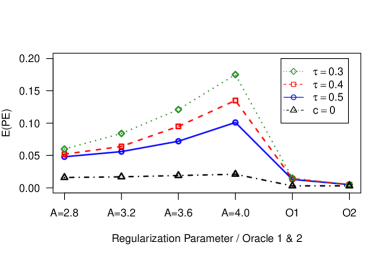
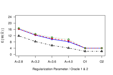
Figure 1. Mean Prediction Errors and Mean $\mathcal{M}(\widehat{\alpha})$

$M=100$

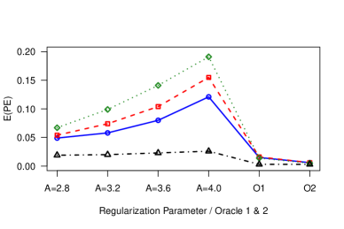
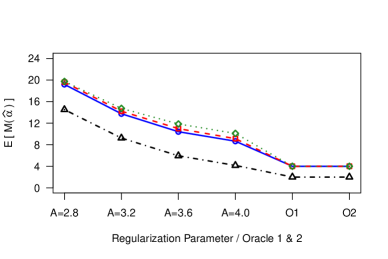
$M=200$

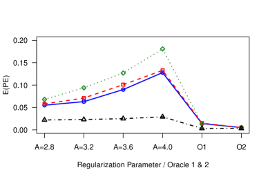
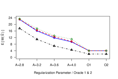
$M=400$

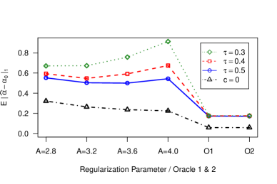
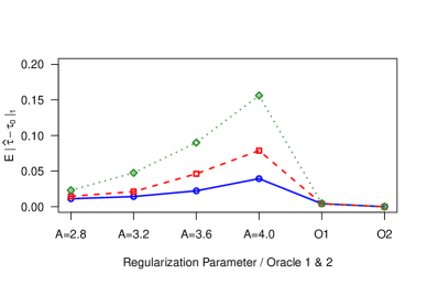
Figure 2. Mean $\ell_{1}$-Errors for $\alpha$ and $\tau$

$M=100$

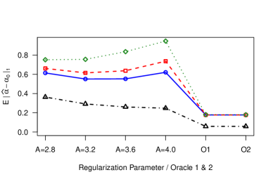
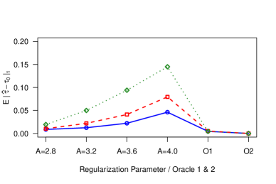
$M=200$

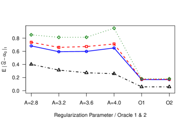
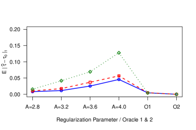
$M=400$

Appendices

We first define some notation used in the appendices. Let $a\vee b\equiv\max\{a,b\}$ and $a\wedge b\equiv\min\{a,b\}$ for any real numbers $a$ and $b$. For two (positive semi-definite) matrices $\mathbf{V}_{1}$ and $\mathbf{V}_{2}$, define the supremum distance $d_{\infty}(\mathbf{V}_{1},\mathbf{V}_{2}):=\max_{j,k}|(\mathbf{V}_{1})_{j,k}-(\mathbf{V}_{2})_{j,k}|$. Let $\widehat{\mathbf{D}}=\mathbf{D}(\widehat{\tau})$ and $\mathbf{D=D}\left(\tau_{0}\right),$ and similarly, let $\widehat{S}_{n}=S_{n}(\widehat{\alpha},\widehat{\tau})$ and $S_{n}=S_{n}\left(\alpha_{0},\tau_{0}\right)$. Recall that $\mathbf{X}(\tau)$ denotes the $(n\times 2M)$ matrix whose $i$-th row is $\mathbf{X}_{i}(\tau)^{\prime}=(X_{i}^{\prime},X_{i}^{\prime}1\{Q_{i}<\tau\})^{\prime}$. Define $X_{\max}:=\max_{\tau,j}\big{\{}\left\|\mathbf{X}^{(j)}(\tau)\right\|_{n},\ \ j=1,...,2M,\tau\in\mathbb{T}\big{\}}$ and $X_{\min}:=\min_{j}\big{\{}\left\|\mathbf{X}^{(j)}(t_{0})\right\|_{n},\ \ j=1,...,2M\big{\}}$ where $t_{0}$ is from $\mathbb{T}\equiv[t_{0},t_{1}]$. Also,  let $\alpha_{\max}$ denote the maximum value that all the elements of $\alpha$ can take in absolute value.

Appendix A Sufficient Conditions for the Uniform Restricted Eigenvalue Assumption

In this section of the appendix, we provide two sets of sufficient conditions for Assumption 2.

A.1. The First Sufficient Condition

The first approach is based on modifications of Assumption 2 of Bickel et al. (2009). We first write $\mathbf{X}\left(\tau\right)=(\mathbf{\tilde{X}},\mathbf{\tilde{X}}\left(\tau\right))$ where $\mathbf{\tilde{X}}$ is the $\left(n\times M\right)$ matrix whose $i$-th row is $X_{i}^{\prime}$, and $\mathbf{\tilde{X}}\left(\tau\right)$ is the $\left(n\times M\right)$ matrix whose $i$-th row is $X_{i}^{\prime}1\{Q_{i}<\tau\}$, respectively. Define the following Gram matrices:

$$\Psi_{n}(\tau) :=n^{-1}\mathbf{X}\left(\tau\right)^{\prime}\mathbf{X}\left(\tau\right),$$

$$\Psi_{n,+}(\tau) :=n^{-1}\mathbf{\tilde{X}}\left(\tau\right)^{\prime}\mathbf{\tilde{X}}\left(\tau\right),$$

$$\Psi_{n,-}(\tau) :=n^{-1}\left[\mathbf{\tilde{X}}-\mathbf{\tilde{X}}\left(\tau\right)\right]^{\prime}\left[\mathbf{\tilde{X}}-\mathbf{\tilde{X}}\left(\tau\right)\right],$$

and define the following restricted eigenvalues:

$$\phi_{\min}\left(u,\tau\right) :=\min_{x\in\mathbb{R}^{2M}:1\leq\mathcal{M}\left(x\right)\leq u}\frac{x^{\prime}\Psi_{n}(\tau)x}{x^{\prime}x},\ \phi_{\max}\left(u,\tau\right):=\max_{x\in\mathbb{R}^{2M}:1\leq\mathcal{M}\left(x\right)\leq u}\frac{x^{\prime}\Psi_{n}(\tau)x}{x^{\prime}x},$$

$$\phi_{\min,+}\left(u,\tau\right) :=\min_{x\in\mathbb{R}^{M}:1\leq\mathcal{M}\left(x\right)\leq u}\frac{x^{\prime}\Psi_{n,+}(\tau)x}{x^{\prime}x},\phi_{\max,+}\left(u,\tau\right):=\max_{x\in\mathbb{R}^{M}:1\leq\mathcal{M}\left(x\right)\leq u}\frac{x^{\prime}\Psi_{n,+}(\tau)x}{x^{\prime}x}$$

and $\phi_{\min,-}\left(u,\tau\right)$ and $\phi_{\max,-}\left(u,\tau\right)$ are defined analogously with $\Psi_{n,-}(\tau)$. Let

$$\kappa_{2}\left(s,m,c_{0},\tau\right) :=\sqrt{\phi_{\min}\left(s+m,\tau\right)}\left(1-c_{0}\sqrt{\frac{s\phi_{\max}\left(m,\tau\right)}{m\phi_{\min}\left(s+m,\tau\right)}}\right),$$

$$\psi :=\min_{\tau\in\mathbb{S}}\frac{\phi_{\max,-}\left(2m,\tau\right)\wedge\phi_{\max,+}\left(2m,\tau\right)}{\phi_{\max,-}\left(2m,\tau\right)\vee\phi_{\max,+}\left(2m,\tau\right)}.$$

Lemma 4.

Assume that the following holds uniformly in $\tau\in\mathbb{S}$:

(A.1) $$\begin{split}m\phi_{\min,+}\left(2s+2m,\tau\right)&>c_{1}^{2}s\phi_{\max,+}\left(2m,\tau\right),\\ m\phi_{\min,-}\left(2s+2m,\tau\right)&>c_{1}^{2}s\phi_{\max,-}\left(2m,\tau\right)\end{split}$$

for some integers $s,m$ such that $1\leq s\leq M/4$, $m\geq s$ and $2s+2m\leq M$ and a constant $c_{1}>0$. Also, assume that $\psi>0.$ Then, Assumption 2 is satisfied with $c_{0}=c_{1}\sqrt{\psi/(1+\psi)}$ and $\kappa\left(s,c_{0},\mathbb{S}\right)=\min_{\tau\in\mathbb{S}}\kappa_{2}\left(s,m,c_{0},\tau\right).$

Conditions in (A.1) are modifications of Assumption 2 of Bickel et al. (2009). Note that for each $\tau\in\mathbb{S}$, data are split into two subsamples with corresponding Gram matrices $\Psi_{n,+}(\tau)$ $\Psi_{n,-}(\tau)$, respectively. Hence, conditions in (A.1) are equivalent to stating that Assumption 2 of Bickel et al. (2009) holds with a universal constant $c_{0}$ for each subsample of all possible sample splitting induced by different values of $\tau\in\mathbb{S}$. As discussed by Bickel et al. (2009), if we take $s+m=s\log n$ and assume that $\phi_{\max,+}(\cdot,\cdot)$ and $\phi_{\max,-}(\cdot,\cdot)$ are uniformly bounded by a constant, conditions in Lemma 4 are equivalent to

$$\min_{\tau\in\mathbb{S}}\log n\left[\phi_{\min,+}(2s\log n,\tau)\wedge\phi_{\min,-}(2s\log n,\tau)\right]>c_{URE},$$

where $c_{URE}>0$ is a constant.

Proof of Lemma 4.

Define $\bar{\mathbf{X}}\left(\tau\right):=(\mathbf{\tilde{X}}-\mathbf{\tilde{X}}\left(\tau\right),\mathbf{\tilde{X}}\left(\tau\right)).$ For any $y=\left(y_{1}^{\prime},y_{2}^{\prime}\right)^{\prime}$ such that $y_{1},y_{2}\in\mathbb{R}^{M}\setminus\{0\}$, let $x_{1}=y_{1}/\sqrt{y^{\prime}y},x_{2}=y_{2}/\sqrt{y^{\prime}y}.$ Then $x_{1}^{\prime}x_{1}+x_{2}^{\prime}x_{2}=1$. Furthermore, since $[\mathbf{\tilde{X}}-\mathbf{\tilde{X}}\left(\tau\right)]^{\prime}\mathbf{\tilde{X}}\left(\tau\right)=0$, we have

$$\frac{y^{\prime}n^{-1}\bar{\mathbf{X}}\left(\tau\right)^{\prime}\bar{\mathbf{X}}\left(\tau\right)y}{y^{\prime}y}=\frac{x_{1}^{\prime}\Psi_{n,-}(\tau)x_{1}}{x_{1}^{\prime}x_{1}}x_{1}^{\prime}x_{1}+\frac{x_{2}^{\prime}\Psi_{n,+}(\tau)x_{2}}{x_{2}^{\prime}x_{2}}x_{2}^{\prime}x_{2}.$$

Also, note that $\mathcal{M}\left(x_{1}\right)$ and $\mathcal{M}\left(x_{2}\right)$ are smaller than or equal to $\mathcal{M}\left(y\right).$

Since any selection of $s$ column vectors in $\mathbf{X}\left(\tau\right)$ can be represented by a linear transformation of a selection of $2s$ column vectors of $\bar{\mathbf{X}}\left(\tau\right)$, the minimum restricted eigenvalue of dimension $2s$ for $\bar{\mathbf{X}}\left(\tau\right)$ can be smaller than that of dimension $s$ for $\mathbf{X}\left(\tau\right)$. Likewise, the maximum restricted eigenvalue of dimension $2s$ for $\bar{\mathbf{X}}\left(\tau\right)$ can be larger than that of dimension $s$ for $\mathbf{X}\left(\tau\right)$. Thus, with $u=2s+2m$,

$$m\min_{y\in\mathbb{R}^{2M}:1\leq\mathcal{M}\left(y\right)\leq s+m}\frac{y^{\prime}n^{-1}\mathbf{X}\left(\tau\right)^{\prime}\mathbf{X}\left(\tau\right)y}{y^{\prime}y} \geq m\min_{y\in\mathbb{R}^{2M}:1\leq\mathcal{M}\left(y\right)\leq u}\frac{y^{\prime}n^{-1}\bar{\mathbf{X}}\left(\tau\right)^{\prime}\bar{\mathbf{X}}\left(\tau\right)y}{y^{\prime}y}$$

$$\geq m\left(\phi_{\min,-}\left(u,\tau\right)\wedge\phi_{\min,+}\left(u,\tau\right)\right)$$

$$> c_{1}^{2}s\left(\phi_{\max,-}\left(2m,\tau\right)\wedge\phi_{\max,+}\left(2m,\tau\right)\right)$$

$$> c_{1}^{2}s\frac{\psi}{1+\psi}\max_{y\in\mathbb{R}^{2M}:1\leq\mathcal{M}\left(y\right)\leq 2m}\frac{y^{\prime}n^{-1}\bar{\mathbf{X}}\left(\tau\right)^{\prime}\bar{\mathbf{X}}\left(\tau\right)y}{y^{\prime}y}$$

$$\geq c_{1}^{2}s\frac{\psi}{1+\psi}\max_{y\in\mathbb{R}^{2M}:1\leq\mathcal{M}\left(y\right)\leq m}\frac{y^{\prime}n^{-1}\mathbf{X}\left(\tau\right)^{\prime}\mathbf{X}\left(\tau\right)y}{y^{\prime}y}.$$

This implies that Bickel et al. (2009)’s Assumption 2 hold for $\mathbf{X}\left(\tau\right)$ with $c_{0}=c_{1}\sqrt{\psi/\left(1+\psi\right)}.$ Then, it follows from their Lemma 4.1 that Assumption 2 is satisfied with $\kappa\left(s,c_{0}\right)=\min_{\tau\in\mathbb{S}}\kappa_{2}\left(s,m,c_{0},\tau\right).$ ∎

A.2. The Second Sufficient Condition

The second approach is in the spirit of Section 10.1 of van de Geer and Bühlmann (2009). In this subsection, we provide primitive sufficient conditions for our simulation designs in Section 6 and Appendix F. In our simulation designs, $X_{i}$ is independent and identically distributed (i.i.d.) as $N(0,\Sigma)$. The independent design case is with $\Sigma=I_{M}$ and the dependent case is with $(\Sigma)_{i,j}=\rho^{|i-j|}$, where $(\Sigma)_{i,j}$ denotes the (i,j) element of the $M\times M$ covariance matrix $\Sigma$. Also, $Q_{i}$ is independent of $X_{i}$ and i.i.d. from $\text{Unif}(0,1)$.

Define $\hat{\mathbf{V}}(\tau):=\mathbf{X}(\tau)^{\prime}\mathbf{X}(\tau)/n$ and $\mathbf{V}(\tau):=\mathbb{E}[\mathbf{X}_{i}(\tau)\mathbf{X}_{i}(\tau)^{\prime}]$. In our simulation designs, $\mathbf{V}(\tau)=\Omega\otimes\Sigma$, where

$$\Omega \equiv\left(\begin{array}[]{cc}1&\tau\\ \tau&\tau\\ \end{array}\right),$$

since $Q_{i}$ and $X_{i}$ are independent of each other and $\mathbb{P}[Q_{i}<\tau]=\tau$.

For a positive semi-definite, $2M\times 2M$ matrix $\mathbf{V}$, define

$$\kappa(\mathbf{V};s,c_{0},\mathbb{S}):=\min_{\tau\in\mathbb{S}}\min_{\begin{subarray}{c}J_{0}\subseteq\{1,\ldots,2M\},\\ |J_{0}|\leq s\end{subarray}}\min_{\begin{subarray}{c}\gamma\neq 0,\\ \left|\gamma_{J_{0}^{c}}\right|_{1}\leq c_{0}\left|\gamma_{J_{0}}\right|_{1}\end{subarray}}\frac{(\gamma^{\prime}\mathbf{V}\gamma)^{1/2}}{|\gamma_{J_{0}}|_{2}}.$$

As in van de Geer and Bühlmann (2009), define the supremum distance:

$$d_{\infty}(\mathbf{V}_{1},\mathbf{V}_{2}):=\max_{j,k}|(\mathbf{V}_{1})_{j,k}-(\mathbf{V}_{2})_{j,k}|$$

for two (positive semi-definite) matrices $\mathbf{V}_{1}$ and $\mathbf{V}_{2}$.

Note that for any $2M$-dimensional, nonzero vector $\gamma$ such that $|\gamma_{J_{0}^{c}}|_{1}\leq c_{0}|\gamma_{J_{0}}|_{1}$, we have that

$$|\gamma^{\prime}(\hat{\mathbf{V}}(\tau)-\mathbf{V}(\tau))\gamma| \leq\sup_{\tau\in\mathbb{T}}d_{\infty}(\hat{\mathbf{V}}(\tau),\mathbf{V}(\tau))|\gamma|_{1}^{2}$$

$$\leq\sup_{\tau\in\mathbb{T}}d_{\infty}(\hat{\mathbf{V}}(\tau),\mathbf{V}(\tau))(1+c_{0})^{2}|\gamma_{J_{0}}|_{1}^{2}$$

$$\leq\sup_{\tau\in\mathbb{T}}d_{\infty}(\hat{\mathbf{V}}(\tau),\mathbf{V}(\tau))(1+c_{0})^{2}s|\gamma_{J_{0}}|_{2}^{2},$$

which implies that

$$\kappa(\hat{\mathbf{V}}(\tau);s,c_{0},\mathbb{S})\geq\kappa(\mathbf{V}(\tau);s,c_{0},\mathbb{S})-(1+c_{0})\sqrt{s\times\sup_{\tau\in\mathbb{T}}d_{\infty}(\hat{\mathbf{V}}(\tau),\mathbf{V}(\tau))}.$$

Hence, our simulation design satisfies Assumption 2 with probability approaching one as $n\rightarrow\infty$ if we establish the following two steps:

1. $\kappa(\mathbf{V}(\tau);s,c_{0},\mathbb{S})>0$ (a population version of the URE condition),

2. $s\times\sup_{\tau\in\mathbb{T}}d_{\infty}(\hat{\mathbf{V}}(\tau),\mathbf{V}(\tau))\rightarrow_{p}0$ as $n\rightarrow\infty$ (uniform convergence in probability of the sample covariance matrix with a rate faster than $s^{-1}$).

Proof of Step 1.

All the eigenvalues of the Kronecker product of $\Omega$ and $\Sigma$ can be written as the product between eigenvalues of $\Omega$ and those of $\Sigma$. First, note that as long as $\tau$ belongs to a strict compact interval between 0 and 1, as in our simulations ($\mathbb{T}\in[0.15,0.85]$), we have strictly positive eigenvalues for $\Omega$. Second, if $\Sigma$ is an identity matrix, then all eigenvalues are 1’s; if $\Sigma$ is a Toeplitz matrix such that $(\Sigma)_{i,j}=\rho^{|i-j|}$, then the smallest eigenvalue of $\Sigma$ is $1-\rho$, independent of the dimension $M$. Hence, in both cases, the smallest eigenvalue of $\mathbf{V}(\tau)$ is bounded away from zero uniformly in $\tau$. Thus, it is clear that $\kappa(\mathbf{V}(\tau);s,c_{0},\mathbb{S})>0$ holds. ∎

To prove the second step, it is sufficient to assume that as $n\rightarrow\infty$, we have that $M\rightarrow\infty$ and that

(A.2) $$s=o\left(\sqrt{\frac{n}{\log nM}}\;\right).$$

Proof of Step 2.

For any $j,k=1,\ldots,M$, define

$$\tilde{V}_{j,k} :=\frac{1}{n}\sum_{i=1}^{n}X_{i}^{(j)}X_{i}^{(k)}-\mathbb{E}[X_{i}^{(j)}X_{i}^{(k)}],$$

$$\hat{V}_{j,k}(\tau) :=\frac{1}{n}\sum_{i=1}^{n}X_{i}^{(j)}X_{i}^{(k)}1\{Q_{i}<\tau\}-\mathbb{E}[X_{i}^{(j)}X_{i}^{(k)}1\{Q_{i}<\tau\}].$$

Note that $s\times\sup_{\tau\in\mathbb{T}}d_{\infty}(\hat{\mathbf{V}}(\tau),\mathbf{V}(\tau))$ is bounded by the maximum between $s\times\max_{j,k}|\tilde{V}_{j,k}|$ and $s\times\max_{j,k}\sup_{\tau\in\mathbb{T}}|\hat{V}_{j,k}(\tau)|$. The former is already shown to be $o_{p}(1)$ by van de Geer and Bühlmann (2009, Section 10.1) under the restriction $s=o\left[(n/\log M)^{1/2}\right]$. Thus, it suffices to show that

(A.3) $$s\times\max_{j,k}\sup_{\tau\in\mathbb{T}}|\hat{V}_{j,k}(\tau)|=o_{p}(1).$$

Since $X_{i}$ is i.i.d. as $N(0,\Sigma)$, $Q_{i}$ i.i.d. as $\text{Unif}(0,1)$, and $Q_{i}$ is independent of $X_{i}$ in our simulation designs, there exists a universal constant $C<\infty$ such that

$$\max_{j,k}\sup_{\tau\in\mathbb{T}}\mathbb{E}\left\{X_{i}^{(j)}X_{i}^{(k)}1\{Q_{i}<\tau\}-\mathbb{E}[X_{i}^{(j)}X_{i}^{(k)}1\{Q_{i}<\tau\}]\right\}^{2}<C.$$

Suppose that $\hat{V}_{j,k}^{\prime}(\tau)$ denotes an independent copy of $\hat{V}_{j,k}(\tau)$. Note that for each $(j,k)$ pair and every $\tau\in\mathbb{T}$, by Chebyshev’s inequality, we have

$$\mathbb{P}\left[|\hat{V}_{j,k}^{\prime}(\tau)|\geq\frac{\varepsilon}{2}\right]\leq\frac{4C}{n\varepsilon^{2}}$$

for every $\varepsilon>0$. Let $\epsilon_{1},\ldots,,\epsilon_{n}$ be a Rademacher sequence independent of the original data. For each $(j,k)$ pair,

$$\mathbb{P}\left[\sup_{\tau\in\mathbb{T}}|\hat{V}_{j,k}(\tau)|\geq\varepsilon\right] \leq\left[1-\frac{4C}{n\varepsilon^{2}}\right]^{-1}P\left[\sup_{\tau\in\mathbb{T}}|\hat{V}_{j,k}(\tau)-\hat{V}_{j,k}^{\prime}(\tau)|\geq\frac{\varepsilon}{2}\right]$$

$$\leq 2\left[1-\frac{4C}{n\varepsilon^{2}}\right]^{-1}\mathbb{P}\left[\sup_{\tau\in\mathbb{T}}\left|\frac{1}{n}\sum_{i=1}^{n}\epsilon_{i}X_{i}^{(j)}X_{i}^{(k)}1\{Q_{i}<\tau\}\right|\geq\frac{\varepsilon}{4}\right],$$

where the first inequality follows from Pollard’s first symmetrization lemma (Pollard, 1984, Lemma II.3.8, page 14), and the second inequality comes from Pollard’s second symmetrization (Pollard, 1984, page 15).

Note that for all $j,k=1,\ldots,M$, $\mathbb{E}\epsilon_{i}X_{i}^{(j)}X_{i}^{(k)}1\{Q_{i}<\tau\}=0$ and that there exists some universal constant $K<\infty$ such that

$$\mathbb{E}\left[\left|\epsilon_{i}X_{i}^{(j)}X_{i}^{(k)}1\{Q_{i}<\tau\}\right|^{m}\right]\leq\frac{m!}{2}K^{m-2}$$

for all $m\geq 2$, for all $\tau\in\mathbb{T}$, and for all $j,k=1,\ldots,M$. Then by Bernstein’s inequality (see e.g. Lemma 14.9. of Bühlmann and van de Geer, 2011), we have, for each $(j,k)$ pair and each $\tau\in\mathbb{T}$,

$$\mathbb{P}\left[\frac{1}{n}\sum_{i=1}^{n}\epsilon_{i}X_{i}^{(j)}X_{i}^{(k)}1\{Q_{i}<\tau\}\geq Kt+\sqrt{2t}\right]\leq\exp(-nt)$$

for any $t>0$. Since $K$ is a universal constant over $(j,k)$ pairs and over $\tau\in\mathbb{T}$ as well, an application of Boole’s inequality yields that

$$\mathbb{P}\left[\max_{j,k}\sup_{\tau\in\mathbb{T}}\frac{1}{n}\sum_{i=1}^{n}\epsilon_{i}X_{i}^{(j)}X_{i}^{(k)}1\{Q_{i}<\tau\}\geq Kt+\sqrt{2t}\right]\leq nM^{2}\exp(-nt)$$

for any $t>0$. Combining all the results above yields

$$\mathbb{P}\left[\max_{j,k}\sup_{\tau\in\mathbb{T}}|\hat{V}_{j,k}(\tau)|\geq 4(Kt+\sqrt{2t})\right] \leq 4\left[1-\frac{4C}{n(Kt+\sqrt{2t})^{2}}\right]^{-1}nM^{2}\exp(-nt)$$

for any $t>0$. Then, under the restriction (A.2), we obtain the desired result by taking $t=\tilde{C}\times{\log nM}/{n}$ for a sufficiently large $\tilde{C}>0$. ∎

Appendix B Discussions on Assumption 3

We provide further discussions on Assumption 3. Assumption 3 is stronger than just the identifiability of $\tau_{0}$ as it specifies the rate of deviation in $f$ as $\tau$ moves away from $\tau_{0}.$ The linear rate here is sharper than the quadratic one that is usually observed in regular M-estimation problems, and it reflects the fact that the limit criterion function, in the classical setup with a fixed number of stochastic regressors, has a kink at the true $\tau_{0}.$

For instance, suppose that $\{(Y_{i},X_{i},Q_{i}):i=1,\ldots,n\}$ are independent and identically distributed, and consider the case where only the intercept is included in $X_{i}$. Assuming that $Q_{i}$ has a density function that is continuous and positive everywhere (so that $\mathbb{P}\left(\tau\leq Q_{i}<\tau_{0}\right)$ and $\mathbb{P}\left(\tau_{0}\leq Q_{i}<\tau\right)$ can be bounded below by $c_{1}\left|\tau-\tau_{0}\right|$ for some $c_{1}>0$), we have that

$$\mathbb{E}\left(Y_{i}-f_{i}\left(\alpha,\tau\right)\right)^{2}-\mathbb{E}\left(Y_{i}-f_{i}\left(\alpha_{0},\tau_{0}\right)\right)^{2}$$

$$= \mathbb{E}\left(f_{i}\left(\alpha_{0},\tau_{0}\right)-f_{i}\left(\alpha,\tau\right)\right)^{2}$$

$$= \left(\alpha_{1}-\alpha_{10}\right)^{2}\mathbb{P}\left(Q_{i}<\tau\wedge\tau_{0}\right)+\left(\alpha_{2}-\alpha_{20}\right)^{2}\mathbb{P}\left(Q_{i}\geq\tau\vee\tau_{0}\right)$$

$$+\left(\alpha_{2}-\alpha_{10}\right)^{2}\mathbb{P}\left(\tau\leq Q_{i}<\tau_{0}\right)+\left(\alpha_{1}-\alpha_{20}\right)^{2}\mathbb{P}\left(\tau_{0}\leq Q_{i}<\tau\right)$$

$$\geq c\left|\tau-\tau_{0}\right|,$$

for some $c>0,$ where $f_{i}\left(\alpha,\tau\right)=X_{i}^{\prime}\beta+X_{i}^{\prime}\delta 1\{Q_{i}<\tau\}$, $\alpha_{1}=\beta+\delta\$and $\alpha_{2}=\beta,$ unless $\left|\alpha_{2}-\alpha_{10}\right|$ is too small when $\tau<\tau_{0}$ and $\left|\alpha_{1}-\alpha_{20}\right|$ is too small when $\tau>\tau_{0}.$ However, when $\left|\alpha_{2}-\alpha_{10}\right|$ is small, say smaller than $\varepsilon,$ $\left|\alpha_{2}-\alpha_{20}\right|$ is bounded above zero due to the discontinuity that $\alpha_{10}\neq\alpha_{20}$ and $\mathbb{P}\left(Q_{i}\geq\tau\vee\tau_{0}\right)=\mathbb{P}\left(Q_{i}\geq\tau_{0}\right)$ is also bounded above zero. This implies the inequality still holds. Since the same reasoning applies for the latter case, we can conclude our discontinuity assumption holds in the standard discontinuous threshold regression setup. In other words, the previous literature has typically imposed conditions sufficient enough to render this condition.

B.1. Verification of Assumption 3 for the Simulation Design of Section 6

In this subsection, we may provide more primitive discussions for our simulation design in Section 6, where $X_{i}\sim N\left(0,I_{M}\right)$ and $Q_{i}\sim\text{Unif}(0,1)$ independent of $X_{i}$ and $U_{i}\sim N\left(0,\sigma^{2}\right)$ independent of $\left(X_{i},Q_{i}\right).$ For simplicity, suppose that $\beta_{0}=0$ and $\delta_{0}=\left(c_{0},0,...,0\right)^{\prime}$ for $c_{0}\neq 0$ and $\tau_{0}=0.5.$ Recall that $\mathbb{T}=[0.15,0.85]$ in our simulation design. As our theoretical framework is deterministic design, we may check if Assumption 3 is satisfied with probability approaching one as $n\rightarrow\infty.$

We only consider the case of $\tau<\tau_{0}$ explicitly below. The other case is similar. Note that when $\tau<\tau_{0}$,

$$\left\|f_{\alpha,\tau}-f_{0}\right\|_{n}^{2} =\frac{1}{n}\sum_{i=1}^{n}\left(X_{i}^{\prime}1\left\{Q_{i}<\tau\right\}\left(\beta+\delta-\beta_{0}-\delta_{0}\right)\right)^{2}$$

$$+\frac{1}{n}\sum_{i=1}^{n}\left(X_{i}^{\prime}1\left\{Q_{i}\geq\tau_{0}\right\}\left(\beta-\beta_{0}\right)\right)^{2}$$

$$+\frac{1}{n}\sum_{i=1}^{n}\left(X_{i}^{\prime}1\left\{\tau\leq Q_{i}<\tau_{0}\right\}\left(\beta-\beta_{0}-\delta_{0}\right)\right)^{2}.$$

Then, under our specification of the data generating process,

$$\mathbb{E}\left\|f_{\alpha,\tau}-f_{0}\right\|_{n}^{2}$$

$$=\tau\left(\beta+\delta-\beta_{0}-\delta_{0}\right)^{\prime}\left(\beta+\delta-\beta_{0}-\delta_{0}\right)+(1-\tau_{0})\left(\beta-\beta_{0}\right)^{\prime}\left(\beta-\beta_{0}\right)$$

$$+(\tau_{0}-\tau)\left(\beta-\beta_{0}-\delta_{0}\right)^{\prime}\left(\beta-\beta_{0}-\delta_{0}\right)$$

$$\geq(1-\tau_{0})\left(\beta-\beta_{0}\right)^{\prime}\left(\beta-\beta_{0}\right)+(\tau_{0}-\tau)\left(\beta-\beta_{0}-\delta_{0}\right)^{\prime}\left(\beta-\beta_{0}-\delta_{0}\right)$$

$$=(1-\tau_{0})\beta^{\prime}\beta+(\tau_{0}-\tau)\left(\beta-\delta_{0}\right)^{\prime}\left(\beta-\delta_{0}\right)$$

$$=c_{0}^{2}\left(\tau_{0}-\tau\right)+\beta^{\prime}\beta\left(1-\tau\right)-2\beta^{\prime}\delta_{0}\left(\tau_{0}-\tau\right).$$

If $\beta^{\prime}\beta\left(1-\tau\right)-2\beta^{\prime}\delta_{0}\left(\tau_{0}-\tau\right)\geq 0$, Assumption 3 is satisfied with probability approaching one as $n\rightarrow\infty$.

Suppose not. Then, we must have that $\beta^{\prime}\beta\left(1-\tau\right)<2\beta^{\prime}\delta_{0}\left(\tau_{0}-\tau\right)=2\beta_{1}c_{0}\left(\tau_{0}-\tau\right)$ for some nonzero $\beta_{1}$, which is the first element of $\beta$. Hence,

$$\beta^{\prime}\beta<2|\beta_{1}||c_{0}|\frac{\tau_{0}-\tau}{1-\tau}$$

Now note that

$$\left|\beta_{1}\right|\leq\frac{\beta^{\prime}\beta}{\left|\beta_{1}\right|}\leq 2|c_{0}|\frac{\tau_{0}-\tau}{1-\tau}\leq|c_{0}|\frac{0.7}{0.85}\;\text{ for any $\tau\in\mathbb{T}=[0.15,0.85]$},$$

which implies that

$$\mathbb{E}\left\|f_{\alpha,\tau}-f_{0}\right\|_{n}^{2} \geq\left(c_{0}-\beta_{1}\right)^{2}\left(\tau_{0}-\tau\right)+\beta^{\prime}\beta(1-\tau)-\beta_{1}^{2}\left(\tau_{0}-\tau\right)$$

$$\geq\left(\frac{0.15}{0.85}\right)^{2}c_{0}^{2}\left(\tau-\tau_{0}\right),$$

where the last inequality follows from the simple fact that $\beta^{\prime}\beta(1-\tau)\geq\beta_{1}^{2}\left(\tau_{0}-\tau\right)$.

Appendix C Proofs for Section 4

In this section of the appendix, we prove the prediction consistency of our Lasso estimator. Let

$$V_{1j} :=\left(n\sigma\left\|X^{(j)}\right\|_{n}\right)^{-1}\sum_{i=1}^{n}U_{i}X_{i}^{(j)},$$

$$V_{2j}(\tau) :=\left(n\sigma\left\|X^{(j)}(\tau)\right\|_{n}\right)^{-1}\sum_{i=1}^{n}U_{i}X_{i}^{(j)}1\{Q_{i}<\tau\}.$$

For a constant $\mu\in(0,1)$, define the events

$$\mathbb{A} :=\bigcap_{j=1}^{M}\left\{2|V_{1j}|\leq\mu\lambda/\sigma\right\},$$

$$\mathbb{B} :=\bigcap_{j=1}^{M}\left\{2\sup_{\tau\in\mathbb{T}}|V_{2j}(\tau)|\leq\mu\lambda/\sigma\right\},$$

Also define $J_{0}:=J(\alpha_{0})$ and $R_{n}:=R_{n}(\alpha_{0},\tau_{0}),$ where

$$R_{n}(\alpha,\tau):=2n^{-1}\sum_{i=1}^{n}U_{i}X_{i}^{\prime}\delta\left\{1(Q_{i}<\widehat{\tau})-1(Q_{i}<\tau)\right\}.$$

The following lemma gives some useful inequalities that provide a basis for all our theoretical results.

Lemma 5 (Basic Inequalities).

Conditional on the events $\mathbb{A}$ and $\mathbb{B}$, we have

(C.1) $$\left\|\widehat{f}-f_{0}\right\|_{n}^{2}+\left(1-\mu\right)\lambda\left|\widehat{\mathbf{D}}(\widehat{\alpha}-\alpha_{0})\right|_{1} \leq 2\lambda\left|\widehat{\mathbf{D}}(\widehat{\alpha}-\alpha_{0})_{J_{0}}\right|_{1}$$

$$+\lambda\left|\left|\widehat{\mathbf{D}}{\alpha_{0}}\right|_{1}-\left|\mathbf{D}{\alpha_{0}}\right|_{1}\right|+R_{n}$$

and

(C.2) $$\left\|\widehat{f}-f_{0}\right\|_{n}^{2}+\left(1-\mu\right)\lambda\left|\widehat{\mathbf{D}}(\widehat{\alpha}-\alpha_{0})\right|_{1}\leq 2\lambda\left|\widehat{\mathbf{D}}(\widehat{\alpha}-\alpha_{0})_{J_{0}}\right|_{1}+\left\|f_{(\alpha_{0},\widehat{\tau})}-f_{0}\right\|_{n}^{2}.$$

The basic inequalities in Lemma 5 involve more terms than that of the linear model (e.g. Lemma 6.1 of Bühlmann and van de Geer, 2011) because our model in (1.1) includes the unknown threshold parameter $\tau_{0}$ and the weighted Lasso is considered in (2.2). Also, it helps prove our main results to have different upper bounds in (C.1) and (C.2) for the same lower bound.

Proof of Lemma 5.

Note that

(C.3) $$\widehat{S}_{n}+\lambda\left|\widehat{\mathbf{D}}\widehat{\alpha}\right|_{1}\leq S_{n}(\alpha,\tau)+\lambda\left|\mathbf{D}(\tau)\alpha\right|_{1}$$

for all $(\alpha,\tau)\in\mathbb{R}^{2M}\times\mathbb{T}.$ Now write

$$\widehat{S}_{n}-S_{n}(\alpha,\tau)$$

$$=n^{-1}\left|\mathbf{y}-\mathbf{X}(\widehat{\tau})\widehat{\alpha}\right|_{2}^{2}-n^{-1}\left|\mathbf{y}-\mathbf{X}(\tau)\alpha\right|_{2}^{2}$$

$$=n^{-1}\sum_{i=1}^{n}\left[U_{i}-\left\{\mathbf{X}_{i}(\widehat{\tau})^{\prime}\widehat{\alpha}-\mathbf{X}_{i}(\tau_{0})^{\prime}\alpha_{0}\right\}\right]^{2}-n^{-1}\sum_{i=1}^{n}\left[U_{i}-\left\{\mathbf{X}_{i}(\tau)^{\prime}\alpha-\mathbf{X}_{i}(\tau_{0})^{\prime}\alpha_{0}\right\}\right]^{2}$$

$$=n^{-1}\sum_{i=1}^{n}\left\{\mathbf{X}_{i}(\widehat{\tau})^{\prime}\widehat{\alpha}-\mathbf{X}_{i}(\tau_{0})^{\prime}\alpha_{0}\right\}^{2}-n^{-1}\sum_{i=1}^{n}\left\{\mathbf{X}_{i}(\tau)^{\prime}\alpha-\mathbf{X}_{i}(\tau_{0})^{\prime}\alpha_{0}\right\}^{2}$$

$$\;\;\;-2n^{-1}\sum_{i=1}^{n}U_{i}\left\{\mathbf{X}_{i}(\widehat{\tau})^{\prime}\widehat{\alpha}-\mathbf{X}_{i}(\tau)^{\prime}\alpha\right\}$$

$$=\left\|\widehat{f}-f_{0}\right\|_{n}^{2}-\left\|f_{(\alpha,\tau)}-f_{0}\right\|_{n}^{2}$$

$$\;\;\;-2n^{-1}\sum_{i=1}^{n}U_{i}X_{i}^{\prime}(\widehat{\beta}-\beta)-2n^{-1}\sum_{i=1}^{n}U_{i}\left\{X_{i}^{\prime}\widehat{\delta}1(Q_{i}<\widehat{\tau})-X_{i}^{\prime}\delta 1(Q_{i}<\tau)\right\}.$$

Further, write the last term above as

$$n^{-1}\sum_{i=1}^{n}U_{i}\left\{X_{i}^{\prime}\widehat{\delta}1(Q_{i}<\widehat{\tau})-X_{i}^{\prime}\delta 1(Q_{i}<\tau)\right\}$$

$$=n^{-1}\sum_{i=1}^{n}U_{i}X_{i}^{\prime}(\widehat{\delta}-\delta)1(Q_{i}<\widehat{\tau})+n^{-1}\sum_{i=1}^{n}U_{i}X_{i}^{\prime}\delta\left\{1(Q_{i}<\widehat{\tau})-1(Q_{i}<\tau)\right\}.$$

Hence, (C.3) can be written as

$$\begin{split}\left\|\widehat{f}-f_{0}\right\|_{n}^{2}&\leq\left\|f_{(\alpha,\tau)}-f_{0}\right\|_{n}^{2}+\lambda\left|\mathbf{D}(\tau)\alpha\right|_{1}-\lambda\left|\widehat{\mathbf{D}}\widehat{\alpha}\right|_{1}\\ &+2n^{-1}\sum_{i=1}^{n}U_{i}X_{i}^{\prime}(\widehat{\beta}-\beta)+2n^{-1}\sum_{i=1}^{n}U_{i}X_{i}^{\prime}(\widehat{\delta}-\delta)1(Q_{i}<\widehat{\tau})\\ &+2n^{-1}\sum_{i=1}^{n}U_{i}X_{i}^{\prime}\delta\left\{1(Q_{i}<\widehat{\tau})-1(Q_{i}<\tau)\right\}.\end{split}$$

Then on the events $\mathbb{A}$ and $\mathbb{B}$, we have

(C.4) $$\begin{split}\left\|\widehat{f}-f_{0}\right\|_{n}^{2}&\leq\left\|f_{(\alpha,\tau)}-f_{0}\right\|_{n}^{2}+\mu\lambda\left|\widehat{\mathbf{D}}(\widehat{\alpha}-\alpha)\right|_{1}\\ &+\lambda\left|\mathbf{D}(\tau)\alpha\right|_{1}-\lambda\left|\widehat{\mathbf{D}}\widehat{\alpha}\right|_{1}+R_{n}(\alpha,\tau)\end{split}$$

for all $(\alpha,\tau)\in\mathbb{R}^{2M}\times\mathbb{T}.$

Note the fact that

(C.5) $$\left|\widehat{\alpha}^{(j)}-\alpha_{0}^{(j)}\right|+\left|\alpha_{0}^{(j)}\right|-\left|\widehat{\alpha}^{(j)}\right|=0\text{ for $j\notin J_{0}$}.$$

On the one hand, by (C.4) (evaluating at $(\alpha,\tau)=(\alpha_{0},\tau_{0})$), on the events $\mathbb{A}$ and $\mathbb{B}$,

$$\begin{split}\@ADDCLASS{ltx_eqn_lefteqn}$\displaystyle\left\|\widehat{f}-f_{0}\right\|_{n}^{2}+\left(1-\mu\right)\lambda\left|\mathbf{\hat{D}}(\widehat{\alpha}-\alpha_{0})\right|_{1}$\mbox{}\hfil\\ &\leq\lambda\left(\left|\widehat{\mathbf{D}}(\widehat{\alpha}-\alpha_{0})\right|_{1}+\left|\widehat{\mathbf{D}}\alpha_{0}\right|_{1}-\left|\widehat{\mathbf{D}}\widehat{\alpha}\right|_{1}\right)\\ &+\lambda\left|\left|\widehat{\mathbf{D}}{\alpha_{0}}\right|_{1}-\left|\mathbf{D}{\alpha_{0}}\right|_{1}\right|+R_{n}(\alpha_{0},\tau_{0})\\ &\leq 2\lambda\left|\widehat{\mathbf{D}}(\widehat{\alpha}-\alpha_{0})_{J_{0}}\right|_{1}+\lambda\left|\left|\widehat{\mathbf{D}}{\alpha_{0}}\right|_{1}-\left|\mathbf{D}{\alpha_{0}}\right|_{1}\right|+R_{n}(\alpha_{0},\tau_{0}),\end{split}$$

which proves $\left(\ref{imp-ineq-lem}\right)$. On the other hand, again by (C.4) (evaluating at $(\alpha,\tau)=(\alpha_{0},\widehat{\tau})$), on the events $\mathbb{A}$ and $\mathbb{B}$,

$$\begin{split}\@ADDCLASS{ltx_eqn_lefteqn}$\displaystyle\left\|\widehat{f}-f_{0}\right\|_{n}^{2}+\left(1-\mu\right)\lambda\left|\mathbf{\hat{D}}(\widehat{\alpha}-\alpha_{0})\right|_{1}$\mbox{}\hfil\\ &\leq\lambda\left(\left|\widehat{\mathbf{D}}(\widehat{\alpha}-\alpha_{0})\right|_{1}+\left|\widehat{\mathbf{D}}\alpha_{0}\right|_{1}-\left|\widehat{\mathbf{D}}\widehat{\alpha}\right|_{1}\right)+\left\|f_{(\alpha_{0},\widehat{\tau})}-f_{0}\right\|_{n}^{2}\\ &\leq 2\lambda\left|\widehat{\mathbf{D}}(\widehat{\alpha}-\alpha_{0})_{J_{0}}\right|_{1}+\left\|f_{(\alpha_{0},\widehat{\tau})}-f_{0}\right\|_{n}^{2},\end{split}$$

which proves $\left(\ref{imp-ineq-2-lem}\right)$. ∎

We now establish conditions under which $\mathbb{A}\cap\mathbb{B}$ has probability close to one with a suitable choice of $\lambda$. Let $\Phi$ denote the cumulative distribution function of the standard normal.

Lemma 6 (Probability of $\mathbb{A}\cap\mathbb{B}$).

Let $\{U_{i}:i=1,\ldots,n\}$ be independent and identically distributed as $\mathbf{N}(0,\sigma^{2})$. Then

$$\mathbb{P}\{\mathbb{A}\cap\mathbb{B}\}\geq 1-6M\Phi\left(-\frac{\mu\sqrt{nr_{n}}}{2\sigma}\lambda\right).$$

Recall that $r_{n}$ depends on the lower bound $t_{0}$ of the parameter space for $\tau_{0}$. Suppose that $t_{0}$ is taken such that $t_{0}<\min_{i=1,\ldots,n}Q_{i}$. Then $\left\|X^{\left(j\right)}(t_{0})\right\|_{n}=0$, and therefore, $r_{n}=0$. In this case, Lemma 6 reduces to $\mathbb{P}\{\mathbb{A}\cap\mathbb{B}\}\geq 1-3M$ regardless of $n$ and $\lambda$, hence resulting in a useless bound. This illustrates a need for restricting the parameter space for $\tau_{0}$ (see Assumption 1).

Proof of Lemma 6.

Since $U_{i}\sim\mathbf{N}(0,\sigma^{2})$,

$$\mathbb{P}\{\mathbb{A}^{c}\}\leq\sum_{j=1}^{M}\mathbb{P}\left\{\sqrt{n}|V_{1j}|>\mu\sqrt{n}\lambda/(2\sigma)\right\}=2M\Phi\left(-\frac{\mu\sqrt{n}}{2\sigma}\lambda\right)\leq 2M\Phi\left(-\frac{\mu\sqrt{r_{n}n}}{2\sigma}\lambda\right),$$

where the last inequality follows from $0<r_{n}\leq 1$.

Now consider the event $\mathbb{B}$. For the simplify of notation, we assume without loss of generality that $Q_{i}=i/n$ since there is no tie among $Q_{i}$’s. Note that $\left\|X^{\left(j\right)}(\tau)\right\|_{n}$ is monotonically increasing in $\tau$ and $\sum_{i=1}^{n}U_{i}X_{i}^{\left(j\right)}1\left\{Q_{i}<\tau\right\}$ can be rewritten as a partial sum process by the rearrangement of $i$ according to the magnitude of $Q_{i}.$ To see the latter, given $\left\{Q_{i}\right\}$, let $\ell$ be the index $i$ such that $Q_{i}$ is the $\ell$-th smallest of $\left\{Q_{i}\right\}.$ Since $\left\{U_{i}\right\}$ is an independent and identically distributed (i.i.d.) sequence and $Q_{i}$ is deterministic, $\left\{U_{\ell}\right\}_{\ell=1,...,n}$ is also an i.i.d. sequence. Furthermore, $U_{\ell}X_{\ell}^{\left(j\right)}$ is a sequence of independent and symmetric random variables as $U_{\ell}$ is Gaussian and $X$ is a deterministic design. Thus, it satisfies the conditions for Lévy’s inequality (see e.g. Proposition A.1.2 of van der Vaart and Wellner, 1996). Then, by Lévy’s inequality,

$$\mathbb{P}\left\{\sup_{\tau\in\mathbb{T}}\sqrt{n}\left|V_{2j}(\tau)\right|>\mu\sqrt{n}\lambda/(2\sigma)\right\} \leq\mathbb{P}\left\{\sup_{1\leq s\leq n}\left|\frac{1}{\sigma\sqrt{n}}\sum_{i=1}^{s}U_{i}X_{i}^{\left(j\right)}\right|>\left\|X^{\left(j\right)}\left(t_{0}\right)\right\|_{n}\frac{\mu\sqrt{n}}{2\sigma}\lambda\right\}$$

$$\leq 2\mathbb{P}\left\{\sqrt{n}|V_{1j}|>\frac{\left\|X^{\left(j\right)}(t_{0})\right\|_{n}}{\left\|X^{\left(j\right)}\right\|_{n}}\frac{\mu\sqrt{n}}{2\sigma}\lambda\right\}.$$

Therefore, we have

$$\mathbb{P}\{\mathbb{B}^{c}\} \leq\sum_{j=1}^{M}\mathbb{P}\left\{\sup_{\tau\in\mathbb{T}}\sqrt{n}|V_{2j}(\tau)|>\mu\sqrt{n}\lambda/(2\sigma)\right\}$$

$$\leq 4M\Phi\left(-\frac{\mu\sqrt{r_{n}n}}{2\sigma}\lambda\right).$$

Since $\mathbb{P}\{\mathbb{A}\cap\mathbb{B}\}\geq 1-\mathbb{P}\{\mathbb{A}^{c}\}-\mathbb{P}\{\mathbb{B}^{c}\}$, we have proved the lemma. ∎

We are ready to establish the prediction consistency of the Lasso estimator. Recall that $X_{\max}:=\max_{\tau,j}\big{\{}\left\|\mathbf{X}^{(j)}(\tau)\right\|_{n},\ \ j=1,...,2M,\tau\in\mathbb{T}\big{\}}$ and $X_{\min}:=\min_{j}\big{\{}\left\|\mathbf{X}^{(j)}(t_{0})\right\|_{n},\\ \ \ j=1,...,2M\big{\}}$, that $\alpha_{\max}$ denotes the maximum value that all the elements of $\alpha$ can take in absolute value, and that Assumption 1 implies that $r_{n}>0$ and also $X_{\min}>0$.

Lemma 7 (Consistency of the Lasso).

Let $(\widehat{\alpha},\widehat{\tau})$ be the Lasso estimator defined by (2.5) with $\lambda$ given by (4.2). Then, with probability at least $1-\left(3M\right)^{1-A^{2}\mu^{2}/8}$, we have

$$\left\|\widehat{f}-f_{0}\right\|_{n} \leq\Big{(}6\lambda X_{\max}\alpha_{\max}\mathcal{M}(\alpha_{0})+2\mu\lambda X_{\max}\left|\delta_{0}\right|_{1}\Big{)}^{1/2}.$$

Proof of Lemma 7.

Note that

$$R_{n}=2n^{-1}\sum_{i=1}^{n}U_{i}X_{i}^{\prime}\delta_{0}\left\{1(Q_{i}<\widehat{\tau})-1(Q_{i}<\tau_{0})\right\}.$$

Then on the event $\mathbb{B}$,

(C.6) $$\begin{split}|R_{n}|&\leq 2\mu\lambda\sum_{j=1}^{M}\left\|X^{(j)}\right\|_{n}|\delta_{0}^{(j)}|\\ &\leq 2\mu\lambda X_{\max}\left|\delta_{0}\right|_{1}.\end{split}$$

Then, conditional on $\mathbb{A}\cap\mathbb{B}$, combining (C.6) with (C.1) gives

(C.7) $$\left\|\widehat{f}-f_{0}\right\|_{n}^{2}+\left(1-\mu\right)\lambda\left|\widehat{\mathbf{D}}(\widehat{\alpha}-\alpha_{0})\right|_{1}\leq 6\lambda X_{\max}\alpha_{\max}\mathcal{M}(\alpha_{0})+2\mu\lambda X_{\max}\left|\delta_{0}\right|_{1}$$

since

$$\left|\widehat{\mathbf{D}}(\widehat{\alpha}-\alpha_{0})_{J_{0}}\right|_{1} \leq 2X_{\max}\alpha_{\max}\mathcal{M}(\alpha_{0}),$$

$$\left|\left|\widehat{\mathbf{D}}{\alpha_{0}}\right|_{1}-\left|\mathbf{D}{\alpha_{0}}\right|_{1}\right| \leq 2X_{\max}\left|\alpha_{0}\right|_{1}.$$

Using the bound that $2\Phi\left(-x\right)\leq\exp\left(-x^{2}/2\right)$ for $x\geq(2/\pi)^{1/2}$ as in equation (B.4) of Bickel et al. (2009), Lemma 6 with $\lambda$ given by (4.2) implies that the event $\mathbb{A}\cap\mathbb{B}$ occurs with probability at least $1-\left(3M\right)^{1-A^{2}\mu^{2}/8}$. Then the lemma follows from (C.7). ∎

Proof of Theorem 1.

The proof follows immediately from combining Assumption 1 with Lemma 7. In particular, for the value of $K_{1}$, note that since $\left|\delta_{0}\right|_{1}\leq\alpha_{\max}\mathcal{M}(\alpha_{0})$,

$$6\lambda X_{\max}\alpha_{\max}\mathcal{M}(\alpha_{0})+2\mu\lambda X_{\max}\left|\delta_{0}\right|_{1} \leq\lambda\mathcal{M}\left(\alpha_{0}\right)\left(6X_{\max}\alpha_{\max}+2\mu X_{\max}\alpha_{\max}\right)$$

$$\leq\lambda\mathcal{M}\left(\alpha_{0}\right)\left(6C_{2}C_{1}+2\mu C_{2}C_{1}\right),$$

where the last inequality follows from Assumption 1. Therefore, we set

$$K_{1} :=\sqrt{2C_{1}C_{2}(3+\mu)}.$$

∎

Appendix D Proofs for Section 5.1

We first provide a lemma to derive an oracle inequality regarding the sparsity of the Lasso estimator $\widehat{\alpha}$.

Lemma 8 (Sparsity of the Lasso).

Conditional on the event $\mathbb{A}\bigcap\mathbb{B}$, we have

(D.1) $$\mathcal{M}(\widehat{\alpha})\leq\frac{4\phi_{\max}}{\left(1-\mu\right)^{2}\lambda^{2}X_{\min}^{2}}\left\|\widehat{f}-f_{0}\right\|_{n}^{2}.$$

Proof of Lemma 8.

As in (B.6) of Bickel et al. (2009), for each $\tau$, the necessary and sufficient condition for $\widehat{\alpha}(\tau)$ to be the Lasso solution can be written in the form

$$\frac{2}{n}[X^{(j)}]^{\prime}(\mathbf{y}-\mathbf{X}(\tau)\widehat{\alpha}(\tau)) =\lambda\left\|X^{(j)}\right\|_{n}\text{sign}(\widehat{\beta}^{(j)}(\tau)) \widehat{\beta}^{(j)}(\tau) \neq 0$$ if

$$\left|\frac{2}{n}[X^{(j)}]^{\prime}(\mathbf{y}-\mathbf{X}(\tau)\widehat{\alpha}(\tau))\right| \leq\lambda\left\|X^{(j)}\right\|_{n} \widehat{\beta}^{(j)}(\tau) =0$$ if

$$\frac{2}{n}[X^{(j)}(\tau)]^{\prime}(\mathbf{y}-\mathbf{X}(\tau)\widehat{\alpha}(\tau)) =\lambda\left\|X^{(j)}(\tau)\right\|_{n}\text{sign}(\widehat{\delta}^{(j)}(\tau)) \widehat{\delta}^{(j)}(\tau) \neq 0$$ if

$$\left|\frac{2}{n}[X^{(j)}(\tau)]^{\prime}(\mathbf{y}-\mathbf{X}(\tau)\widehat{\alpha}(\tau))\right| \leq\lambda\left\|X^{(j)}(\tau)\right\|_{n} \widehat{\delta}^{(j)}(\tau) \text{$=0$},$$ if

where $j=1,\ldots,M$.

Note that conditional on events $\mathbb{A}$ and $\mathbb{B}$,

$$\left|\frac{2}{n}\sum_{i=1}^{n}U_{i}X_{i}^{(j)}\right| \leq\mu\lambda\left\|X^{(j)}\right\|_{n}$$

$$\left|\frac{2}{n}\sum_{i=1}^{n}U_{i}X_{i}^{(j)}1\{Q_{i}<\tau\}\right| \leq\mu\lambda\left\|X^{(j)}(\tau)\right\|_{n}$$

for any $\tau$, where $j=1,\ldots,M$. Therefore,

$$\left|\frac{2}{n}[X^{(j)}]^{\prime}(\mathbf{X}(\tau_{0})\alpha_{0}-\mathbf{X}(\tau)\widehat{\alpha}(\tau))\right| \geq\left(1-\mu\right)\lambda\left\|X^{(j)}\right\|_{n} \widehat{\beta}^{(j)}(\tau) \neq 0$$ if

$$\left|\frac{2}{n}[X^{(j)}(\tau)]^{\prime}(\mathbf{X}(\tau_{0})\alpha_{0}-\mathbf{X}(\tau)\widehat{\alpha}(\tau))\right| \geq\left(1-\mu\right)\lambda\left\|X^{(j)}(\tau)\right\|_{n} \widehat{\delta}^{(j)}(\tau) \text{$\neq 0$}.$$ if

Using inequalities above, write

$$\frac{1}{n^{2}}\left[\mathbf{X}(\tau_{0})\alpha_{0}-\mathbf{X}(\widehat{\tau})\widehat{\alpha}\right]^{\prime}\mathbf{X}(\widehat{\tau})\mathbf{X}(\widehat{\tau})^{\prime}\left[\mathbf{X}(\tau_{0})\alpha_{0}-\mathbf{X}(\widehat{\tau})\widehat{\alpha}\right]$$

$$=\frac{1}{n^{2}}\sum_{j=1}^{M}\left\{[X^{(j)}]^{\prime}[\mathbf{X}(\tau_{0})\alpha_{0}-\mathbf{X}(\widehat{\tau})\widehat{\alpha}]\right\}^{2}+\frac{1}{n^{2}}\sum_{j=1}^{M}\left\{[X^{(j)}(\widehat{\tau})]^{\prime}[\mathbf{X}(\tau_{0})\alpha_{0}-\mathbf{X}(\widehat{\tau})\widehat{\alpha}]\right\}^{2}$$

$$\geq\frac{1}{n^{2}}\sum_{j:\widehat{\beta}^{(j)}\neq 0}\left\{[X^{(j)}]^{\prime}[\mathbf{X}(\tau_{0})\alpha_{0}-\mathbf{X}(\widehat{\tau})\widehat{\alpha}]\right\}^{2}+\frac{1}{n^{2}}\sum_{j:\widehat{\delta}^{(j)}\neq 0}\left\{[X^{(j)}(\widehat{\tau})]^{\prime}[\mathbf{X}(\tau_{0})\alpha_{0}-\mathbf{X}(\widehat{\tau})\widehat{\alpha}]\right\}^{2}$$

$$\geq\frac{\left(1-\mu\right)^{2}\lambda^{2}}{4}\left(\sum_{j:\widehat{\beta}^{(j)}\neq 0}\left\|X^{(j)}\right\|_{n}^{2}+\sum_{j:\widehat{\delta}^{(j)}\neq 0}\left\|X^{(j)}(\widehat{\tau})\right\|_{n}^{2}\right)$$

$$\geq\frac{\left(1-\mu\right)^{2}\lambda^{2}}{4}X_{\min}^{2}\mathcal{M}\left(\hat{\alpha}\right).$$

To complete the proof, note that

$$\frac{1}{n^{2}} \left[\mathbf{X}(\tau_{0})\alpha_{0}-\mathbf{X}(\widehat{\tau})\widehat{\alpha}\right]^{\prime}\mathbf{X}(\widehat{\tau})\mathbf{X}(\widehat{\tau})^{\prime}\left[\mathbf{X}(\tau_{0})\alpha_{0}-\mathbf{X}(\widehat{\tau})\widehat{\alpha}\right]$$

$$\leq\text{maxeig}(\mathbf{X}(\widehat{\tau})\mathbf{X}(\widehat{\tau})^{\prime}/n)\left\|\widehat{f}-f_{0}\right\|_{n}^{2}$$

$$\leq\phi_{\max}\left\|\widehat{f}-f_{0}\right\|_{n}^{2},$$

where $\text{maxeig}(\mathbf{X}(\widehat{\tau})\mathbf{X}(\widehat{\tau})^{\prime}/n)$ denotes the largest eigenvalue of $\mathbf{X}(\widehat{\tau})\mathbf{X}(\widehat{\tau})^{\prime}/n$. ∎

Lemma 9.

Suppose that $\delta_{0}=0$. Let Assumption 2 hold with $\kappa=\kappa(s,\frac{1+\mu}{1-\mu},\mathbb{T})$ for $\mu<1$, and $\mathcal{M}(\alpha_{0})\leq s\leq M$. Let $(\widehat{\alpha},\widehat{\tau})$ be the Lasso estimator defined by (2.5) with $\lambda$ given by (4.2). Then, with probability at least $1-\left(3M\right)^{1-A^{2}\mu^{2}/8},$ we have

$$\left\|\widehat{f}-f_{0}\right\|_{n} \leq\frac{2A\sigma X_{\max}}{\kappa}\left(\frac{\log 3M}{nr_{n}}s\right)^{1/2},$$

$$\left|\widehat{\alpha}-\alpha_{0}\right|_{1} \leq\frac{4A\sigma}{\left(1-\mu\right)\kappa^{2}}\frac{X_{\max}^{2}}{X_{\min}}\left(\frac{\log 3M}{nr_{n}}\right)^{1/2}s,$$

$$\mathcal{M}(\widehat{\alpha}) \leq\frac{16\phi_{\max}}{\left(1-\mu\right)^{2}\kappa^{2}}\frac{X_{\max}^{2}}{X_{\min}^{2}}s.$$

Proof of Lemma 9.

Note that $\delta_{0}=0$ implies $\left\|f_{(\alpha_{0},\widehat{\tau})}-f_{0}\right\|^{2}=0$. Combining this with (C.2), we have

(D.2) $$\left\|\widehat{f}-f_{0}\right\|_{n}^{2}+\left(1-\mu\right)\lambda\left|\widehat{\mathbf{D}}(\widehat{\alpha}-\alpha_{0})\right|_{1}\leq 2\lambda\left|\widehat{\mathbf{D}}(\widehat{\alpha}-\alpha_{0})_{J_{0}}\right|_{1},$$

which implies that

$$\left|\widehat{\mathbf{D}}(\widehat{\alpha}-\alpha_{0})_{J_{0}^{c}}\right|_{1}\leq\frac{1+\mu}{1-\mu}\left|\widehat{\mathbf{D}}(\widehat{\alpha}-\alpha_{0})_{J_{0}}\right|_{1}.$$

This in turn allows us to apply Assumption 2, specifically URE$(s,\frac{1+\mu}{1-\mu},\mathbb{T})$, to yield

(D.3) $$\begin{split}\kappa^{2}\left|\widehat{\mathbf{D}}(\widehat{\alpha}-\alpha_{0})_{J_{0}}\right|_{2}^{2}&\leq\frac{1}{n}|\mathbf{X}(\widehat{\tau})\widehat{\mathbf{D}}(\widehat{\alpha}-\alpha_{0})|_{2}^{2}\\ &=\frac{1}{n}(\widehat{\alpha}-\alpha_{0})^{\prime}\widehat{\mathbf{D}}\mathbf{X}(\widehat{\tau})^{\prime}\mathbf{X}(\widehat{\tau})\widehat{\mathbf{D}}(\widehat{\alpha}-\alpha_{0})\\ &\leq\frac{\max(\widehat{\mathbf{D}})^{2}}{n}(\widehat{\alpha}-\alpha_{0})^{\prime}\mathbf{X}(\widehat{\tau})^{\prime}\mathbf{X}(\widehat{\tau})(\widehat{\alpha}-\alpha_{0})\\ &=\max(\widehat{\mathbf{D}})^{2}\left\|\widehat{f}-f_{0}\right\|_{n}^{2},\end{split}$$

where $\kappa=\kappa(s,\frac{1+\mu}{1-\mu},\mathbb{T})$ and the last equality is due to the assumption that $\delta_{0}=0$.

Combining (D.2) with (D.3) yields

$$\left\|\widehat{f}-f_{0}\right\|_{n}^{2} \leq 2\lambda\left|\widehat{\mathbf{D}}(\widehat{\alpha}-\alpha_{0})_{J_{0}}\right|_{1}$$

$$\leq 2\lambda\sqrt{s}\left|\widehat{\mathbf{D}}(\widehat{\alpha}-\alpha_{0})_{J_{0}}\right|_{2}$$

$$\leq\frac{2\lambda}{\kappa}\sqrt{s}\max(\widehat{\mathbf{D}})\left\|\widehat{f}-f_{0}\right\|_{n}.$$

Then the first conclusion of the lemma follows immediately.

In addition, combining the arguments above with the first conclusion of the lemma yields

(D.4) $$\begin{split}\left|\widehat{\mathbf{D}}\left(\widehat{\alpha}-\alpha_{0}\right)\right|_{1}&=\left|\widehat{\mathbf{D}}(\widehat{\alpha}-\alpha_{0})_{J_{0}}\right|_{1}+\left|\widehat{\mathbf{D}}(\widehat{\alpha}-\alpha_{0})_{J_{0}^{c}}\right|_{1}\\ &\leq 2\left(1-\mu\right)^{-1}\left|\widehat{\mathbf{D}}(\widehat{\alpha}-\alpha_{0})_{J_{0}}\right|_{1}\\ &\leq 2\left(1-\mu\right)^{-1}\sqrt{s}\left|\widehat{\mathbf{D}}(\widehat{\alpha}-\alpha_{0})_{J_{0}}\right|_{2}\\ &\leq\frac{2}{\kappa\left(1-\mu\right)}\sqrt{s}\max(\widehat{\mathbf{D}})\left\|\widehat{f}-f_{0}\right\|_{n}\\ &\leq\frac{4\lambda}{\left(1-\mu\right)\kappa^{2}}{s}X_{\max}^{2},\end{split}$$

which proves the second conclusion of the lemma since

(D.5) $$\left|\widehat{\mathbf{D}}\left(\widehat{\alpha}-\alpha_{0}\right)\right|_{1}\geq\min(\widehat{\mathbf{D}})\left|\widehat{\alpha}-\alpha_{0}\right|_{1}.$$

Finally, the lemma follows by Lemma 8 with the bound on $\mathbb{P}(\mathbb{A}\cap\mathbb{B})$ as in the proof of Lemma 7. ∎

Proof of Theorem 2.

The proof follows immediately from combining Assumption 1 with Lemma 9. In particular, the constant $K_{2}$ can be chosen as

$$K_{2} \equiv\max\left(2AC_{2},\frac{4AC_{2}^{2}}{(1-\mu)C_{3}},\frac{16C_{2}^{2}}{(1-\mu)^{2}C_{3}^{2}}\right).$$

∎

Appendix E Proofs for Section 5.2

To simplify notation, in this section, we assume without loss of generality that $Q_{i}=i/n$. Then $\mathbb{T}=[t_{0},t_{1}]\subset(0,1)$. For some constant $\eta>0$, define an event

$$\mathbb{C}\left(\eta\right):=\left\{\sup_{\left|\tau-\tau_{0}\right|<\eta}\left|\frac{2}{n}\sum_{i=1}^{n}U_{i}X_{i}^{\prime}\delta_{0}\left[1\left(Q_{i}<\tau_{0}\right)-1\left(Q_{i}<\tau\right)\right]\right|\leq\lambda\sqrt{\eta}\right\}.$$

Recall that $h_{n}\left(\eta\right):=\left(\left(2n\eta\right)^{-1}\sum_{i=\max\{1,\left[n\left(\tau_{0}-\eta\right)\right]\}}^{\min\{\left[n\left(\tau_{0}+\eta\right)\right],n\}}\left(X_{i}^{\prime}\delta_{0}\right)^{2}\right)^{1/2}$.

The following lemma gives the lower bound of the probability of the event $\mathbb{A}\cap\mathbb{B}\cap[\cap_{j=1}^{m}\mathbb{C}(\eta_{j})]$ for a given $m$ and some positive constants $\eta_{1},...,\eta_{m}$. To deal with the event $\cap_{j=1}^{m}\mathbb{C}(\eta_{j})$, an extra term is added to the lower bound of the probability, in comparison to Lemma 6.

Lemma 10 (Probability of $\mathbb{A}\cap\mathbb{B}\cap\{\cap_{j=1}^{m}\mathbb{C}(\eta_{j})\}$).

For a given $m$ and some positive constants $\eta_{1},...,\eta_{m}$ such that $h_{n}\left(\eta_{j}\right)>0$ for each $j=1,\ldots,m$,

$$\mathbb{P}\left\{\mathbb{A\bigcap B}\bigcap\left[\bigcap_{j=1}^{m}\mathbb{C}\left(\eta_{j}\right)\right]\right\}\geq 1-6M\Phi\left(-\frac{\mu\sqrt{nr_{n}}}{2\sigma}\lambda\right)-4\sum_{j=1}^{m}\Phi\left(-\frac{\lambda\sqrt{n}}{2\sqrt{2}\sigma h_{n}\left(\eta_{j}\right)}\right).$$

Proof of Lemma 10.

Given Lemma 6, it remains to examine the probability of $\mathbb{C}\left(\eta_{j}\right)$. As in the proof of Lemma 6, Lévy’s inequality yields that

$$\mathbb{P}\left\{\mathbb{C}\left(\eta_{j}\right)^{c}\right\} \leq \mathbb{P}\left\{\sup_{\left|\tau-\tau_{0}\right|\leq\eta_{j}}\left|\frac{2}{n}\sum_{i=1}^{n}U_{i}X_{i}^{\prime}\delta_{0}\left[1\left(Q_{i}<\tau_{0}\right)-1\left(Q_{i}<\tau\right)\right]\right|>\lambda\sqrt{\eta_{j}}\right\}.$$

$$\leq 2\mathbb{P}\left\{\left|\frac{2}{n}\sum_{i=\left[n\left(\tau_{0}-\eta_{j}\right)\right]}^{\left[n\left(\tau_{0}+\eta_{j}\right)\right]}U_{i}X_{i}^{\prime}\delta_{0}\right|>\lambda\sqrt{\eta_{j}}\right\}$$

$$\leq 4\Phi\left(-\frac{\lambda\sqrt{n}}{2\sqrt{2}\sigma h_{n}\left(\eta_{j}\right)}\right).$$

Hence, we have proved the lemma since $\mathbb{P}\left\{\mathbb{A\bigcap B}\bigcap\left[\bigcap_{j=1}^{m}\mathbb{C}\left(\eta_{j}\right)\right]\right\}\geq 1-\mathbb{P}\{\mathbb{A}^{c}\}-\mathbb{P}\{\mathbb{B}^{c}\}-\sum_{j=1}^{m}\mathbb{P}\{\mathbb{C}\left(\eta_{j}\right)^{c}\}$. ∎

The following lemma gives an upper bound of $\left|\widehat{\tau}-\tau_{0}\right|$ using only Assumption 3, conditional on the events $\mathbb{A}$ and $\mathbb{B}$.

Lemma 11.

Suppose that Assumption 3 holds. Let

$$\eta^{\ast}=\max\left\{\min_{i}\left|Q_{i}-\tau_{0}\right|,c^{-1}\lambda\left(6X_{\max}\alpha_{\max}\mathcal{M}(\alpha_{0})+2\mu X_{\max}\left|\delta_{0}\right|_{1}\right)\right\},$$

where $c$ is the constant defined in Assumption 3. Then conditional on the events $\mathbb{A}$ and $\mathbb{B}$,

$$\left|\widehat{\tau}-\tau_{0}\right|\leq\eta^{\ast}.$$

Proof of Lemma 11.

As in the proof of Lemma 5, we have, on the events $\mathbb{A}$ and $\mathbb{B}$,

(E.1) $$\begin{split}\@ADDCLASS{ltx_eqn_lefteqn}$\displaystyle\widehat{S}_{n}-S_{n}(\alpha_{0},\tau_{0})$\mbox{}\hfil\\ &=\left\|\widehat{f}-f_{0}\right\|_{n}^{2}-2n^{-1}\sum_{i=1}^{n}U_{i}X_{i}^{\prime}(\widehat{\beta}-\beta_{0})-2n^{-1}\sum_{i=1}^{n}U_{i}X_{i}^{\prime}(\widehat{\delta}-\delta_{0})1(Q_{i}<\widehat{\tau})-R_{n}\\ &\geq\left\|\widehat{f}-f_{0}\right\|_{n}^{2}-\mu\lambda\left|\widehat{\mathbf{D}}(\widehat{\alpha}-\alpha_{0})\right|_{1}-R_{n}.\end{split}$$

Then using (C.5), on the events $\mathbb{A}$ and $\mathbb{B}$,

(E.2) $$\begin{split}\@ADDCLASS{ltx_eqn_lefteqn}$\displaystyle\left[\widehat{S}_{n}+\lambda\left|\widehat{\mathbf{D}}\widehat{\alpha}\right|_{1}\right]-\left[S_{n}(\alpha_{0},\tau_{0})+\lambda\left|\mathbf{D}\alpha_{0}\right|_{1}\right]$\mbox{}\hfil\\ &\geq\left\|\widehat{f}-f_{0}\right\|_{n}^{2}-\mu\lambda\left|\widehat{\mathbf{D}}(\widehat{\alpha}-\alpha_{0})\right|_{1}-\lambda\left[\left|\mathbf{D}\alpha_{0}\right|_{1}-\left|\widehat{\mathbf{D}}\widehat{\alpha}\right|_{1}\right]-R_{n}\\ &\geq\left\|\widehat{f}-f_{0}\right\|_{n}^{2}-2\lambda\left|\widehat{\mathbf{D}}(\widehat{\alpha}-\alpha_{0})_{J_{0}}\right|_{1}-\lambda\left[\left|\mathbf{D}\alpha_{0}\right|_{1}-\left|\widehat{\mathbf{D}}\alpha_{0}\right|_{1}\right]-R_{n}\\ &\geq\left\|\widehat{f}-f_{0}\right\|_{n}^{2}-\left[6\lambda X_{\max}\alpha_{\max}\mathcal{M}(\alpha_{0})+2\mu\lambda X_{\max}\left|\delta_{0}\right|_{1}\right],\end{split}$$

where the last inequality comes from (C.6) and following bounds:

$$2\lambda\left|\widehat{\mathbf{D}}(\widehat{\alpha}-\alpha_{0})_{J_{0}}\right|_{1} \leq 4\lambda X_{\max}\alpha_{\max}\mathcal{M}\left(\alpha_{0}\right),$$

$$\lambda\left|\left|\mathbf{D}\alpha_{0}\right|_{1}-\left|\widehat{\mathbf{D}}\alpha_{0}\right|_{1}\right| \leq 2\lambda X_{\max}\alpha_{\max}\mathcal{M}\left(\alpha_{0}\right).$$

Suppose now that $\left|\hat{\tau}-\tau_{0}\right|>\eta^{\ast}$. Then Assumption 3 and (E.2) together imply that

$$\left[\widehat{S}_{n}+\lambda\left|\widehat{\mathbf{D}}\widehat{\alpha}\right|_{1}\right]-\left[S_{n}(\alpha_{0},\tau_{0})+\lambda\left|\mathbf{D}\alpha_{0}\right|_{1}\right]>0,$$

which leads to contradiction as $\widehat{\tau}$ is the minimizer of the criterion function as in (2.5). Therefore, we have proved the lemma. ∎

Remark 3.

The nonasymptotic bound in Lemma 11 can be translated into the consistency of $\widehat{\tau}$, as in Lemma 7. That is, if $n\rightarrow\infty$, $M\rightarrow\infty$, and $\lambda\mathcal{M}(\alpha_{0})\rightarrow 0$, Lemma 11 implies the consistency of $\widehat{\tau}$, provided that $X_{\max}$, $\alpha_{\max}$, and $c^{-1}$ are bounded uniformly in $n$ and $Q_{i}$ is continuously distributed.

We now provide a lemma for bounding the prediction risk as well as the $\ell_{1}$ estimation loss for $\alpha_{0}$.

Lemma 12.

Suppose that $\left|\hat{\tau}-\tau_{0}\right|\leq c_{\tau}$ and $\left|\hat{\alpha}-\alpha_{0}\right|_{1}\leq c_{\alpha}$ for some $(c_{\tau},c_{\alpha})$. Suppose further that Assumption 4 and Assumption 2 hold with $\mathbb{S}=\left\{\left|\tau-\tau_{0}\right|\leq c_{\tau}\right\}$, $\kappa=\kappa(s,\frac{2+\mu}{1-\mu},\mathbb{S})$ for $0<\mu<1$ and $\mathcal{M}(\alpha_{0})\leq s\leq M$. Then, conditional on $\mathbb{A}$, $\mathbb{B\ }$and $\mathbb{C}(c_{\tau})$, we have

$$\left\|\widehat{f}-f_{0}\right\|_{n}^{2} \leq 3\lambda\left\{\sqrt{c_{\tau}}+\left(2X_{\min}\right)^{-1}c_{\tau}C\left|\delta_{0}\right|_{1}\vee\frac{6X_{\max}^{2}}{\kappa^{2}}\lambda s\vee\frac{2X_{\max}}{\kappa}\left(c_{\alpha}c_{\tau}C\left|\delta_{0}\right|_{1}s\right)^{1/2}\right\},$$

$$\left|\widehat{\alpha}-\alpha_{0}\right|_{1} \leq\frac{3}{(1-\mu)X_{\min}}\left\{\sqrt{c_{\tau}}+\left(2X_{\min}\right)^{-1}c_{\tau}C\left|\delta_{0}\right|_{1}\vee\frac{6X_{\max}^{2}}{\kappa^{2}}\lambda s\vee\frac{2X_{\max}}{\kappa}\left(c_{\alpha}c_{\tau}C\left|\delta_{0}\right|_{1}s\right)^{1/2}\right\}.$$

Lemma 12 states the bounds for both $\left\|\widehat{f}-f_{0}\right\|_{n}$ and $\left|\widehat{\alpha}-\alpha_{0}\right|_{1}$ may become smaller as $c_{\tau}$ gets smaller. This is because decreasing $c_{\tau}$ reduces the first and third terms in the bounds directly, and also because decreasing $c_{\tau}$ reduces the second term in the bound indirectly by allowing for a possibly larger $\kappa$ since $\mathbb{S}$ gets smaller.

Proof of Lemma 12.

Note that on $\mathbb{C}$,

$$\left|R_{n}\right| = \left|2n^{-1}\sum_{i=1}^{n}U_{i}X_{i}^{\prime}\delta_{0}\left\{1(Q_{i}<\widehat{\tau})-1(Q_{i}<\tau_{0})\right\}\right|$$

$$\leq \lambda\sqrt{c_{\tau}}.$$

The triangular inequality, the mean value theorem (applied to $f\left(x\right)=\sqrt{x}$), and Assumption 4 imply that

(E.3) $$\begin{split}\left|\left|\widehat{\mathbf{D}}{\alpha_{0}}\right|_{1}-\left|\mathbf{D}{\alpha_{0}}\right|_{1}\right|&=\left|\sum_{j=1}^{M}\left(\left\|X^{\left(j\right)}\left(\hat{\tau}\right)\right\|_{n}-\left\|X^{\left(j\right)}\left(\tau_{0}\right)\right\|_{n}\right)\left|\delta_{0}^{\left(j\right)}\right|\right|\\ &\leq\sum_{j=1}^{M}\left(2\left\|X^{\left(j\right)}\left(t_{0}\right)\right\|_{n}\right)^{-1}\left|\delta_{0}^{\left(j\right)}\right|\frac{1}{n}\sum_{i=1}^{n}\left|X_{i}^{\left(j\right)}\right|^{2}\left|1\left\{Q_{i}<\hat{\tau}\right\}-1\left\{Q_{i}<\tau_{0}\right\}\right|\\ &\leq\left(2X_{\min}\right)^{-1}c_{\tau}C\left|\delta_{0}\right|_{1}.\end{split}$$

We now consider two cases: (i) $\left|\widehat{\mathbf{D}}(\widehat{\alpha}-\alpha_{0})_{J_{0}}\right|_{1}>\sqrt{c_{\tau}}+\left(2X_{\min}\right)^{-1}c_{\tau}C\left|\delta_{0}\right|_{1}$ and
(ii) $\left|\widehat{\mathbf{D}}(\widehat{\alpha}-\alpha_{0})_{J_{0}}\right|_{1}\leq\sqrt{c_{\tau}}+\left(2X_{\min}\right)^{-1}c_{\tau}C\left|\delta_{0}\right|_{1}$.

Case (i): In this case, note that

$$\lambda\left|\left|\widehat{\mathbf{D}}\alpha_{0}\right|_{1}-\left|\mathbf{D}\alpha_{0}\right|_{1}\right|+R_{n} <\lambda(2X_{\min})^{-1}c_{\tau}C\left|\delta_{0}\right|_{1}+\lambda\sqrt{c_{\tau}}$$

$$=\lambda\left(\sqrt{c_{\tau}}+(2X_{\min})^{-1}c_{\tau}C\left|\delta_{0}\right|_{1}\right)$$

$$<\lambda\left|\widehat{\mathbf{D}}\left(\widehat{\alpha}-\alpha_{0}\right)_{J_{0}}\right|_{1}.$$

Combining this result with (C.1), we have

(E.4) $$\left\|\widehat{f}-f_{0}\right\|_{n}^{2}+\left(1-\mu\right)\lambda\left|\widehat{\mathbf{D}}(\widehat{\alpha}-\alpha_{0})\right|_{1} \leq 3\lambda\left|\widehat{\mathbf{D}}(\widehat{\alpha}-\alpha_{0})_{J_{0}}\right|_{1},$$

which implies

$$\left|\widehat{\mathbf{D}}(\widehat{\alpha}-\alpha_{0})_{J_{0}^{c}}\right|_{1}\leq\frac{2+\mu}{1-\mu}\left|\widehat{\mathbf{D}}(\widehat{\alpha}-\alpha_{0})_{J_{0}}\right|_{1}.$$

Then, we apply Assumption 2 with URE$(s,\frac{2+\mu}{1-\mu},\mathbb{S})$. Note that since it is assumed that $|\widehat{\tau}-\tau_{0}|\leq c_{\tau}$, Assumption 2 only needs to hold with $\mathbb{S}$ in the $c_{\tau}$ neighborhood of $\tau_{0}$. Since $\delta_{0}\neq 0$, (D.3) now has an extra term

$$\kappa^{2}\left|\widehat{\mathbf{D}}(\widehat{\alpha}-\alpha_{0})_{J_{0}}\right|_{2}^{2}$$

$$\leq\max(\widehat{\mathbf{D}})^{2}\left\|\hat{f}-f_{0}\right\|_{n}^{2}$$

$$\;\;\;+\max(\widehat{\mathbf{D}})^{2}\frac{1}{n}\sum_{i=1}^{n}\bigg{\{}2\Big{(}\mathbf{X}_{i}(\widehat{\tau})^{\prime}\widehat{\alpha}-\mathbf{X}_{i}(\widehat{\tau})^{\prime}\alpha_{0}\Big{)}\Big{(}X_{i}^{\prime}\delta_{0}\big{[}1(Q_{i}<\tau_{0})-1(Q_{i}<\widehat{\tau})\big{]}\Big{)}\bigg{\}}$$

$$\leq\max(\widehat{\mathbf{D}})^{2}\left(\left\|\hat{f}-f_{0}\right\|_{n}^{2}+2c_{\alpha}\left|\delta_{0}\right|_{1}\sup_{j}\frac{1}{n}\sum_{i=1}^{n}\left|{X}_{i}^{(j)}\right|^{2}\left|1(Q_{i}<\tau_{0})-1(Q_{i}<\widehat{\tau})\right|\right)$$

$$\leq X_{\max}^{2}\bigg{(}\left\|\widehat{f}-f_{0}\right\|_{n}^{2}+2c_{\alpha}c_{\tau}C\left|\delta_{0}\right|_{1}\bigg{)},$$

where the last inequality is due to Assumption 4. Combining this result with (E.4), we have

$$\left\|\widehat{f}-f_{0}\right\|_{n}^{2} \leq 3\lambda\left|\widehat{\mathbf{D}}\left(\widehat{\alpha}-\alpha_{0}\right)_{J_{0}}\right|_{1}$$

$$\leq 3\lambda\sqrt{s}\left|\widehat{\mathbf{D}}\left(\widehat{\alpha}-\alpha_{0}\right)_{J_{0}}\right|_{2}$$

$$\leq 3\lambda\sqrt{s}\left(\kappa^{-2}X_{\max}^{2}\left(\left\|\widehat{f}-f_{0}\right\|_{n}^{2}+2c_{\alpha}c_{\tau}C\left|\delta_{0}\right|_{1}\right)\right)^{1/2}.$$

Applying $a+b\leq 2a\vee 2b$, we get the upper bound of $\left\|\widehat{f}-f_{0}\right\|_{n}$ on $\mathbb{A}$ and $\mathbb{B}$, as

(E.5) $$\left\|\widehat{f}-f_{0}\right\|_{n}^{2}\leq\frac{18X_{\max}^{2}}{\kappa^{2}}\lambda^{2}s\vee\frac{6X_{\max}}{\kappa}\lambda\left(c_{\alpha}c_{\tau}C\left|\delta_{0}\right|_{1}s\right)^{1/2}.$$

To derive the upper bound for $\left|\widehat{\alpha}-\alpha_{0}\right|_{1}$, note that using the same arguments as in (D.4),

$$\left|\widehat{D}(\widehat{\alpha}-\alpha_{0})\right|_{1} \leq\frac{3}{1-\mu}\left|\widehat{D}\left(\widehat{\alpha}-\alpha_{0}\right)_{J_{0}}\right|_{1}$$

$$\leq\frac{3}{1-\mu}\sqrt{s}\left|\widehat{D}\left(\widehat{\alpha}-\alpha_{0}\right)_{J_{0}}\right|_{2}$$

$$\leq\frac{3}{1-\mu}\sqrt{s}\left(\kappa^{-2}X_{\max}^{2}\left(\left\|\widehat{f}-f_{0}\right\|_{n}^{2}+2c_{\alpha}c_{\tau}C\left|\delta_{0}\right|_{1}\right)\ \right)^{1/2}$$

$$\leq\frac{3\sqrt{s}}{(1-\mu)\kappa}X_{\max}\left(\left\|\widehat{f}-f_{0}\right\|_{n}^{2}+2c_{\alpha}c_{\tau}C\left|\delta_{0}\right|_{1}\right)^{1/2}.$$

Then combining the fact that $a+b\leq 2a\vee 2b$ with (D.5) and (E.5) yields

$$\left|\widehat{\alpha}-\alpha_{0}\right|_{1} \leq\frac{18}{(1-\mu)\kappa^{2}}\frac{X_{\max}^{2}}{X_{\min}}\lambda s\vee\frac{6}{(1-\mu)\kappa}\frac{X_{\max}}{X_{\min}}\left(c_{\alpha}c_{\tau}C\left|\delta_{0}\right|_{1}s\right)^{1/2}.$$

Case (ii): In this case, it follows directly from (C.1) that

$$\left\|\widehat{f}-f_{0}\right\|_{n}^{2} \leq 3\lambda\left(\sqrt{c_{\tau}}+\left(2X_{\min}\right)^{-1}c_{\tau}C\left|\delta_{0}\right|_{1}\right),$$

$$\left|\widehat{\alpha}-\alpha_{0}\right|_{1} \leq\frac{3}{(1-\mu)X_{\min}}\left(\sqrt{c_{\tau}}+\left(2X_{\min}\right)^{-1}c_{\tau}C\left|\delta_{0}\right|_{1}\right),$$

which establishes the desired result. ∎

The following lemma shows that the bound for $\left|\hat{\tau}-\tau_{0}\right|$ can be further tightened if we combine results obtained in Lemmas 11 and 12.

Lemma 13.

Suppose that $\left|\hat{\tau}-\tau_{0}\right|\leq c_{\tau}$ and $\left|\hat{\alpha}-\alpha_{0}\right|_{1}\leq c_{\alpha}$ for some $(c_{\tau},c_{\alpha})$. Let $\tilde{\eta}:=c^{-1}\lambda\left(\left(1+\mu\right)X_{\max}c_{\alpha}+\sqrt{c_{\tau}}+(2X_{\min})^{-1}c_{\tau}C\left|\delta_{0}\right|_{1}\right)$. If Assumption 3 holds, then conditional on the events $\mathbb{A}$, $\mathbb{B}$, and $\mathbb{C}(c_{\tau})$,

$$\left|\hat{\tau}-\tau_{0}\right|\leq\tilde{\eta}.$$

Proof of Lemma 13.

Note that on $\mathbb{A}$, $\mathbb{B\ }$and $\mathbb{C}$,

$$\left|\frac{2}{n}\sum_{i=1}^{n}\left[U_{i}X_{i}^{\prime}\left(\hat{\beta}-\beta_{0}\right)+U_{i}X_{i}^{\prime}1\left(Q_{i}<\hat{\tau}\right)\left(\hat{\delta}-\delta_{0}\right)\right]\right|$$

$$\leq \mu\lambda X_{\max}\left|\hat{\alpha}-\alpha_{0}\right|_{1}\leq\mu\lambda X_{\max}c_{\alpha}$$

and

$$\left|\frac{2}{n}\sum_{i=1}^{n}U_{i}X_{i}^{\prime}\delta_{0}\left[1\left(Q_{i}<\hat{\tau}\right)-1\left(Q_{i}<\tau_{0}\right)\right]\right|\leq\lambda\sqrt{c_{\tau}}.$$

Suppose $\tilde{\eta}<\left|\hat{\tau}-\tau_{0}\right|<c_{\tau}.$ Then, as in (E.1),

$$\widehat{S}_{n}-S_{n}(\alpha_{0},\tau_{0})\geq\left\|\widehat{f}-f_{0}\right\|_{n}^{2}-\mu\lambda X_{\max}c_{\alpha}-\lambda\sqrt{c_{\tau}}.$$

Furthermore, we obtain

$$\left[\widehat{S}_{n}+\lambda\left|\widehat{\mathbf{D}}\widehat{\alpha}\right|_{1}\right]-\left[S_{n}(\alpha_{0},\tau_{0})+\lambda\left|\mathbf{D}\alpha_{0}\right|_{1}\right]$$

$$\geq\left\|\widehat{f}-f_{0}\right\|_{n}^{2}-\mu\lambda X_{\max}c_{\alpha}-\lambda\sqrt{c_{\tau}}$$

$$-\lambda\left(\left|\widehat{\mathbf{D}}(\widehat{\alpha}-\alpha_{0})\right|_{1}+\left|(\widehat{\mathbf{D}}-\mathbf{D})\alpha_{0}\right|_{1}\right)$$

$$>c\tilde{\eta}-\left(\left(1+\mu\right)X_{\max}c_{\alpha}+\sqrt{c_{\tau}}+(2X_{\min})^{-1}c_{\tau}C\left|\delta_{0}\right|_{1}\right)\lambda,$$

where the last inequality is due to Assumption 3 and (E.3).

Since $c\tilde{\eta}=\left(\left(1+\mu\right)X_{\max}c_{\alpha}+\sqrt{c_{\tau}}+(2X_{\min})^{-1}c_{\tau}C\left|\delta_{0}\right|_{1}\right)\lambda$, we again use the contradiction argument as in the proof of Lemma 11 to establish the result. ∎

Lemma 12 provides us with three different bounds for $\left|\hat{\alpha}-\alpha_{0}\right|_{1}$ and the two of them are functions of $c_{\tau}$ and $c_{\alpha}.$ This leads us to apply Lemmas 12 and 13 iteratively to tighten up the bounds. Furthermore, when the sample size is large and thus $\lambda$ in (4.2) is small enough, we show that the consequence of this chaining argument is that the bound for $\left|\hat{\alpha}-\alpha_{0}\right|$ is dominated by the middle term in Lemma 12. We give exact conditions for this on $\lambda$ and thus on the sample size $n.$ To do so, we first define some constants:

$$A_{1\ast}:=\frac{3\left(1+\mu\right)X_{\max}}{\left(1-\mu\right)X_{\min}}+1,A_{2\ast}:=\frac{C}{2cX_{\min}},A_{3\ast}:=\frac{6cX_{\max}^{2}}{\kappa^{2}},\ \ \text{and}\ \ A_{4\ast}:=\frac{36\left(1+\mu\right)X_{\max}^{3}}{(1-\mu)^{2}X_{\min}}.$$

Assumption 6 (Inequality Conditions).

The following inequalities hold:

(E.6) $$A_{1\ast}A_{2\ast}\lambda\left|\delta_{0}\right|_{1} <1,$$

(E.7) $$\frac{A_{1\ast}}{\left(1-A_{1\ast}A_{2\ast}\lambda\left|\delta_{0}\right|_{1}\right)^{2}} <A_{3\ast}s,$$

(E.8) $$\left(2\kappa^{-2}A_{4\ast}s+1\right)A_{2\ast}\lambda\left|\delta_{0}\right|_{1} <1,$$

(E.9) $$\frac{A_{2\ast}\lambda\left|\delta_{0}\right|_{1}}{\left[1-\left(2\kappa^{-2}A_{4\ast}s+1\right)A_{2\ast}\lambda\left|\delta_{0}\right|_{1}\right]^{2}} <\frac{(1-\mu)c}{4},$$

(E.10) $$\left[1-\left(2\kappa^{-2}A_{4\ast}s+1\right)A_{2\ast}\lambda\left|\delta_{0}\right|_{1}\right]^{-2} <A_{1\ast}A_{3\ast}s.$$

Remark 4.

It would be easier to satisfy Assumption 6 when the sample size $n$ is large. To appreciate Assumption 6 in a setup when $n$ is large, suppose that (1) $n\rightarrow\infty$, $M\rightarrow\infty$, $s\rightarrow\infty$, and $\lambda\rightarrow 0$; (2) $\left|\delta_{0}\right|_{1}$ may or may not diverge to infinity; (3) $X_{\min}$, $X_{\max}$, $\kappa$, $c$, $C$, and $\mu$ are independent of $n$. Then conditions in Assumption 6 can hold simultaneously for all sufficiently large $n$, provided that $s\lambda\left|\delta_{0}\right|_{1}\rightarrow 0$.

We now give the main result of this section.

Lemma 14.

Suppose that Assumption 2 hold with $\mathbb{S}=\left\{\left|\tau-\tau_{0}\right|\leq\eta^{\ast}\right\}$, $\kappa=\kappa(s,\frac{2+\mu}{1-\mu},\mathbb{S})$ for $0<\mu<1,$ and $\mathcal{M}(\alpha_{0})\leq s\leq M$. In addition, Assumptions 3, 4, and 6 hold. Let $(\widehat{\alpha},\widehat{\tau})$ be the Lasso estimator defined by (2.5) with $\lambda$ given by (4.2). Then, there exists a sequence of constants $\eta_{1},...,\eta_{m^{\ast}}$ for some finite $m^{\ast}$ such that $h_{n}\left(\eta_{j}\right)>0$ for each $j=1,\ldots,m^{\ast}$, with probability at least $1-\left(3M\right)^{1-A^{2}\mu^{2}/8}-4\sum_{j=1}^{m^{\ast}}\left(3M\right)^{-A^{2}/(16r_{n}h_{n}\left(\eta_{j}\right))},$ we have

$$\left\|\widehat{f}-f_{0}\right\|_{n} \leq\frac{3A\sigma X_{\max}}{\kappa}\left(\frac{2\log 3M}{nr_{n}}s\right)^{1/2},$$

$$\left|\widehat{\alpha}-\alpha_{0}\right|_{1} \leq\frac{18A\sigma}{\left(1-\mu\right)\kappa^{2}}\frac{X_{\max}^{2}}{X_{\min}}\left({\frac{\log 3M}{nr_{n}}}\right)^{1/2}s,$$

$$\left|\hat{\tau}-\tau_{0}\right| \leq\left(\frac{3\left(1+\mu\right)X_{\max}}{(1-\mu)X_{\min}}+1\right)\frac{6X_{\max}^{2}A^{2}\sigma^{2}}{c\kappa^{2}}\frac{\log 3M}{nr_{n}}s,$$

$$\mathcal{M}\left(\hat{\alpha}\right) \leq\frac{36\phi_{\max}}{\left(1-\mu\right)^{2}\kappa^{2}}\frac{X_{\max}^{2}}{X_{\min}^{2}}s.$$

Remark 5.

It is interesting to compare the URE$(s,c_{0},\mathbb{S})$ condition assumed in Lemma 14 with that in Lemma 9. For the latter, the entire parameter space $\mathbb{T}$ is taken to be $\mathbb{S}$ but with a smaller constant $c_{0}=(1+\mu)/(1-\mu)$. Hence, strictly speaking, it is undetermined which URE$(s,c_{0},\mathbb{S})$ condition is less stringent. It is possible to reduce $c_{0}$ in Lemma 14 to a smaller constant but larger than $(1+\mu)/(1-\mu)$ by considering a more general form, e.g. $c_{0}=(1+\mu+\nu)/(1-\mu)$ for a positive constant $\nu$, but we have chosen $\nu=1$ here for readability.

Proof of Lemma 14.

Here we use a chaining argument by iteratively applying Lemmas 12 and 13 to tighten the bounds for the prediction risk and the estimation errors in $\hat{\alpha}$ and $\hat{\tau}.$

Let $c_{\alpha}^{\ast}$ and $c_{\tau}^{\ast}$ denote the bounds given in the statement of the lemma for $\left|\hat{\alpha}-\alpha_{0}\right|_{1}$ and $\left|\hat{\tau}-\tau_{0}\right|,$ respectively. Suppose that

(E.11) $$\sqrt{c_{\tau}}+\left(2X_{\min}\right)^{-1}c_{\tau}C\left|\delta_{0}\right|_{1}\vee\frac{6X_{\max}^{2}}{\kappa^{2}}\lambda s\vee\frac{2X_{\max}}{\kappa}\left(c_{\alpha}c_{\tau}C\left|\delta_{0}\right|_{1}s\right)^{1/2}=\frac{6X_{\max}^{2}}{\kappa^{2}}\lambda s.$$

This implies due to Lemma 12 that $\left|\hat{\alpha}-\alpha_{0}\right|_{1}$ is bounded by $c_{\alpha}^{\ast}$ and thus achieves the bounds in the lemma given the choice of $\lambda$. The same argument applies for $\left\|\hat{f}-f_{0}\right\|_{n}^{2}.$ The equation (E.11) also implies in conjunction with Lemma 13 with $c_{\alpha}=c_{\alpha}^{\ast}$ that

(E.12) $$\left|\hat{\tau}-\tau_{0}\right| \leq c^{-1}\lambda\left(\left(1+\mu\right)X_{\max}c_{\alpha}^{\ast}+\sqrt{c_{\tau}}+(2X_{\min})^{-1}c_{\tau}C\left|\delta_{0}\right|_{1}\right)$$

$$\leq \left(\frac{3\left(1+\mu\right)X_{\max}}{(1-\mu)X_{\min}}+1\right)\frac{6X_{\max}^{2}}{c\kappa^{2}}\lambda^{2}s,$$

which is $c_{\tau}^{\ast}$. Thus, it remains to show that there is convergence in the iterated applications of Lemmas 12 and 13 toward the desired bounds when (E.11) does not hold and the number of iteration is finite.

Let $c_{\tau}^{\left(m\right)}$ and $c_{\alpha}^{\left(m\right)}$, respectively, denote the bounds for $\left|\hat{\alpha}-\alpha_{0}\right|_{1}$ and $\left|\hat{\tau}-\tau_{0}\right|$ in the $m$-th iteration. In view of (C.7) and Lemma 11, we start the iteration with

$$c_{\alpha}^{\left(1\right)} :=\frac{8X_{\max}\alpha_{\max}}{\left(1-\mu\right)X_{\min}}s,$$

$$c_{\tau}^{\left(1\right)} :=c^{-1}8X_{\max}\alpha_{\max}\lambda s.$$

If the starting values $c_{\alpha}^{\left(1\right)}$ and $c_{\tau}^{\left(1\right)}$ are smaller than the desired bounds, we do not start the iteration. Otherwise, we stop the iteration as soon as updated bounds are smaller than the desired bounds.

Since Lemma 12 provides us with two types of bounds for $c_{\alpha}$ when $\left(\ref{12-1}\right)$ is not met, we evaluate each case below.

Case (i):

$$c_{\alpha}^{\left(m\right)}=\frac{3}{(1-\mu)X_{\min}}\left(\sqrt{c_{\tau}^{\left(m-1\right)}}+\left(2X_{\min}\right)^{-1}c_{\tau}^{\left(m-1\right)}C\left|\delta_{0}\right|_{1}\right).$$

This implies by Lemma 13 that

$$c_{\tau}^{\left(m\right)} =c^{-1}\lambda\left(\left(1+\mu\right)X_{\max}c_{\alpha}^{\left(m\right)}+\sqrt{c_{\tau}^{\left(m-1\right)}}+(2X_{\min})^{-1}c_{\tau}^{\left(m-1\right)}C\left|\delta_{0}\right|_{1}\right)$$

$$=c^{-1}\lambda\left(\frac{3\left(1+\mu\right)X_{\max}}{\left(1-\mu\right)X_{\min}}+1\right)\left(\sqrt{c_{\tau}^{\left(m-1\right)}}+\left(2X_{\min}\right)^{-1}C\left|\delta_{0}\right|_{1}c_{\tau}^{\left(m-1\right)}\right)$$

$$=:A_{1}\sqrt{c_{\tau}^{\left(m-1\right)}}+A_{2}c_{\tau}^{\left(m-1\right)},$$

where $A_{1}$ and $A_{2}$ are defined accordingly. This system has one converging fixed point other than zero if $A_{2}<1,$ which is the case under (E.6). Note also that all the terms here are positive. After some algebra, we get the fixed point

$$c_{\tau}^{\infty} = \left(\frac{A_{1}}{1-A_{2}}\right)^{2}$$

$$= \left(\frac{c^{-1}\lambda\left(\frac{3\left(1+\mu\right)X_{\max}}{\left(1-\mu\right)X_{\min}}+1\right)}{1-c^{-1}\lambda\left(\frac{3\left(1+\mu\right)X_{\max}}{\left(1-\mu\right)X_{\min}}+1\right)\left(2X_{\min}\right)^{-1}C\left|\delta_{0}\right|_{1}}\right)^{2}.$$

Furthermore, (E.7) implies that

$$\sqrt{c_{\tau}^{\infty}}+\left(2X_{\min}\right)^{-1}c_{\tau}^{\infty}C\left|\delta_{0}\right|_{1}<\frac{6X_{\max}^{2}}{\kappa^{2}}\lambda s,$$

which in turn yields that

$$c_{\alpha}^{\infty}=\frac{3}{(1-\mu)X_{\min}}\left(\sqrt{c_{\tau}^{\infty}}+\left(2X_{\min}\right)^{-1}c_{\tau}^{\infty}C\left|\delta_{0}\right|_{1}\right)<c_{\alpha}^{\ast},$$

and that $c_{\tau}^{\infty}<c_{\tau}^{\ast}$ by construction of $c_{\tau}^{\ast}$ in (E.12).

Case (ii): Consider the case that

$$c_{\alpha}^{\left(m\right)} =\frac{6X_{\max}}{(1-\mu)X_{\min}\kappa}\left(c_{\alpha}^{\left(m-1\right)}c_{\tau}^{\left(m-1\right)}C\left|\delta_{0}\right|_{1}s\right)^{1/2}=:B_{1}\sqrt{c_{\alpha}^{\left(m-1\right)}}\sqrt{c_{\tau}^{\left(m-1\right)}}.$$

where $B_{1}$ is defined accordingly. Again, by Lemma 13, we have that

$$c_{\tau}^{\left(m\right)} =c^{-1}\lambda\left(\left(1+\mu\right)X_{\max}c_{\alpha}^{\left(m\right)}+\sqrt{c_{\tau}^{\left(m-1\right)}}+(2X_{\min})^{-1}c_{\tau}^{\left(m-1\right)}C\left|\delta_{0}\right|_{1}\right)$$

$$=\left(\frac{\lambda\left(1+\mu\right)6X_{\max}^{2}\left(C\left|\delta_{0}\right|_{1}s\right)^{1/2}}{c(1-\mu)X_{\min}\kappa}\sqrt{c_{\alpha}^{\left(m-1\right)}}+\frac{\lambda}{c}\right)\sqrt{c_{\tau}^{\left(m-1\right)}}+\frac{\lambda C\left|\delta_{0}\right|_{1}}{c2X_{\min}}c_{\tau}^{\left(m-1\right)}$$

$$=:\left(B_{2}\sqrt{c_{\alpha}^{\left(m-1\right)}}+B_{3}\right)\sqrt{c_{\tau}^{\left(m-1\right)}}+B_{4}c_{\tau}^{\left(m-1\right)},$$

by defining $B_{2},B_{3}$, and $B_{4}$ accordingly. As above this system has one fixed point

$$c_{\tau}^{\infty} = \left(\frac{B_{3}}{1-B_{1}B_{2}-B_{4}}\right)^{2}$$

$$= \left(\frac{\lambda/c}{1-\left(\frac{\left(1+\mu\right)72X_{\max}^{3}}{(1-\mu)^{2}X_{\min}\kappa^{2}}s+1\right)\frac{C\left|\delta_{0}\right|_{1}}{c2X_{\min}}\lambda}\right)^{2}$$

and

$$c_{\alpha}^{\infty}=B_{1}^{2}c_{\tau}^{\infty}=\left(\frac{6X_{\max}}{(1-\mu)X_{\min}\kappa}\right)^{2}C\left|\delta_{0}\right|_{1}sc_{\tau}^{\infty},$$

provided that $B_{1}B_{2}+B_{4}<1$, which is true under under (E.8). Furthermore, the fixed points $c_{\alpha}^{\infty}$ and $c_{\tau}^{\infty}$ of this system is strictly smaller than $c_{\alpha}^{\ast}$ and $c_{\tau}^{\ast},$ respectively, under  (E.9) and (E.10).

Since we have shown that $c_{\tau}^{\infty}<c_{\tau}^{\ast}$ and $c_{\alpha}^{\infty}<c_{\alpha}^{\ast}$ in both cases and $c_{\tau}^{\left(m\right)}$ and $c_{\alpha}^{\left(m\right)}$ are strictly decreasing as $m$ increases, the bound in the lemma is reached within a finite number, say $m^{\ast},$ of iterative applications of Lemma 12 and 13. Therefore, for each case, we have shown that $\left|\widehat{\alpha}-\alpha_{0}\right|_{1}\leq c_{\alpha}^{\ast}$ and $\left|\hat{\tau}-\tau_{0}\right|\leq c_{\tau}^{\ast}$. The bound for the prediction risk can be obtained similarly, and then the bound for the sparsity of the Lasso estimator follows from Lemma 8. Finally, each application of Lemmas 12 and 13 in the chaining argument requires conditioning on $\mathbb{C}\left(\eta_{j}\right)$, $j=1,...,m^{\ast}.$ ∎

Proof of Theorem 3.

The proof follows immediately from combining Assumptions 1 and 5 with Lemma 14. In particular, the constants $C_{4}$, $C_{5}$ and $K_{3}$ can be chosen as

$$C_{4} \equiv 4m^{\ast},$$

$$C_{5} \equiv\frac{A^{2}}{16\max_{j=1,\ldots,m^{\ast}}h_{n}(\eta_{j})},$$

$$K_{3} \equiv\max\left(3\sqrt{2}AC_{2},\frac{18AC_{2}^{2}}{(1-\mu)C_{3}},\left\{\frac{3(1+\mu)C_{2}}{(1-\mu)C_{3}}+1\right\}\frac{6C_{2}^{2}A^{2}}{c},\frac{36C_{2}^{2}}{(1-\mu)^{2}C_{3}^{2}}\right).$$

∎

Appendix F Additional Numerical Results

In Table 4, we report additional empirical results with $Q_{i}$ being the literacy rate. The model selection and estimation results are similar to the case when $Q_{i}$ is the initial GDP.

In this section, we also consider different simulation designs allowing correlation between covariates. The $M$-dimensional vector $X_{i}$ is now generated from a multivariate normal $N(0,\Sigma)$ with $(\Sigma)_{i,j}=\rho^{|i-j|}$, where $(\Sigma)_{i,j}$ denotes the (i,j) element of the $M\times M$ covariance matrix $\Sigma$. All other random variables are the same as above. We have conducted the simulation studies for both $\rho=0.1$ and $0.3$; however, Table 5 and Figures 3–4 report only the results of $\rho=0.3$ since the results with $\rho=0.1$ are similar. They show very similar results as those in Section 6.

Figure 5 shows frequencies of selecting true parameters when both $\rho=0$ and $\rho=0.3$. When $\rho=0$, the probability that the Lasso estimates include the true nonzero parameters is very high. In most cases, the probability is 100%, and even the lowest probability is as high as 98.25%. When $\rho=0.3$, the corresponding probability is somewhat lower than the no-correlation case, but it is still high and the lowest value is 80.75%.

Table 4. Model Selection and Estimation Results with $Q={lr}$

		Linear Model		Threshold Model
				$\widehat{\tau}=82$
				$\widehat{\beta}$	$\widehat{\delta}$
const.		-0.1086		-0.0151	-
lgdp60		-0.0159		-0.0099	-
$\textit{ls}_{k}$		0.0038		0.0046	-
syrm60		0.0069		-	-
hyrm60		0.0188		0.0101	-
prim60		-0.0001		-0.0001	-
pricm60		0.0002		0.0001	0.0001
seccm60		0.0004		-	0.0018
llife		0.0674		0.0335	-
lfert		-0.0098		-0.0069	-
edu/gdp		-0.0547		-	-
gcon/gdp		-0.0588		-0.0593	-
revol		-0.0299		-	-
revcoup		0.0215		-	-
wardum		-0.0017		-	-
wartime		-0.0090		-0.0231	-
lbmp		-0.0161		-0.0142	-
tot		0.1333		0.0846	-
$\textit{lgdp60}\times\textit{hyrf60}$		-0.0014		-	-0.0053
$\textit{lgdp60}\times\textit{nof60}$		$1.49\times 10^{-5}$		-	-
$\textit{lgdp60}\times\textit{prif60}$		$-1.06\times 10^{-5}$		-	$-2.66\times 10^{-6}$
$\textit{lgdp60}\times\textit{seccf60}$		-0.0001		-	-
$\lambda$		$0.0011$		$0.0044$
$\mathcal{M}(\widehat{\alpha})$		22		16
$\#\ \textit{of covariates}$		47		94
$\#\ \textit{of observations}$		70		70
Note: The regularization parameter $\lambda$ is chosen by the ‘leave-one-out’ cross validation method. $\mathcal{M}(\widehat{\alpha})$ denotes the number of covariates to be selected by the Lasso estimator, and ‘-’ indicates that the regressor is not selected. Recall that $\widehat{\beta}$ is the coefficient when $Q\geq\widehat{\gamma}$ and that $\widehat{\delta}$ is the change of the coefficient value when $Q<\widehat{\gamma}$.

Table 5. Simulation Results with $M=50$ and $\rho=0.3$

Threshold	Estimation	Constant	Prediction Error (PE)			$\mathbb{E}\left[\mathcal{M}\left(\widehat{\alpha}\right)\right]$	$\mathbb{E}\left|\widehat{\alpha}-\alpha_{0}\right|_{1}$	$\mathbb{E}\left|\widehat{\tau}-\tau_{0}\right|_{1}$
Parameter	Method	for $\lambda$	Mean	Median	SD
Jump Scale: $c=1$
$\tau_{0}=0.5$	Least Squares	None	0.283	0.273	0.075	100.00	7.718	0.010
	Lasso	$A=2.8$	0.075	0.043	0.087	12.99	0.650	0.041
		$A=3.2$	0.108	0.059	0.115	10.98	0.737	0.071
		$A=3.6$	0.160	0.099	0.137	9.74	0.913	0.119
		$A=4.0$	0.208	0.181	0.143	8.72	1.084	0.166
	Oracle 1	None	0.013	0.006	0.017	4.00	0.169	0.005
	Oracle 2	None	0.005	0.004	0.004	4.00	0.163	0.000
$\tau_{0}=0.4$	Least Squares	None	0.317	0.297	0.099	100.00	7.696	0.010
	Lasso	$A=2.8$	0.118	0.063	0.123	13.89	0.855	0.094
		$A=3.2$	0.155	0.090	0.139	11.69	0.962	0.138
		$A=3.6$	0.207	0.201	0.143	10.47	1.150	0.204
		$A=4.0$	0.258	0.301	0.138	9.64	1.333	0.266
	Oracle 1	None	0.013	0.007	0.016	4.00	0.168	0.006
	Oracle 2	None	0.005	0.004	0.004	4.00	0.163	0.000
$\tau_{0}=0.3$	Least Squares	None	1.639	0.487	7.710	100.00	12.224	0.015
	Lasso	$A=2.8$	0.149	0.080	0.136	14.65	1.135	0.184
		$A=3.2$	0.200	0.233	0.138	12.71	1.346	0.272
		$A=3.6$	0.246	0.284	0.127	11.29	1.548	0.354
		$A=4.0$	0.277	0.306	0.116	10.02	1.673	0.408
	Oracle 1	None	0.013	0.006	0.017	4.00	0.182	0.005
	Oracle 2	None	0.005	0.004	0.004	4.00	0.176	0.000
Jump Scale: $c=0$
N/A	Least Squares	None	6.939	0.437	42.698	100.00	23.146	N/A
	Lasso	$A=2.8$	0.012	0.011	0.007	9.02	0.248
		$A=3.2$	0.013	0.011	0.008	6.54	0.214
		$A=3.6$	0.014	0.013	0.009	5.00	0.196
		$A=4.0$	0.016	0.014	0.010	3.83	0.191
	Oracle 1 & 2	None	0.002	0.002	0.003	2.00	0.054
Note: $M$ denotes the column size of $X_{i}$ and $\tau$ denotes the threshold parameter. Oracle 1 & 2 are estimated by the least squares when sparsity is known and when sparsity and $\tau_{0}$ are known, respectively. All simulations are based on 400 replications of a sample with 200 observations.

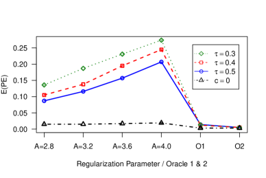
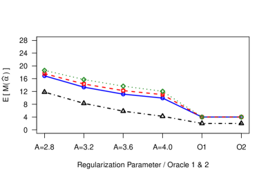
Figure 3. Mean Prediction Errors and Mean $\mathcal{M}(\widehat{\alpha})$ when $\rho=0.3$

$M=100$

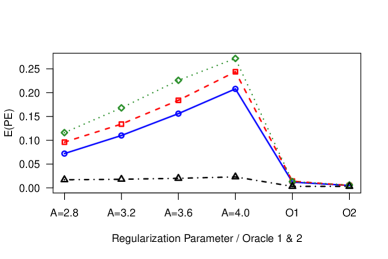
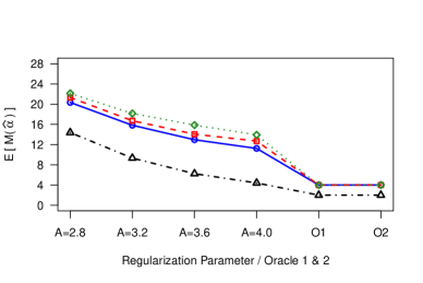
$M=200$

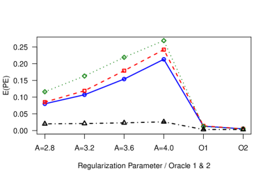
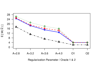
$M=400$

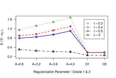
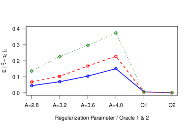
Figure 4. Mean $\ell_{1}$-Errors for $\alpha$ and $\tau$ when $\rho=0.3$

$M=100$

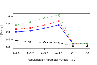
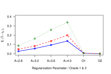
$M=200$

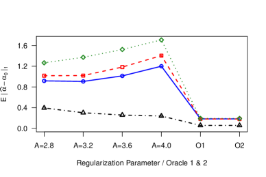
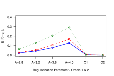
$M=400$

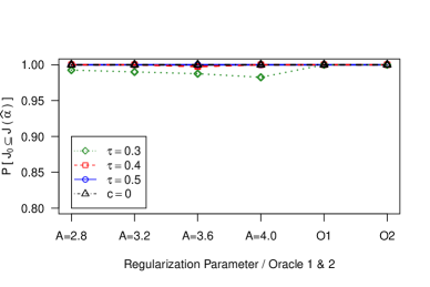
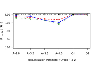
Figure 5. Probability of Selecting True Parameters when $\rho=0$ (left panel) and $\rho=0.3$ (right panel)

$M=50$

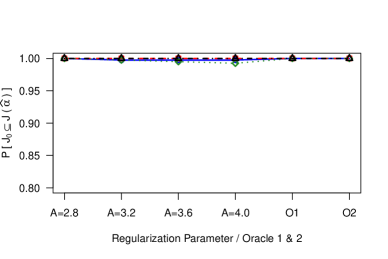
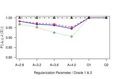
$M=100$

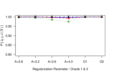
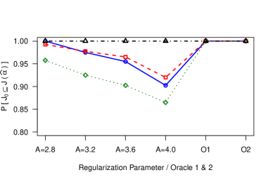
$M=200$

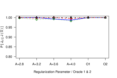
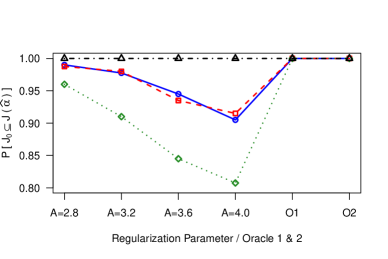
$M=400$