Collective effects in emission of quantum dots strongly coupled to a microcavity photon

Abstract

A theory of non-linear emission of quantum dot ensembles coupled to the optical mode of the microcavity is presented. Numerical results are compared with analytical approaches. The effects of exciton-exciton interaction within the quantum dots and with the reservoir formed by nonresonant pumping are considered. It is demonstrated, that the nonlinearity due to the interaction strongly affects the shape of the emission spectra. The collective superradiant mode of the excitons is shown to be stable against the non-linear effects.

1 Introduction

Semiconductor quantum dots are often referred to as “artificial atoms” owing to their discrete energy spectrum. The progress in nanotechnology has made it possible to employ quantum dots as a sui generis solid state laboratory for studies of quantum mechanics [1]. Interband optical pumping of quantum dots gives rise to the electron-hole pairs or zero-dimensional excitons, which, as shown in the pioneering works [2, 3, 4], can strongly couple with the photon trapped in the optical microcavity. The strong coupling effect results in a coherent energy transfer between the photon and the exciton, this phenomenon is widely studied for bulk materials and planar quantum well structures [5, 6, 7, 8]. Its observation in zero-dimensional systems has attracted an enormous excitement of the research community since the concepts of quantum electrodynamics were directly transferred to the solid state. Such quantum-dot-in-a-cavity systems demonstrate fascinating fundamental physics [9, 10, 11, 12] and may be advantageous for quantum optics device applications [13, 11, 14, 15].

The physical concept of the strong coupling in zero-dimensional microcavities can be easily understood considering, for the sake of an example, two classical pendulums with close frequencies of oscillations $\omega_{1}$ and $\omega_{2}$ connected by a spring, which induces the coupling between the pendulums of a strength $g$. One of these oscillators represents a photon, the other one stands for an exciton, and the spring describes radiative recombination of the exciton into the photon mode. If the dampings of the individual oscillators are small compared with the coupling constant, the eigenfrequencies $\omega$ of this interacting system follow from the simple equation

$$(\omega-\omega_{1})(\omega-\omega_{2})=g^{2}$$ (1)

as

$$\omega_{\pm}=\frac{\omega_{1}+\omega_{2}}{2}\pm\sqrt{\left(\frac{\omega_{1}-\omega_{2}}{2}\right)^{2}+g^{2}}.$$ (2)

The normal modes correspond to the coupled oscillations: By exciting one pendulum one eventually excites another, so the energy is transferred back and forth between them.

The analogy between the quantum electrodynamical problem of the quantum dot exciton interacting with the microcavity photon and purely classical problem of two coupled pendulums is quite deep. The excitonic polarization in a semiconductor is indeed described by the oscillator-like equation of motion and so does the electric field of the cavity photon [1, 7]. Hence, the physics of these two different systems is similar which greatly simplifies theoretical description of the quantum-dot-in-a-cavity dynamics [16, 17]. The situation becomes particularly interesting if $N>1$ dots are placed in the microcavity: It turns out that, provided the dots are identical, only one excitonic mode – termed superradiant – interacts with the cavity mode, and the interaction constant is enhanced compared with that in one dot by the factor $\sqrt{N}$. In classical language, for $N$ pendulums describing quantum dot excitons, one oscillation mode is specific, namely, the mode where all pendulums oscillate in phase with each other.

Just like the classical oscillators which are ideal only as far as model situations are considered, the excitons and photons interact with the environment, which gives rise to their damping and dephasing, moreover, the oscillation law can differ from the harmonic one. Main reasons of unharmonicity are identified: interactions between excitons lead to their energy shifts, the oscillator strength saturation results in the decrease of the coupling constant with an increase of the exciton number in the system, excitons can bind together to form biexcitons [1, 18]. Hence, the analysis of the non-linear dynamics of the quantum dot excitons strongly coupled to the cavity mode is of prime importance. In particular, the stability of the superradiant mode with respect to the interactions should be investigated.

In this paper, we consider the simplest possible and physically most transparent case of the non-linearity caused by the exciton-exciton interaction. It is analogous to the cubic unharmonicity of the pendulum. We calculate the optical emission spectra of the quantum-dot-in-a-cavity system under a non-resonant excitation (photoluminescence spectra). The non-resonant pumping is modeled as a random force acting on the corresponding oscillator [17, 22]. The parameter which controls the non-linearity is the pumping rate: the higher the pumping, the larger the fluctuations of excitonic polarization and, correspondingly, the higher are the non-linear terms in the equations of motion.

In our approach, the quantum dot state is described as a classical unharmonic oscillator. Hence, this approach is valid for large enough quantum dots where excitons are quantized as a whole. Similar behavior can be expected in a variety of systems including the semiconductor systems with planar quantum microcavities where excitons can be trapped by the disorder and the non-linear regime is easily reached [23, 24], or quantum well structures with dipolar excitons [25, 26], as well as many other, e.g. optomechanical structures where the optical mode of the cavity interacts with a classical oscillator [27].

The paper is organized as follows. Section 2 outlines the model, Sec. 3 is devoted to the role of the reservoir fluctuations, Sec. 4 presents the study of the nonlinearity due to the exciton interaction. Main results are summarized in Conclusions, Sec. 5.

2 Model

For distinctness we consider here a zero-dimensional microcavity where one or several quantum dots are embedded. We suppose that the energy (or frequency, we put $\hbar=1$ for brevity) spacing between the cavity modes is large enough to consider only one relevant photonic mode whose frequency $\omega_{C}$ is close enough to frequencies of optical transitions in quantum dots $\omega_{X,i}$, $i=1,\ldots,N$, where $N$ is the dot number. For simplicity, the interaction of the cavity mode with the ground states of quantum dot excitons is considered only, the treatment can be generalized to allow for the excited states. Moreover, the polarization degree of freedom of the cavity mode and spin degrees of freedom of excitons are disregarded. Under these approximations the equations of motion for the dimensionless electric field $E$ and excitonic polarizations $P_{i}$ can be written as

$$\frac{dE}{dt}=-\left(\rmi\omega_{C}+\frac{\Gamma_{C}}{2}\right)E-\rmi g\sum\limits_{i}P_{i}\>,$$ (3)

$$\frac{dP_{i}}{dt}=-\left(\rmi\omega_{X,i}+\frac{\Gamma_{X,i}}{2}+\rmi\alpha_{i}|P_{i}|^{2}+{\rmi\beta_{i}n_{R}}\right)P_{i}-\rmi gE+{f}_{i}(t),\quad i=1\ldots N\>.$$

Here $\Gamma_{C}$ and $\Gamma_{X,i}$ are (phenomenological) decay rates for the cavity and excitons, respectively, $g$ is the light-matter coupling constant (taken the same in all dots for the sake of simplicity). Its evaluation is beyond the current work, rigorously it can be done by solving Maxwell equations and Schrödinger equation for the exciton envelope functions in quantum dots, see Refs. [28, 29, 30].

Equation (3) for exciton polarization contains also non-linear and driving terms. Former ones, proportional to the interaction parameters $\alpha_{i}>0$, describe the blueshifts of excitonic states due to interactions within the same dot. Here and further we assume that the quantum dot size is comparable or larger than excitonic Bohr radius to accomodate several excitons in the dot [19]. Terms $\propto\beta_{i}n_{R}$ take into account the interaction of quantum dot excitons with a reservoir formed, e.g. by excitons and electron-hole pairs within the wetting layer. The reservoir population $n_{R}$ is, in general, function of the pumping intensity $W$ and exciton occupations, $n_{R}\equiv n_{R}(W,|P_{1}|^{2},\ldots,|P_{N}|^{2})$. Driving terms described by random forces $f_{i}$, $\langle f_{i}\rangle=0$ account for the exciton generation in quantum dots caused by their relaxation from the wetting layer and excited states, see Refs. [22, 17] for details. These random forces represent the white noise

$$\langle f_{i}(t)f_{j}^{*}(t^{\prime})\rangle=S_{i}\delta_{ij}\delta(t-t^{\prime})\>,$$ (4)

characterized by the exciton generation rate $S_{i}$ proportional to the reservoir population, $S_{i}=s_{i}n_{R}$, where $s_{i}$ is related with the relaxation rate of excitons towards the ground state [17]. In what follows we assume that higher-order correlators of random forces are reduced to the second order ones, Eq. (4), in accordance with the Gaussian distribution. Such random forces model the incoherent non-resonant pumping of our system. Similar approaches were used to study optical emission of exciton-polaritons in Bragg multiple quantum well structures and for planar microcavities [22, 32, 33, 34].

We are ultimately interested in the luminescence spectrum given (up to the common factor) by [17]:

$$I(\omega)=\langle|E(\omega)|^{2}\rangle=\int_{-\infty}^{\infty}\langle E(t+t^{\prime})E^{*}(t)\rangle e^{\rmi\omega t^{\prime}}\mathrm{d}t^{\prime},$$ (5)

where averaging over time $t$ is assumed. If the non-linear contributions are disregarded, emission spectrum can be obtained analytically with the result [17]:

$$I_{\rm lin}(\omega)=\sum\limits_{m,m^{\prime}=1}^{N+1}\frac{C^{(m)*}_{\rm cav}C^{(m^{\prime})}_{\rm cav}\sum_{i=1}^{N}C^{(m)*}_{i}S_{i}C^{(m^{\prime})}_{i}}{(\Omega_{m}^{*}-\omega)(\Omega_{m^{\prime}}-\omega)}\>.$$ (6)

Here, $\Omega_{m}$ are the eigenfrequencies of the homogeneous system (3) found neglecting non-linear terms $\propto\alpha_{i}$, $\beta$ i.e. $\Omega_{m}$ are the polariton frequencies, and $[C_{\rm cav}^{(m)},C_{1}^{(m)},...,C_{N}^{(m)}]\equiv[E,P_{1},\ldots,P_{N}]$ are the corresponding eigenvectors, i.e., the Hopfield coefficients of the excitonic polaritons formed by the excitons coupled to the cavity mode [7]. The spectrum Eq. (6) can also be recast as a sum of terms with poles at polariton frequencies $\Omega_{m}$, $\Omega_{m}^{*}$.

The detailed analysis of Eq. (6) is presented in Ref. [17]. Here we briefly discuss an important liming case where all exciton frequencies are the same, $\omega_{X,1}=\omega_{X,2}=\ldots=\omega_{X,N}\equiv\omega_{X}$, exciton decay rates are the same, $\Gamma_{X,1}=\Gamma_{X,2}=\ldots=\Gamma_{X,N}\equiv\Gamma_{X}$ and the decay rates are negligible compared with the coupling constants, $\Gamma_{X},\Gamma_{C}\ll g$. Under these assumptions the polariton frequencies and Hopfield coefficients take simple form. There are two mixed modes with the frequencies, cf. Eq. (2),

$$\Omega_{1,2}=\frac{\omega_{X}+\omega_{C}}{2}-\mathrm{i}\frac{\Gamma_{X}+\Gamma_{C}}{4}\pm\sqrt{\left(\frac{\omega_{X}-\omega_{C}}{2}\right)^{2}+Ng^{2}},$$ (7)

and all the remaining $N-1$ modes correspond to the exciton states decoupled from light, $\Omega_{m}=\omega_{X}$ for $m=3,\ldots N+1$. The effective coupling strength is enhanced by the factor $\sqrt{N}$ due to the superradiance effect: dipole moments of excitons oscillate in phase. Correspondingly, emission spectrum has two peaks at $\Omega_{1}$ and $\Omega_{2}$ splitted by $\sqrt{N}g$:

$$I_{\rm lin}(\omega)\equiv\langle|E(\omega)|^{2}\rangle\propto\frac{1}{|(\omega-\omega_{X}+\rmi\Gamma_{X}/2)(\omega-\omega_{C}+\rmi\Gamma_{C}/2)-Ng^{2}|^{2}}\>.$$ (8)

We note that Eq. (8) is valid even if the condition $\Gamma_{X}\ll g$ or $\Gamma_{C}\ll g$ is violated [17]. Two distinct peaks are observed in the emission spectra for the broadenings as high as $\Gamma_{X},\Gamma_{C}\sim\sqrt{N}g$, otherwise these two peaks merge into one.

Now we turn to the discussion of the non-linear effects. Firstly, we consider interactions with the reservoir described by the terms $\propto\beta_{i}n_{R}P_{i}$, afterwards we discuss the effects of exciton-exciton interaction within the same dot described by the terms $\propto\alpha_{i}|P_{i}|^{2}P_{i}$.

3 Interaction with reservoir

Under conventional non-resonant pumping conditions the excitons are generated in the wetting layer and form a reservoir. If the pumping rate is moderate the majority of excitons are in the reservoir and its occupation is only weakly affected by the presence of the quantum dots, hence, one can treat $n_{R}$ in Eqs. (3) as an independent quantity. For the steady-state pumping $\langle n_{R}\rangle=\bar{n}_{R}$ and there are certain fluctuations of $\delta n_{R}$ around this time-averaged value, $\delta n_{R}=n_{R}-\bar{n}_{R}$.

To elucidate the role of the reservoir we neglect completely the non-linearities caused by the exciton-exciton interaction in quantum dots, i.e. we put $\alpha_{i}\equiv 0$ in Eqs. (3). It is instructive to analyze the case of a single quantum dot and disregard the light-matter interaction. In this situation we obtain

$$\frac{dP}{dt}=-\left(\rmi\omega_{X}+\frac{\Gamma_{X}}{2}+\rmi\beta\bar{n}_{R}+\rmi\beta\delta n_{R}\right)P+f(t).$$ (9)

For clarity we have separated in Eq. (9) the contributions due to mean number of particles in reservoir and due to its fluctuations. Equation (9) is the first order linear differential equation which can be integrated with the result

$$P(t)=\int_{0}^{t}\mathrm{d}t^{\prime}f(t^{\prime})\exp{\left[-(\mathrm{i}\omega_{X}+\mathrm{i}\beta\bar{n}_{R}+\Gamma_{X}/2)(t-t^{\prime})-\mathrm{i}\beta\int_{t^{\prime}}^{t}\delta n_{R}(t^{\prime\prime})\rmd t^{\prime\prime}\right]},$$

where the solution of homogeneous equation is omitted. The autocorrelation function $\langle P(t)P^{*}(0)\rangle$, whose Fourier transform determines the single dot emission spectrum in the case of the regime of the weak coupling with the photon, reads

$$\langle P(t)P^{*}(0)\rangle=\frac{S}{\Gamma_{X}}\left\langle\exp{\left[-\mathrm{i}\omega_{X}t-\frac{\Gamma_{X}t}{2}-\rmi\beta\bar{n}_{R}t-\rmi\beta\int_{0}^{t}\delta n_{R}(t_{1})\mathrm{d}t_{1}\right]}\right\rangle.$$ (10)

Here the averaging over the random source realizations and reservoir population is assumed. The fluctuations of the reservoir particle number $n_{R}$ take place on much longer timescale compared with the fluctuations of random forces, Eq. (4). Hence, the averaging over the realizations of $f$ is carried out independently.

The oscillation spectrum, $\langle|P(\omega)|^{2}\rangle=\int_{-\infty}^{\infty}\langle P(t)P^{*}(0)\rangle\mathrm{d}t$, which corresponds to the quantum dot emission spectrum in the weak coupling regime, depends strongly on the relation between various timescales in the system: exciton lifetime $1/\Gamma_{X}$, correlation time in the reservoir $\tau_{c}$, defined by the relation $\langle\delta n_{R}(t)\delta n_{R}(0)\rangle=\langle\delta n_{R}^{2}\rangle\rme^{-t/\tau_{c}}$, and dephasing time $\tau_{d}$ caused by the reservoir, where

$$\frac{1}{\tau_{d}}=\beta^{2}\int_{0}^{\infty}\mathrm{d}t\,\langle\delta n_{R}(t)\delta n_{R}(0)\rangle=\beta^{2}\langle\delta n_{R}^{2}\rangle\tau_{c}.$$ (11)

If reservoir fluctuations are fast and small enough, $\tau_{c}\ll\tau_{d}$, $\Gamma_{X}^{-1}$, the so-called motional narrowing regime can be realized and

$$\langle|P^{2}(\omega)|\rangle\propto\frac{1}{(\omega-\omega_{X}-\beta\bar{n}_{R})^{2}+[\Gamma_{X}/2+1/(2\tau_{d})]^{2}}.$$ (12)

In this case interactions with reservoir slightly broaden the quantum dot spectrum.

In the opposite case, where the fluctuations are strong and slow, the quantum dot spectrum can be presented as

$$\langle|P(\omega)|^{2}\rangle\propto{\int\mathrm{d}n_{R}\,p(n_{R})\delta(\omega-\omega_{X}-\beta n_{R})=\frac{1}{\beta}p\left(\frac{\omega-\omega_{X}}{\beta}\right),}$$ (13)

where $p(n_{R})$ is the distribution function of the reservoir, i.e. the probability that the number of particles in the reservoir is $n_{R}$. The quantum dot spectrum Eq. (13) in the regime of strong fluctuations is strongly asymmetric and reflects the distribution of the particles in the reservoir. Equation (13) is valid for the frequencies $|\omega-\omega_{X}-\beta\bar{n}_{R}|\gtrsim\Gamma_{X}$, that is why the spectral function of the quantum dot is replaced by $\delta$-function in Eq. (13). This equation also holds provided that the particle number fluctuations in the reservoir are so large that

$$\beta\sqrt{\langle\delta n_{R}^{2}\rangle}\gg\Gamma_{X},\tau_{c}^{-1}.$$ (14)

In this case the dephasing takes place at a timescale $\sim(\beta\sqrt{\langle\delta n_{R}^{2}\rangle})^{-1}$ and it is not sensitive neither to the oscillator lifetime nor to the correlation time of the reservoir.

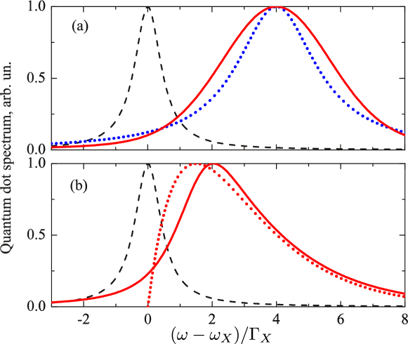
Figure 1: (Color online) Effect of interaction with the reservoir (a) and within the quantum dot (b) on its spectrum $\langle|P(\omega)|^{2}\rangle$. Black/dashed, red/solid and blue/dotted curves in panel (a) correspond to linear regime, fast reservoir fluctuations regime and regime of slow reservoir fluctuations with Gaussian statistics, respectively. Calculation was performed at $\beta\bar{n}_{R}=4\Gamma_{X}$, $1/\tau_{d}=2\Gamma_{X}$ and $\beta\delta\bar{n}_{R}=1.5\Gamma_{X}$. Black/dashed, red/solid and red/dotted curves in panel (b) correspond to linear regime, exact solution, Eq. (23), and approximate solution Eq. (22), with $\delta$-function replaced by Lorentzian with full-width at half-maximum equal to $\Gamma_{X}$. Calculation was performed at $\alpha S=3\Gamma_{X}$.

These two limiting cases of reservoir fluctuations described by Eqs. (12) and (13) are illustrated in Fig. 1(a) where the calculated quantum dot spectra are shown. Black/dashed curve presents spectrum for vanishing reservoir fluctuations, this spectrum is described by the Lorentzian with the full width at half-maximum (FWHM) equal to $\Gamma_{X}$, centered at the resonance frequency $\omega_{X}$. Blue/dotted curve corresponds to the regime of fast reservoir fluctuations, Eq. (12). This spectrum is also a Lorentzian, shifted to larger energies and broadened as compared to the linear regime. Red/solid curve is calculated in the regime of slow reservoir fluctuations. We have assumed, that the reservoir population is characterized by a Gaussian distribution with given mean value $\bar{n}_{R}$ and dispersion $\delta n_{R}$. In numerical calculations the $\delta$-function in Eq. (13) was replaced by the Lorentzian with FWHM equal to $\Gamma_{X}$. Then the convolution (13) yields Voigt distribution with Gaussian-like central part and Lorentzian wings, see Fig. 1(a).

It is noteworthy that for the quantum dot placed into the microcavity, the emission spectrum in the limit of weak and fast fluctuations, $\tau_{c}\ll\tau_{d},\Gamma_{X}^{-1}$ is given by Eq. (6) where $\omega_{X}$ is replaced by $\omega_{x}+\beta\bar{n}_{R}$ and $\Gamma_{X}$ is replaced by $\Gamma_{X}+\tau_{d}^{-1}$. The qualitative shape of the spectra in the case of strong or slow reservoir fluctuations can be obtained by the convolution of the reservoir distribution function $p(n_{R})$ with Eq. (6) where $\omega_{X}$ is substituted by $\omega_{X}+\beta n_{R}$. The resulting spectra are similar to those discussed in Sec. 4.2 where the case of the nonlinearity within the dot is addressed.

4 Interaction within the dot

Now we focus on the non-linear effects due to the interaction of the excitons within the same quantum dot. Hereinafter we disregard fluctuations of the particles in the reservoir studied above in Sec. 3. Below we present one after another the studies of (i) the single dot case (Sec. 4.1), (ii) the single dot coupled with the cavity mode (Sec. 4.2), and (iii) two quantum dots coupled with the cavity (Sec. 4.3).

4.1 Single dot

The physical picture of the interaction effects within the dot on the emission spectra can be most transparently presented for the case of the single quantum dot which does not interact with the photon. Similarly to the situation studied in Sec. 3 its spectral function $\langle|P(\omega)|^{2}\rangle$ defines the emission spectrum in the weak coupling regime.

We start with the equation describing quantum dot as a non-linear oscillator:

$$\frac{dP}{dt}=-\left(\rmi\omega_{X}+\rmi\alpha|P|^{2}+\frac{\Gamma_{X}}{2}\right)P+f(t)\>,\quad\langle f(t)f^{*}(t^{\prime})\rangle=S\delta(t-t^{\prime})\>.$$ (15)

Similarly to the case of reservoir fluctuations, Eq. (9), the interaction term in Eq. (15) leads to the blueshift and broadening of the oscillation spectrum. Consequently, the analysis of reservoir fluctuations, performed above, may be used here. The strength of the fluctuating non-linear term is determined by the value of pumping. Large pumping ($\alpha\langle|P|^{2}\rangle\gg\Gamma_{X}$) corresponds to the regime of strong fluctuations, cf. Eq. (14). Hence, the quantum dot spectrum may be presented in the form, similar to Eq. (13),

$$\langle|P(\omega)|^{2}\rangle=\int\rmd\Omega F(\Omega)\delta(\Omega-\omega)\>,$$ (16)

where the distribution function $F(\Omega)$ with the oscillator frequency $\Omega=\omega_{X}+\alpha|P|^{2}$, is determined from the statistics of the non-linear term in Eq. (15).

The major difference of the non-linear Eq. (15) and the linear one Eq. (9) describing the interaction of the quantum dot exciton with the reservoir is that the fluctuations of the polarization $P$ themselves govern the blueshift and, on the other hand, the blueshift determines the fluctuations of $P$. In order to determine the distribution function $F(\Omega)$ we use the stochastic linearization of Eq. (15) described in detail in Refs. [35, 36]. The starting point of the stochastic linearization is the time-dependent Eq. (15) where decay and pumping terms are neglected, $\Gamma_{X}\equiv 0$, $f(t)\equiv 0$. The solution of Eq. (15) is then given by $P(t)=|P|\rme^{-\rmi\Omega t}$, where

$$\Omega|P|^{2}=\omega_{X}|P|^{2}+\alpha|P|^{4}\>.$$ (17)

In the presence of the decay and pumping Eq. (17) does not hold. In the stochastic linearization approach the difference of the left- and right- hand sides of Eq. (17) should be minimized. It implies, in particular, that the average (over the random sources realizations) blueshift of the resonance frequency is given by

$$\langle\Omega-\omega_{X}\rangle=\frac{\alpha\langle|P|^{4}\rangle}{\langle|P|^{2}\rangle}\>.$$ (18)

Hereinafter we use the notation $\langle|P|^{2}\rangle\equiv\langle|P(t=0)|^{2}\rangle=\int\rmd\omega\langle|P(\omega)^{2}|\rangle/(2\pi)$. Equation (18) is automatically satisfied when the distribution of the frequency $\Omega$ is chosen in the form

$$F(\Omega)=\mathcal{N}(\Omega-\omega_{X})p\left(\frac{\Omega-\omega_{X}}{\alpha}\right)\>,$$ (19)

where $\mathcal{N}$ is the normalization constant,

$$p(|P|^{2})=\frac{1}{\langle|P|^{2}\rangle}\exp\left(-\frac{|P|^{2}}{\langle|P|^{2}\rangle}\right)\>,$$ (20)

is the distribution function of the exciton polarization absolute value, and

$$\langle|P^{2}|\rangle=\frac{S}{\Gamma_{X}}\>,$$ (21)

is given by the ratio of the pumping and decay rates. The shape of this distribution is independent of the pumping rate. In other words, the non-linear term in Eq. (15) influences the oscillator phase only and does not affect its amplitude. Thus, the distribution Eq. (20) is the same as in the linear regime and it inherits the Gaussian statistics of the noise term fluctuations. Using Eq. (18) and Eq. (20) we find that

$$\langle|P(\omega)|^{2}\rangle\propto F(\omega)=\cases{(\omega-\omega_{X})\exp\left(-\frac{\omega-\omega_{X}}{\alpha\langle|P^{2}|\rangle}\right),&$\omega>\omega_{X}$\cr 0,&$\omega<\omega_{X}$.}$$ (22)

This function decays exponentially for large values of $\Omega$ because the realization of high blueshift $\alpha|P^{2}|$ is unlikely. Moreover, frequencies $\omega<\omega_{X}$ are not possible since interactions are repulsive and lead to the increase of energy only. Equation (22) demonstrates, that in the regime of high pumping the oscillator spectrum is strongly asymmetric and broadened due to the fluctuations of the resonance frequency.

For arbitrary value of pumping strength the general analytical result for the oscillator spectrum can be obtained by means of the Fokker-Planck equation technique [37, 21], similarly to the case of the noise-driven Duffing oscillator [38]. The spectrum reads

$$\langle|P(\omega)^{2}|\rangle\propto\mathop{\mathrm{Im}}\nolimits\sum\limits_{n=0}^{\infty}\frac{(I_{n})^{2}}{\lambda_{n}-\omega}\>,$$ (23)

where

$$\lambda_{n}=\omega_{X}+\rmi\frac{\Gamma_{X}}{2}-2\rmi(n+1)\sqrt{\left(\frac{\Gamma_{X}}{2}\right)^{2}+\rmi\alpha S}\>,$$

$$I_{n}=\frac{4b\sqrt{(n+1)a}}{(a+b)^{2}}\left(\frac{a-b}{a+b}\right)^{n},\quad a=\frac{\Gamma_{X}}{S},\quad b=\sqrt{a^{2}+\frac{4\rmi\alpha}{S}}\>.$$

In the linear in the pumping regime where $S\to 0$ only the first term in the series Eq. (23) does not vanish and the result is reduced to Lorentzian with FHWM equal to $\Gamma_{X}$. For very large pumping, $\alpha\langle|P^{2}|\rangle\gg\Gamma_{X}$, the series reduce to Eq. (22).

The spectra of the single oscillator, $\langle|P(\omega)|^{2}\rangle$, calculated for different pumping strengths, are shown in Fig. 1(b). The spectrum at the strong pumping represented by red/solid curve, is strongly broadened and shifted as compared to the spectrum found in the linear regime. The latter is shown by black/dashed black curve. The width of the non-linear spectrum is of the same order as the blueshift. The spectrum found by the stochastic linearization, Eq. (22), and shown by red/dotted curve in Fig. 1(b) well approximates the exactly calculated one, Eq. (23). The strong asymmetry of emission spectra calculated for the non-linear regime is clearly seen from the Figure.

This concludes the discussion of the single oscillator and now we proceed to the analysis of the quantum dot coupled with the cavity mode.

4.2 Single dot coupled with the cavity

To start, we recall that in the linear-in pumping regime, $S\to 0$, and under the conditions of the strong coupling, $g\gg\Gamma_{C},\Gamma_{X}$, the spectrum described by Eq. (8) with $N=1$ consists of the two distinct peaks at the frequencies of the system eigenmodes, excitonic polaritons. The main question we address here is how this two-peak spectrum changes with allowance for the non-linearity. In the general case the emission spectrum under strong pumping should be calculated numerically. This can be done either reducing the problem to the Fokker-Planck equation [37] or directly integrating the set of Eqs. (3). The latter procedure turns out to be more efficient, because the Fokker-Planck equation is computationally demanding already for $N=1$ due to the large number of independent variables. In our calculations we have used the simplest 1.5-order Heun method for integration of stochastic differential equations [39, 40].

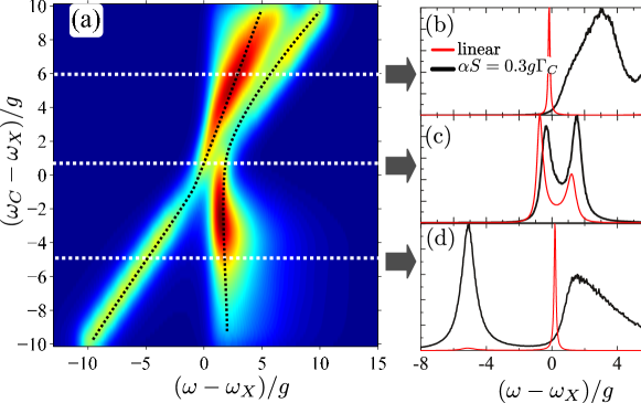
Figure 2: (Color online) (a) Photoluminescence spectra for single quantum dot coupled to microcavity mode as function of the detuning between cavity and exciton frequencies. Panels (b),(c),(d) show the spectra for $\omega_{C}=\omega_{X}+6g$, $\omega_{C}=\omega_{X}+0.5g$, $\omega_{C}=\omega_{X}-5g$, respectively. Black/thick and red/thin lines in panels (b), (c), and (d) correspond to non-linear and linear in pumping regime, $\alpha S=0.3g\Gamma_{C}$ and $S=0$, respectively. These curves are normalized to their maximum values. Black/dashed curves in panel (a) are guides for eye demonstrating anticrossing. Calculations are carried out at $\Gamma_{X}=0.1g$, $\Gamma_{C}=g$, $\alpha S=0.3g\Gamma_{C}$. The time-domain integration was performed up to $t=100/g$, with the time step $0.003/g$, the spectra were averaged over ensemble with $4000$ realizations of random forces.

Luminescence spectra calculated for different detunings between the exciton and photon modes are presented in Fig. 2. Panel (a) shows the color plot of the emission intensity. Panels (b), (c), and (d) present the spectra for the detuning $\omega_{C}-\omega_{X}$ equal to $6g$, $0.5g$ and $-5g$, respectively. Thin/red and thick/black curves are calculated, respectively, for (i) the linear regime $S\to 0$ and (ii) the regime where the non-linearity is already strong, $S=0.3\Gamma_{C}/\alpha$. The spectra are normalized to their maximum values, the other parameters of the calculations are given in the caption to the Figure. The calculation demonstrates, that the non-linear spectra retain the characteristic two-peak structure, although the spectral shape is strongly affected by the non-linearity, in particular, it becomes asymmetric, as well seen in Figs. 2(b) and (d). The spectral maxima in the non-linear regime clearly exhibit the anticrossing behavior, see Fig. 2(a). From this we conclude that the strong coupling survives even for non-linear regime if $\alpha\langle|P^{2}|\rangle\lesssim g$.

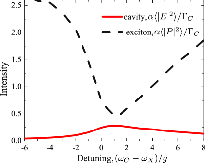
Figure 3: (Color online) Intensities of photon and exciton modes as functions of the detuning $\omega_{C}-\omega_{X}$. Red/solid and black/dashed curves correspond to $\alpha\langle|E|^{2}\rangle/\Gamma_{C}$ and $\alpha\langle|P|^{2}\rangle/\Gamma_{C}$, respectively. The parameters of calculations are the same as in Fig. 2.

Let us now discuss the spectra in Fig. 2 in more detail. We start from the case of large detuning between exciton and photon modes, $|\omega_{X}-\omega_{C}|\gg g$. In this situation the spectrum has two peaks related with the cavity and exciton emission. It is noteworthy, that in the non-linear regime, the blueshift of the exciton is determined by the dot population which, in its turn, is related with the detuning: $\langle|P|^{2}\rangle\approx S(\omega_{X}-\omega_{C})^{2}/(\Gamma_{C}g^{2})$ (provided that $\Gamma_{X}\ll\Gamma_{C}$ and $\Gamma_{C}\ll|\omega_{X}-\omega_{C}|$). Hence, if bare exciton frequency $\omega_{X}$ is fixed, but the cavity frequency $\omega_{C}$ is varied, the position of exciton peak changes due to the variation of the blueshift.

To confirm this argument we have plotted in Fig. 3 the dependence of the stationary intensities $\langle|E|^{2}\rangle$ and $\langle|P^{2}|\rangle$ on the detuning. For large detuning one has $\langle|P^{2}|\rangle\gg\langle|E|^{2}\rangle$ which is explained by the longer exciton lifetime as compared to the photon lifetime, $\Gamma_{C}\gg\Gamma_{X}$. For small values of detuning the curves become closer to each other as a result of the coupling between exciton and photon modes.

Another important feature revealed in Fig. 2 is the strong asymmetry between the spectral shapes of the exciton peak for large positive and negative detuning, cf. Fig. 2(b) and Fig. 2(c). This is quite different from the linear regime, where the spectra Eq. (8) are symmetric with respect to zero detuning. In the non-linear case the exciton peak is asymmetrically broadened due to the frequency fluctuations, like in the case of single oscillator, and the shape of the broadened peak depends on the sign of detuning. For negative detuning, $\omega_{C}-\omega_{X}<0$, the high-energy tail dominates the spectrum similarly to the case of the dot decoupled from the cavity, see Sec. 4.1 and Fig. 1(b), while for positive detuning, $\omega_{C}-\omega_{X}>0$, this tail is quenched. This is related with the fact that strong fluctuations of exciton polarization $P$ are strongly suppressed since they correspond to large blueshifts where exciton mode approaches the cavity mode and, hence, short lifetimes.

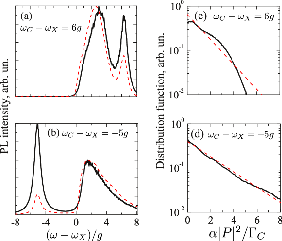
Figure 4: (a), (b) Cavity emission spectra calculated for the detuning $\omega_{C}-\omega_{X}=6g$ (a), and $\omega_{C}-\omega_{X}=-5g$ (b). (c), (d) Distribution functions of the intensity $|P|^{2}$ calculated for the same parameters as in panels (a) and (b), respectively. Black/solid lines represent results of direct numerical calculation, red/dashed lines are calculated according to Eqs. (20),(24). Other parameters of calculations are the same as in Fig. 2.

To understand this effect in depth we have plotted in Fig. 4 the emission spectra [(a), (b)] along with the distribution functions of the quantum dot exciton intensity $|P|^{2}$. Distribution functions $p(|P|^{2})$, shown by black/solid curves in Fig. 4(c) and Fig. 4(d), were extracted from the numerical solutions of the system (8). For comparison, red/dashed curves show exponential distributions (20) with the same average values of $|P|^{2}$. The emission spectrum of the microcavity can be presented in the following phenomenological form similar to Eq. (13) and Eq. (16) obtained in the stochastic linearization method:

$$I(\omega)\propto\int\rmd\Omega F(\Omega)I_{\rm lin}(\omega)\>.$$ (24)

where $I_{\rm lin}(\omega)$ is given by Eq. (8) with $\omega_{X}=\Omega$ and the distributions $F(\Omega)$ and $p(|P^{2}|)$ are related by Eq. (18). Corresponding spectra, calculated with numerically found functions $p(|P|^{2})$, are shown in Fig. 4(a) and Fig. 4(b) by red/thin curves. We see, that Eq. (24) satisfactory describes the shape of the exciton peaks for both signs of the detuning and clearly demonstrates the correspondence between the shape of the exciton peak and the distribution function of the intensity $|P|^{2}$. For negative detuning the distribution function and the excitonic peak have exponential tails, similarly to the case of single oscillator, Eq. (22). Suppression of this tail for positive detuning means that the distribution function decays faster than exponential [cf. red and black curves in Fig. 4(c)] which is explained by interaction of excitonic and photonic modes. Indeed, for $\omega_{C}>\omega_{X}$ the non-linear blueshift of the exciton frequency decreases the detuning. Consequently, the exciton lifetime becomes effectively smaller due to the Purcell effect which suppresses the probability of such large detuning. Another effect leading to the same result is the repulsion of the excitonic mode with high blueshift from the cavity mode. In the opposite case, $\omega_{C}<\omega_{X}$, the absolute value of the detuning is further increased by the blueshift, so the shape of the excitonic peak is not modified by the interaction with the cavity.

Phenomenological Eq. (24) fails, however, to reproduce the ratio between the magnitudes of the excitonic and photonic peaks in the spectra. Formally, Eq. (24) is valid provided that the timescale of the fluctuations of $P$ is large compared with other timescales in the system [cf. Eq. (14)] or the magnitude of the blueshift exceeds by far all other energy scales. Neither of these conditions holds in the system under study.

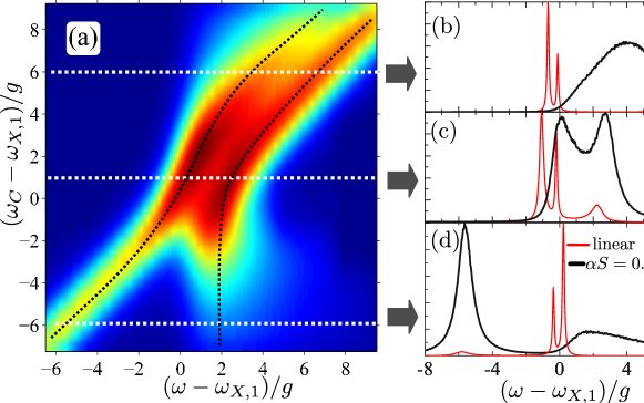
Figure 5: (a) Photoluminescence spectra for two quantum dots coupled to microcavity mode as function of the detuning between cavity and exciton dot. Panels (b), (c), (d) show the spectra for $\omega_{C}=\omega_{X,1}+6g$, $\omega_{C}=\omega_{X}+g$, $\omega_{C}=\omega_{X}-6g$, respectively. Black/thick and red/thin lines in panels (b) – (d) correspond to non-linear and linear in pumping regime, $\alpha S=0.4g\Gamma_{C}$ and $S\to 0$, respectively. These curves are normalized at their maximum values. Black/dashed curves in panel (a) are guides for eye demonstrating anticrossing. Calculation was carried out for $\omega_{X,1}-\omega_{X,2}=g$, other parameters are the same as in Fig. 2.

4.3 Two dots coupled with the cavity

Now we turn to the discussion of the emission spectra of the cavity with two embedded dots, shown in Fig. 5. The specific feature of this problem in the linear regime is the formation of the collective, superradiant mode of the quantum dot excitons [16, 17, 21]. In particular, as discussed above in Sec. 2, there are three eigenmodes of the homogeneous linear system Eq. (3) for $N=2$. In case where $\omega_{X,i}=\omega_{X,2}$, one of these modes, with the excitons oscillating with the opposite phases, $P_{1}=-P_{2}$, does not interact with the cavity mode, it is called dark. Two remaining modes correspond to the excitons, oscillating in phase, $P_{1}=P_{2}$, and are formed by the coupling between the superradiant mode of the excitons and the cavity mode. Only two peaks are manifested in the emission spectrum. The superradiant effect leads to the enhancement of the Rabi splitting between these peaks from $g$ to $\sqrt{N}g$, see Eq. (8). When the frequencies of the dots $\omega_{X,i}$ are different, or the exciton tunneling between the dots is introduced, the dark modes mix with the superradiant mode and the spectrum acquires three-peak shape. As is demonstrated in previous work [17], the superradiant mode is stable against the disorder when the characteristic splitting of the dot frequencies is less than $g\sqrt{N}$. Here we analyze the stability of the superradiant mode against the interactions.

Figure 5 shows the emission spectra of the microcavity containing two quantum dots for various frequencies of the cavity mode. The frequency separation between the dots was fixed to be $\omega_{X,2}-\omega_{X,1}=g$ and the $\omega_{C}$ was varied. Overall intensity dependence on the emission and cavity frequency shown in Fig. 5(a) is quite similar to the intensity distribution for one dot in the microcavity [see Fig. 2(a)] and clearly demonstrates two peaks for any given cavity mode position. Thus, the superradiant mode is stable against the interaction.

Panels (b), (c), and (d) of Fig. 5 present the details of emission spectra for three different cavity mode positions. Black/solid curves are calculated for the strong pumping where the nonlinear behavior is pronounced, red/thin curves correspond to the linear regime. The emission spectra in the non-linear regime corresponding to rather large detunings [panels (b), (d)] demonstrate the asymmetry studied for the single dot in the cavity in Sec. 4.2. Interestingly, the spectra in the linear regime demonstrate three peaks: two stronger ones correspond to the dot emission and weaker one to the cavity emission. The presence of non-linearity induced by the strong pumping qualitatively changes the emission spectrum: excitonic peaks merge and their intensity drops. Note, however, that the strong coupling regime is still maintained, see anticrossing in Fig. 5. The smallest splitting between the maxima of the spectra is larger than the Rabi splitting for the single dot $2g$. This is a fingerprint of the superradiant mode stability in the non-linear regime.

Thus, the superradiant mode becomes stabilized by interactions. Indeed, for positive detunings, $\omega_{C}>\omega_{X,1},\omega_{X,2}$, the blueshifts of the quantum dots are different: The dot with higher exciton frequency (dot 2 in our calculation) has smaller lifetime due to proximity to the cavity mode, correspondingly, smaller exciton intensity $\langle|P_{2}|^{2}\rangle<\langle|P_{1}|^{2}\rangle$, and, hence, smaller blueshift. Hence, with an increase of the pumping rate the blueshifted dot frequencies approach to each other, resulting in the decrease of the splitting between exciton frequencies and stabilization of the superradiant mode.

5 Conclusions

To conclude, we have developed a theory of non-linear emission of quantum dots coupled to the optical mode of the microcavity under non-resonant excitation. We model quantum dot excitons as non-linear oscillators taking into account the repulsive exciton-exciton interactions both within the dot and between the quantum dot and excitonic reservoir. We use random sources approach to model the relaxation processes and apply stochastic linearization and numerical integration of the Langevin equations to determine the spectra.

Our model clearly shows that interactions: (i) blueshift the transition energy and (ii) to the same extent broaden the emission peak. The interactions result in the complex behavior of the exciton lifetimes and intensities of emission as functions of pumping rate. The emission lines are strongly asymmetric and bear information on the exciton statistics. Contrary to the linear regime, the lineshapes are sensitive to the sign of the detuning between the exciton and photon modes. Interestingly, even for substantial pumping the strong coupling regime between the cavity mode and the quantum dot exciton can be preserved. Moreover, if two quantum dots are placed in the cavity, the superradiant behavior can be stabilized by the pumping.

References

- [1] Ivchenko E L 2005 Optical spectroscopy of semiconductor nanostructures (Harrow, UK: Alpha Science International)
- [2] Reithmaier J P, Sek G, Löffler A, Hofmann C, Kuhn S, Reitzenstein S, Keldysh L V, Kulakovskii V D, Reinecke T L and Forchel A 2004 Nature 432 197
- [3] Yoshie T, Scherer A, Hendrickson J, Khitrova G, Gibbs H M, Rupper G, Ell C, Shchekin O B and Deppe D G 2004 Nature 432 200
- [4] Peter E, Senellart P, Martrou D, Lemaitre A, Hours J, Gérard J M and Bloch J 2005 Phys. Rev. Lett. 95 067401
- [5] Agranovich V and Ginzburg V 1984 Crystal optics with spatial dispersion, and excitons: Springer series in solid-state sciences (Springer-Verlag)
- [6] Kavokin A and Malpuech G 2003 Cavity Polaritons (Amsterdam: Elsevier)
- [7] Kavokin A, Baumberg J, Malpuech G and Laussy F 2006 Microcavities (Oxford: Clarendon Press)
- [8] Rashba E and Sturge M (eds) 1982 Excitons (Modern Problems in Condensed Matter Science vol 2) (Amsterdam: North-Holland)
- [9] Khitrova G, Gibbs H M, Kira M, Koch S W and Scherer A 2006 Nature Physics 2 81
- [10] Kasprzak J, Reitzenstein S, Muljarov E A, Kistner C, Schneider C, Strauss M, Höfling S, Forchel A and Langbein W 2010 Nature Materials 9 304
- [11] Nomura M, Kumagai N, Iwamoto S, Ota Y and Arakawa Y 2010 Nature Physics 6 279–283
- [12] Calic M, Gallo P, Felici M, Atlasov K A, Dwir B, Rudra A, Biasiol G, Sorba L, Tarel G, Savona V and Kapon E 2011 Phys. Rev. Lett. 106 227402
- [13] Dousse A, Suffczynski J, Beveratos A, Krebs O, Lemaitre A, Sagnes I, Bloch J, Voisin P and Senellart P 2010 Nature 466 217
- [14] Ota Y, Iwamoto S, Kumagai N and Arakawa Y 2011 Phys. Rev. Lett. 107(23) 233602
- [15] Tandaechanurat A, Ishida S, Guimard D, Nomura M, Iwamoto S and Arakawa Y 2011 Nature Photonics 5 91–94
- [16] Keldysh L V, Kulakovskii V D, Reitzenstein S, Makhonin M N and Forchel A 2007 JETP lett. 84 494
- [17] Averkiev N S, Glazov M M and Poddubnyi A N 2009 JETP 108 836
- [18] Khitrova G, Gibbs H M, Jahnke F, Kira M and Koch S W 1999 Rev. Mod. Phys. 71(5) 1591–1639
- [19] Laussy F P, Glazov M M, Kavokin A, Whittaker D M and Malpuech G 2006 Phys. Rev. B 73 115343 (pages 13)
- [20] del Valle E, Laussy F P and Tejedor C 2009 Phys. Rev. B 79 235326
- [21] Poddubny A N, Glazov M M and Averkiev N S 2010 Phys. Rev. B 82 205330
- [22] Deych L I, Erementchouk M V, Lisyansky A A, Ivchenko E L and Voronov M M 2007 Phys. Rev. B 76 075350
- [23] Kasprzak J, Richard M, Kundermann S, Baas A, Jeambrun P, Keeling J M J, Marchetti F M, Szymanska M H, André R, Staehli J L, Savona V, Littlewood P B, Deveaud B and Dang L S 2006 Nature 443 409
- [24] Malpuech G, Solnyshkov D D, Ouerdane H, Glazov M M and Shelykh I 2007 Phys. Rev. Lett. 98 206402
- [25] Butov L V, Lai C W, Ivanov A L, Gossard A C and Chemla D S 2002 Nature 417 47
- [26] Timofeev V B, Gorbunov A V and Demin D A 2011 Low Temperature Physics 37 179
- [27] Aspelmeyer M, Gröblacher S, Hammerer K and Kiesel N 2010 J. Opt. Soc. Am. B 27 A189
- [28] Andreani L C, Panzarini G and Gérard J M 1999 Phys. Rev. B 60 13276
- [29] Kaliteevski M A, Brand S, Abram R A, Nikolaev V V, Maximov M V, Sotomayor Torres C M and Kavokin A V 2001 Phys. Rev. B 64 115305
- [30] Glazov M, Ivchenko E, Poddubny A and Khitrova G 2011 Phys. Solid State 53 1753
- [31] Tosi G, Christmann G, Berloff N G, Tsotsis P, Gao T, Hatzopoulos Z, Savvidis P G and Baumberg J J 2012 Nature Physics 8 190–194
- [32] Wouters M and Savona V 2009 Phys. Rev. B 79 165302
- [33] Sarchi D, Wouters M and Savona V 2009 Phys. Rev. B 79 165315
- [34] Wouters M and Savona V 2010 Phys. Rev. B 81 054508
- [35] Budgor A B 1976 J. Statistical Phys. 15 355
- [36] Spanos P, Kougioumtzoglou I and Soize C 2011 Probabilistic Engineering Mechanics 26 10
- [37] Risken H 1989 The Fokker-Planck Equation. Methods of Solution and Applications (Berlin: Springer)
- [38] Dykman M I and Krivoglaz M A 1980 Physica A 104 495–508
- [39] Kloeden P and Platen E 2010 Numerical Solution of Stochastic Differential Equations Stochastic Modelling and Applied Probability (Springer)
- [40] Burrage K, Lenane I and Lythe G 2007 SIAM Journal on Scientific Computing 29 245