Indirect Probes of Supersymmetry Breaking in the JEM-EUSO Observatory

Abstract

In this paper we propose indirect probes of the scale of supersymmetry breaking, through observations in the Extreme Universe Space Observatory onboard Japanese Experiment Module (JEM-EUSO). We consider scenarios where the lightest supersymmetric particle is the gravitino, and the next to lightest (NLSP) is a long lived slepton. We demonstrate that JEM-EUSO will be able to probe models where the NLSP decays, therefore probing supersymmetric breaking scales below $5\times 10^{6}$ GeV. The observatory field of view will be large enough to detect a few tens of events per year, depending on its energy threshold. This is complementary to a previous proposal abc where it was shown that 1 Km³ neutrino telescopes can directly probe this scale. NLSPs will be produced by the interaction of high energy neutrinos in the Earth. Here we investigate scenarios where they subsequently decay, either in the atmosphere after escaping the Earth or right before leaving the Earth, producing taus. These can be detected by JEM-EUSO and have two distinctive signatures: one, they are produced in the Earth and go upwards in the atmosphere, which allows discrimination from atmospheric taus and, second, as NLSPs are always produced in pairs, coincident taus will be a strong signature for these events. Assuming that the neutrino flux is equivalent to the Waxman-Bahcall limit, we determine the rate of taus from NLSP decays reaching JEM-EUSO’s field of view.

I Introduction

Probes of the origin and stability of the weak scale and proposed solutions to the standard model hierarchy problem is now underway at the Large Hadron Collider (LHC). On the theoretical side, the supersymmetric theory (Susy) arises as a solution with no significant deviation from the standard model (SM) in relation to electroweak precision observables. It has been shown abc ; abcd that neutrino telescopes can probe the scale of supersymmetry breaking ($\sqrt{F}$) or of Universal Extra Dimensions scenarios abckk . While R parity symmetry ensures that the lightest supersymmetric particle (LSP) is stable, the identity of the LSP is determined by $\sqrt{F}$. If Susy is broken at $\sqrt{F}>10^{10}$ GeV the LSP is typically the neutralino, if $\sqrt{F}<10^{10}$ GeV it is typically the gravitino.

There are many Susy scenarios where $\sqrt{F}$ is low, among which Gauge Mediation Susy Breaking models gmsb . In these scenarios the NLSP is a charged slepton, typically a right-handed stau, and it’s lifetime is given by abc :

$$c\tau=\left(\frac{\sqrt{F}}{10^{7}{\rm~{}GeV}}\right)^{4}\,\left(\frac{100~{}{\rm GeV}}{m_{\tilde{\tau}}}\right)^{5}\,10~{}{\rm km}~{},$$ (1)

where ${m_{\tilde{\tau}}}$ is the stau mass. It was shown abc ; abcd that Km³ neutrino telescopes can directly probe the Susy breaking scale, when one consider scenarios where $5\times 10^{6}<\sqrt{F}<10^{8}$ GeV. In these scenarios, NLSPs produced in very high energy collisions will travel very long distances before decaying. A detectable flux of NLSPs can be produced by the interaction of the diffuse flux of high energy neutrinos with the Earth.

Here we consider tese a complementary Susy breaking scale region, with $\sqrt{F}\begin{array}[]{c}\,\sim\vspace{-1.7em}\\ <\end{array}10^{7}$ GeV, which implies that the NLSP will decay after a short travel. After being produced by neutrino interactions in the Earth, a good fraction of these particles will decay inside the Earth or in the atmosphere, after escaping the Earth. In this work we consider NLSPs decay in the atmosphere (or right before reaching it). In a complementary investigation tese ; decice we analyze the $\sqrt{F}$ region where they decay inside the Earth and might be detected by multi-km³ neutrino telescopes. Once the NLSPs decay, taus ($\tau$s) will be produced and can be detected by fluorescence telescopes. We show that the JEM-EUSO observatory euso can probe these scenarios, where NLSP decays will yield a few tens of events per year, depending on its lower energy threshold.

We do consider the regeneration process, where $\tau$s decay into $\tau$ neutrinos which in turn will charge current interact inside the Earth producing new $\tau$s. However these suffer large energy degradation, and only a small fraction of these events reach the detector with significant energy.

As in abc , the crucial idea in probing $\sqrt{F}$ is that although the NLSP production cross section is much smaller than the one for SM lepton production, the NLSP range in the Earth is much larger than for a standard lepton. As shown in abcd , the NLSP energy loss is much smaller than the one for muons or $\tau$s. Here, when NLSP decays are considered, the NLSPs can be produced even further away from the detector, which implies that an extra decaying volume is gained. Also, as the NLSPs are always produced in pairs, a considerable fraction of the observable events will consist of a pair of $\tau$s in the atmosphere. These coincident $\tau$s will be a distinctive indirect signature of NLSPs. Another strong signature comes from the fact that these $\tau$s emerge from the Earth and go upwards in the atmosphere, which discriminates them from down going atmospheric $\tau$s.

In this paper we describe our analysis, where we developed a Monte Carlo simulation to investigate $\tau$ events generated from NLSP decays. The first steps, reviewed in the next section, reproduce the analysis done in abcd , where NLSP production, propagation and energy loss are described in details. Subsequently, in section III, we describe our simulation of NLSP decays and produced $\tau$ propagation. The signatures and rates of these events in the JEM-EUSO observatory are determined in section IV, as well as their discrimination from the background. Finally we discuss our results and state conclusions.

II NLSP PRODUCTION

Here we consider NLSP production by a diffuse flux of high energy neutrinos interacting in the Earth. The neutrino flux as well as the NLSP production cross section and propagation are determined as described in detail in abcd , and are used as the first steps in our Monte Carlo simulation. In the next section we describe the original part of our work, where NLSP decays are included, and the produced $\tau$ rates in the JEM-EUSO observatory are determined.

Although the diffuse flux of high energy neutrinos that reaches the Earth is yet unknown, there are several estimates of its upper limit. Waxman and Bahcall (WB) wb determined such a limit based on the observed cosmic ray flux, since neutrinos are produced from pion decays, which in its turn are produced from proton interactions. Considering optically “thin” sources, which would allow most of the protons to escape, they determine the neutrino spectrum as

$$\left(\frac{d\phi_{\nu}}{dE}\right)_{\rm WB}=\frac{(1-4)\times 10^{-8}}{E^{2}}{\rm GeV~{}cm^{-2}s^{-1}~{}sr^{-1}}~{},$$ (2)

where the allowed interval depends on the cosmological evolution of the sources. Here we adopt the upper value of the WB limit as the cosmological neutrino flux that reaches the Earth. Our results can be translated to other neutrino fluxes by properly rescaling the WB limit. The initial neutrino flux contains both muon and electron neutrinos, in a $2:1$ ratio. However we note that the initial neutrino flavor does not alter our results, since its interaction will always produce a left-handed slepton that will always immediately decay, having the right-handed slepton as a final product. For the same reason a large mixing of the cosmogenic neutrino flux does not modify our results.

Once the neutrino flux is defined, the NLSP production cross section should be determined. We follow the cross section calculation described in detail in abcd and reproduce their results. In short the $\nu N\to\tilde{l}_{L}\tilde{q}$ process is analogous to the SM charged current interaction with $\tilde{q}$ being an up or down type squark and, in the t-channel, the mediator is the chargino. The sub-dominant process with a neutralino exchange is also included in the cross section calculation. As a result of this interaction a $\tilde{l}_{L}$ and a $\tilde{q}$ will be produced. These will immediately decay in a chain that will always end with the production of two NLSPs, typically the right-handed stau ($\tilde{\tau}$). We give our results considering the mass of the chargino and of the left handed slepton respectively as $m_{\tilde{w}}=250$ GeV and $m_{\tilde{l}_{L}}=250$ GeV, of the NLSP as $m_{\tilde{\tau}}=150$ GeV and three possibilities for the squark mass, $m_{\tilde{q}}=300$,  $600$ or $900$ GeV. Note that the LHC constrains $m_{\tilde{q}}$ to larger values when considering specific scenarios that have the neutralino as the LSP pdg , which is not our case. There are constrains on $m_{\tilde{\tau}}$ from big-bang nucleosynthesis stbbn .

The probability of a neutrino interacting in the Earth as well as the NLSP propagation through this medium, depend on the Earth density profile model. We use the model earth described in detail in gandhi . The lepton production cross section, from neutrino nucleon interaction is also determined in gandhi .

Once the NLSP is produced it will propagate through the Earth and lose energy. The main process for NLSP energy degradation is photo-nuclear interactions. However, as shown in abcd ; ina , all radiative losses are suppressed due to the NLSP heavier mass when compared to standard leptons.

NLSPs will always be produced in pairs and therefore, if one assumes the $\sqrt{F}$ region where they do not decay, they will have a very distinctive signature in neutrino telescopes. As a cross check of our simulation, we reproduced the NLSP rate and energy distribution in Km³ neutrino telescopes as determined in abc ; abcd .

III NLSP Decay

The NLSP survival probability

$$P_{s}(x)=\exp(-m_{\tilde{\tau}}x/E_{\tilde{\tau}}c\tau)$$ (3)

is shown in Figure 1 as a function of the traveled distance $x$, for different neutrino energies $E_{\nu}$ and $\sqrt{F}=10^{6}$ GeV, where the initial NLSP energy is typically $E_{\nu}/6$ abcd . The NLSP production energy threshold is $\sim 10^{6}$ GeV, and defined by the $\tilde{q}$ and the left-handed $\tilde{l}_{L}$. At these energies, the distance $\gamma c\tau$ is determined by Equation 1 and NLSPs decay when $\sqrt{F}\begin{array}[]{c}\,\sim\vspace{-1.7em}\\ <\end{array}5\times 10^{6}$ GeV. This feature is shown in Figure 2. The decay channel is $\tilde{\tau}\to\tau+\tilde{G}$, where $\tilde{G}$ is the gravitino and its mass is much smaller than the $\tau$ mass.

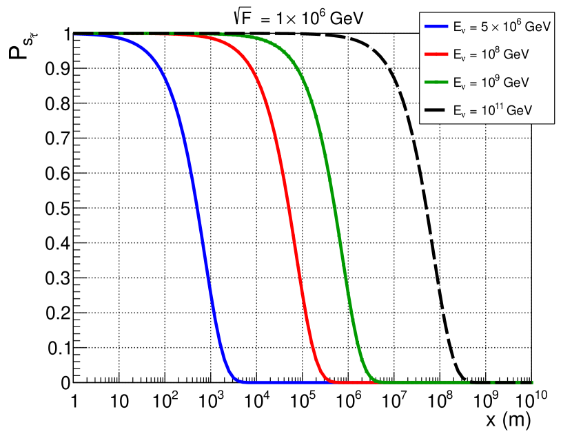
Figure 1: NLSP survival probability as a function of traveled distance, for different neutrino energies (as labeled) and $\sqrt{F}=10^{6}$ GeV.

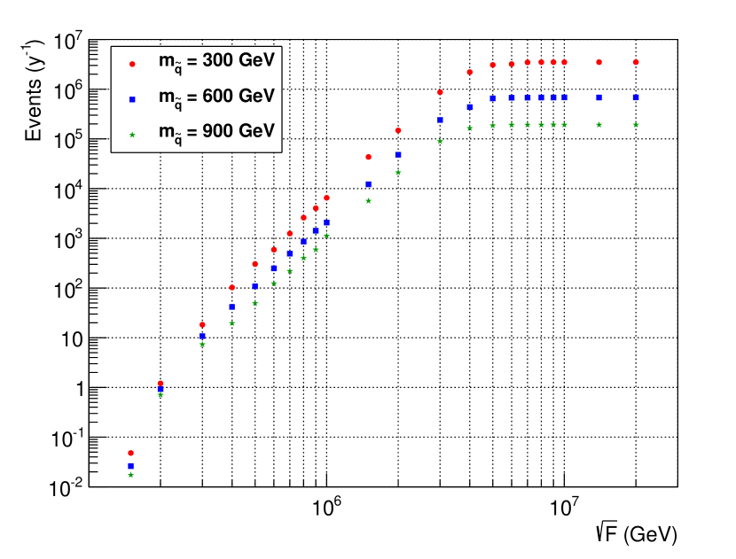
Figure 2: Fraction of NLSP events in JEM-EUSO’s field of view (FOV) versus $\sqrt{F}$ for $m_{\tilde{q}}$ reference values. NLSPs decay for $\sqrt{F}\begin{array}[]{c}\,\sim\vspace{-1.7em}\\ <\end{array}5\times 10^{6}$˜GeV.

We developed a Monte Carlo simulation, where $\vartheta(10^{5})$ events where generated, corresponding to neutrinos reaching the Earth, isotropically distributed both in energy and impinging direction. These events are normalized by the WB limit. The NLSP production, propagation and energy loss were simulated, reproducing the analysis shown in  abcd (see Section II).

The NLSP decay point is chosen from the decay probability distribution (essentially $1-P_{s}$), and the generated $\tau$ center of mass isotropic angular distribution is boosted into the laboratory frame. To a good approximation, it will follow the same direction as its parent NLSP. As two NLSPs are always generated in pairs, two $\tau$s will be produced. A fraction of these $\tau$s subsequently decay, always generating a $\nu_{\tau}$, which can charge current interact producing a new $\tau$. We determine the fraction of the $\tau$ energy carried by the $\nu_{\tau}$ as in crotty ; dutta . This regeneration process can happen a few times depending on the $\tau$ energy degradation. As mentioned before, this process will degrade the $\tau$ energy and most of them will not be detectable.

IV Signatures and Event Rates in the JEM-EUSO Observatory

In order to determine the feasibility of NLSP indirect detection, where $\tau$s originated in NLSP decays would be probed by a large fluorescence telescope, we have to consider basic detector features. The JEM-EUSO telescope euso will observe fluorescence light emitted from an extensive air shower created by the interaction of a high energy particle in the atmosphere. It will orbit the Earth at an altitude of about 430 Km, yielding a detection area of $\sim 2\times 10^{5}$ Km² with a 250 Km circular radius at the Earth surface. It is scheduled to be launched in 2016.

At these energies, NLSP produced $\tau$s can be observed by JEM-EUSO mainly through the shower created once they decay. NLSP direct detection is hard, since the energy of its emitted fluorescence light is much less than the detector threshold, which is projected to be around $10^{19}$ eV.

In order to determine the rate of observable events, we approximate the JEM-EUSO detection volume as a frustum of a cone, which represents the detector field of view. This is shown in figure 3. The frustum’s height corresponds to the atmosphere altitude which is taken as 40 Km.

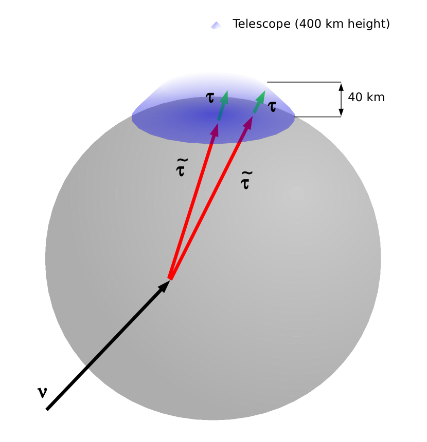
Figure 3: Representation of JEM-EUSO detection volume as a frustum of a cone, with a 40 Km height corresponding to the atmosphere altitude. NLSPs originated from neutrino interactions will decay in the atmosphere, producing observable $\tau$s.

As described in the previous section, we simulate NLSP production from neutrino interactions in the Earth, their propagation and energy loss and finally their decay. The neutrino energy ranges from $\sim 10^{6}$ to $\sim 10^{12}$ GeV, where the lower limit corresponds to the NLSP production threshold. As the NLSPs are always produced in pairs, two $\tau$s will be produced from their decay. Although the pair of NLSPs travel in parallel, they can decay at different times, and each $\tau$ can be produced at different positions. Each production point is independently chosen from the decay probability distribution.

The $\tau$ energy loss considers both ionization and radiation processes, where the latter includes loss due to bremsstrahlung, pair production and photo-nuclear interactions pdg ; abcd . We also follow the NLSPs which do not decay inside the Earth and reach the atmosphere, computing their energy and flux. The NLSP energy loss to the atmosphere is negligible.

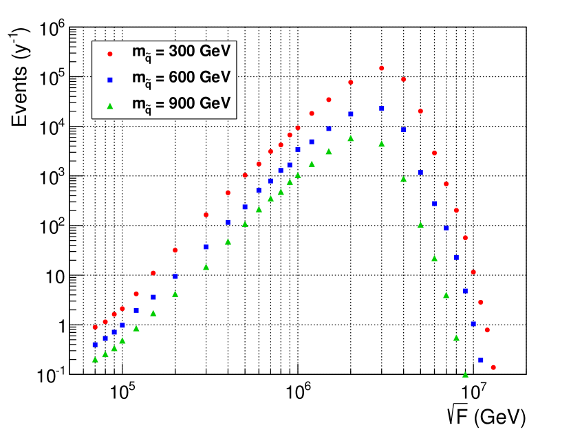
Figure 4: NLSP coincident decays in JEM-EUSO FOV as a function of $\sqrt{F}$.

In summary we compute the $\tau$ production point and initial energy distribution, as well as its decay point and energy distribution. These yield the number of $\tau$s which decay in or propagate through the detector field of view, and corresponding energy distributions. We also compute the number of coincident $\tau$ decays in the field of view. All results are normalized by the WB neutrino flux.

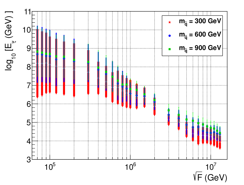
Figure 5: Average energy of events shown in Figure 4. Error bars represent standard deviation of each energy distribution.

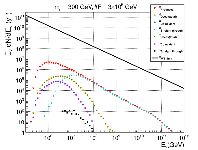
Figure 6: Events per year in JEM-EUSO FOV. Here $m_{\tilde{q}}=300$ GeV and $\sqrt{F}=3\times 10^{6}$ GeV, such that the number of events is maximized. The circles correspond to NLSPs (represented as $\tilde{\tau}$) and triangles to $\tau$s. The NLSP ($\tau$) that decay are in yellow (green), the ones that go through the FOV without decaying in light blue (black), the ones which both NLSPs produced as a pair (or both $\tau$s) decay in the FOV in blue (purple). As a reference the total number of NLSPs that are produced in the direction of the FOV are shown in red and the WB limit as a black line. Other values of $m_{\tilde{q}}$ will have similar curves but with less events.

Our results are presented as a function of $\sqrt{F}$. Figure 4 shows the number of coincident NLSP decays per year in JEM-EUSO field of view (FOV), while Figure 5 shows the NLSP average decay energy. As can be seen, the number of events is maximized for $\sqrt{F}=3\times 10^{6}$ GeV for both 300 and 600 GeV squark masses and $2\times 10^{6}$ GeV for $m_{\tilde{q}}=900$ GeV, due to its higher production energy threshold. However at these values of $\sqrt{F}$, the NLSP average decay energy is lower than the detection threshold, and increases for lower $\sqrt{F}$ values. We will further discuss this issue.

Figure 6 shows the number of events per year in JEM-EUSO FOV as a function of the parent neutrino energy, for $\sqrt{F}=5\times 10^{6}$ GeV which maximizes the number of events. It shows the NLSPs ($\tilde{\tau}$) and $\tau$s that decay, the ones that go through the FOV without decaying, the ones which both NLSPs produced as a pair or both $\tau$s decay coincidently in the FOV. As a reference, the figure also shows the total number of NLSPs that are produced in the direction of the FOV and the WB limit. This figure shows results assuming $m_{\tilde{q}}=300$ GeV, where for the other $m_{\tilde{q}}$ values the shape of the curves are very similar but contain less events. The total rate of events in JEM-EUSO per year, for our nominal value of maximum atmosphere height of 40 Km, for the three values of $m_{\tilde{q}}$, are shown in Table 1.

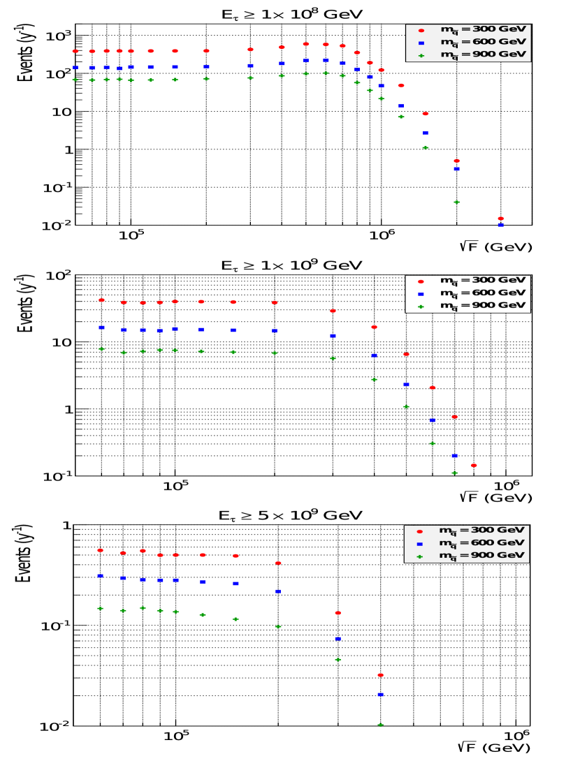
Figure 7: Total number of $\tau$ decays in JEM-EUSO FOV, requiring a minimal energy of $10^{8}$ GeV (top plot); $10^{9}$ GeV (middle plot) and $5\times 10^{9}$ GeV (bottom plot).

Table 1: Number of NLSP events per year in JEM-EUSO FOV, where $\sqrt{F}=3(2)\times 10^{6}$ GeV for $m_{\tilde{q}}=300,600(900)$ GeV. For $m_{\tilde{q}}=300$ GeV these events correspond to the ones shown in Figure 6. “Total” is the total number of NLSPs produced in the direction of the FOV; “Straight Through” refers to the NLSPs that go through the FOV; “Decay ” to those which decay in the FOV; and “Pair Decay” to the ones where the NLSP pair decays in coincidence in the atmosphere.”

$m_{\tilde{q}}$	Total	Straight Through	Decay	Pair decay
300	$1\times 10^{7}$	$8.7\times 10^{5}$	$5.2\times 10^{5}$	$1.5\times 10^{5}$
600	$1.3\times 10^{6}$	$2.4\times 10^{5}$	$9.6\times 10^{4}$	$2.2\times 10^{4}$
900	$2.8\times 10^{5}$	$2.0\times 10^{4}$	$1.9\times 10^{4}$	$5.8\times 10^{3}$

As seen in this table a huge amount of NLSPs should either go through or decay in JEM-EUSO FOV. As the NLSPs are not detectable due to the low amount of fluorescence emitted while they transverse the atmosphere, the hope of probing these events relies on the $\tau$s produced in their decay. However, although more than $10^{5}$ $\tau$s will tranverse or decay in JEM-EUSO FOV, most of these events have energies below the detector threshold ($\sim 10^{19}$ eV) and will not be observed unless this threshold is lowered.

In order to determine the event rate that can be observed with an energy threshold around the currently projected by JEM-EUSO, we selected events above arbitrary lower energy values of $10^{8},10^{9}$ and $5\times 10^{9}$  GeV. These are shown in Figure 7 and the integrated number of events, maximized as a function of $\sqrt{F}$, in Table 2.

Table 2: Number of $\tau$ events per year in JEM-EUSO FOV after requiring a minimum $\tau$ energy $E_{\tau}$. $\sqrt{F}$ is such that it maximizes the number of events. The line corresponding to $\sqrt{F}=3\times 10^{6}$ GeV is shown for reference and has no energy requirement.

$m_{\tilde{q}}$ = 300 GeV
$\sqrt{F}$ (GeV)	$E_{\tau}$ (GeV)	$\tau_{Decay(total)}$	$\tau_{Coincident}$
$3.0\times 10^{6}$		$5.5\times 10^{5}$	$1.5\times 10^{5}$
$6.0\times 10^{5}$	$\geq 10^{8}$	$5.8\times 10^{2}$	$1.0\times 10^{2}$
$1.5\times 10^{5}$	$\geq 10^{9}$	$3.9\times 10^{1}$	$4.2\times 10^{0}$
$1.2\times 10^{5}$	$\geq 5\times 10^{9}$	$5.0\times 10^{-1}$	$1.0\times 10^{-2}$
$m_{\tilde{q}}$ = 600 GeV
$3\times 10^{6}$		$9.8\times 10^{4}$	$2.2\times 10^{4}$
$6\times 10^{5}$	$\geq 10^{8}$	$2.2\times 10^{2}$	$3.8\times 10^{1}$
$1.2\times 10^{5}$	$\geq 10^{9}$	$1.5\times 10^{1}$	$1.6\times 10^{0}$
$2\times 10^{5}$	$\geq 5\times 10^{9}$	$2.0\times 10^{-1}$	$1.0\times 10^{-2}$
$m_{\tilde{q}}$ = 900 GeV
$2\times 10^{6}$		$2.0\times 10^{4}$	$5.8\times 10^{3}$
$6\times 10^{5}$	$\geq 10^{8}$	$1.0\times 10^{2}$	$1.8\times 10^{1}$
$1.2\times 10^{5}$	$\geq 10^{9}$	$7.2\times 10^{0}$	$8.0\times 10^{-1}$
$1.2\times 10^{5}$	$\geq 5\times 10^{9}$	$1.3\times 10^{-1}$	$6.0\times 10^{-3}$

As can be seen from Table 2 there is still a reasonable amount of events for a maximized $\sqrt{F}$ around JEM-EUSO energy threshold. Above $10^{18}$ eV, 39 (15, 7) $\tau$s can be detected per year, for a 300 (600, 900) GeV squark mass. From these 4 (2, 1) $\tau$ pairs decay in coincidence in the atmosphere, which provides an excellent discriminating signature. For a threshold of $5\times 10^{18}$ eV, a bit below the nominal projected threshold, 0.5 (0.2, 0.1) events per year can be observed by JEM-EUSO.

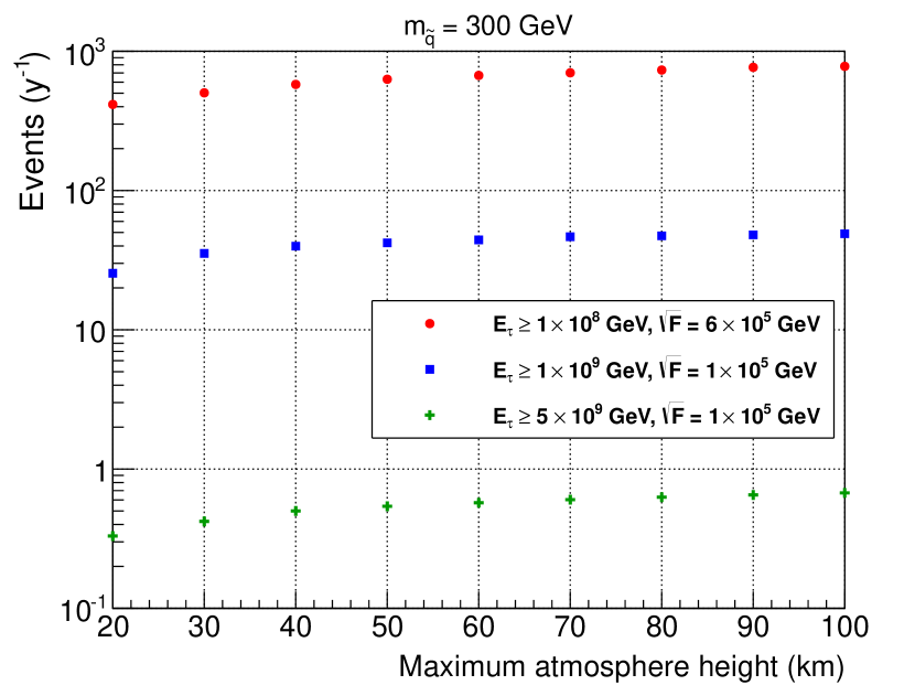
Figure 8: Number of $\tau$ decays as a function of the maximum atmosphere height, for different values of required minimal $\tau$ energy.

In Figure 8 we show the total number of $\tau$ decays as a function of the maximum atmosphere height, for different values of the required minimal $\tau$ energy. This allows one to rescale our results when considering different field of view heights. Although this figure is shown only for a $m_{\tilde{q}}=300$ GeV, the rescaling for other masses is about the same.

IV.1 Backgrounds

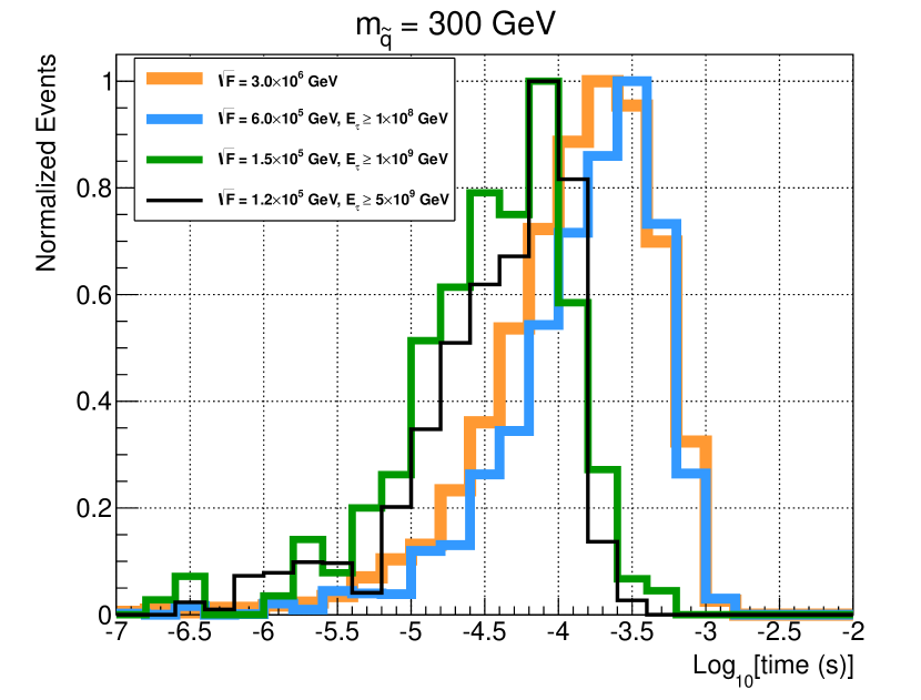
Figure 9: Time delay between two $\tau$ coincident decays in the atmosphere. Shown for arbitrary $\sqrt{F}$ and lower NLSP energy requirements. The squark mass is 300 GeV but it does not vary considerably for larger values.

Under the scenarios we are considering, NLSP decays will have a very distinctive signature. Since the NLSPs are produced inside the Earth and decay into $\tau$s that go upwards in the atmosphere, they can be discriminated from the more abundant down going cascades produced by normal ultra high energy cosmic rays.

Also a considerable fraction of the NLSP pairs decay in coincidence in the atmosphere. Figure 9 shows the distribution of the time delay between two $\tau$ decays in the atmosphere. These are shown for different $\sqrt{F}$ and energy lower limit requirements. It shows results for a 300 GeV squark mass, which do not vary significantly for larger values. The time delay spread as a function of $\sqrt{F}$ is small, and is distributed around $10^{-4}$ s. Considering that an atmospheric shower takes about 0.3 seconds, and that the detector resolution is about 2.5 $\mu$s, it is possible to determine the coincidence of these decays.

Figure 10 shows the distance between the coincidence showers, considering the same parameters as for the previous figure. Given that the detector spacial resolution is about 0.75 Km, it is clear that the majority of the coincident showers can be well distinguished.

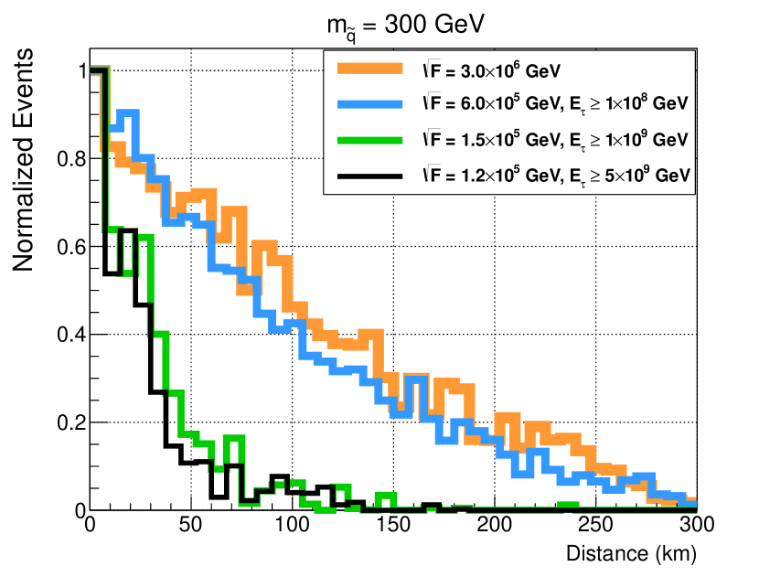
Figure 10: Distance between two $\tau$ decays in the atmosphere, assuming same parameters as in the previous figure.

V Discussion And Conclusions

In order to understand the effect of the experimental energy threshold, we showed our results for arbitrary lower energy cuts. As shown in Table 2 , the lower threshold has a significant effect on how well large fluorescence telescopes can probe the supersymmetry breaking scale.

While an experimental energy threshold of $10^{18}$ eV allows JEM-EUSO to discover NLSP produced $\tau$s and consequently probe a significant $\sqrt{F}$ region, a $10^{19}$ eV allows to set limits in the production and $\sqrt{F}$ parameters. Table 2 shows that, for a maximum value of $\sqrt{F}$, $\vartheta(10^{5})$ of detectable events will go through JEM-EUSO FOV. From these hundreds of events per year can be seen if the energy threshold is set to $10^{17}$ eV, while tens for $10^{18}$ and more than a year is needed to detect events for $10^{19}$ eV. Although these numbers are for a maximized value of $\sqrt{F}$, one can see from Figure 7 that there is a significant range, in which $10^{5}\begin{array}[]{c}\,\sim\vspace{-1.7em}\\ <\end{array}\sqrt{F}\begin{array}[]{c}\,\sim\vspace{-1.7em}\\ <\end{array}10^{6}$ GeV, that can be probed with the same order of events.

We have shown that large fluorescence telescopes such as JEM-EUSO have the potential to indirectly detect NLSPs which are modeled in various supersymmetry breaking scenarios. We show that scenarios where the supersymmetry breaking scale $\sqrt{F}$ is such that the NLSP will decay close to or in the atmosphere can be probed by JEM-EUSO. Depending on the experimental energy threshold, scenarios with $10^{5}\begin{array}[]{c}\,\sim\vspace{-1.7em}\\ <\end{array}\sqrt{F}\begin{array}[]{c}\,\sim\vspace{-1.7em}\\ <\end{array}10^{6}$ can be probed, and NLSPs can be indirectly searched.

This work complements the direct probe for long-lived NLSPs abc ; abcd , where scenarios with $5\times 10^{6}\begin{array}[]{c}\,\sim\vspace{-1.7em}\\ <\end{array}\sqrt{F}\begin{array}[]{c}\,\sim\vspace{-1.7em}\\ <\end{array}5\times 10^{8}$ can be directly probed by neutrino telescopes. It is also complementary to searches for NLSP decays at the LHC.

- (1) I. Albuquerque, G. Burdman and Z. Chacko, Phys. Rev. Lett. 92, 221802 (2004) [arXiv:hep-ph/0312197] .
- (2) I. Albuquerque, G. Burdman and Z. Chacko, Phys. Rev. D 75, 035006 (2007) [arXiv:hep-ph/0605120].
- (3) I. F. M. Albuquerque, G. Burdman, C. A. Krenke and B. Nosratpour, Phys. Rev. D 78, 015010 (2008) [arXiv:0803.3479 [hep-ph]].
- (4) G. F. Giudice and R. Rattazzi, Phys. Rept. 322, 419 (1999) [hep-ph/9801271].
- (5) Jairo Cavalcante de Souza, PhD. Thesis, http://www.teses.usp.br/teses/disponiveis/, Universidade de São Paulo, in portuguese, São Paulo (2012).
- (6) I. F. M. Albuquerque and J.Cavalcante de Souza. arXiv:1210.5141 [hep-ph] (2012).
- (7) F. Kajino et al. [JEM-EUSO Collaboration], AIP Conf. Proc. 1367, 197 (2011); http:jemeuso.riken.jp/en/index.html
- (8) E. Waxman and J. N. Bahcall, Phys. Rev. D 59, 023002 (1999); J. N. Bahcall and E. Waxman, Phys. Rev. D 64, 023002 (2001).
- (9) J. Beringer et al. (Particle Data Group), Phys. Rev. D86, 010001 (2012).
- (10) M. Kawasaki, K. Kohri, T. Moroi and A. Yotsuyanagi, Phys. Rev. D 78, 065011 (2008) [arXiv:0804.3745 [hep-ph]].
- (11) Adam Dziewonski, Earth Structure, Global, in The Encyclopedia of Solid Earth Geophysics, edited by David E. James (Van Nostrand Reinhold, New York, p. 331 (1989).
- (12) R. Gandhi, C. Quigg, M. H. Reno and I. Sarcevic, Astropart. Phys. 5, 81 (1996); R. Gandhi, C. Quigg, M. H. Reno and I. Sarcevic, Phys. Rev. D 58, 093009 (1998).
- (13) M. H. Reno, I. Sarcevic and S. Su, Astropart. Phys. 24, 107 (2005) [arXiv:hep-ph/0503030].
- (14) P. R. Crotty, FERMILAB-THESIS-2002-54 (2002).
- (15) S. I. Dutta, M. H. Reno and I. Sarcevic, Phys. Rev. D 62, 123001 (2000) [hep-ph/0005310].