Deep blank field catalogue for medium- and large-size telescopes

Abstract

The observation of blank fields, defined as regions of the sky that are devoid of stars down to a given threshold magnitude, constitutes one of the most relevant calibration procedures required for the proper reduction of astronomical data obtained following typical observing strategies. In this work, we have used the Delaunay triangulation to search for deep blank fields throughout the whole sky, with a minimum size of 10′ in diameter and an increasing threshold magnitude from 15 to 18 in the R band of the USNO-B Catalog of the United States Naval Observatory. The result is a catalogue with the deepest blank fields known so far. A short sample of these regions has been tested with the 10.4m Gran Telescopio Canarias, and it has been shown to be extremely useful for medium and large size telescopes. Because some of the regions found could also be suitable for new extragalactic studies, we have estimated the galactic extinction in the direction of each deep blank field. This catalogue is accessible through the Virtual Observatory tool TESELA, and the user can retrieve - and visualize using Aladin - the deep blank fields available near a given position in the sky.

1 Introduction

In observational astrophysics, and in particular focusing in imaging acquisition through the optical window, the data treatment is fundamental to minimize the influence of data acquisition imperfections on the estimation of the desired astronomical measurements (e.g. Gilliland 1992). For this purpose, image flat-fielding and sky subtraction constitute two of the most common and important reduction steps. An inadequate flat-fielding or sky subtraction easily leads to the introduction of systematic uncertainties in the data. Therefore, the observation of blank fields (BFs), defined as regions of the sky that are devoid of stars down to a given threshold magnitude ($m_{\mbox{\scriptsize th}}$), is a very important aspect in astronomical observations. In our previous paper Cardiel et al. (2011) (hereafter Paper I), we have already discussed in detail the relevance of BFs in astronomical observations, and we refer the interested reader to the introduction of that paper.

In Paper I, we presented the first systematic all-sky catalogue of BFs so far. The method used to identify the BFs was based on the Delaunay triangulation on the surface of a sphere, using stars brighter than 11 mag taken from the Tycho-2 (Høg et al., 2000) catalogue as the nodes for triangulation. In addition, a new Virtual Observatory (VO) tool named TESELA, accessible through the internet, was created so that users can retrieve, and visualize, the BFs available near a given position in the sky.

Another commonly used resource is the collection by Marco Azzaro, consisting of a short list of 38 BFs voids of stars up to 10–16 mag. Although, in general, deeper than the BFs of Paper I, these are very few, and most of them are in the Northern hemisphere; there are only a few with negative declination, and none bellow $-20^{\circ}$. So, this BF collection is not well suited for telescopes located in the Southern hemisphere.

Nevertheless, even the Azzaro BFs have been shown to be shallow for large-class telescopes. For example, in the case of the Gran Telescopio Canarias (GTC), a 10-m class telescope, equipped with the Optical System for Imaging and Low Resolution Integrated Spectroscopy (OSIRIS, Cepa et al., 2000), it is usually necessary to have access to BFs free of stars down to 17.5 mag. This requirement will be even more demanding for the future generation of telescopes, such as European Extremely Large Telescope (E-ELT).

One method of identifying low-populated fields is to use a binned-up smoothed map of the distribution of the stars in the sky. In this method, it is necessary to divide the sky in small patches and to identify those with few, or even no stars, down to a threshold magnitude. However, with this method, a BF would not be identified unless the patch was well centered on the region free of stars. In addition, the size of the BF would not be the maximum possible because it is arbitrarily defined. Thus, the procedure should be repeated many times with both a different centring scheme and a different patch radius; this would be very demanding with respect to CPU time. These two drawbacks can be overcome with the sky tessellation method we have developed, which has been extensively described in Paper I.

Thus, in this work we have applied Delaunay triangulation to the USNO-B Catalog of the United States Naval Observatory, we have generated acatalogue of deep blank fields (DBFs) to varying limiting magnitudes from 15 to 18 in steps of 1 mag. In order to validate our method, we have tested some DBFs found at the GTC and we have compared these with the BFs in Azzaro catalogue. Finally, in order to facilitate the use of this new catalogue, we have incorporated it into TESELA, which now provides a simple interface that allows the user to retrieve the list of either the BFs from Tycho-2 or the DBFs from USNO-Bavailable near a given position in the sky.

In Section 2, we describe the method used to create the catalogues, the defects found in the USNO-B Catalog and the results of the tessellation. Section 3, we describe the use of the DBFs catalogue on the GTC. And, finally, in Section 4, we describe the implementation of TESELA.

2 The catalogue

2.1 Tessellating the sky

The Delaunay triangulation (Delaunay, 1934) consists of the subdivision of a geometric object (e.g. a surface or a volume) into a set of simplices. In particular, for the Euclidean planar (two-dimensional) case, given a set of points, also called nodes, Delaunay triangulation becomes a subdivision of the plane into triangles, whose vertexes are nodes. For each of these triangles, it is possible to determine its associated circumcircle, which is the circle passing exactly through the three vertices of the triangle. Interestingly, in a Delaunay triangulation, all the triangles satisfy the empty circumcircle interior property, which means that all the circumcircles are empty (i.e. there are no nodes inside any of the computed circumcircles). See Paper I for an extended description of the method.

Delaunay triangulation can be applied to the two-dimensional surface of a three-dimensional celestial sphere, using as nodes the locations of the stars down to a given $m_{\mbox{\scriptsize th}}$. Then, the empty circumcircle interior property of the Delaunay triangulation provides a straightforward method for a systematic search of regions void of stars brighter than a certain magnitude.

In this work we applied the Delaunay triangulation to the sources of the USNO-B Catalog (Monet et al., 2003). The USNO-B Catalog contains astrometric and photometric information for more than a billion stars and galaxies in the sky. The data were taken from various sky surveys over 50 years, and it is expected to be complete up to magnitude V = 21 mag. Typical uncertainties are 200 mas for the positions at J2000 and 0.3 mag in photometry. Photometric data consists of V, R, and I optical passbands. We used the R band (between 600 and 750 nm) as the magnitude reference. For most of the sources, the USNO-B Catalog provides the R magnitude ($m_{\mbox{\scriptsize R}}$) at two different epochs. To assign a single $m_{\mbox{\scriptsize R}}$ to these objects, either we have averaged out both $m_{\mbox{\scriptsize R}}$ when their values are similar ($\Delta m_{\mbox{\scriptsize R}}$ $<$1) or selected the lower value (i.e., the brightest value) when there is a larger difference.

In principle, it is straightforward to obtain a list of BFs for the whole celestial sphere by using as input a stellar catalogue including stars down to a given magnitude. However, as explained in Paper I, because of the exponential growth of the number of objects with increasing limiting magnitude, tessellating the whole sky with $m_{\mbox{\scriptsize th}}$ above 11 mag requires too many computer resources (in form of memory and computing time), even with the approach of subdividing the sky into many smaller subregions.

Therefore, to create the DBFs catalogue, we have followed a methodology that is different from the one adopted in Paper I. Instead of tessellating the whole sky at once, we used the following workflow. (i) We selected all BFs with a size larger than 10′, using the deepest catalogue available at that moment. (ii) We individually tessellated each of these regions, as in Paper I, using the positions of the USNO-B objects down to a $m_{\mbox{\scriptsize th}}$ as the nodes of the triangulation. (iii) To create the new DBFs catalogue, from the new collection of deeper BFs we selected those with a size larger than 10′. (iv) We repeated the whole process, increasing $m_{\mbox{\scriptsize th}}$ from 15 to 18 in steps of 1 mag.

The initial collection of BFs was obtained from Paper I, consisting of BFs void of stars down to 11 mag in both Tycho-2 passbands. This provided $1\,477\,348$ initial regions with a size larger than 10′. This size was selected to ensure that the regions were always larger than the field of view of the OSIRIS instrument used at the GTC (see Sect.3). Tessellating this huge number of initial regions requires months of execution time. In order to obtain the results as soon as possible so they could be used in the nightly operation of the GTC, we proceeded with the Northern (Dec $>$ $-$30^∘) sky in strips 1 h wide in RA. When the tessellation of the Northern sky was finished, we tessellated the Southern (Dec $\leq$ $-$30^∘) sky in the same way. Finally we merged all DBFs found in one catalogue.

It was very common that the tessellation process identified two overlaping DBFs which centers were separated by less than 0.3 times the smaller DBF radius. Although both DBFs are correct, the two refer to almost the same region of the sky. Thus, to facilitate the use of the catalogue, we removed the DBF with the smaller radius from the catalogue, retaining the one with the larger size.

A final evaluation of each DBF of the catalogue was made. We counted the total number of stars inside the DBF with both $m_{\mbox{\scriptsize R}}$ lower than 17.5 mag (a requirement of the GTC; see Section 3) and lower than 22.0 mag. Then, we estimated the integrated R flux ($F_{\mbox{\scriptsize int}}$) as the sum of the individual fluxes of all star in the DBF with $m_{\mbox{\scriptsize R}}$ $<$ 22.0 mag. These quantities provided a measurement of the depth of the DBF.

To verify the validity of the method, and taking advantage of the Aladin software Bonnarel et al. (2000), we visually checked all the 79 DBFs of 18 $m_{\mbox{\scriptsize th}}$ found previously in order to give them to the operation staff of the GTC. This VO tool allows users to visualize and analyse digitized astronomical images, and superimpose entries from astronomical catalogues or data bases available from the VO services. Using Aladin, we displayed the DSS-red images of the DBF region and we superimposed the USNO-B data of the region. This exercise was very useful in the detection of unknown defects in the USNO-B Catalog (see Sect.2.2). Of the 79 DBFs, 5 corresponded to a dark cloud, so they were removed from the final catalogue. Similarly, we removed any DBFs corresponding to the same dark cloud of any $m_{\mbox{\scriptsize th}}$.

2.2 Defects in the USNO-B Catalogue

The USNO-B Catalog was constructed from photographic plates, taken from several different surveys, which were uniformly scanned, and whose sources were extracted in an automatic way from the scanned data. The original plate images contained many defects and artifacts that logically affected the final USNO-B data. That said, so far there is no other full sky catalogue deep enough for our project. So, the USNO-B Catalog was our best option, even with its known defects. Because we have used the USNO-B Catalog as the input for the tesellation process, our DBF catalogue was affected by the defects of the USNO-B Catalog. Although we have made an effort to minimise the damage, we cannot completely guarantee the absence of misidentification in our final DBF catalogue. So, the user should confirm the validity of the DBFs before using them.

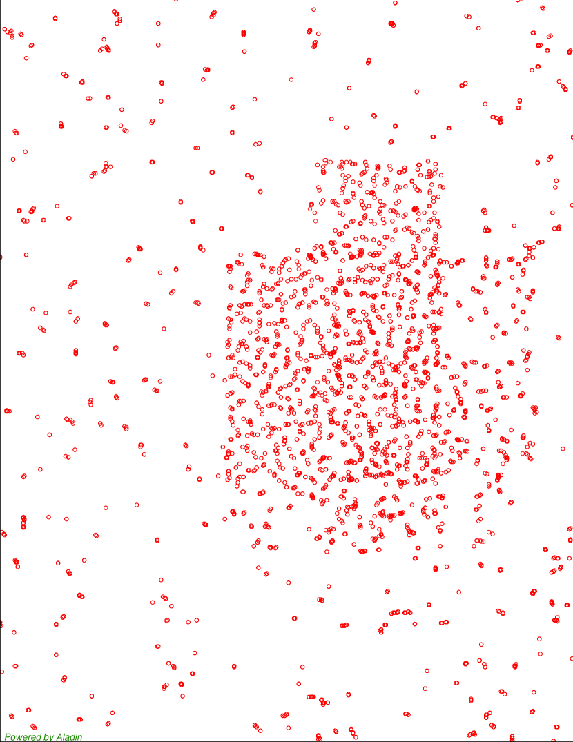
Figure 1: Abnormal concentration of DBFs with $m_{\mbox{\scriptsize th}}$ = 15 in the region of the sky of 12^∘$\times$12^∘centered at ($\alpha_{J2000}$,$\delta_{J2000}$) = (30^∘,00^∘).

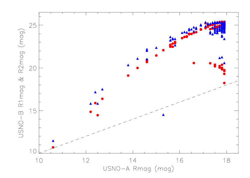
Figure 2: Comparison between USNO-A Rmag and USNO-B R1mag (red circles) and R2mag (blue triangles) magnitudes of the common objects in region of the sky centered at ($\alpha_{J2000}$,$\delta_{J2000}$) = (31.9^∘,–37.1^∘) and with a radius if 8.5′. Dashed line depicts the one-to-one correlation.

During the first inspection of the sky distribution of the DBFs found, we realized that there were abnormal concentrations of DBFs in two rectangular-shaped regions, one around ($\alpha_{J2000}$,$\delta_{J2000}$) = (30^∘,00^∘) and the other around (27^∘,–37^∘); see Fig. 1. This high density of DBFs reflects an abnormally high value of the $m_{\mbox{\scriptsize R}}$ in the USNO-B Catalog, probably because of a wrong photometric calibration of the photographic plates. In Fig. 2 we show a comparison between USNO-A Rmag and USNO-B R1mag and R2mag of the objects in common in a small region of the sky where abnormally high density of DBFs was found. The values of USNO-B R1mag and R2mag are usually more than 7 mag higher than those of USNO-A Rmag. Thus, the DBFs found on this region were clearly unreliable. Then, we defined four rectangular regions (see Table 1) covering the areas with an abnormally high density of DBFs and used the USNO-A Catalog in the tessellation instead of USNO-B Catalog.

Table 1: Regions where USNO-A Catalog was used instead of USNO-BCatalog.

RA (∘)		DEC (∘)
(J2000)
min	max	min	max
21.75	32.70	–37.86	–32.91
23.25	28.95	–42.46	–37.75
28.95	31.20	+2.01	+3.56
27.64	32.45	–2.65	+2.09

Barron et al. (2008) have found that $\sim$2.3 per cent of the USNO-B Catalog entries do not correspond to real astronomical sources; they are mainly - but not only - spurious entries, caused by diffraction spikes and circular reflection haloes around bright stars in the original imaging data (see figs 1, and 2 of their paper). In our search for DBFS, the effect of these spurious entries is clear; some of the DBFs might not have been found during the process because of the presence of one or more spurious sources in the field. Thus, these spurious entries might have decreased the number of DBFs, but they have never introduced unreal DBF detections.

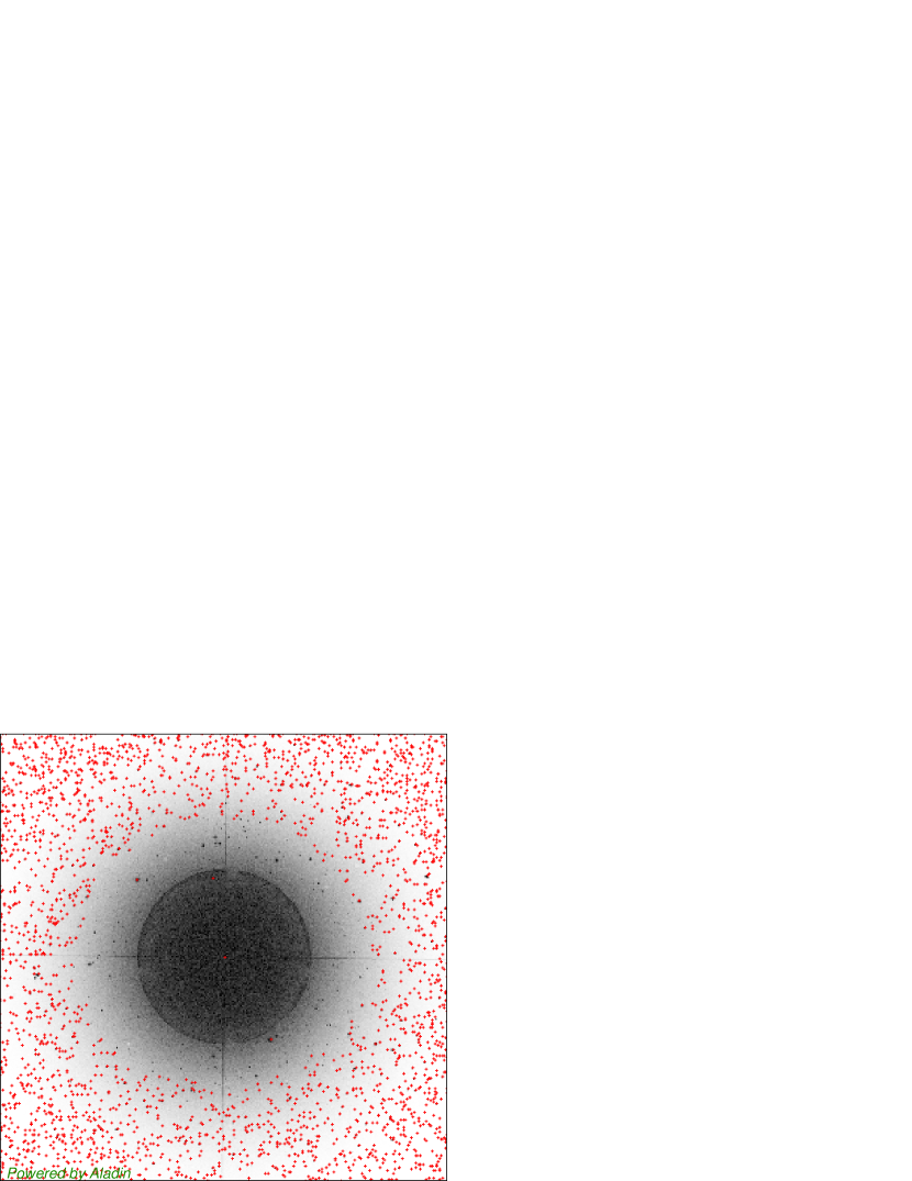
Figure 3: USNO-B Catalog entries superimposed to the DSS-red 30′$\times$30′ image centered at Vega.

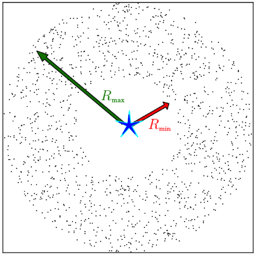
Figure 4: Illustration of the parameters defined for the automatic determination of the radii around bright stars, which are devoid of neighbouring (fainter) stars. The parameter sought is $R_{\mbox{\scriptsize min}}$, where $R_{\mbox{\scriptsize max}}$ is the maximum region around the bright object where star density is determined. The basic hypothesis of the method is the assumption that the stellar density in the annulus between $R_{\mbox{\scriptsize min}}$ and $R_{\mbox{\scriptsize max}}$ is roughly constant.

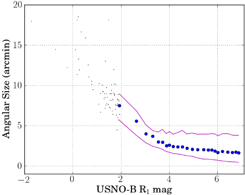
Figure 5: Variation of the size of the artificial void-of-stars regions with the USNO-B R1mag. For stars brighter than $m_{\mbox{\scriptsize R}}=2$ mag (small black dots), the radius devoid of neighbouring stars is shown for each individual star. For stars fainter that $m_{\mbox{\scriptsize R}}=2$ mag, the median of the radii are plotted as blue filled circles. The magenta lines indicate the percentiles 15.9 and 84.1 (which approximately correspond to $\pm 1\sigma$ confidence limits in a normal distribution).

However, there are other defects in the USNO-B Catalog that could affect our tessellation process in a worse way. In Fig. 3, we show the USNO-B Catalog entries around Vega, which is one of the brightest stars of our sky. The brightest stars ($<$7 mag) are surrounded by a circular halo in the plate images, caused by internal reflections in the camera. Consequently, the regions around the brightest stars in the USNO-B Catalog are artificial regions that are void-of-stars, and in many cases these have been wrongly identified as DBFs.

With the help of the scripting capabilities of Aladin, we have estimated the radius of the region devoid of neighbour stars around each of the $25\,406$ USNO-B stars down to $m_{\mbox{\scriptsize R}}=7.0$ mag. For that purpose (see Fig. 4), we consider that around the bright stars there is a region devoid of stars up to a radius $R_{\mbox{\scriptsize min}}$. The automatic determination of this parameter is not difficult if we assume that the stellar density beyond this radius, and up to $R_{\mbox{\scriptsize max}}$ (which, in our case was set to 30′), is constant. Under this circumstance, it is easy to show that the number of stars within a radius $r$ (with $r>R_{\mbox{\scriptsize min}}$) is given by

$$N(<r)=N_{\mbox{\scriptsize tot}}\;\frac{r^{2}-R_{\mbox{\scriptsize min}}^{2}}{R_{\mbox{\scriptsize max}}^{2}-R_{\mbox{\scriptsize min}}^{2}},$$ (1)

where $N_{\mbox{\scriptsize tot}}$ is the total number of neighbouring stars in the annulus between $R_{\mbox{\scriptsize min}}$ and $R_{\mbox{\scriptsize max}}$. Because we were interested in obtaining an automatic and robust estimation of $R_{\mbox{\scriptsize min}}$, we have followed an approach based on the incomplete method of Thail (see e.g. De Muth 2006). As with most non-parametric procedures, all the objects in the field (within $R_{\mbox{\scriptsize max}}$) were first sorted in ascending order using the distance from the central bright star. This provided a collection of $N_{\mbox{\scriptsize tot}}$ points of coordinates $(R_{i},N_{i})$ where $i=1,2,3,....,N_{\mbox{\scriptsize tot}}$. Here, $R_{i}$ is the distance from the centre and $N_{i}$ is the number of objects within the circle of radius $R_{i}$. From any pair of such points, and considering equation (1), it is possible to obtain an estimation of $R_{\mbox{\scriptsize min}}$ as

$$R_{\mbox{\scriptsize min}}^{2}=\frac{N_{b}\;R_{a}^{2}-N_{a}\;R_{b}^{2}}{N_{b}-N_{a}},$$ (2)

where $R_{\mbox{\scriptsize min}}\leq R_{a}<R_{b}\leq R_{\mbox{\scriptsize max}}$. In this way, it is possible to compute $N_{\mbox{\scriptsize tot}}/2$ values for $R_{\mbox{\scriptsize min}}$ by using the last equation on pairs of points where $a=1,2,3,...,N_{\mbox{\scriptsize tot}}/2$ and $b=a+N_{\mbox{\scriptsize tot}}/2$ (in fact, this is the basics of the Thail method). Finally, we have determined the median of the $N_{\mbox{\scriptsize tot}}/2$ estimates of $R_{\mbox{\scriptsize min}}$.

In Fig. 5, we show the variation of the size of the region devoid of neighbouring stars, computed inthe way just explained, with $m_{\mbox{\scriptsize R}}$. On the basis of this diagram, we applied the following conservative criterion to avoid false DBFs in our catalogue: we have removed all DBFs whose centres were closer than 25′to stars with $m_{\mbox{\scriptsize R}}$ $\leq$ 0.5, 15′to stars with 0.5 $<$ $m_{\mbox{\scriptsize R}}$ $\leq$ 3.0, and 10′to stars with 0.3 $<$ $m_{\mbox{\scriptsize R}}$ $\leq$ 6.0. This criterion was not applied to the DBF with 18 $m_{\mbox{\scriptsize th}}$, because they were all visually inspected. The percentages of removed DBFs are 1, 2, and 9% for 15, 16, and 17 $m_{\mbox{\scriptsize th}}$, respectively. As expected, the percentage increases with $m_{\mbox{\scriptsize th}}$ because the number of wrong DBFs should be similar for all catalogues.

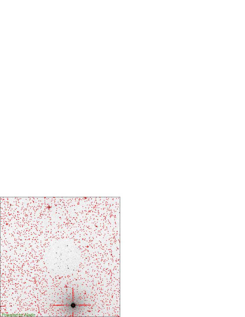
Figure 6: USNO-B Catalog entries superimposed to the DSS-blue 30′$\times$30′image centered at ($\alpha_{J2000}$,$\delta_{J2000}$) = (111.689^∘,$-$78.893^∘).

In Fig. 6, we show another defect of the USNO-B Catalog. There are no entries in a circular region of $\sim$9′diameter around the position in the sky ($\alpha_{J2000}$,$\delta_{J2000}$) = (07:26:40,$-$78:53:50). Our tessellation process detected this region as void of star and it has included a corresponding BF entry in the catalogue. The same problem occurred with another region of $\sim$16′diameter around ($\alpha_{J2000}$,$\delta_{J2000}$) = (20:12:40,$-$74:14:39). These two false void-of-star regions were detected by a change in the visual inspection of the DBFs, so we cannot discard further similar defects in the USNO-B Catalog, and consequently the possible presence of spurious BFs in our catalogue. These two detected spurious entries were manually rejected from our catalogue.

2.3 Results

The final result is a catalogue that is currently the deepest catalogue of regions that are void of stars. The catalogue is accessible through the TESELA tool (as explained in Section 4).

Table 2 presents the quantitative description of the above results. Column 1 gaves the threshold magnitude $m_{\mbox{\scriptsize th}}$ and column 2 lists the number of DBF regions found $N_{\mbox{\scriptsize DBF}}$. Columns 3, 4, and 5 indicate the mean radius $\overline{\rho}$, the standard deviation $\sigma_{\rho}$, and the maximum DBF radius $\rho_{\mbox{\scriptsize max}}$, respectively. The integrated mean flux $\overline{F_{{\mbox{\scriptsize int}}}}$, the standard deviation $\sigma_{F_{\mbox{\scriptsize int}}}$, and the minimum integrated flux $F_{\mbox{\scriptsize min}}$ and maximum integrated flux $F_{\mbox{\scriptsize min}}$ are given in columns 6, 7, 8, and 9, respectively.

Table 2: Results of the tessellation process using the USNO-B Catalog with the R filter.

(1)	(2)	(3)	(4)	(5)	(6)	(7)	(8)	(9)
$m_{\mbox{\scriptsize th}}$	$N_{\mbox{\scriptsize DBF}}$	$\overline{\rho}$	$\sigma_{\rho}$	$\rho_{\mbox{\scriptsize max}}$	$\overline{F_{{\mbox{\scriptsize int}}}}$	$\sigma_{F_{\mbox{\scriptsize int}}}$	$F_{\mbox{\scriptsize min}}$	$F_{\mbox{\scriptsize max}}$
(mag)		(′)	(′)	(′)	(erg/s/cm2/A)	(erg/s/cm2/A)	(erg/s/cm2/A)	(erg/s/cm2/A)
a11.0	1.477.348	10	4	51.2
15.0	77.277	5.5	0.5	14.2	1.6e-14	7.0e-15	2.3e-17	2.2e-13
16.0	6.062	5.4	0.5	12.8	8.5e-15	3.0e-15	3.1e-16	3.2e-14
17.0	332	5.6	0.7	9.0	3.8e-15	1.9e-15	1.5e-16	1.2e-14
18.0	74	5.8	0.8	9.0	1.8e-15	9.3e-16	3.1e-16	4.8e-15

• From the 11 threshold magnitude catalogue of Paper I obtained with the combination of Tycho-2 B and V bands.

In Fig. 7, we show the maps of the DBFs found in galactic coordinates (IAU 1958). As expected, the major concentration of DBFs is close to the galactic poles, with a low number of DBFs close to the galactic plane.

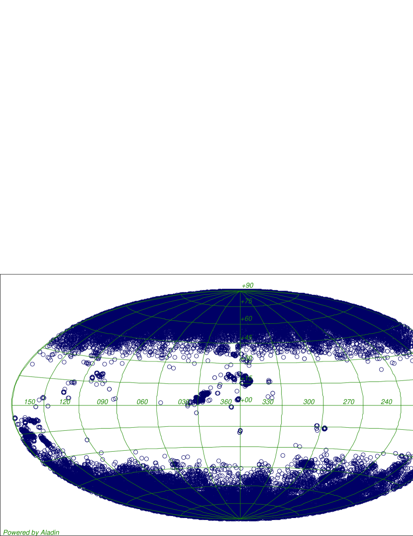
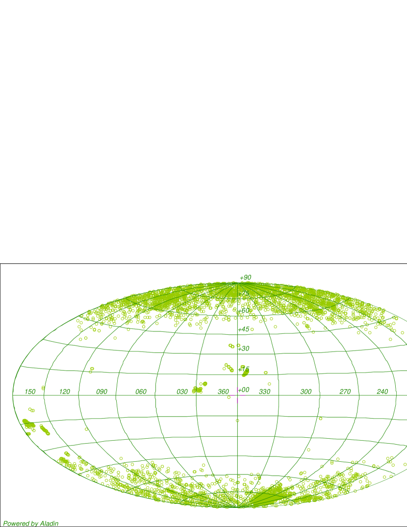
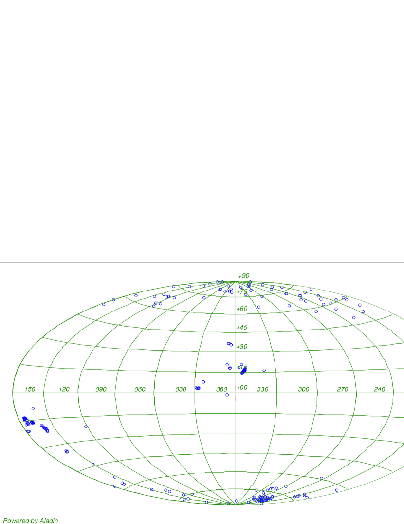
Figure 7: Galactic positions of the DBFs with $m_{\mbox{\scriptsize th}}$ 15, 16, 17, and 18 in the upper-left, upper-right, lower-left, and lower-right panel, respectively.

In order to provide a short list of DBFs that can be used at the telescope, we have selected, among the best regions found, one DBF for approximately a half hour in RA in each hemisphere, as provided in the Table LABEL:northDBFs. The equatorial and galactic coordinates are given first (columns 1–4). The radius $\rho$ of the DBF is given in column 5. The number of stars $N_{*}$ with $m_{\mbox{\scriptsize R}}$ lower than 17.5 and 22.0 mag are listed in columns 6 and 7, respectively. Columns 8 and 9 show $m_{\mbox{\scriptsize R}}$ of the faintest and brightest star in the field. The integrated flux $F_{{\mbox{\scriptsize int}}}$ is in column 10. The last four columns 11–14 give the galactic extincition $E(B-V)$ as described below. There are some regions at the Southern hemisphere where no DBFs have been found. Some of these DBFs have been validated with the GTC and are they are regularly used in the nightly operation of the telescope (see Section 3).

Although our main goal in this work was to provide a list of DBFs for data calibration, the DBFs found can also be used for other interesting purposes (e.g. deep pencil-beam extragalactic surveys). In this sense, the galactic extinction in the direction of the sky where the DBFs are located is useful information that would help in the identification of suitable DBFs. Thus, we used The Galactic Dust Reddening and Extinction utility of the NASA/ IPAC Infrared Science Archive to estimate the galactic extinction from Schlegel, Finkbeiner, & Davis (1998) for each DBF in our catalogue. In this way, five new parameters were added to the catalogue: $E(B-V)$ at the center of the DBF, the average $E(B-V)$ in the sky region defined by the DBF, together with its standard deviation, and the maximum and minimum $E(B-V)$ in this sky area.

3 Deep blank fields for OSIRIS/GTC

We have used the 10.4m GTC, located at Observatorio Roque de los Muchachos in La Palma (ORM), Canary Islands, Spain, as a test-bed for the validation of our DBFs. The telescope is currently equipped for scientific exploitation with the OSIRIS optical facility, which includes imaging with broad-band filters from the Sloan set ($ugriz$), as well as a very flexible set of narrow-band filters that can be used when requested.

The OSIRIS instrument consists of a mosaic of two Marconi CCD detectors, each with 2048 $\times$ 4096 pixels and a total unviggnetted field of view of 7.8 $\times$ 7.8′, giving a plate scale of 0.127″/pix. For this reason, the series of BFs requested for the nightly operation of the instrument must be at least 10′wide, it must be larger than the OSIRIS field of view, and it must also take into account the dithering between consecutive exposures that is usually performed to eliminate the contribution of the stars in producing the final flat-field image.

To date, the most comprehensive list of BFs available for observations carried out at the ORM has been the collection made by Azzaro. However, the large aperture of the GTC means that these fields (which are empty up to magnitudes 10–16) are too shallow to be used as BFs for the GTC, because they appear relatively full of stars once an OSIRIS/GTC image is obtained.

During the nightly operation of OSIRIS/GTC, an automatic script is used to obtain a series of broad-band flat-field images in Sloan $griz$ filters (Sloan $u$ filter is of rare use). Because of the particularities of the OSIRIS shutter, in order to obtain a photometric accuracy better than 0.1% in the images, exposure times of the order of 1–2 s are needed. To define the limiting magnitude for the BFs to be used at the GTC, a complete set of Azzaro fields was observed over nearly a year of operation at the telescope, and were reduced photometrically to determine the magnitude of the detected stars under good photometric conditions. For 1–2 s of exposure time, in Sloan $r$ filter, and with nearly 30 000 ADUs of sky background level (which represents half of the full well of the detector), stars as faint as 17.5–18.0 mag (depending on the seeing conditions) were detected. This is the fainter limit that we have imposed on the BFs to be used with OSIRIS/GTC, which might be empty regions of the sky up to $r^{\prime}=17.5$ mag. This is impossible to achieve with the Azzaro catalogue. In addition, for operating reasons, those BFs should provide a complete RA coverage. These two constraints are very restrictive, but they can sometimes be met using our DBF catalogue. Thus, we have been able to create a list of 87 DBFs that can be used with OSIRIS/GTC, although it was not always possible to archive the $m_{\mbox{\scriptsize th}}$ limit. This list provides at least one of these DBFs both at the beginning or at the end of every night of the year, which is extremely useful for the calibration of the scientific data delivered by OSIRIS instrument. This list has superseded the Azzaro catalogue in the nightly operation of the telescope. Some of the DBFs selected can be found in Tables LABEL:northDBFs. There is an evident advantage to using the new DBFs rather than those from the Azzaro collection, because they have been shown to be much better. In Fig. 8, we show a comparison of one of the DBFs used at the GTC with another one from the Azzaro catalogue.

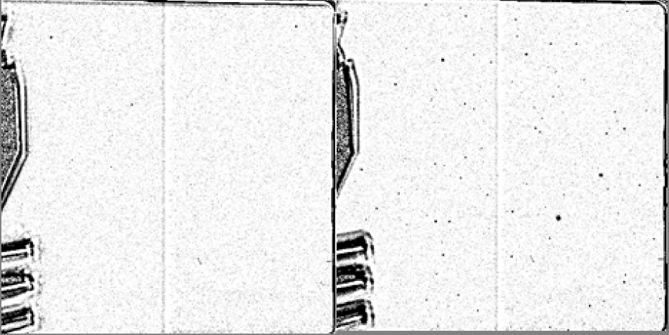
Figure 8: Comparison of two images taken with OSIRIS. They are 2-s exposure images at the Sloan $r$ filter, with a background level of $\sim$30,000 ADUs, of a DBF from our catalogue (left panel) and a BF from Azzaro catalogue (right panel) in the same region of the sky. The size of both fields is 8.5′$\times$8.5′. There is an evident improvement of our DBF with the one from the Azzaro catalogue. Note that the two apparent detections, both in the right-upper part in CCD1 (left side of the detector) and in left-bottom part in CCD2 (right side of the detector), are dust grain effects on the OSIRIS CCDs, and they do not correspond with any star in the field (they are also visible in the Azzaro field).

4 TESELA

In order to provide easy access to the DBF catalogue, we have incorporated it into TESELA, a WEB accessible tool, developed within the Spanish Virtual Observatory, which can be publicly accessed from http://sdc.cab.inta-csic.es/tesela.

The tool was implemented with a data base containing the new computed DBF regions from the USNO-B Catalog. Thus, through an user-friendly interface, the user can now perform a cone-search around a position in the sky in either the BF catalogue from Tycho-2 (see Paper I for a extended description) or the DBF catalogue from USNO-B Catalog. Through the search form for the DBF catalogue, users can select the $m_{\mbox{\scriptsize th}}$ and the search radius. The cone-search can be made in either equatorial or galactic coordinates.

TESELA presents the result of the cone-search in a table containing the same main properties of the DBFs presented in Tables LABEL:northDBFs. This table can be downloaded in CSV format for further use. TESELA also provides users with the possibility of visualizing the data. To do this, TESELA takes advantage of Aladin. Thanks to this connection with Aladin, we have provided the user with the full capacity and power of the VO. Using this Aladin window, users are allowed to load images and catalogues both locally and from the VO, having full access to the whole universe resident in the VO. This can be very helpful to determine the potential influence of relatively bright nebulae and extragalactic sources in the regions sought.

TESELA sends to Aladin the searching area, which is plotted in the first plane with a red circle, and the DBFs, which are shown by blue circles in a second layer. The size of the blue circles corresponds with the size of the DBFs. Finally, Aladin charges from the VO in a last layer the objects of NGC 2000.0 (Complete New General Catalogue and Index Catalogue of Nebulae and Star Clusters; Sinnott 1997). Note that, for obvious reasons, Solar system objects have been not considered, and they must be taken into account in order to make use of BF regions close to the ecliptic at a given date.

Table 3: Short list of selected DBFs.

(1)	(2)	(3)	(4)	(5)	(6)	(7)	(8)	(9)	(10)	(11)	(12)	(13)	(14)
RA	DEC	Gal Long	Gal Lat	$\rho$	$N_{*}$ with $m_{\mbox{\scriptsize R}}$		$m_{\mbox{\scriptsize R}}$		$F_{{\mbox{\scriptsize int}}}$	E(B-V) (mag)
(J2000)	(J2000)	(∘)	(∘)	(′)	$<$ 17.5	$<$ 22.0	Max	Min	(erg/s/cm2/A)	Center	Mean	Max.	Min.
Northern Hemisphere
00:06:57.17	+06:06:22.2	103.363380	–55.06648	5.03	14	86	20.56	16.13	8.45E–15	0.0738	(72$\pm$3)E–3	0.0771	0.0651
00:42:55.80	+41:20:04.2	121.215441	–21.50889	5.19	1	4	19.60	17.04	4.89E–16	0.6767	(58$\pm$10)E–2	0.7419	0.4284
01:08:41.88	+06:23:43.5	130.659924	–56.21711	5.18	5	97	20.31	16.61	4.38E–15	0.0252	(260$\pm$14)E–4	0.0288	0.0230
01:35:06.00	+14:33:23.4	138.518359	–46.98960	5.02	5	155	21.01	16.45	5.63E–15	0.0498	(49$\pm$3)E–3	0.0545	0.0451
02:01:10.30	+05:06:56.2	153.134220	–53.61670	5.08	3	83	19.78	17.06	3.82E–15	0.0425	(420$\pm$5)E–4	0.0428	0.0409
02:14:26.26	+14:01:23.9	151.573608	–44.18390	5.08	4	102	20.88	17.32	4.03E–15	0.1142	(113$\pm$7)E–3	0.1245	0.1007
02:56:21.26	+19:38:41.3	159.162056	–34.29385	5.27	0	17	20.16	18.46	6.24E–16	1.9877	(184$\pm$17)E–2	2.0707	1.4920
a03:33:31.70	+31:02:59.3	159.296833	–20.14533	5.03	0	21	19.85	18.73	5.86E–16	2.1341	(21$\pm$3)E–1	2.6959	1.5194
04:13:56.14	+28:08:33.0	168.217578	–16.42665	5.01	1	53	19.43	17.35	3.47E–15	1.6791	(169$\pm$6)E–2	1.7605	1.5595
a04:26:38.69	+24:39:00.4	172.908158	–16.71030	5.00	0	12	20.03	18.88	3.12E-16	1.1909	(118$\pm$10)E–2	1.3694	1.0021
04:45:42.65	+17:11:51.7	181.904567	–17.97142	5.28	27	222	20.76	16.07	2.13E–14	0.7981	(81$\pm$7)E–2	0.9400	0.6871
05:31:50.23	+12:37:23.5	192.273614	–11.30104	5.36	24	262	20.06	15.44	2.30E–14	1.9941	(20$\pm$3)E–1	2.5221	1.3798
05:47:22.73	+00:24:17.3	205.107319	–14.02273	5.03	0	37	19.55	17.53	1.83E–15	5.9760	(7$\pm$5)E–0	20.533	1.8988
06:24:09.29	+84:37:36.8	128.888339	+26.36465	5.19	31	220	20.79	15.13	2.99E–14	0.0694	(70$\pm$4)E–3	0.0772	0.0646
07:12:48.00	+56:17:40.6	160.555972	+25.16972	5.14	34	220	20.77	15.13	3.00E–14	0.0538	(538$\pm$6)E–4	0.0550	0.0526
07:36:47.76	+69:48:38.5	145.747848	+29.23289	5.34	34	226	20.61	15.30	2.68E–14	0.0289	(288$\pm$19)E–4	0.0320	0.0254
a07:48:36.72	+41:31:46.9	178.046803	+27.82759	5.36	33	197	20.38	15.15	2.38E–14	0.0439	(433$\pm$9)E–4	0.0456	0.0415
a08:52:36.48	+24:43:42.2	201.164237	+36.76278	5.22	9	139	20.74	16.66	8.47E–15	0.0323	(324$\pm$9)E–4	0.0338	0.0308
09:08:21.12	+74:08:07.4	138.975295	+35.13226	5.05	1	11	20.08	16.75	1.16E–15	0.0374	(365$\pm$10)E–4	0.0379	0.0339
09:33:13.20	+28:58:49.1	198.410292	+46.55147	5.05	6	103	19.61	16.50	5.81E–15	0.0178	(179$\pm$3)E–4	0.0184	0.0174
a09:58:19.68	+24:59:11.4	206.046838	+51.25283	5.20	5	104	19.97	17.36	4.83E–15	0.0446	(451$\pm$4)E–4	0.0460	0.0445
a10:30:25.20	+33:15:35.6	192.819814	+59.06935	5.11	0	95	20.28	18.02	3.13E–15	0.0162	(163$\pm$6)E–4	0.0175	0.0153
11:00:32.64	+22:03:55.4	218.197951	+64.34454	5.18	2	121	20.56	17.40	4.22E–15	0.0185	(183$\pm$5)E–4	0.0190	0.0168
a11:33:39.12	+13:26:35.9	246.056483	+67.25447	5.35	0	123	20.05	17.92	3.73E–15	0.0425	(424$\pm$11)E–4	0.0450	0.0410
11:54:07.92	+27:00:19.1	210.208221	+77.24893	5.03	1	134	20.89	17.20	4.52E–15	0.0257	(258$\pm$6)E–4	0.0273	0.0247
a12:41:44.40	+21:58:48.7	279.229077	+84.40000	5.10	0	186	19.96	17.64	6.28E–15	0.0293	(293$\pm$3)E–4	0.0298	0.0288
a12:56:12.72	+17:26:49.2	309.674643	+80.25619	5.01	1	127	20.75	17.12	5.19E-1-5	0.0308	(306$\pm$5)E–4	0.0318	0.0295
13:34:05.52	+24:56:42.0	22.478206	+80.17666	5.09	1	120	19.97	17.24	4.19E–15	0.0121	(120$\pm$5)E–4	0.0130	0.0110
a14:02:58.08	+35:11:28.7	65.170753	+72.74147	5.08	3	105	20.80	17.08	4.66E–15	0.0074	(79$\pm$5)E–4	0.0092	0.0074
14:22:46.32	+31:53:33.4	51.924015	+69.60795	5.02	3	184	20.89	16.52	6.65E–15	0.0127	(129$\pm$6)E–4	0.0141	0.0120
14:55:08.16	+43:30:10.4	74.358140	+60.18918	5.12	3	176	20.42	16.16	6.93E–15	0.0184	(184$\pm$4)E–4	0.0190	0.0176
15:31:05.76	+26:15:17.6	40.850494	+54.47989	5.12	9	147	20.43	16.10	8.70E–15	0.0612	(59$\pm$2)E–3	0.0623	0.0554
15:53:03.84	+40:32:32.3	64.708720	+50.46382	5.04	11	168	20.89	16.30	1.07E–14	0.0151	(155$\pm$9)E–4	0.0181	0.0144
16:30:00.96	+54:17:46.0	83.005830	+42.13076	5.06	21	182	20.66	15.33	1.69E–14	0.0135	(138$\pm$7)E–4	0.0155	0.0127
17:08:08.88	+58:40:45.1	87.474735	+36.23177	5.04	20	193	20.94	15.40	1.74E–14	0.0308	(305$\pm$16)E–4	0.0328	0.0274
17:25:15.36	+49:45:58.3	76.489792	+34.00138	5.10	26	206	20.72	15.18	2.31E–14	0.0273	(269$\pm$17)E–4	0.0300	0.0235
17:57:21.84	+72:56:51.7	103.750419	+29.79809	5.45	49	354	20.85	15.23	3.47E–14	0.0462	(454$\pm$6)E–4	0.0464	0.0439
18:28:53.76	+00:03:40.3	30.410269	+05.04183	5.22	2	110	19.14	16.41	7.45E–15	2.4687	(249$\pm$16)E–2	2.7710	2.2336
18:58:21.12	+04:21:07.8	37.592645	+00.44890	5.08	29	182	20.92	15.02	2.85E–14	13.295	(134$\pm$7)E–1	14.409	11.864
19:31:27.84	+22:20:38.4	57.250887	+01.73726	5.02	168	840	20.67	15.08	1.16E–13	3.1737	(310$\pm$11)E–2	3.3605	2.9270
20:15:04.80	+73:01:26.1	106.050051	+20.08241	5.14	55	386	20.69	15.16	4.37E–14	0.4431	(45$\pm$3)E–2	0.5103	0.3994
20:43:35.04	+67:49:17.4	102.720707	+15.32725	5.28	22	145	19.59	15.37	1.71E–14	0.7281	(71$\pm$4)E–2	0.7645	0.6330
20:59:12.72	+71:58:57.3	107.024821	+16.73696	5.59	29	241	20.30	15.61	2.14E–14	0.8555	(86$\pm$5)E–2	0.9680	0.7814
21:39:47.04	+70:20:33.7	108.072504	+13.22322	5.22	31	153	20.32	15.19	2.20E–14	1.1720	(111$\pm$6)E–2	1.2000	0.9856
a22:00:35.28	+76:30:26.6	113.410573	+16.90724	5.74	10	76	20.45	16.01	7.83E–15	1.2106	(118$\pm$2)E–2	1.2135	1.1261
22:21:37.92	+75:07:08.0	113.626695	+15.02513	5.04	14	142	20.92	16.03	1.04E–14	0.9246	(89$\pm$3)E–2	0.9255	0.8383
23:06:21.60	+00:30:48.0	76.217222	–52.55665	5.17	13	127	21.05	16.43	7.79E–15	0.0491	(490$\pm$15)E–4	0.0513	0.0463
23:22:00.72	+00:38:05.8	81.540479	–54.88397	5.02	4	104	20.64	16.06	5.38E–15	0.0403	(413$\pm$10)E–4	0.0441	0.0401
Southern Hemisphere
00:06:00.55	–16:15:04.3	76.546841	–74.86283	5.06	9	120	20.31	16.59	6.42E–15	0.0256	(253$\pm$5)E–4	0.0260	0.0244
00:37:40.03	–29:20:52.4	355.928862	–86.24195	5.05	3	127	21.86	17.08	4.04E–15	0.0196	(198$\pm$15)E–4	0.0230	0.0178
a00:59:31.22	–11:20:16.4	130.179575	–74.09580	5.13	0	75	20.37	17.57	2.91E–15	0.0317	(319$\pm$15)E–4	0.0354	0.0300
01:39:26.57	–32:50:56.8	244.671599	–78.14690	5.07	0	88	21.59	18.16	1.75E–15	0.0250	(249$\pm$5)E–4	0.0259	0.0241
02:09:49.25	–00:31:02.3	161.438111	–57.40772	5.31	0	129	21.23	18.28	4.37E–15	0.0271	(276$\pm$8)E–4	0.0293	0.0265
02:33:30.00	–13:25:28.2	188.126797	–62.51151	5.40	4	115	20.50	17.39	5.51E–15	0.0209	(207$\pm$4)E–4	0.0213	0.0196
03:08:50.59	–38:38:24.0	243.631348	–59.16465	5.17	4	123	20.86	17.06	4.17E–15	0.0219	(221$\pm$4)E–4	0.0231	0.0213
03:36:06.19	–20:58:11.3	212.743112	–52.07320	5.06	3	132	19.63	16.47	8.00E–15	0.0273	(274$\pm$8)E–4	0.0286	0.0258
04:02:24.96	–38:14:34.1	241.007990	–48.78829	5.00	9	121	21.93	16.15	6.99E–15	0.0051	(49$\pm$5)E–4	0.0062	0.0040
04:20:04.90	–15:16:00.5	210.263825	–40.297736	5.12	9	108	19.69	16.34	8.46E–15	0.0573	(56$\pm$3)E–3	0.0607	0.0502
05:01:40.01	–48:54:27.7	255.330888	–37.82428	5.04	16	159	21.92	15.71	1.20E–14	0.0117	(115$\pm$4)E–4	0.0123	0.0106
a05:41:55.18	–08:27:23.4	212.698747	–19.26914	5.03	0	15	19.69	18.27	5.90E–16	3.5394	(351$\pm$9)E–2	3.7273	3.2823
05:57:53.33	–13:37:16.7	219.388114	–17.91770	5.14	30	170	20.91	15.22	2.63E–14	0.5327	(55$\pm$5)E–2	0.6337	0.4742
09:05:29.28	–06:00:11.6	235.431491	+26.16744	5.10	29	161	19.40	15.01	2.86E–14	0.0281	(282$\pm$9)E–4	0.0299	0.0267
09:31:44.64	–01:45:46.9	235.687810	+33.96480	5.14	25	210	20.97	15.57	1.96E–14	0.0336	(336$\pm$9)E–4	0.0353	0.0315
10:10:14.16	–02:15:46.8	243.559329	+41.31715	5.02	24	238	20.47	16.03	1.70E–14	0.0408	(407$\pm$10)E–4	0.0428	0.0391
10:26:21.12	–00:07:38.5	244.926543	+45.76736	5.07	16	96	19.97	16.12	9.86E–15	0.0541	(552$\pm$19)E–4	0.0591	0.0527
11:05:33.84	–77:46:21.7	297.294235	–16.07566	5.18	3	99	20.98	16.37	4.39E–15	1.9375	(191$\pm$16)E–2	2.1494	1.5896
11:23:08.16	–01:42:10.3	263.002375	+54.17694	5.18	6	113	19.87	16.40	5.95E–15	0.0659	(66$\pm$3)E–3	0.0713	0.0611
11:58:47.28	–03:42:52.4	278.523051	+56.64133	5.01	5	132	19.82	16.63	6.91E–15	0.0294	(296$\pm$12)E–4	0.0326	0.0277
12:19:55.20	–00:09:51.1	286.137714	+61.67555	5.11	7	107	20.47	16.48	5.79E–15	0.0231	(234$\pm$4)E–4	0.0244	0.0229
12:55:39.12	–00:47:28.7	305.180788	+62.06203	5.05	12	94	20.98	16.43	6.25E–15	0.0175	(182$\pm$9)E–4	0.0203	0.0168
13:38:06.24	–10:44:17.5	321.123566	+50.47792	5.07	7	156	19.82	16.12	9.47E–15	0.0810	(80$\pm$4)E–3	0.0856	0.0709
14:00:15.84	–03:33:17.4	334.006917	+55.10961	5.09	13	178	20.18	16.06	1.20E–14	0.0462	(47$\pm$2)E–3	0.0520	0.0435
14:37:44.40	–05:14:50.0	345.355145	+48.67014	5.18	19	160	21.72	16.01	1.18E–14	0.0719	(724$\pm$3)E–4	0.0729	0.0718
15:04:41.52	–03:47:04.5	354.237024	+45.39982	5.06	22	152	20.51	15.59	1.81E–14	0.1748	(173$\pm$7)E–3	0.1839	0.1608
15:42:55.44	–34:06:39.6	338.915415	+16.51832	5.02	8	77	19.05	16.36	7.81E–15	0.8542	(861$\pm$15)E–3	0.9031	0.8371
a15:53:31.92	–04:42:22.8	4.103063	+35.73414	5.54	0	41	20.95	18.08	1.26E–15	0.9739	(93$\pm$6)E–2	1.0348	0.8230
16:27:41.76	–24:45:20.9	352.989963	+16.46125	5.08	0	22	20.80	18.89	5.13E–16	2.3699	(23$\pm$5)E–1	3.4392	1.6456
16:50:49.68	–15:22:04.8	4.219387	+18.07220	5.07	0	72	19.99	18.19	2.70E–15	1.7061	(169$\pm$11)E–2	1.8476	1.5248
17:34:12.72	–25:23:06.0	1.665072	+04.03459	5.48	21	282	19.73	15.43	2.73E–14	2.6267	(261$\pm$5)E–2	2.6868	2.4711
18:04:55.92	–24:17:11.8	6.191747	–01.37869	5.29	0	2	17.73	17.64	3.11E–16	7.8239	(8$\pm$2)E–0	12.452	5.7035
a18:28:03.12	–03:49:55.9	26.846166	+03.43861	5.77	0	30	20.16	18.08	1.44E–15	10.819	(10$\pm$5)E–0	23.146	3.8047
19:04:04.08	–37:17:30.1	359.760820	–18.377007	5.01	11	144	20.83	16.10	9.96E–15	0.9750	(96$\pm$5)E–2	1.0277	0.8332
19:32:23.76	–78:26:14.3	315.912763	–28.58364	5.57	38	191	20.08	15.07	2.69E–14	0.4874	(48$\pm$4)E–2	0.5469	0.4208
19:52:11.04	–81:06:33.8	312.761609	–29.113235	5.51	38	189	20.87	15.14	2.58E–14	0.7702	(73$\pm$8)E–2	0.8514	0.5749
21:05:41.76	–27:46:21.0	18.361528	–40.37909	5.24	43	302	20.23	15.00	3.33E–14	0.1084	(107$\pm$2)E–3	0.1113	0.1026
21:22:02.16	–07:17:39.3	44.676556	–36.66431	5.01	15	166	21.00	15.63	1.32E–14	0.2486	(241$\pm$6)E–3	0.2497	0.2243
22:07:12.72	–19:14:43.4	35.818926	–51.61918	5.02	12	145	21.13	16.38	1.01E–14	0.0260	(258$\pm$10)E–4	0.0286	0.0244
a22:41:36.24	–13:28:34.7	50.650654	–56.77675	5.31	16	151	21.00	16.07	1.01E–14	0.0495	(497$\pm$17)E–4	0.0527	0.0464
22:58:27.84	–47:34:36.8	342.524449	–59.94059	5.25	8	155	21.88	16.33	6.34E–15	0.0097	(102$\pm$12)E–4	0.0130	0.0086
a23:40:51.12	–03:53:58.6	83.895230	–61.30129	5.25	10	90	20.65	16.62	6.10E–15	0.0373	(374$\pm$12)E–4	0.0399	0.0359
Note: a DBF validated and regularly used at the GTC.

Table 3: continued.

References

- Bonnarel et al. (2000) Bonnarel, F., Fernique, P., Bienaymé, O., et al. 2000, A&AS, 143, 33
- Barron et al. (2008) Barron J. T., Stumm C., Hogg D. W., Lang D., Roweis S., 2008, AJ, 135, 414
- Cardiel et al. (2011) Cardiel N., Jiménez-Esteban F. M., Alacid J. M., Solano E., Aberasturi M., 2011, MNRAS, 417, 3061
- Cepa et al. (2000) Cepa, J., et al. 2000, Proc. SPIE, 4008, 623
- Delaunay (1934) Delaunay B., 1934, Sur la sphère vide, Bull. Acad. Sci. USSR, 793–800
- Gilliland (1992) Gilliland R.L., 1992, Details of Noise Sources and Reduction Processes. In: Howell S.B. (ed.) ASP Conf. Ser. 23, Astronomical CCD Observing and Reduction Techniques, p. 68
- Høg et al. (2000) Høg E., et al., 2000, A&A, 355, L27
- Monet et al. (2003) Monet D. G., et al., 2003, AJ, 125, 984
- De Muth (2006) De Muth J.E., 2006, Basic Statistics and Pharmaceutical Statistical Applications, 2nd Edition, Chapman & Hall/CRC, p. 577
- Schlegel, Finkbeiner, & Davis (1998) Schlegel D. J., Finkbeiner D. P., Davis M., 1998, ApJ, 500, 525
- Sinnott (1997) Sinnott, R. W. 1997, VizieR Online Data Catalog, 7118, 0