On the Weak Coupling Limit for Massive Yang-Mills

Daniele Bettinelli^a, and Ruggero Ferrari^a,b,

Abstract: For small values of the gauge coupling constant, we compare the densities of the energy of the vacuum and of the order parameter, evaluated in the lattice Monte Carlo simulation and in the perturbative field theory at two loop (Minkowski). The continuum calculation allows a very good fit of the simulation results, away from the phase transition line. This confirms the conjecture that the lattice provides a regularization of the (nonrenormalizable) massive Yang-Mills and moreover it shows the physical meaning of the parameters used in the simulation.

1 Introduction

In a recent paper [1], a lattice gauge theory for massive $SU(2)$ Yang-Mills in dimension four has been proposed. The completely gauge independent analysis shows the presence of a Transition Line (TL) in the parameter space $(m^{2}\sim 1/\beta)$, which seems to indicate a phase transition (but it might also be a cross over) for large $\beta$, starting from $\beta\sim 2.2$. The large $\beta$ limit value of $\beta m_{c}^{2}$, where $m_{c}^{2}$ is the critical value of $m^{2}$ on the TL, is in good agreement with the critical point of the nonlinear sigma model in four dimensions quoted in Ref.[2], namely $0.65\pm 0.04$.

The above-mentioned lattice gauge model has been studied previously (see [3]-[10]) as an example of Higgs mechanism with a frozen length. In Ref. [1] we showed that it is the perfect tool for the simulation of the massive Yang-Mills (i.e. with a mass à la Stückelberg). The phase TL has an end-point around ( $\beta\sim 2.2,\,\,m^{2}\sim 0.381$): for smaller $\beta$ there is a smooth transition from one phase to the other, while for larger $\beta$ there are numerical indications of singularities in the derivatives with respect to $m^{2}$ and to $\beta$ of the energy and of the order parameter (i.e. the $\ln m^{2}$ derivative of the free energy).

The lattice model turns out to be extremely interesting by itself because of the states structure, the dynamical content, the limit of small gauge coupling, the complexity of the phase diagram in the parameter space $(\beta,m^{2})$. In this paper we want to compare the lattice model with the Yang-Mills gauge theory where a mass à la Stückelberg is introduced. The latter model is nonrenormalizable, but we have devised a method to make a respectable physical theory out of it ([11]-[15]). The comparison of the two models, via analytic continuation, can provide interesting results, if we find some physical quantities where they are expected to give identical results. Global quantities might be good candidates in order to compare the two models and thus to identify the physical meaning of the lattice parameters.

To this end, we investigate on the small gauge coupling behavior, i.e. large $\beta$, of some global observables such as densities of the “energy of the vacuum” and of the order parameter

$${\cal E}_{L}=-\frac{1}{N}\beta\frac{\partial}{\partial\beta}\ln Z_{L}$$

$${\mathfrak{C}}_{L}=-\frac{1}{N}m^{2}\frac{\partial}{\partial m^{2}}\ln Z_{L}\,,$$ (1)

where $N$ is the number of sites and $Z_{L}$ the partition function . It should be noticed that in Ref. [1] the order parameter is defined as

$$1-\frac{\mathfrak{C}_{L}}{m^{2}D\beta},$$ (2)

in order to put in evidence its behavior for $m^{2}=0$ and $m^{2}\to\infty$. Here these properties are not relevant.

In this work we discuss two important questions: i) to understand the phenomenological meaning of the parameters $\beta$ and $m^{2}$ (in the naive continuum limit, $a\to 0$ , $\beta=4g^{-2}$ and $ma^{-1}$ is the mass of the vector mesons); ii) to compare the lattice regularization of the theory with the continuum Minkowskian formulation of massive Yang-Mills theory proposed in Refs. [11] and [12]. Regarding i), we want to find the scales necessary in order to interpret the otherwise dimensionless parameter $m$. For the point ii), we assume that the finite lattice artifacts are not relevant quantitatively for the global quantities of eq. (1).

The transition from Euclidean to Minkowskian quantities is performed in the usual conventional way: $\exp(iS_{M})$ is the weight in the path integral and the arrow of time (i.e. anticlockwise Wick rotation) is chosen in order to match the edge-of-the-wedge theorem [16].

In the subtraction procedure [13] - [15] a scale $\Lambda$ of the radiative correction is introduced, then it is natural to look for a correspondence implemented by the mapping

$$g^{2}=f(\beta,m^{2})$$

$$\frac{M^{2}}{\Lambda^{2}}=s(\beta,m^{2})$$

$$Ma=t(\beta,m^{2}),$$ (3)

where the parameters $g,M$ are the field theory coupling constant and mass respectively, while $a$ is the ”lattice spacing”, i.e. a length introduced for dimensional reasons. Eqs. (3) show that the mapping of the continuum field theory onto the lattice implies a choice of a surface in the three-dimensional space spanned by the dimensionless parameters ($g$, $Ma$ and $\Lambda a$). The convenience of these choices might be sustained and tested on the physical observables to be compared.

The fit indicates that far from $m_{c}^{2}$ ($m^{2}>m_{c}^{2}$) and for large $\beta$ the field theory predictions at two-loop describe very well the lattice simulation data and moreover $a\sim M^{-1}$, $m\sim\Lambda^{-1}M$ and the Yang-Mills coupling constant $g$ is a mildly decreasing function of $\beta$ (the lattice parameter) with $g^{2}\sim 4/\beta$ at $\beta=20$.

2 Massive Yang-Mills in Field Theory (Minkowski)

In the continuum quantum field theory the classical action is

$$S_{M}=\frac{\Lambda^{(D-4)}}{g^{2}}\int d^{D}x\,\Big{(}-\frac{1}{4}G_{a\mu\nu}[A]G^{\mu\nu}_{a}[A]+\frac{M^{2}}{2}(A_{a\mu}-F_{a\mu})^{2}\Big{)}\,.$$ (4)

The path integral functional $Z_{M}$ is obtained by integration over the fields $A_{\mu}$ and $\Omega\in SU(2)$, where ($\tau$ are the Pauli matrices)

$$\Omega=\phi_{0}+i\tau_{j}\phi_{j},\qquad F_{\mu}\equiv i\Omega\partial_{\mu}\Omega^{\dagger}.$$ (5)

The constraint on $\Omega$

$$1=\phi_{0}^{2}+\vec{\phi}^{2}$$ (6)

renders the theory in eq. (4) nonrenormalizable. The procedure of subtraction of the infinities in perturbation theory is described in detail in Ref. [11]. Here we account only for the final practical rule: only pure pole subtraction is performed on the dimensionally regularized Feynman amplitudes normalized by

$$\Lambda^{(4-D)}{\cal A}.$$ (7)

No additional finite adjustment is allowed, e.g. on-shell normalization.

We use Landau gauge because it is very useful in a massive theory, where the massless modes are all unphysical. The absence of the massless modes contributions provides a good check for the calculation of the physical observables.

The “energy of the vacuum” per hypercube $a^{4}$ is then given by the path integral mean value $\langle\rangle_{M}$

$${\cal E}_{M}(g,M,\Lambda,a)=\Big{\langle}-\frac{a^{4}}{g^{2}}\Big{(}-\frac{1}{4}G_{a\mu\nu}[A]G^{\mu\nu}_{a}[A]+\frac{M^{2}}{2}A_{a\mu}^{2}\dots\Big{)}\Big{\rangle}_{M},$$ (8)

where $\dots$ stand for the counterterms and for the terms of the classical action depending on the unphysical fields as $\Omega$ and Faddeev-Popov ghosts $c,\bar{c}$. The full expression is given in Ref. [11].

The ${\cal O}(g^{0})$ of ${\cal E}_{M}$ is zero. This result can be proved formally by applying the operator $g\frac{\partial}{\partial g}$ to $Z_{M}$ before and after the rescaling of the field $A_{\mu}\to gA_{\mu}$. The ${\cal O}(g^{2})$ part amounts to the evaluation of the graphs in Fig. 1; i.e. after rescaling

$${\cal E}_{M}=\Big{\langle}a^{4}\frac{g}{2}\frac{\partial}{\partial g}\Big{(}-\frac{1}{4}G_{a\mu\nu}[A]G^{\mu\nu}_{a}[A]+\frac{M^{2}}{2}A_{a\mu}^{2}\dots\Big{)}\Big{\rangle}_{M}.$$ (9)

Figure 1: The Goldstone boson lines are dashed. The Faddeev-Popov propagators are dotted.

2.1 Two Loop Amplitude

A straightforward calculation gives the Feynman amplitude properly normalized [13] by the factor $\Lambda^{(4-D)}$

$${\cal E}_{1M}=-\frac{3}{2}a^{4}g^{2}\Bigg{[}3\Big{(}D-\frac{5}{4}\Big{)}M^{2}I_{2}[M]-\Big{(}D^{2}-4D+\frac{15}{4}\Big{)}A_{0}[M]^{2}\Bigg{]}.$$ (10)

The integrals are defined by

$$I_{2}[M]=\int_{M}\frac{d^{D}q}{(2\pi)^{D}}\int_{M}\frac{d^{D}p}{(2\pi)^{D}}\frac{\Lambda^{(8-2D)}}{(q^{2}-M^{2})(p^{2}-M^{2})[(q+p)^{2}-M^{2}]}$$

$$A_{0}[M]=\int_{M}\frac{d^{D}q}{(2\pi)^{D}}\frac{\Lambda^{(4-D)}}{(q^{2}-M^{2})}.$$ (11)

It should be noticed that all contributions by the massless modes cancel out (no contributions from the unphysical sector).

The tadpole integral is

$$\!\!\!\!\!\!\!\!\!\!\!\!\!\!\!\!\!\!\!A_{0}[M]=i\frac{M^{2}}{(4\pi)^{2}}\Bigg{[}-\frac{2}{D-4}-\ln\Delta$$

$$~{}~{}~{}~{}~{}~{}~{}~{}~{}~{}~{}~{}~{}-\frac{1}{4}(D-4)\Big{(}\ln^{2}\Delta+1+\frac{\pi^{2}}{6}\Big{)}\Bigg{]}+{\cal O}\big{(}(D-4)^{2}\big{)},$$ (12)

where

$$\Delta=\frac{e^{(\gamma-1)}M^{2}}{4\pi\Lambda^{2}}.$$ (13)

Consequently, one gets

$$A_{0}[M]^{2}=-\frac{M^{4}}{(4\pi)^{4}}\Bigg{[}\frac{4}{(D-4)^{2}}+\frac{4}{D-4}\ln\Delta+1+\frac{\pi^{2}}{6}+2\ln^{2}\Delta\Bigg{]}.$$ (14)

The two-loop integral can be found in the literature (see Ref. [17])

$$\!\!\!\!\!\!\!\!\!\!\!\!\!\!\!\!\!\!\!\!\!I_{2}[M]=3\frac{M^{2}}{(4\pi)^{4}}\Bigg{[}-\frac{2}{(D-4)^{2}}+\frac{1}{D-4}\Big{(}1-2\ln\Delta\Big{)}$$

$$~{}~{}~{}~{}~{}~{}~{}~{}~{}~{}-\Big{(}-\ln\Delta+\frac{\pi^{2}}{12}+\frac{3}{2}+\ln^{2}\Delta\Big{)}+\frac{2}{\sqrt{3}}Cl_{2}\Big{(}\frac{\pi}{3}\Big{)}\Bigg{]},$$ (15)

where the Euler-Mascheroni constant and the Clausen function are

$$\gamma=0.5772156649$$

$$Cl_{2}\Big{(}\frac{\pi}{3}\Big{)}=1.014941606.$$ (16)

Finally, the contributions of the graphs in Fig. 1 add up to

$$\!\!\!\!\!\!\!\!\!\!\!\!\!{\cal E}_{1M}=-\frac{3}{2}a^{4}g^{2}\frac{M^{4}}{(4\pi)^{4}}\Bigg{[}-\frac{69}{2}\frac{1}{(D-4)^{2}}-\frac{1}{(D-4)}\Big{(}-\frac{91}{4}+\frac{69}{2}\ln\Delta\Big{)}$$

$$~{}~{}~{}~{}-\frac{163}{8}+\frac{91}{4}\ln\Delta-\frac{69}{4}\ln^{2}\Delta-\frac{23}{16}\pi^{2}+\frac{99}{2\sqrt{3}}Cl_{2}\Big{(}\frac{\pi}{3}\Big{)}\Bigg{]}.$$ (17)

2.2 Contribution of the Counterterms

In order to evaluate the contribution of the counterterms, we use the results of Ref. [12] eq. (29)

$$\!\!\!\!\!\!\!\!\!\!\!\!\widehat{\Gamma}^{(1)}\equiv\int d^{D}x\,\,\widehat{\gamma}^{(1)}(x)$$

$$=\frac{\Lambda^{(D-4)}}{(4\pi)^{2}}\frac{1}{D-4}\int d^{D}x\Big{[}\frac{17}{4}\Big{(}\partial_{\mu}A_{a\nu}\partial^{\mu}A_{a}^{\nu}-(\partial A_{a})^{2}\Big{)}+\frac{3}{2}M^{2}A_{a}^{2}\Big{]}.$$ (18)

Then the contribution of the counterterms is

$$\!\!\!\!\!\!\!\!\!\!\!\!{\cal E}_{2M}=-i\frac{a^{4}g^{2}M^{2}}{(4\pi)^{2}}\frac{D-1}{D-4}\frac{69}{4}A_{0}[M^{2}]$$

$$=-\frac{3}{2}\frac{a^{4}g^{2}M^{4}}{(4\pi)^{4}}\Bigg{[}\frac{69}{(D-4)^{2}}+\frac{1}{D-4}\Big{(}23+\frac{69}{2}\ln\Delta\Big{)}+\frac{23}{2}\ln\Delta$$

$$~{}~{}~{}~{}~{}~{}~{}~{}~{}~{}~{}~{}~{}~{}~{}~{}~{}~{}~{}+\frac{69}{8}\Big{(}\ln^{2}\Delta+1+\frac{\pi^{2}}{6}\Big{)}\Bigg{]}.$$ (19)

The final result for the energy of the vacuum to order ${\cal O}(g^{2})$ is

$$\!\!\!\!\!\!\!\!\!\!\!\!\!\!\!\!\!\!\!\!\!{\cal E}_{M}={\cal E}_{1M}+{\cal E}_{2M}=-\frac{3}{2}a^{4}g^{2}\frac{M^{4}}{(4\pi)^{4}}\Bigg{[}\frac{69}{2}\frac{1}{(D-4)^{2}}+\frac{183}{4}\frac{1}{(D-4)}$$

$$~{}~{}~{}~{}~{}~{}~{}~{}~{}~{}~{}~{}~{}~{}-\frac{69}{8}\ln^{2}\Delta+\frac{137}{4}\ln\Delta-\frac{47}{4}+\frac{99}{2\sqrt{3}}Cl_{2}\Big{(}\frac{\pi}{3}\Big{)}\Bigg{]}.$$ (20)

Notice that the singular part has no dependence on $\Delta$. The finite part is then

$${\cal E}_{M}=-\frac{3}{2}a^{4}g^{2}\frac{M^{4}}{(4\pi)^{4}}\Bigg{[}-\frac{69}{8}\ln^{2}\Delta+\frac{137}{4}\ln\Delta-\frac{47}{4}+\frac{99}{2\sqrt{3}}Cl_{2}\Big{(}\frac{\pi}{3}\Big{)}\Bigg{]}.$$ (21)

2.3 The Order Parameter

The order parameter at ${\cal O}(g^{0})$ is given by

$${\mathfrak{C}}_{M}^{(0)}=-a^{4}\Big{\langle}\frac{M^{2}}{2}(A_{a\mu}-F_{a\mu})^{2}\Big{\rangle}_{M}^{(0)}=\frac{3}{2}\frac{a^{4}M^{4}}{(4\pi)^{2}}\Big{(}\frac{6}{D-4}+3\ln\Delta+2\Big{)},$$ (22)

where the path integral mean value is taken with the free part of the action. The ${\cal O}(g^{2})$ can be easily evaluated with a trick. We use the fields scaled in such a way that the coupling constant appears only in the interacting part of the action. Then we have the identity

$${\mathfrak{C}}_{M}^{(2)}=\frac{g}{2}\frac{\partial}{\partial g}{\mathfrak{C}}_{M}^{(2)}=i\frac{M^{2}}{N}\frac{\partial}{\partial M^{2}}\frac{g}{2}\frac{\partial}{\partial g}\ln Z_{M}=-M^{2}\frac{\partial}{\partial M^{2}}{\cal E}_{M}.$$ (23)

Thus we use the expression in eq. (20)

$$\!\!\!\!\!\!\!\!\!\!\!\!\!\!\!{\mathfrak{C}}_{M}^{(2)}=\frac{3}{2}g^{2}\frac{a^{4}M^{4}}{(4\pi)^{4}}\Bigg{[}69\frac{1}{(D-4)^{2}}+\frac{183}{2}\frac{1}{D-4}$$

$$~{}~{}~{}~{}~{}~{}~{}~{}~{}~{}~{}~{}~{}~{}-\frac{69}{4}\ln^{2}\Delta+\frac{205}{4}\ln\Delta+\frac{43}{4}+33\sqrt{3}Cl_{2}\Big{(}\frac{\pi}{3}\Big{)}\Bigg{]}.$$ (24)

We notice that once again the singular terms depending on $\Delta$ cancel out in the final amplitudes.

3 Euclidean-Minkowskian Correspondence

The correspondence is established by requiring that the observables have the same value. The mapping is obtained by the substitution

$$x_{4}=-ix_{0}$$

$$A_{4}=iA_{0}$$ (25)

and by performing an anticlockwise Wick rotation on the $x_{0}$ integration (to match the statement of the edge-of-the-wedge theorem [16]). The generating functionals are obtained by summing over the field configurations with the weights

$$e^{-S_{E}}$$

$$e^{iS_{M}}\textsl{}$$ (26)

for the Euclidean $\langle\rangle_{E}$ and Minkowskian $\langle\rangle_{M}$ mean values, where $S_{E}$ is the Euclidean action obtained from $S_{M}$ by using the mapping in eq. (25). Then we use the correspondence

$$\!\!\!\!\!\!\!\!\!\!\!\!\!\!\!\!\!\!\!\!\!\!\!\Big{\langle}\Big{(}\dots\phi(x_{j})\dots A_{\mu_{k}}(x_{k})\dots\Big{)}\Big{\rangle}_{M}\Big{|}_{\!\!\!\!\tiny{\begin{array}[]{l}\\ x_{0}=i\,x_{4}\\ A_{0}=-iA_{4}\end{array}}}\!\!\!\!\!\!\!\!\!\!\!\!=\Big{\langle}\Big{(}\dots\phi(x_{j})\dots A_{\mu_{k}}(x_{k})\dots\Big{)}\Big{\rangle}_{E}.$$ (30)

In the Minkowski case the field theory is made finite by the procedure briefly outlined at the beginning of Sec. 2. For the Euclidean formulation, we want to investigate the possibility to approximate the amplitudes by a gauge lattice model given by an appropriate action $S_{L}$ introduced in Ref. [1] and discussed later on. In fact, the paper is devoted to this comparison by considering the global quantities ${\cal E}_{L}$ and ${\mathfrak{C}}_{L}$ in lattice gauge theory in the limit of weak coupling ($\beta\gg 1$), where perturbation theory can be used for the theory in the continuum.

4 The Lattice Model

The action in eq.(4) is invariant under $g_{\scriptstyle{\scriptstyle{L}}}(x)\in SU(2)_{L}$ local-left and $g_{\scriptstyle{R}}\in SU(2)_{R}$ global-right transformations. On the lattice, one can implement the same transformations by using link variables $U(x,\mu)$ and site variables $\Omega(x)\in SU(2)$. We have

$$\!\scriptstyle{SU(2)_{L}}\left\{\begin{array}[]{l}\Omega^{\prime}(x)=g_{L}(x)\Omega(x)\\ U^{\prime}(x,\mu)=g_{L}(x)U(x,\mu)g^{\dagger}_{L}(x+\mu)\end{array}\right.\!\!,~{}\,\,\scriptstyle{SU(2)_{R}}\left\{\begin{array}[]{l}\Omega^{\prime}(x)=\Omega(x)g_{R}^{\dagger}\\ U^{\prime}(x,\mu)=U(x,\mu)\end{array}\right.\!.$$ (35)

The lattice model is constructed by assuming the same invariance properties. The nearest neighbor interaction is required to map naïvely into the action (4) for zero lattice spacing. The link variable is taken to be

$$U(x,\mu)\simeq\exp(-iaA_{\mu}(x)).$$ (36)

Thus the action is

$$S_{L}=\!\!\frac{\beta}{2}\,\,{\mathfrak{R}e}\sum_{\Box}Tr\big{\{}1-U_{\Box}\big{\}}+\frac{\beta}{2}m^{2}{\mathfrak{R}e}\sum_{x\mu}Tr\Bigl{\{}1-\Omega(x)^{\dagger}U(x,\mu)\Omega(x+\mu)\Bigr{\}},$$ (37)

where the sum over the plaquette is the Wilson action [18] and the mass term has the (Euclidean) continuum limit

$$\frac{\beta}{2}M^{2}a^{2}{\mathfrak{R}e}\sum_{x\mu}Tr\Bigl{\{}1-\Omega(x)^{\dagger}U(x,\mu)\Omega(x+\mu)\Bigr{\}}$$

$$\to\frac{M^{2}}{g^{2}}\int d^{4}x\,\,Tr\,\Big{\{}(A_{\mu}-i\Omega\partial_{\mu}\Omega^{\dagger})^{2}\Big{\}},$$ (38)

to be compared with the corresponding term in eq. (4).

5 The Lattice Simulation

The partition function is obtained by summing over all configurations given by the link variables and the $SU(2)$-valued field $\Omega$

$$Z_{L}[\beta,m^{2},N]=\sum_{\{U,\Omega\}}e^{-S_{L}},$$ (39)

where $N$ is the number of sites.

In principle the integration over $\Omega(x)$ is redundant, since by a change of variables ($U_{\Omega}(x,\mu):=\Omega(x)^{\dagger}U(x,\mu)\Omega(x+\mu))$ we can factor out the volume of the group. $Z_{L}[\beta,m^{2},N]$ becomes

$$\!\!\!\!\!\!\Big{[}\sum_{\{\Omega\}}\Big{]}\sum_{\{U\}}\exp-\frac{\beta}{2}\Big{(}{\mathfrak{R}e}\sum_{\Box}Tr\big{\{}1-U_{\Box}\big{\}}+m^{2}{\mathfrak{R}e}\sum_{x\mu}Tr\Bigl{\{}1-U(x,\mu)\Bigr{\}}\Big{)}.$$ (40)

However, in eq.(39) we force the integration over the gauge orbit $U_{\Omega}$ by means of the explicit sum over $\Omega$. In doing this, we gain an interesting theoretical setup of the model; in practice, our formalism is fully gauge invariant. Moreover, by forcing the integration over the gauge orbit $U_{\Omega}$ we get results which are less noisy than those obtained by using only the integration over the link variables in eq.(40).

5.1 Numerical results

The numerical analysis of the model [1] shows the existence of a line (Fig.2) where the functions $\cal E$ and $\mathfrak{C}$ have inflection points in $m^{2}$ and $\beta$. In the region $\beta>2.2$ the line separates the unconfined phase with vector mesons from the phase where confinement may occur.

Figure 2: The transition line. The arrow marks the position of the end point. In the figures of the present paper the statistical errors are not displayed since they are too small to be shown.

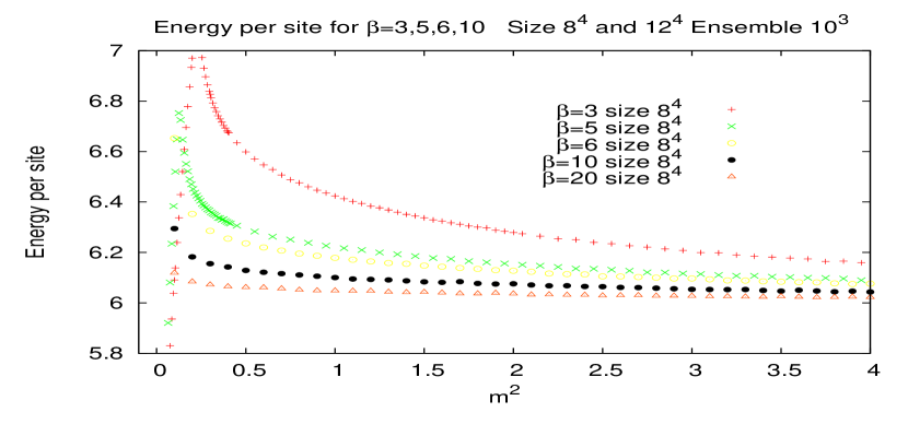
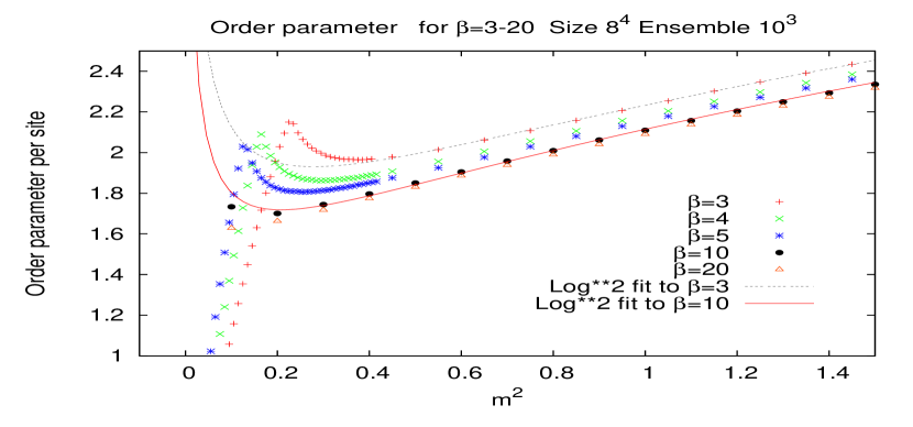
In the region of weak coupling (large $\beta$) and above the transition line we have evaluated the energy of the vacuum $\cal E$ and the order parameter $\mathfrak{C}$ per site for $m^{2}=0.1\dots 8$. We have used a cubic lattice with size $8^{4}$ and $12^{4}$. No difference could be spotted in the results for the two choices. We have taken $10^{3}$ measures separated by $15$ updatings. For $\beta=10$ we have performed $10^{4}$ measures in order to reduce the statistical errors, but no appreciable improvement was observed. Some results are given in Figs.3 and 4. It is very interesting that both these global quantities converge for large $m^{2}$ to values independent from $\beta$. From eq. (37) one would expect a strong dependence from the mass. From both figures, we see that near the transition line the dependence on $\beta$ becomes strong. In Fig. 4 we show a simple fit of the data at $\beta=3,10$ with polynomials of second degree in $\ln(m^{2})$.

Figure 3: Energy per site at $\beta=3,5,6,10,20$ as function of $m^{2}$.

Figure 4: Order parameter ${\mathfrak{C}}$ per site at $\beta=3,4,5,10,20$ as function of $m^{2}$.

6 The Fit

In the present Section we try a fit of the analytic results of Section 2 to the data obtained by simulation in Section 5. We use a simplified form of the mapping (3)

$$g^{2}=f(\beta)$$

$$\frac{M^{2}}{\Lambda^{2}}={m^{2}}\,{s(\beta)}$$

$$aM=t(\beta),$$ (41)

where the numerical values of $f,s,t$ are determined by the fit. The results of Section 2 become

$${\cal E}_{M}^{(2)}=\frac{3}{2}g^{2}\frac{a^{4}M^{4}}{(4\pi)^{4}}8.625\Big{[}\Big{(}\ln m^{2}+\ln s-4.939\Big{)}^{2}-5.943\Big{]}+e_{0}$$

$${\mathfrak{C}}_{M}^{(0)}=\frac{3}{2}\frac{a^{4}M^{4}}{(4\pi)^{2}}8.625\Big{[}0.348\Big{(}\ln m^{2}+\ln s-2.954\Big{)}+0.232\Big{]}$$

$${\mathfrak{C}}_{M}^{(2)}=\frac{3}{2}g^{2}\frac{a^{4}M^{4}}{(4\pi)^{4}}8.625\Big{[}-2\Big{(}\ln m^{2}+\ln s-4.439\Big{)}^{2}+12.386\Big{]}.$$ (42)

The parameters are fitted according to the following steps: i) first we fit the energy, since it is ${\cal O}(g^{2})$; ii) then we enter the parameters obtained by i) ($[g^{2}(aM)^{4}]$ and $\ln s$) into ${\mathfrak{C}}_{M}$ and we perform the best fit for

$${\mathfrak{C}}_{M}^{(0)}+{\mathfrak{C}}_{M}^{(2)}+e_{1}$$ (43)

on a range of $m^{2}$ far from the transition line. The output of the fit procedure are the parameters $g^{2},aM,\ln s,e_{0},e_{1}$. For convenience, we shall display the quantity

$$\beta_{\rm fit}\equiv\frac{4}{g^{2}},$$ (44)

where $g^{2}$ is the value obtained from the fit, in order to have a prompt comparison with the lattice parameter $\beta$.

The strategy is dictated by the fact that the direct fit of the order parameter does not determine properly the values of $aM$ and $\ln s$, since these last parameters have weak effect in comparison with the ${\cal O}(g^{0})$ term. Thus it is better to work at first with a ${\cal O}(g^{2})$ quantity: the vacuum energy. However, the results of the first step depend strongly on the range of $m^{2}$; therefore, we choose the interval that yields a common value for $\ln s$ according to the parameterization of eq. (41). The interval is reported in Table 1 in the second column.

6.1 Fit of the Vacuum Energy

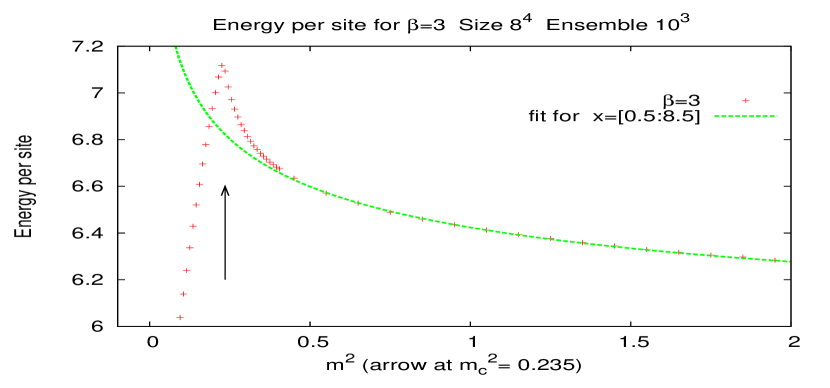
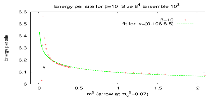
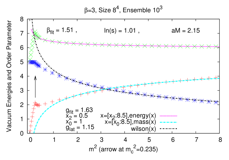
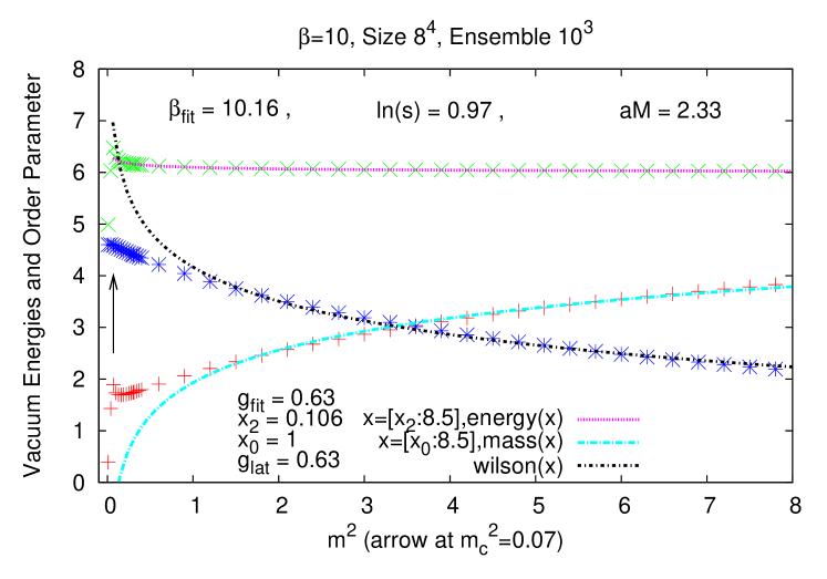
We perform the fit of the total energy ${\cal E}_{M}^{(2)}$ of eq. (42) for $\beta=3,4,5,6,7,8,9,$ $10,20$. Figs. 5 and 6 give a reasonable account of the match between lattice gauge theory and the field theory calculation with our subtraction procedure. In Table 1 we list some of the data of the fit: in particular $\ln s$, the $m^{2}$ interval and $\chi^{2}$ (which is very small). It should be noticed that $aM$ and $g^{2}$ can be determined only by using the fit of the order parameter, since the energy expression contains only the product $[g^{2}(aM)^{4}]$.

Figure 5: Fit of the field theory prediction (eq. (42)) to the lattice data for $\beta=3$. The parameters are $g^{2}(aM)^{4}$, $\ln s$, $e_{0}$.

Figure 6: See caption of Fig. 5 for $\beta=10$.

6.2 Combined Fit of the Vacuum Energy and the Order Parameter

In the second step we fit the order parameter; thus we find the value of $g^{2}$ and $aM$. The results of the procedure are listed in Table 2 ($aM$, $\beta_{fit}=4/g^{2}$ and $\chi^{2}$ of the fit). In Figs. (7) and (8) we depict the results of the fit procedure for the values $\beta=3,10$. The plots include also the value of the Wilson action of the vacuum (${\cal E}-{\mathfrak{C}}$). The figures show explicitly that the fit procedure intentionally excludes the region near the transition line (at $m_{c}^{2}$).

The numerical results show that the field theory two-loop calculation of the energy of the vacuum and the order parameter provides a good fit of the lattice data on the surface given by the parametric equations (41). The data in Tables 1, 2 indicate that $aM$ is almost constant for high values of $\beta$. Instead $\beta_{fit}$ shows a steady increase. It should be noticed that for high values of $\beta$ the errors on the fit parameters become larger and larger.

The results of the fit are rather surprising. The fundamental length $a$ is provided by the mass of the continuous theory

$$a\simeq 2.3\,M^{-1},$$ (45)

while the values of $m^{2}$ correspond to different values of the scale $\Lambda$ of the subtraction procedure of the divergences

$$m^{2}\simeq\frac{1}{3}\frac{M^{2}}{\Lambda^{2}}.$$ (46)

Thus the fit departs substantially from the naïve identification $m=Ma$ where $a$ is the lattice spacing. This seems to be the unavoidable price for a mapping of the continuum theory equipped with more scales than the lattice can accommodate.

Figure 7: Fit of the field theory predictions (eqs. (42), (43)) to the lattice data on vacuum energy and order parameter for $\beta=3$. The variables in the order parameter are $aM$ and $e_{1}$, while $g^{2}(aM)^{4}$ and $\ln s$ are imported from the fit of the vacuum energy.

Figure 8: See caption of Fig. 7 for $\beta=10$.

Table 1: The fit of energy of the vacuum according to (42). $\ln s$ is defined in eq. (41).

$\beta$	fit range	ln s	$\chi^{2}$
3	[0.5:8.5]	1.009 $\pm$ 0.047	4.3e-06
4	[0.218:8.5]	0.99 $\pm$ 0.16	7.8e-05
5	[0.165:8.5]	1.07 $\pm$ 0.23	1.1e-04
6	[0.147:8.5]	1.13 $\pm$ 0.26	9.3e-05
7	[0.125:8.5]	1.28 $\pm$ 0.28	9.8e-05
8	[0.115:8.5]	1.17 $\pm$ 0.29	7.2 e-05
9	[0.109:8.5]	1.28 $\pm$ 0.30	6.7e-05
10	[0.106:8.5]	0.97 $\pm$ 0.31	4.0e-05
20	[0.07:8.5]	1.03 $\pm$ 0.25	1.6e-05

Table 2: The fit of the order parameter according to (42). $\beta_{fit}$ is defined in eq. (44).

$\beta$	$m_{c}^{2}$	fit range	$aM$	$\beta_{fit}$	$\chi^{2}$
3	0.235	[1.0:8.5]	2.151 $\pm$ 0.011	1.506 $\pm$ 0.038	0.003
4	0.175	[1.0:8.5]	2.2357 $\pm$ 0.0089	2.66 $\pm$ 0.13	0.003
5	0.135	[1.0:8.5]	2.2774 $\pm$ 0.0081	3.80 $\pm$ 0.25	2.7e-03
6	0.11	[1.0:8.5]	2.2906 $\pm$ 0.0082	4.87 $\pm$ 0.35	2.8e-03
7	0.1	[1.0:8.5]	2.3067 $\pm$ 0.0079	5.82 $\pm$ 0.47	2.7e-03
8	0.08	[1.0:8.5]	2.3155 $\pm$ 0.0078	7.17 $\pm$ 0.58	2.6e-03
9	0.07	[1.0:8.5]	2.3237 $\pm$ 0.0077	8.13 $\pm$ 0.69	2.6e-03
10	0.06	[1.0:8.5]	2.3273 $\pm$ 0.0075	10.16 $\pm$ 0.83	2.5e-03
20	0.035	[1.0:8.5]	2.3492 $\pm$ 0.0051	21.27 $\pm$ 1.34	2.4e-03

7 Conclusions

We have investigated the deconfined phase of a massive Yang-Mills model. In particular, we have considered the weak coupling limit (large $\beta$ and $m^{2}>m_{c}^{2}$) of two global observables: the vacuum energy density and the order parameter density. The lattice simulation data (dependent on $\beta$ and $m^{2}$) have been fitted with the analytic two-loop calculations of the continuum field theory (dependent on the mass $M$, the ultraviolet cut-off $\Lambda$ and the lattice spacing $a$). The fit turns out to be very promising both in supporting the conjecture of the lattice as a regulator for nonlinear gauge theories and in the comprehension of the lattice parameters in phenomenology.

After these results a tantalizing question remains: whether a higher loop calculation (3 loop) of the energy and order parameter density would improve the agreement between lattice and continuum perturbation theory.

The outlook is for a comparison of the lattice data on the energy gaps with the radiative correction of the masses (self-energies). Moreover, the lattice simulations might provide quantitative predictions near the phase transition line [19].

References

- [1] R. Ferrari, Acta Phys. Polon. B 43 (2012) 1965 [arXiv:1112.2982 [hep-lat]].
- [2] B. E. Baaquie and G. Bhanot, Nucl. Phys. B 382, 409 (1992).
- [3] E. H. Fradkin and S. H. Shenker, Phys. Rev. D 19, 3682 (1979).
- [4] J. Jersak, C. B. Lang, T. Neuhaus, G. Vones, Phys. Rev. D32, 2761 (1985).
- [5] H. G. Evertz, J. Jersak, C. B. Lang, T. Neuhaus, Phys. Lett. B171, 271 (1986).
- [6] H. G. Evertz, V. Grosch, J. Jersak, H. A. Kastrup, T. Neuhaus, D. P. Landau, J. L. Xu, Phys. Lett. B175, 335 (1986).
- [7] I. Campos, Nucl. Phys. B 514, 336 (1998) [arXiv:hep-lat/9706020].
- [8] J. Greensite and S. Olejnik, Phys. Rev. D 74, 014502 (2006) [arXiv:hep-lat/0603024].
- [9] W. Caudy and J. Greensite, Phys. Rev. D 78, 025018 (2008) [arXiv:0712.0999 [hep-lat]].
- [10] C. Bonati, G. Cossu, M. D’Elia and A. Di Giacomo, Nucl. Phys. B 828, 390 (2010) [arXiv:0911.1721 [hep-lat]].
- [11] D. Bettinelli, R. Ferrari and A. Quadri, Phys. Rev. D 77 (2008) 045021 [arXiv:0705.2339 [hep-th]].
- [12] D. Bettinelli, R. Ferrari and A. Quadri, Phys. Rev. D 77, 105012 (2008) [arXiv:0709.0644 [hep-th]].
- [13] R. Ferrari, JHEP 0508, 048 (2005) [arXiv:hep-th/0504023].
- [14] R. Ferrari and A. Quadri, Int. J. Theor. Phys. 45, 2497 (2006) [arXiv:hep-th/0506220].
- [15] D. Bettinelli, R. Ferrari and A. Quadri, Int. J. Mod. Phys. A 23, 211 (2008) [arXiv:hep-th/0701197].
- [16] R. F. Streater and A. S. Wightman, Princeton, USA: Princeton Univ. Pr. (2000) 207 p.
- [17] A. I. Davydychev and J. B. Tausk, Phys. Rev. D 53, 7381 (1996) [hep-ph/9504431].
- [18] K. G. Wilson, Phys. Rev. D 10, 2445 (1974).
- [19] R. Ferrari, Acta Phys. Polon. B 43 (2012) 1735 [arXiv:1106.5537 [hep-ph]].