Ref. SISSA 26/2012/EP

Ref. OU-HET 756/2012

Abstract

The process of collective de-excitation of atoms in a metastable level into emission mode of a single photon plus a neutrino pair, called radiative emission of neutrino pair (RENP), is sensitive to the absolute neutrino mass scale, to the neutrino mass hierarchy and to the nature (Dirac or Majorana) of massive neutrinos. We investigate how the indicated neutrino mass and mixing observables can be determined from the measurement of the corresponding continuous photon spectrum taking the example of a transition between specific levels of the Yb atom. The possibility of determining the nature of massive neutrinos and, if neutrinos are Majorana fermions, of obtaining information about the Majorana phases in the neutrino mixing matrix, is analyzed in the cases of normal hierarchical, inverted hierarchical and quasi-degenerate types of neutrino mass spectrum. We find, in particular, that the sensitivity to the nature of massive neutrinos depends critically on the atomic level energy difference relevant in the RENP.

1 Introduction

Determining the absolute scale of neutrino masses, the type of neutrino mass spectrum, which can be either with normal or inverted ordering (NO or IO), the nature (Dirac or Majorana) of massive neutrinos, and getting information about the Dirac and Majorana CP violation phases in the neutrino mixing matrix, are the most pressing and challenging problems of the future research in the field of neutrino physics (see, e.g., [1]). At present we have compelling evidence for existence of mixing of three massive neutrinos $\nu_{i}$, $i=1,2,3$, in the weak charged lepton current (see, e.g., [2]). The masses $m_{i}\geq 0$ of the three light neutrinos $\nu_{i}$ do not exceed a value approximately 1 eV, $m_{i}\ \raisebox{-1.72218pt}{\hbox to0.0pt{$\sim$\hss}}\raisebox{1.72218pt}{$<$}\ 1$ eV. The three neutrino mixing scheme is described (to a good approximation) by the Pontecorvo, Maki, Nakagawa, Sakata (PMNS) $3\times 3$ unitary mixing matrix, $U_{\rm PMNS}$. In the widely used standard parametrization [1], $U_{\rm PMNS}$ is expressed in terms of the solar, atmospheric and reactor neutrino mixing angles $\theta_{12}$, $\theta_{23}$ and $\theta_{13}$, respectively, and one Dirac ($\delta$), and two Majorana [3, 4] ($\alpha$ and $\beta$) CP violation (CPV) phases. In this parametrization, the elements of the first row of the PMNS matrix, $U_{ei}$, $i=1,2,3$, which play important role in our further discussion, are given by

$$U_{e1}=c_{12}\,c_{13}\,,~{}U_{e2}=s_{12}\,c_{13}\,e^{i\alpha}\,,~{}U_{e3}=s_{13}\,e^{i(\beta-\delta)}\,,$$ (1)

where we have used the standard notation $c_{ij}=\cos\theta_{ij}$, $s_{ij}=\sin\theta_{ij}$ with $0\leq\theta_{ij}\leq\pi/2$, $0\leq\delta\leq 2\pi$ and, in the case of interest for our analysis , $0\leq\alpha,\beta\leq\pi$, (see, however, [5]). If CP invariance holds, we have $\delta=0,\pi$, and [6] $\alpha,\beta=0,\pi/2,\pi$.

The neutrino oscillation data, accumulated over many years, allowed to determine the parameters which drive the solar and atmospheric neutrino oscillations, $\Delta m^{2}_{\odot}\equiv\Delta m^{2}_{21}$, $\theta_{12}$ and $|\Delta m_{A}^{2}|\equiv|\Delta m^{2}_{31}|\cong|\Delta m^{2}_{32}|$, $\theta_{23}$, with a high precision (see, e.g., [2]). Furthermore, there were spectacular developments in the last year in what concerns the angle $\theta_{13}$ (see, e.g., [1]). They culminated in a high precision determination of $\sin^{2}2\theta_{13}$ in the Daya Bay experiment using the reactor $\bar{\nu}_{e}$ [7]:

$$\sin^{2}2\theta_{13}=0.089\pm 0.010\pm 0.005\,.$$ (2)

Similarly, the RENO, Double Chooz, and T2K experiments reported, respectively, $4.9\sigma$, $3.1\sigma$ and $3.2\sigma$ evidences for a non-zero value of $\theta_{13}$ [8], compatible with the Daya Bay result.

A global analysis of the latest neutrino oscillation data presented at the Neutrino 2012 International Conference [2] was performed in [9]. We give below the best fit values of $\Delta m^{2}_{21}$, $\sin^{2}\theta_{12}$, $|\Delta m^{2}_{31(32)}|$ and $\sin^{2}\theta_{13}$, obtained in [9], which will be relevant for our further discussion:

$$\Delta m^{2}_{21}=7.54\times 10^{-5}\ {\rm eV^{2}}\,, |\Delta m^{2}_{31(32)}|=2.47~{}(2.46)\times 10^{-3}\ {\rm eV^{2}}\,,$$ (3)

$$\sin^{2}\theta_{12}=0.307, \sin^{2}\theta_{13}=0.0241~{}(0.0244)\,,$$ (4)

where the values (the values in brackets) correspond to NO (IO) neutrino mass spectrum. We will neglect the small differences between the NO and IO values of $|\Delta m^{2}_{31(32)}|$ and $\sin^{2}\theta_{13}$ and will use $|\Delta m^{2}_{31(32)}|=2.47\times 10^{-3}\ {\rm eV^{2}}$, $\sin^{2}\theta_{13}=0.024$ in our numerical analysis.

After the successful measurement of $\theta_{13}$, the determination of the absolute neutrino mass scale, of the type of the neutrino mass spectrum, of the nature of massive neutrinos, as well as getting information about the status of CP violation in the lepton sector, remain the highest priority goals of the research in neutrino physics. Establishing whether CP is conserved or not in the lepton sector is of fundamental importance, in particular, for making progress in the understanding of the origin of the matter-antimatter asymmetry of the Universe (see, e.g., [10, 11, 12]).

Some time ago one of the present authors proposed to use atoms or molecules for systematic experimental determination of the neutrino mass matrix [13, 14]. Atoms have a definite advantage over conventional target of nuclei: their available energies are much closer to neutrino masses. The process proposed is cooperative de-excitation of atoms in a metastable state. For the single atom the process is $|e\rangle\rightarrow|g\rangle+\gamma+(\nu_{i}+\nu_{j})$, $i,j=1,2,3$, where $\nu_{i}$’s are neutrino mass eigenstates. If $\nu_{i}$ are Dirac fermions, $(\nu_{i}+\nu_{j})$ should be understood for $i=j$ as $(\nu_{i}+\bar{\nu}_{i})$, and as either $(\nu_{i}+\bar{\nu}_{j})$ or $(\nu_{j}+\bar{\nu}_{i})$ when $i\neq j$, $\bar{\nu}_{i}$ being the antineutrino with mass $m_{i}$. If $\nu_{i}$ are Majorana particles, we have $\bar{\nu}_{i}\equiv\nu_{i}$ and $(\nu_{i}+\nu_{j})$ are the Majorana neutrinos with masses $m_{i}$ and $m_{j}$.

The proposed experimental method is to measure, under irradiation of two counter-propagating trigger lasers, the continuous photon ($\gamma$) energy spectrum below each of the six thresholds $\omega_{ij}$ corresponding to the production of the six different pairs of neutrinos, $\nu_{1}\nu_{1}$, $\nu_{1}\nu_{2}$,…, $\nu_{3}\nu_{3}$: $\omega<\omega_{ij}$, $\omega$ being the photon energy, and [13, 14]

$$\omega_{ij}=\omega_{ji}=\frac{\epsilon_{eg}}{2}-\frac{(m_{i}+m_{j})^{2}}{2\epsilon_{eg}}\,,~{}~{}~{}i,j=1,2,3,~{}~{}m_{1,2,3}\geq 0\,,$$ (5)

where $\epsilon_{eg}$ is the energy difference between the two relevant atomic levels.

The process occurs in the 3rd order (counting the four Fermi weak interaction as the 2nd order) of electroweak theory as a combined weak and QED process, as depicted in Fig. 1. Its effective amplitude has the form of

$$\langle g|\vec{d}|p\rangle\cdot\vec{E}\frac{G_{F}\sum_{ij}a_{ij}\nu_{j}^{\dagger}\vec{\sigma}\nu_{i}}{\epsilon_{pg}-\omega}\cdot\langle p|\vec{S}_{e}|e\rangle\,,$$ (6)

$$a_{ij}=U_{ei}^{*}U_{ej}-\frac{1}{2}\delta_{ij}\,,$$ (7)

where $U_{ei}$, $i=1,2,3$, are the elements of the first row of the neutrino mixing matrix $U_{PMNS}$, given in eq. (1). The atomic part of the probability amplitude involves three states $|e\rangle,|g\rangle,|p\rangle$, where the two states $|e\rangle,|p\rangle$, responsible for the neutrino pair emission, are connected by a magnetic dipole type operator, the electron spin $\vec{S}_{e}$. The $|g\rangle-|p\rangle$ transition involves a stronger electric dipole operator $\vec{d}$. From the point of selecting candidate atoms, E1$\times$M1 type transition must be chosen between the initial and the final states ($|e\rangle$ and $|g\rangle$). The field $\vec{E}$ in eq. (6) is the one stored in the target by the counter-propagating fields. The formula has some similarity to the case of stimulated emission. By utilizing the accuracy of trigger laser one can decompose, in principle, all six photon energy thresholds at $\omega_{ij}$, thereby resolving the neutrino mass eigenstates instead of the flavor eigenstates. The spectrum rise below each threshold $\omega\leq\omega_{ij}$ depends, in particular, on $|a_{ij}|^{2}$ and is sensitive to the type of the neutrino mass spectrum, to the nature of massive neutrinos, and, in the case of emission of two different Majorana neutrinos, to the Majorana CPV phases in the neutrino mixing matrix (see further).

Figure 1: $\Lambda-$type atomic level for RENP $|e\rangle\rightarrow|g\rangle+\gamma+\nu_{i}\nu_{j}$ with $\nu_{i}$ a neutrino mass eigenstate. Dipole forbidden transition $|e\rangle\rightarrow|g\rangle+\gamma+\gamma$ may also occur via weak E1$\times$ M1 couplings to $|p\rangle$.

The disadvantage of atomic targets is their smallness of rates which are very sensitive to available energy of order eV. This can be overcome by developing, with the aid of a trigger laser, macro-coherence of atomic polarization to which the relevant amplitude is proportional, as discussed in [16, 17]. The macroscopic polarization supported by trigger field gives rise to enhanced rate $\propto n^{2}V$, where $n$ is the number density of excited atoms and $V$ is the volume irradiated by the trigger laser. The proposed atomic process may be called radiative emission of neutrino pair, or RENP in short. The estimated rate roughly of order mHz or a little less makes it feasible to plan realistic RENP experiments for a target number of order of the Avogadro number, within a small region of order $1\sim 10^{2}$ cm³, if the rate enhancement works as expected.

The new atomic process of RENP has a rich variety of neutrino phenomenology, since there are six independent thresholds for each target choice, having a strength proportional to different combinations of neutrino masses and mixing parameters. In the present work we shall correct the spectrum formula for the Majorana neutrino case given in [14] and also extend the discussion of the atomic spin factor.

In the numerical results presented here we show the sensitivity of the RENP related photon spectral shape to various observables; the absolute neutrino mass scale, the type of neutrino mass spectrum, the nature of massive of neutrinos and the Majorana CPV phases in the case of massive Majorana neutrinos. All these observables can be determined in one experiment, each observable with a different degree of difficulty, once the RENP process is experimentally established. For atomic energy available in the RENP process of the order of a fraction of eV, the observables of interest can be ranked in the order of increasing difficulty of their determination as follows:
(1) The absolute neutrino mass scale, which can be fixed by, e.g., measuring the smallest photon energy threshold ${\rm min}(\omega_{ij})$ near which the RENP rate is maximal: ${\rm min}(\omega_{ij})$ corresponds to the production of a pair of the heaviest neutrinos (${\rm max}(m_{j})\ \raisebox{-1.72218pt}{\hbox to0.0pt{$\sim$\hss}}\raisebox{1.72218pt}{$>$}\ 50$ meV).
(2) The neutrino mass hierarchy, i.e., distinguishing between the normal hierarchical (NH), inverted hierarchical (IH) and quasi-degenerate (QD) spectra, or a spectrum with partial hierarchy (see, e.g., [1]).
(3) The nature (Dirac or Majorana) of massive neutrinos.
(4) The measurement on the Majorana CPV phases if the massive neutrinos are Majorana particles.

The last item is particularly challenging. The importance of getting information about the Majorana CPV violation phases in the proposed RENP experiment stems, in particular, from the possibility that these phases play a fundamental role in the generation of the baryon asymmetry of the Universe [11]. The only other experiments which, in principle, might provide information about the Majorana CPV phases are the neutrinoless double beta ($(\beta\beta)_{0\nu}$-) decay experiments (see, e.g., [18, 19]).

The paper is organized as follows. In Section 2 the basic RENP spectral rate formula is given along with comments on how the Majorana vs Dirac distinction arises. We specialize to rates under no magnetic field so that the experimental setup is simplest. In Section 3 we discuss the physics potential of a RENP experiment for measuring the absolute neutrino mass scale and determining the type of neutrino mass spectrum (or hierarchy) and the nature (Dirac or Majorana) of massive neutrinos. This is done on the examples of a candidate transition of Yb $J=0$ metastable state and of a hypothetical atom of scaled down energy of the transition in which the photon and the two neutrinos are emitted. Section 4 contains Conclusions.

2 Photon Energy Spectrum in RENP

When the target becomes macro-coherent by irradiation of trigger laser, RENP process conserves both the momentum and the energy which are shared by a photon and two emitted neutrinos resulting in the threshold relation (5) [16]. The atomic recoil can be neglected to a good approximation. Since neutrinos are practically impossible to measure, one sums over neutrino momenta and helicities, and derives the single photon spectrum as a function of photon energy $\omega$. We think of experiments that do not apply magnetic field and neglect effects of atomic spin orientation. The neutrino helicity (denoted by $h_{r}\,,r=1,2$) summation in the squared neutrino current $j^{k}=a_{ij}\nu^{\dagger}_{i}\sigma_{k}\nu_{j}$ gives bilinear terms of neutrino momenta (see [13] and the discussion after eq. (17)):

$$K^{S}_{kn}\equiv\sum_{h_{1},h_{2}}j^{k}(j^{n})^{\dagger}$$

$$=|a_{ij}|^{2}\left[\left(1-\delta_{M}\,\frac{m_{i}m_{j}}{E_{i}E_{j}}\left(1-2\,\frac{({\rm Im}(a_{ij}))^{2}}{|a_{ij}|^{2}}\right)\right)\delta_{kn}+\frac{1}{E_{i}E_{j}}\left(p_{i}^{k}p_{j}^{n}+p_{j}^{k}p_{i}^{n}-\delta_{kn}\vec{p}_{i}\cdot\vec{p}_{j}\right)\right]\,.$$ (8)

The case $\delta_{M}=1$ applies to Majorana neutrinos, $\delta_{M}=0$ corresponds to Dirac neutrinos. The term $\propto m_{i}m_{j}(1-2({\rm Im}(a_{ij}))^{2}/|a_{ij}|^{2})$ is similar to, and has the same physical origin as, the term $\propto M_{i}M_{j}$ in the production cross section of two different Majorana neutralinos $\chi_{i}$ and $\chi_{j}$ with masses $M_{i}$ and $M_{j}$ in the process of $e^{-}+e^{+}\rightarrow\chi_{i}+\chi_{j}$ [15]. The term $\propto M_{i}M_{j}$ of interest determines, in particular, the threshold behavior of the indicated cross section.

The subsequent neutrino momentum integration (with $E_{i}=\sqrt{\vec{p}_{i}^{2}+m_{i}^{2}}$ being the neutrino energy)

$$\int\frac{d^{3}p_{1}d^{3}p_{2}}{(2\pi)^{2}}\delta^{3}(\vec{k}+\vec{p}_{1}+\vec{p}_{2})\delta(\epsilon_{eg}-\omega-E_{1}-E_{2})K^{S}_{ij}\equiv\frac{1}{2\pi}\int d{\cal P}_{\nu}K^{S}_{ij}\,,$$ (9)

can be written as a second rank tensor of photon momentum, $\>k_{i}k_{j}G^{(1)}+\delta_{ij}\vec{k}^{2}G^{(2)}\>$ from rotational covariance. Two coefficient functions $G^{(i)}$ are readily evaluated by taking the trace $\sum_{i=j}$ and a product with $k_{i}k_{j}$ and using the energy-momentum conservation. But their explicit forms are not necessary in subsequent computation.

We now consider sum over magnetic quantum numbers of E1$\times$M1 amplitude squared:

$$R=\int d{\cal P}_{\nu}\frac{\sum_{M_{e}}}{2J_{e}+1}\sum_{M_{g}}|\sum_{M_{p}}\langle gM_{g}|\vec{d}\cdot\vec{E}|pM_{p}\rangle\cdot\langle pM_{p}|\vec{S}_{e}\cdot\vec{j}_{\nu}|eM_{e}\rangle|^{2}\,.$$ (10)

The field $\vec{E}$ is assumed to be oriented along the trigger axis taken parallel to $3-$axis. Since there is no correlation of neutrino pair emission to the trigger axis, one may use the isotropy of space and replace $(\vec{S}_{e}\cdot\vec{k})_{ni}(\vec{S}_{e}\cdot\vec{k})_{in^{\prime}}$ by $(\vec{S}_{e})_{ni}\cdot(\vec{S}_{e})_{in^{\prime}}\vec{k}^{2}/3$. Using the isotropy, we define the atomic spin factor $C_{ep}$(X) of X atom by

$$\frac{\sum_{M_{e}}}{2J_{e}+1}\langle pM_{p}|\vec{S}_{e}|eM_{e}\rangle\cdot\langle eM_{e}|\vec{S}_{e}|pM_{p}^{\prime}\rangle=\delta_{M_{p}M_{p}^{\prime}}C_{ep}({\rm X})\,.$$ (11)

This means that only the trace part of eq. (8), $4K^{S}_{ii}/3$, is relevant for the neutrino phase space integration.

The result is summarized by separating the interference term relevant to the case of Majorana neutrinos $\nu_{i}$:

$$\Gamma_{\gamma 2\nu}(\omega)=\Gamma_{0}I(\omega)\eta_{\omega}(t)\,,\hskip 14.22636pt\Gamma_{0}=\frac{3n^{2}VG_{F}^{2}\gamma_{pg}\epsilon_{eg}n}{2\epsilon_{pg}^{3}}(2J_{p}+1)C_{ep}\,,$$ (12)

$$I(\omega)=\frac{1}{(\epsilon_{pg}-\omega)^{2}}\sum_{ij}\,|a_{ij}|^{2}\,\Delta_{ij}(\omega)\left(I_{ij}(\omega)-\delta_{M}m_{i}\,m_{j}\,B^{M}_{ij}\,\right)\,,$$ (13)

$$B^{M}_{ij}=\frac{\Re(a_{ij}^{2})}{|a_{ij}|^{2}}=\left(1-2\,\frac{({\rm Im}(a_{ij}))^{2}}{|a_{ij}|^{2}}\right)\,,\hskip 8.5359pta_{ij}=U_{ei}^{*}U_{ej}-\frac{1}{2}\delta_{ij}\,,$$ (14)

$$\Delta_{ij}(\omega)=\frac{1}{\epsilon_{eg}(\epsilon_{eg}-2\omega)}\left\{\left(\epsilon_{eg}(\epsilon_{eg}-2\omega)-(m_{i}+m_{j})^{2}\right)\left(\epsilon_{eg}(\epsilon_{eg}-2\omega)-(m_{i}-m_{j})^{2}\right)\right\}^{1/2}\,,$$ (15)

$$I_{ij}(\omega)=\left(\frac{1}{3}\epsilon_{eg}(\epsilon_{eg}-2\omega)+\frac{1}{6}\omega^{2}-\frac{1}{18}\omega^{2}\Delta_{ij}^{2}(\omega)-\frac{1}{6}(m_{i}^{2}+m_{j}^{2})-\frac{1}{6}\frac{(\epsilon_{eg}-\omega)^{2}}{\epsilon_{eg}^{2}(\epsilon_{eg}-2\omega)^{2}}(m_{i}^{2}-m_{j}^{2})^{2}\right)\,.$$

(16)

The term $\propto\delta_{M}\,m_{i}m_{j}$ appears only for the Majorana case. We shall define and discuss the dynamical dimensionless factor $\eta_{\omega}(t)$ further below. The limit of massless neutrinos gives the spectral form,

$$I(\omega;m_{i}=0)=\frac{\omega^{2}-6\epsilon_{eg}\omega+3\epsilon_{eg}^{2}}{12(\epsilon_{pg}-\omega)^{2}}\,,$$ (17)

where the prefactor of $\sum_{ij}|a_{ij}|^{2}=3/4$ is calculated using the unitarity of the neutrino mixing matrix. On the other hand, near the threshold these functions have the behavior $\propto\sqrt{\omega_{ij}-\omega}$.

We will explain next the origin of the interference term for Majorana neutrinos. The two-component Majorana neutrino field can be decomposed in terms of plane wave modes as

$$\psi^{M}(\vec{x},t)=\sum_{i,\vec{p}}\left(u(\vec{p})e^{-iE_{i}t+i\vec{p}\cdot\vec{x}}b_{i}(\vec{p})+u^{c}(\vec{p})e^{iE_{i}t-i\vec{p}\cdot\vec{x}}b_{i}^{\dagger}(\vec{p})\right)\,,$$ (18)

where the annihilation $b_{i}(\vec{p})$ and creation $b^{\dagger}_{i}(\vec{p})$ operators appears as a conjugate pair of the same type of operator $b$ in the expansion (the index $i$ gives the $i-$th neutrino of mass $m_{i}$, and the helicity summation is suppressed for simplicity). The concrete form of the 2-component conjugate wave function $u^{c}\propto i\sigma_{2}u^{*}$ is given in [13]. A similar expansion can be written in terms of four component field if one takes into account the chiral projection $(1-\gamma_{5})/2$ in the interaction. The Dirac case is different involving different type of operators $b_{i}(\vec{p})$ and $d^{\dagger}_{i}(\vec{p})$:

$$\psi^{D}(\vec{x},t)=\sum_{i,\vec{p}}\left(u(\vec{p})e^{-iE_{i}t+i\vec{p}\cdot\vec{x}}b_{i}(\vec{p})+v(\vec{p})e^{iE_{i}t-i\vec{p}\cdot\vec{x}}d_{i}^{\dagger}(\vec{p})\right)\,.$$ (19)

Neutrino pair emission amplitude of modes $i\vec{p}_{1},j\vec{p}_{2}$ contains two terms in the case of Majorana particle:

$$b_{i}^{\dagger}b_{j}^{\dagger}\left(a_{ij}u^{*}(\vec{p}_{1})u^{c}(\vec{p}_{2})-a_{ji}u^{*}(\vec{p}_{2})u^{c}(\vec{p}_{1})\right)\,,$$ (20)

and its rate involves

$$\frac{1}{2}\left|a_{ij}u^{*}(\vec{p}_{1})u^{c}(\vec{p}_{2})-a_{ji}u^{*}(\vec{p}_{2})u^{c}(\vec{p}_{1})\right|^{2}=\frac{1}{2}|a_{ij}|^{2}\left(|\psi(1,2)|^{2}+|\psi(2,1)|^{2}\right)-\Re(a_{ij}^{2})\left(\psi(1,2)\psi(2,1)^{*}\right)\,,$$

where the relation $a_{ji}=a_{ij}^{*}$ is used and $\psi(1,2)=u^{*}(\vec{p}_{1})u^{c}(\vec{p}_{2})$. The result of the helicity sum
$\sum\left(\psi(1,2)\psi(2,1)^{*}\right)$ is in [13], which then gives the interference term $\propto B_{ij}^{M}$ in the formula (14).

We see from eqs. (12) and (13) that the overall decay rate is determined by the energy independent $\Gamma_{0}$, while the spectral information is in the dimensionless function $I(\omega)$. The rate $\Gamma_{0}$ given here is obtained by replacing the field amplitude $E$ of Eq.6 squared by $\epsilon_{eg}n$, which is the atomic energy density stored in the upper level $|e\rangle$.

The dynamical factor $\eta_{\omega}(t)$ is defined by a space integral of a product of macroscopic polarization squared times field strength, both in dimensionless units,

$$\eta_{\omega}(t)=\frac{1}{\alpha_{m}L}\int_{-\alpha_{m}L/2}^{\alpha_{m}L/2}d\xi\frac{r_{1}(\xi\,,\alpha_{m}t)^{2}+r_{2}(\xi\,,\alpha_{m}t)^{2}}{4}|e(\xi\,,\alpha_{m}t)|^{2}\,.$$ (22)

Here $r_{1}\pm ir_{2}$ is the medium polarization normalized to the target number density.

The dimensionless field strength $|e(\xi,\tau)|^{2}=|E(\xi=\alpha_{m}x,\tau=\alpha_{m}t)|^{2}/(\epsilon_{eg}n)$ is to be calculated using the evolution equation for field plus medium polarization in [17], where $\xi=\alpha_{m}x$ ($\alpha_{m}=\epsilon_{eg}\mu_{ge}n/2$ with $\mu_{ge}$ the off-diagonal coefficient of AC Stark shifts [14]) is the atomic site position in dimensionless unit along the trigger laser direction ($-L/2<x<L/2$ with $L$ the target length), and $\tau=\alpha_{m}t$ is the dimensionless time. The characteristic unit of length and time are $\alpha_{m}^{-1}\sim(1{\rm cm})(n/10^{21}$cm${}^{-3})^{-1}$ and ($40$ps$)(n/10^{21}$cm${}^{-3})^{-1}$ for Yb discussed below. We expect that $\eta_{\omega}(t)$ in the formula given above is roughly of order unity or less. We shall have more comments on this at the end of this section.

Note that what we calculate here is not the differential spectrum at each frequency, instead it is the spectral rate of number of events per unit time at each photon energy. Experiments for the same target atom are repeated at different frequencies $\omega_{1}\leq\omega_{11}$ in the NO case (or $\omega_{1}\leq\omega_{33}$ in the IO case) since it is irradiated by two trigger lasers of different frequencies of $\omega_{i}$ (constrained by $\omega_{1}+\omega_{2}=\epsilon_{eg}$) from counter-propagating directions.

As a standard reference target we take Yb atom and the following de-excitation path,

$${\rm Yb};\hskip 8.5359pt|e\rangle=(6s6p)\,^{3}P_{0}\,,\hskip 8.5359pt|g\rangle=(6s^{2})\,^{1}S_{0}\,,\hskip 8.5359pt|p\rangle=(6s6p)\,^{3}P_{1}\,.$$ (23)

The relevant atomic parameters are as follows [20]:

$$\epsilon_{eg}=2.14349~{}{\rm eV}\,,\hskip 8.5359pt\epsilon_{pg}=2.23072~{}{\rm eV}\,,\hskip 8.5359pt\gamma_{pg}=1.1~{}{\rm MHz}\,.$$ (24)

The notation based on $LS$ coupling is used for Yb electronic configuration, but this approximation must be treated with care, since there might be a sizable mixing based on $jj$ coupling scheme. The relevant atomic spin factor $C_{ep}$(Yb) is estimated, using the spin Casimir operator within an irreducible representation of $LS$ coupling. Namely,

$$\langle^{3}P_{0}|\vec{S}_{e}|^{3}P_{1},M\rangle\cdot\langle^{3}P_{1},M|\vec{S}_{e}|^{3}P_{0}\rangle=\frac{1}{3}\sum_{M}\langle^{3}P_{0}|\vec{S}_{e}|^{3}P_{1},M\rangle\cdot\langle^{3}P_{1},M|\vec{S}_{e}|^{3}P_{0}\rangle=\frac{2}{3}\,,$$ (25)

since $\vec{S}_{e}\cdot\vec{S}_{e}=2$ for the spin triplet. This gives $C_{ep}$(Yb)$=2/3$ for the intermediate path chosen.

We also considered another path, taking the intermediate state of Yb, ${}^{1}P_{1}$ with $\epsilon_{pg}=3.10806~{}{\rm eV}\,,$
$\gamma_{pg}=0.176~{}{\rm GHz}$. Using a theoretical estimate of A-coefficient $4.6\times 10^{-2}$ Hz for ${}^{1}P_{1}\rightarrow^{3}P_{1}$ transition given in NIST [20] and taking the estimated Lande g-factor [21], 3/2 for the ${}^{3}P_{1}$ case, we calculate the mixed fraction of $jj$ coupling scheme in $LS$ forbidden amplitude squared $|\langle^{1}P_{1}|\vec{S}_{e}|^{3}P_{1}\rangle|^{2}$, to give $C_{ep}\sim 1\times 10^{-4}$.

Summarizing, the overall rate factor $\Gamma_{0}$ is given by

$$\Gamma_{0}=\frac{3n^{2}VG_{F}^{2}\gamma_{pg}\epsilon_{eg}n}{2\epsilon_{pg}^{3}}(2J_{p}+1)C_{ep}\sim 0.37~{}{\rm mHz}(\frac{n}{10^{21}~{}{\rm cm}^{-3}})^{3}\frac{V}{10^{2}~{}{\rm cm}^{3}}\,,$$ (26)

where the number is valid for the Yb first excited state of $J=0$. If one chooses the other intermediate path, ${}^{1}P_{1}$, the rate $\Gamma_{0}$ is estimated to be of order, $1\times 10^{-3}$ mHz, a value much smaller than that of the ${}^{3}P_{1}$ path. The denominator factor $1/(\epsilon_{pg}-\omega)^{2}$ is slightly larger for the ${}^{3}P_{1}$ path, too. We consider the intermediate ${}^{3}P_{1}$ path alone in the following.

The high degree of sensitivity to the target number density $n$ seems to suggest that solid environment is the best choice. But de-coherence in solids is fast, usually sub-picoseconds, and one has to verify how efficient coherence development is achieved in the chosen target.

Finally, we discuss a stationary value of time independent $\eta_{\omega}(t)$ (22) some time after trigger irradiation. The stationary value may arise when many soliton pairs of absorber-emitter [17] are created, since the target in this stage is expected not to emit photons of PSR origin (due to the macro-coherent $|e\rangle\rightarrow|g\rangle+\gamma\gamma$), or emits very little only at target ends, picking up an exponentially small leakage tail. This is due to the stability of solitons against two photon emission. Thus the PSR background is essentially negligible. According to [22], the $\eta_{\omega}(t)$ integral (22) is time dependent in general. Its stationary standard reference value may be obtained by taking the field from a single created soliton. This quantity depends on target parameters such as $\alpha_{m}$ and relaxation times. Moreover, a complication arises, since many solitons may be created within the target, and the number of created solitons should be multiplied in the rate. This is a dynamical question that has to be addressed separately. In the following sections we compute spectral rates, assuming $\eta_{\omega}(t)=1$.

3 Sensitivity of the Spectral Rate to Neutrino Mass Observables and the Nature of Massive Neutrinos

We will discuss in what follows the potential of an RENP experiment to get information about the absolute neutrino mass scale, the type of the neutrino mass spectrum and the nature of massive neutrinos. We begin by recalling that the existing data do not allow one to determine the sign of $\Delta m^{2}_{\rm A}=\Delta m^{2}_{31(2)}$ and in the case of 3-neutrino mixing, the two possible signs of $\Delta m^{2}_{31(2)}$ corresponding to two types of neutrino mass spectrum. In the standard convention [1] the two spectra read:
i) spectrum with normal ordering (NO): $m_{1}<m_{2}<m_{3}$, $\Delta m^{2}_{\rm A}=\Delta m^{2}_{31}>0$, $\Delta m^{2}_{21}>0$, $m_{2(3)}=(m_{1}^{2}+\Delta m^{2}_{21(31)})^{1\over{2}}$;   ii) spectrum with inverted ordering (IO): $m_{3}<m_{1}<m_{2}$, $\Delta m^{2}_{\rm A}=\Delta m^{2}_{32}<0$, $\Delta m^{2}_{21}>0$, $m_{2}=(m_{3}^{2}+\Delta m^{2}_{23})^{1\over{2}}$, $m_{1}=(m_{3}^{2}+\Delta m^{2}_{23}-\Delta m^{2}_{21})^{1\over{2}}$. Depending on the values of the smallest neutrino mass, ${\rm min}(m_{j})\equiv m_{0}$, the neutrino mass spectrum can also be normal hierarchical (NH), inverted hierarchical (IH) and quasi-degenerate (QD):

$${\rm NH}:~{} m_{1}\ll m_{2}<m_{3}\,,~{}m_{2}\cong(\Delta m^{2}_{21})^{1\over{2}}\cong 0.009~{}{\rm eV}\,,~{}m_{3}\cong(\Delta m^{2}_{31})^{1\over{2}}\cong 0.05~{}{\rm eV}\,,$$ (27)

$${\rm IH}:~{} m_{3}\ll m_{1}<m_{2}\,,~{}m_{1,2}\cong|\Delta m^{2}_{32}|^{1\over{2}}\cong 0.05~{}{\rm eV}\,,$$ (28)

$${\rm QD}:~{} m_{1}\cong m_{2}\cong m_{3}\cong m\,,~{}m_{j}^{2}\gg|\Delta m^{2}_{\rm 31(32)}|\,,~{}m\ \raisebox{-1.72218pt}{\hbox to0.0pt{$\sim$\hss}}\raisebox{1.72218pt}{$>$}\ 0.10~{}{\rm eV}\,.$$ (29)

All three types of spectrum are compatible with the existing constraints on the absolute scale of neutrino masses $m_{j}$.

Table 1: The quantity $|a_{ij}|^{2}=|U^{*}_{ei}U_{ej}-\frac{1}{2}\delta_{ij}|^{2}$

$|a_{11}|^{2}=|c_{12}^{2}c_{13}^{2}-\frac{1}{2}|^{2}$	$|a_{12}|^{2}=c_{12}^{2}s_{12}^{2}c_{13}^{4}$	$|a_{13}|^{2}=c_{12}^{2}s_{13}^{2}c_{13}^{2}$
$0.0311$	$0.2027$	$0.0162$
$|a_{22}|^{2}=|s_{12}^{2}c_{13}^{2}-\frac{1}{2}|^{2}$	$|a_{23}|^{2}=s_{12}^{2}s_{13}^{2}c_{13}^{2}$	$|a_{33}|^{2}=|s_{13}^{2}-\frac{1}{2}|^{2}$
$0.0405$	$0.0072$	$0.2266$

3.1 General features of the Spectral Rate

The first thing to notice is that the rate of emission of a given pair of neutrinos $(\nu_{i}+\nu_{j})$ is suppressed, in particular, by the factor $|a_{ij}|^{2}$, independently of the nature of massive neutrinos. The expressions for the six different factors $|a_{ij}|^{2}$ in terms of the sines and cosines of the mixing angles $\theta_{12}$ and $\theta_{13}$, as well as their values corresponding to the best fit values of $\sin^{2}\theta_{12}$ and $\sin^{2}\theta_{13}$ quoted in eq. (3), are given in Table 1. It follows from Table 1 that the least suppressed by the factor $|a_{ij}|^{2}$ is the emission of the pairs $(\nu_{3}+\nu_{3})$ and $(\nu_{1}+\nu_{2})$, while the most suppressed is the emission of $(\nu_{2}+\nu_{3})$. The values of $|a_{ij}|^{2}$ given in Table 1 suggest that in order to be able to identify the emission of each of the six pairs of neutrinos, the photon spectrum, i.e., the RENP spectral rate, should be measured with a relative precision not worse than approximately $5\times 10^{-3}$.

As it follows from eqs. (13) and (14), the rate of emission of a pair of Majorana neutrinos with masses $m_{i}$ and $m_{j}$ differs from the rate of emission of a pair of Dirac neutrinos with the same masses by the interference term $\propto m_{i}m_{j}B^{M}_{ij}$. For $i=j$ we have $B^{M}_{ij}=1$, the interference term is negative and tends to suppress the neutrino emission rate. In the case of $i\neq j$, the factor $B^{M}_{ij}$, and thus the rate of emission of a pair of different Majorana neutrinos, depends on specific combinations of the Majorana and Dirac CPV phases of the neutrino mixing matrix: from eqs. (14) and (1) we get

$$B^{M}_{12}=\cos 2\alpha\,,~{}~{}B^{M}_{13}=\cos 2(\beta-\delta)\,,~{}~{}B^{M}_{23}=\cos 2(\alpha-\beta+\delta)\,.$$ (30)

In contrast, the rate of emission of a pair of Dirac neutrinos does not depend on the CPV phases of the PMNS matrix. In the case of CP invariance we have $\alpha,\beta=0,\pi/2,\pi$, $\delta=0,\pi$, and, correspondingly, $B^{M}_{ij}=-1~{}{\rm or}~{}+1$, $i\neq j$. For $B^{M}_{ij}=+1$, the interference term tends to suppress the neutrino emission rate, while for $B^{M}_{ij}=-1$ it tends to increase it. If some of the three relevant (combinations of) CPV phases, say $\alpha$, has a CP violating value, we would have $-1<B^{M}_{12}<1$; if all three are CP violating, the inequality will be valid for each of the three factors $B^{M}_{ij}$: $-1<B^{M}_{ij}<1$, $i\neq j$. Note, however, that the rates of emission of $(\nu_{1}+\nu_{3})$ and of $(\nu_{2}+\nu_{3})$ are suppressed by $|a_{13}|^{2}=0.016$ and $|a_{23}|^{2}=0.007$, respectively. Thus, studying the rate of emission of $(\nu_{1}+\nu_{2})$ seems the most favorable approach to get information about the Majorana phase $\alpha$, provided the corresponding interference term $\propto m_{1}m_{2}B^{M}_{12}$ is not suppressed by the smallness of the factor $m_{1}m_{2}$. The mass $m_{1}$ can be very small or even zero in the case of NH neutrino mass spectrum, while for the IH spectrum we have $m_{1}m_{2}\ \raisebox{-1.72218pt}{\hbox to0.0pt{$\sim$\hss}}\raisebox{1.72218pt}{$>$}\ |\Delta m^{2}_{32}|\cong 2.5\times 10^{-3}~{}{\rm eV^{2}}$ . We note that all three of the CPV phases in eq. (30) enter into the expression for the $\mbox{$(\beta\beta)_{0\nu}$}-$ decay effective Majorana mass as their linear combination (see, e.g., [18, 23]):

$$|\sum_{i}m_{i}U_{ei}^{2}|^{2}=m_{3}^{2}s_{13}^{4}+m_{2}^{2}s_{12}^{4}c_{13}^{4}+m_{1}^{2}c_{12}^{4}c_{13}^{4}$$

$$+2m_{1}m_{2}s_{12}^{2}c_{12}^{2}c_{13}^{4}\cos(2\alpha)+2m_{1}m_{3}s_{13}^{2}c_{12}^{2}c_{13}^{2}\cos 2(\beta-\delta)+2m_{2}m_{3}s_{13}^{2}s_{12}^{2}c_{13}^{2}\cos 2(\alpha-\beta+\delta)\,.$$ (31)

Figure 2: Global feature of photon energy spectrum $I(\omega)$ for the ${}^{3}P_{0}\rightarrow{{}^{1}S_{0}}$ transitions in Yb. The lines corresponding to $m_{0}=20$ meV (black lines) and to massless neutrinos, $m_{i}=0$ (red line), are practically indistinguishable in this figure (see text for details).

In the case of $m_{1}<m_{2}<m_{3}$ (NO spectrum), the ordering of the threshold energies at $\omega_{ij}=\omega_{ji}$ is the following: $\omega_{11}>\omega_{12}>\omega_{22}>\omega_{13}>\omega_{23}>\omega_{33}$. For NH spectrum with negligible $m_{1}$ which can be set to zero, the factors $(m_{i}+m_{j})^{2}\equiv\kappa_{ij}$ in the expression (5) for the threshold energy $\omega_{ij}$ are given by: $\kappa_{11}=0$, $\kappa_{12}=\Delta m^{2}_{\rm 21}$, $\kappa_{22}=4\Delta m^{2}_{\rm 21}$, $\kappa_{13}=\Delta m^{2}_{\rm 31}$, $\kappa_{23}=(\sqrt{\Delta m^{2}_{\rm 31}}+\sqrt{\Delta m^{2}_{\rm 21}})^{2}$, $\kappa_{33}=4\Delta m^{2}_{\rm 31}$. It follows from eq.(5) and the expressions for $\kappa_{ij}$ that $\omega_{11}$, $\omega_{12}$ and $\omega_{22}$ are very close, $\omega_{13}$ and $\omega_{23}$ are somewhat more separated and the separation is the largest between $\omega_{22}$ and $\omega_{13}$, and $\omega_{23}$ and $\omega_{33}$:

$${\rm NH}: \omega_{11}-\omega_{12}=\frac{1}{3}\,(\omega_{12}-\omega_{22})=\frac{1}{2\epsilon_{eg}}\,\Delta m^{2}_{21}\cong 1.759~{}(8.794)\times 10^{-5}~{}{\rm eV}\,,$$ (32)

$${\rm NH}: \omega_{13}-\omega_{23}=\frac{1}{2\epsilon_{eg}}\,(2\,\sqrt{\Delta m^{2}_{21}}\,\sqrt{\Delta m^{2}_{31}}+\Delta m^{2}_{21})\cong 0.219~{}(1.095)\times 10^{-3}~{}{\rm eV}\,,$$ (33)

$${\rm NH}: \omega_{22}-\omega_{13}=\frac{1}{2\epsilon_{eg}}\,(\Delta m^{2}_{31}-4\Delta m^{2}_{21})\cong 0.506~{}(2.529)\times 10^{-3}~{}{\rm eV}\,,~{}$$ (34)

$${\rm NH}: \omega_{23}-\omega_{33}=\frac{1}{2\epsilon_{eg}}(3\Delta m^{2}_{31}-2\,\sqrt{\Delta m^{2}_{21}}\,\sqrt{\Delta m^{2}_{31}}-\Delta m^{2}_{21})\cong 1.510~{}(7.548)\times 10^{-3}~{}{\rm eV}\,,$$ (35)

where the numerical values correspond to $\Delta m^{2}_{21}$ given in eq. (3) and $\epsilon_{eg}=$ 2.14349 ( numbers in parenthesis corresponding to the 1/5 of Yb value, namely 0.42870) eV. We get similar results in what concerns the separation between the different thresholds in the case of QD spectrum and $\Delta m^{2}_{31}>0$:

$${\rm QD}: \omega_{11}-\omega_{12}\cong\omega_{12}-\omega_{22}\cong\omega_{13}-\omega_{23}\cong\frac{1}{\epsilon_{eg}}\,\Delta m^{2}_{21}\cong 3.518~{}(17.588)\times 10^{-5}~{}{\rm eV}\,,$$ (36)

$${\rm QD}: \omega_{22}-\omega_{13}\cong\omega_{23}-\omega_{33}-\frac{1}{\epsilon_{eg}}\,\Delta m^{2}_{21}=\frac{1}{\epsilon_{eg}}\,(\Delta m^{2}_{31}-2\Delta m^{2}_{21})\cong 1.082~{}(5.410)\times 10^{-3}~{}{\rm eV}\,.$$ (37)

For spectrum with inverted ordering, $m_{3}<m_{1}<m_{2}$, the ordering of the threshold energies is different: $\omega_{33}>\omega_{13}>\omega_{23}>\omega_{11}>\omega_{12}>\omega_{22}$. In the case of IH spectrum with negligible $m_{3}=0$,

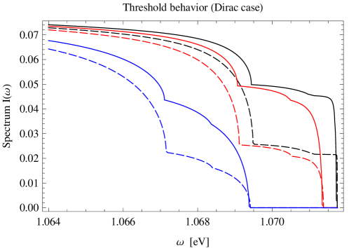
Figure 3: Photon energy spectrum from Yb ${}^{3}P_{0}\rightarrow{{}^{1}S_{0}}$ transitions in the threshold region in the cases of NH spectrum (solid lines) and IH spectrum (dashed lines) and for 3 different sets of Dirac neutrinos masses corresponding to $m_{0}=2$ meV (black lines), 20 meV (red lines) and 50 meV (blue lines).

we have: $\kappa_{33}=0$, $\kappa_{13}=\Delta m^{2}_{\rm 23}-\Delta m^{2}_{\rm 21}$, $\kappa_{23}=\Delta m^{2}_{\rm 23}$, $\kappa_{11}=4(\Delta m^{2}_{\rm 23}-\Delta m^{2}_{\rm 21})$, $\kappa_{12}=(\sqrt{\Delta m^{2}_{\rm 23}}+\sqrt{\Delta m^{2}_{\rm 23}-\Delta m^{2}_{\rm 21}})^{2}$, $\kappa_{22}=4\Delta m^{2}_{\rm 23}$. Now not only $\omega_{11}$, $\omega_{12}$ and $\omega_{22}$, but also $\omega_{13}$ and $\omega_{23}$, are very close, the corresponding differences being all $\sim\Delta m^{2}_{\rm 21}/\epsilon_{eg}$. The separation between the thresholds $\omega_{33}$ and $\omega_{13}$, and between $\omega_{23}$ and $\omega_{11}$, are considerably larger, being $\sim\Delta m^{2}_{\rm 23}/\epsilon_{eg}$. These results remain valid also in the case of QD spectrum and $\Delta m^{2}_{32}<0$.

It follows from the preceding discussion that in order to observe and determine all six threshold energies $\omega_{ij}$, the photon energy $\omega$ should be measured with a precision not worse than approximately $10^{-5}$ eV. This precision is possible in our RENP experiments since the energy resolution in the spectrum is determined by accuracy of the trigger laser frequency, which is much better than $10^{-5}$ eV.

3.2 Neutrino Observables

We will concentrate in what follows on the analysis of the dimensionless spectral function $I(\omega)$ which contains all the neutrino physics information of interest.

In Fig. 2 we show the global features of the photon energy spectrum for the Yb ${}^{3}P_{0}\rightarrow{{}^{1}S_{0}}$ transition in the case of massive Dirac neutrinos and NH and IH spectra. For $m_{0}\leq$ 20 meV, all spectra (including those corresponding to massive Majorana neutrinos which are not plotted) look degenerate owing to the horizontal and vertical axes scales used to draw the figure.

The Absolute Neutrino Mass Scale. Much richer physics information is contained in the spectrum near the thresholds $\omega_{ij}$. Figure 3 shows the Dirac neutrino spectra for three different sets of values of the neutrino masses (corresponding to the smallest mass $m_{0}=2,\;20,\;50$ meV) and for both the NO ($\Delta m^{2}_{31(32)}>0$) and IO ($\Delta m^{2}_{31(32)}<0$) neutrino mass spectra. One sees that the locations of the thresholds corresponding to the three values of $m_{0}$ (and that can be seen in the figure) differ substantially. This feature can be used to determine the absolute neutrino mass scale, including the smallest mass, as evident in differences of spectrum shapes for different masses of $m_{0}$, 2, 20, 50 meV in Fig.3. In particular, the smallest mass can be determined by locating the highest threshold ($\omega_{11}$ for NO and $\omega_{33}$ for IO). Also the location of the most prominent kink, which comes from the heavier neutrino pair emission thresholds ($\omega_{33}$ in the NO case and $\omega_{12}$ in the IO case), can independently be used to extract the smallest neutrino mass value, and thus to check consistency of two experimental methods.

If the spectrum is of the NO type, the measurement of the position of the kink will determine the value of $\omega_{33}$ and therefore of $m_{3}$. For the IO spectrum, the threshold $\omega_{12}$ is very close to the thresholds $\omega_{22}$ and $\omega_{11}$. The rates of emission of the pairs $(\nu_{2}+\nu_{2})$ and $(\nu_{1}+\nu_{1})$, however, are smaller approximately by the factors 10.0 and 12.7, respectively, than the rate of emission of $(\nu_{1}+\nu_{2})$. Thus, the kink due to the $(\nu_{1}+\nu_{2})$ emission will be the easiest to observe. The position of the kink will allow to determine $(m_{1}+m_{2})^{2}$ and thus the absolute neutrino mass scale. If the kink due to the emission of $(\nu_{2}+\nu_{2})$ or $(\nu_{1}+\nu_{1})$ will also be observed, it can be used for the individual $m_{1},m_{2}$ determination as well.

The Neutrino Mass Spectrum (or Hierarchy). Once the absolute neutrino mass scale is determined, the distinction between the NH (NO) and IH (IO) spectra can be made by measuring the ratio of rates below and above the thresholds $\omega_{33}$ and $\omega_{12}$ (or $\omega_{11}$), respectively. We note that both of these measurements can be done without knowing the absolute counting rates. For $m_{0}\ \raisebox{-1.72218pt}{\hbox to0.0pt{$\sim$\hss}}\raisebox{1.72218pt}{$<$}\ 20$ meV and NH (IH) spectrum, the ratio of the rates at $\omega$ just above the $\omega_{33}$ ($\omega_{11}$) threshold and sufficiently far below the indicated thresholds, $\tilde{R}$, is given by:

$${\rm NH}: \tilde{R}(\omega_{33};NH)\cong\frac{\sum_{i,j}|a_{ij}|^{2}-|a_{33}|^{2}}{\sum_{i,j}|a_{ij}|^{2}}\cong 0.70\,,$$ (38)

$${\rm IH}: \tilde{R}(\omega_{11};IH)\cong\frac{|a_{33}|^{2}+2\,(|a_{13}|^{2}+(|a_{23}|^{2})}{\sum_{i,j}|a_{ij}|^{2}}\cong 0.36\,.$$ (39)

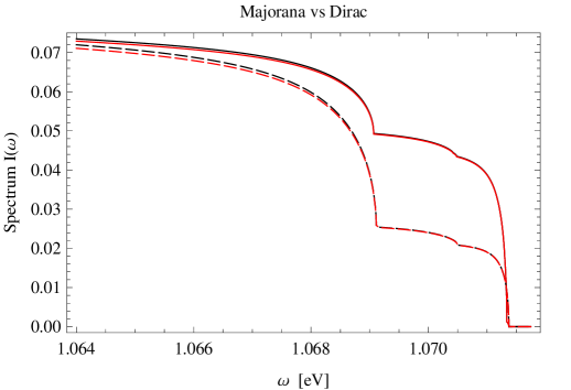
Figure 4: Spectra from Yb ${}^{3}P_{0}\rightarrow{{}^{1}S_{0}}$ transitions in the cases of Dirac neutrinos (black lines) and Majorana neutrinos (red lines) with masses corresponding to $m_{0}=20$ meV, for NH spectrum (solid lines) and IH spectrum (dashed lines).

In obtaining the result (39) in the IH case we have assumed that $\omega_{22}$ and $\omega_{12}$ are not resolved, but the kink due to the $\omega_{11}$ threshold could be observed.

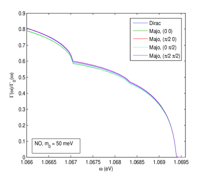
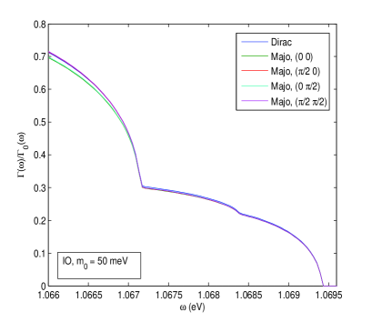
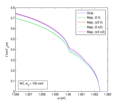
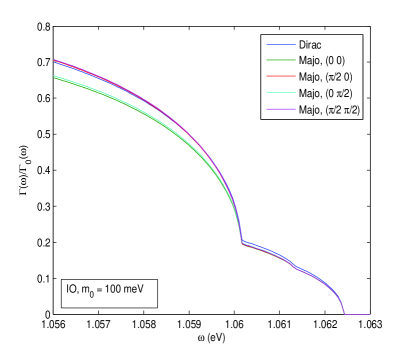
Figure 5: The ratio $R(\Gamma)\equiv\Gamma_{\gamma 2\nu}(\omega)/\Gamma_{\gamma 2\nu}(\omega;m_{i}=0)=I(\omega)/I(\omega;m_{i}=0)$ as a function of $\omega$ in the case of emission of Dirac and Majorana massive neutrinos having NO (left panels) or IO (right panels) mass spectrum corresponding to $m_{0}=50;100$ meV, for $\epsilon_{eg}=2.14$ eV and four values of the CPV phases $(\alpha,\beta-\delta)$ in the Majorana case.

The latter does not corresponds to the features shown in Fig. 3 (and in the subsequent figures of the paper), where the kink due to the $\omega_{11}$ threshold is too small to be seen and only the kink due to the $\omega_{12}$ threshold is prominent.

The Nature of Massive Neutrinos. The Majorana vs Dirac neutrino distinction is much more challenging experimentally, if not impossible, with the Yb atom. This is illustrated in Fig. 4, where the Dirac and Majorana spectra are almost degenerate for both the NH and IH cases. The figure is obtained for $m_{0}=20$ meV and the CPV phases set to zero, $(\alpha,\beta-\delta)=(0,0)$, but the conclusion is valid for other choices of the values of the phases as well.

The difference between the emission of pairs of Dirac and Majorana neutrinos can be noticeable in the case of QD spectrum with $m_{0}\sim 100$ meV and for values of the phases $\alpha\cong 0$, as is illustrated in Fig. 5, where we show the ratio $R(\Gamma)\equiv\Gamma_{\gamma 2\nu}(\omega)/\Gamma_{\gamma 2\nu}(\omega;m_{i}=0)=I(\omega)/I(\omega;m_{i}=0)$ as a function of $\omega$. As Fig. 5 indicates, the relative difference between the Dirac and Majorana spectra can reach approximately 6% at values of $\omega$ sufficiently far below the threshold energies $\omega_{ij}$. For $m_{0}=50$ meV, this difference cannot exceed 2% (Fig. 5).

A lower atomic energy scale $\epsilon_{eg}>100$ meV, which is closer in value to the largest neutrino mass, would provide more favorable conditions for determination of the nature of massive neutrinos and possibly for getting information about at least some (if not all) of the CPV phases. In view of this we now consider a

Figure 6: Majorana vs Dirac neutrino comparison in the case of X ${}^{3}P_{0}\rightarrow{{}^{1}S_{0}}$ transitions with energy difference $\epsilon_{eg}=\epsilon_{eg}({\rm Yb})/5$ for $m_{0}=2$ meV and NH (solid lines) and IH (dashed lines) spectra. The red and black lines correspond respectively to Majorana and Dirac massive neutrinos.

hypothetical atom X scaled down in energy by 1/5 from the real Yb, thus $\epsilon_{eg}\sim 0.4$ eV. There may or may not be good candidate atoms/molecules experimentally accessible, having level energy difference of order of the indicated value. Figure 6 shows comparison between spectra from X ${}^{3}P_{0}\rightarrow^{1}S_{0}$ for Majorana and Dirac neutrinos with $m_{0}=2$ meV, for both the NH and IH cases. As seen in Fig. 6, the Majorana vs Dirac difference is bigger than 5% (10%) above the heaviest pair threshold in the NH (IH) case.

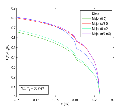
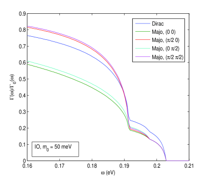
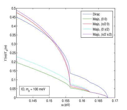
Figure 7: The same as in Fig. 5 but for $\epsilon_{eg}=0.43$ eV.

Figure 8: The dependence of $I(\omega)$ on the CPV phases $\alpha$ and $(\beta-\delta)$ in the case of NH spectrum with $m_{0}=2$ meV and for the transitions corresponding to Fig. 6. The red, solid blue and dashed blue lines are obtained for $(\alpha,\beta-\delta)=(0,0),(\pi/2,0)$ and $(0,\pi/2)$, respectively.

Figure 9: The same as in Fig. 8 for IH spectrum. The red, black solid and black dashed lines correspond to $(\alpha,\beta-\delta)=(0,0),(\pi/2,0)$ and $(0,\pi/2)$, respectively.

The difference becomes bigger for larger values of the smallest neutrino mass $m_{0}$, making the measurement easier. This is illustrated in Fig. 7, where we show again the ratio $R(\Gamma)=I(\omega)/I(\omega;m_{i}=0)$ as a function of $\omega$ in the case of Dirac and Majorana pair neutrino emission for $m_{0}=50;~{}100$ meV and NO and IO spectra. In the Majorana neutrino case, the ratio $R(\Gamma)$ is plotted for the four combinations of CP conserving values of the phases $(\alpha,\beta-\delta)=(0,0);(0,\pi/2);(\pi/2,0);(\pi/2,\pi/2)$. There is a significant difference between the Majorana neutrino emission rates corresponding to $(\alpha,\beta-\delta)=(0,0)$ and $(\pi/2,\pi/2)$. The difference between the emission rates of Dirac and Majorana neutrinos is largest for $(\alpha,\beta-\delta)=(0,0)$. For $m_{0}=50~{}(100)$ meV and $(\alpha,\beta-\delta)=(0,0)$. for instance, the rate of emission of Dirac neutrinos at $\omega$ sufficiently smaller than $\omega_{33}$ in the NO case and $\omega_{22}$ in the IO one, can be larger than the rate of Majorana neutrino emission by $\sim 20\%~{}(70\%)$. The Dirac and Majorana neutrino emission spectral rates never coincide.

In Figs. 8 and 9 we show the spectral rate dependence on the CPV phases $\alpha$ and $\beta-\delta$ for $m_{0}=2$ meV. Generally speaking, the CPV phase measurement is challenging, requiring a high statistics data acquisition. A possible exception is the case of $\alpha$ and IH spectrum, as shown in Fig. 9, where the difference between the spectral rates for $\alpha=0$ and $\alpha=\pi/2$ can reach 10%. For the NH spectrum, the analogous difference is at most a few percent; observing this case requires large statistics in actual measurements.

It follows from these results that one of the most critical atomic physics parameters for the potential of an RENP experiment to provide information on the largest number of fundamental neutrino physics observables of interest is the value of the energy difference $\epsilon_{eg}$. Values $\epsilon_{eg}\leq$0.4 eV are favorable for determining the nature of massive neutrinos, and, if neutrinos are Majorana particles, for getting information about at least some of the leptonic CPV phases, which are the most difficult neutrino related observables to probe experimentally.

4 Summary and conclusion

In the present work we investigated the sensitivity to undetermined neutrino parameters and properties (the absolute mass scale, the type of neutrino mass spectrum, the nature - Dirac or Majorana, of massive neutrinos and the CP violating phases) of the observables in macro-coherent RENP experiments. The specific case of a potential RENP experiment measuring the photon spectrum originating from ${}^{3}P_{0}\rightarrow{{}^{1}S_{0}}$ transitions in Yb atoms was considered. The relevant atomic level energy difference is $\epsilon_{eg}=2.14349$ eV. Our results show that once the RENP events are unambiguously identified experimentally, the least challenging would be the measurement of the largest neutrino mass (or the absolute neutrino mass scale). The next in the order of increasing difficulty is the determination of the neutrino mass spectrum or hierarchy (NH, IH, QD). The Majorana vs Dirac distinction and the measurement of the CPV phases are considerably more challenging, requiring high statistics data from atoms (or molecules) with lower energy difference $\epsilon_{eg}\ \raisebox{-1.72218pt}{\hbox to0.0pt{$\sim$\hss}}\raisebox{1.72218pt}{$<$}\ 0.5$ eV. Although the measurements of the indicated fundamental parameters of neutrino physics might be demanding, a single RENP experiment might provide a systematic strategy to determine almost all of these parameters, and thus can contribute to the progress in understanding the origin of neutrino masses and of the physics beyond the Standard Model possibly associated with their existence.

The present work points to the best atom/molecule candidate with level energy difference of less than O(0.5 eV) for the indicator $\epsilon_{eg}$. Besides the desirable richness of detectable observables, good candidates for realistic RENP experiments have to be searched also from the point of least complexity of target preparation. Investigations along these lines are in progress by a group including some of us.

Acknowledgements

Two of us (N.S. and M.Y.) are grateful to S. Uetake for a discussion on Yb atomic data. The research of N.S., M.T., and M.Y. was partially supported by Grant-in-Aid for Scientific Research on Innovative Areas ”Extreme quantum world opened up by atoms” (21104002) from the Ministry of Education, Culture, Sports, Science, and Technology of Japan. This work was supported in part by the INFN program on “Astroparticle Physics”, by the Italian MIUR program on “Neutrinos, Dark Matter and Dark Energy in the Era of LHC” (D.N.D. and S.T.P.) and by the World Premier International Research Center Initiative (WPI Initiative), MEXT, Japan (S.T.P.).

References

• [1] K. Nakamura and S.T. Petcov, โ€œNeutrino Mass, Mixing, and Oscillationsโ€, in J. Beringer et al. (Particle Data Group), Phys. Rev. D86 (2012) 010001.
• [2] The most recent data on the neutrino masses, mixing and neutrino oscillations were reviewed recently in several presentations at Neutrino 2012, the XXV International Conference on Neutrino Physics and Astrophysics (June 4-10, 2012, Kyoto, Japan), available at the web-site neu2012.kek.jp.
• [3] S.M. Bilenky, J. Hosek and S.T. Petcov, Phys. Lett. B94 (1980) 495.
• [4] M. Doi, T. Kotani and E. Takasugi, Phys. Lett. B102 (1981) 323; J. Schechter and J.W.F. Valle, Phys. Rev. D22 (1980) 2227.
• [5] E.ย Molinaro and S.T.ย Petcov, Eur. Phys. J. C61 (2009) 93.
• [6] L. Wolfenstein, Phys. Lett. B107 (1981) 77; S.M.ย Bilenky, N.P.ย Nedelcheva and S.T.ย Petcov, Nucl. Phys. B247 (1984) 61; B. Kayser, Phys. Rev. D30 (1984) 1023.
• [7] F.ย P.ย An et al. [Daya-Bay Collaboration], Phys. Rev. Lett. 108 (2012) 17803; D. Dwyer [for the Daya-Bay Collaboration], talk at Neutrino 2012 [2].
• [8] J.K. Ahn et al. [RENO Collaboration], Phys. Rev. Lett. 108 (2012) 191802; I. Masaki [for the Double Chooz Collaboration], talk at Neutrino 2012 [2]; T. Nakaya [for the T2K Collaboration], talk at Neutrino 2012 [2]; see also: K. Abe et al. [T2K Collaboration], Phys. Rev. Lett. 107 (2011) 041801.
• [9] G.ย L.ย Fogli et al., arXiv:1205.5254v3 [hep-ph].
• [10] M. Fukugita and T. Yanagida, Phys. Lett. B174 (1986) 45.
• [11] S. Pascoli, S.T. Petcov, and A. Riotto, Phys. Rev. D75 (2007) 083511 and Nucl. Phys. B774 (2007) 1, and references quoted therein.
• [12] G. Branco, R. Gonzalez Felipe and and F.R. Joaquim, arXiv:1111.5332 (to be published in Rev. Mod. Phys.).
• [13] M. Yoshimura, Phys. Rev. D75 (2007) 113007.
• [14] M. Yoshimura, Phys. Lett. B699 (2011) 123. The correct Majorana phase dependence in the present work is given in M. Yoshimura, A. Fukumi, N. Sasao, and T. Yamaguchi, Progr. Theor. Phys. 123 (2010) 523; see also ref. [15].
• [15] S.T. Petcov, Phys. Lett. B178 (1986) 57.
• [16] M. Yoshimura, C. Ohae, A. Fukumi, K. Nakajima, I. Nakano, H. Nanjo, and N. Sasao, Macro-coherent two photon and radiative neutrino pair emission, arXiv:805.1970[hep-ph] (2008); M. Yoshimura, Neutrino Spectroscopy using Atoms (SPAN), in Proceedings of 4th NO-VE International Workshop, edited by M. Baldo Ceolin (2008).
• [17] M. Yoshimura, N. Sasao, and M. Tanaka, Phys. Rev. A86, 013812 (2012); and arXiv:1203.5394[quan-ph] (2012).
• [18] S.M. Bilenky, S. Pascoli and S.T. Petcov, Phys. Rev. D64 (2001) 053010; S.ย Pascoli, S.T.ย Petcov and W.ย Rodejohann, Phys. Lett. B549 (2002) 177; S.ย Pascoli, S.T.ย Petcov and T.ย Schwetz, Nucl. Phys. B734 (2006) 24, and references quoted therein. see also: V. Barger et al., Phys. Lett. B540 (2002) 247.
• [19] F. Piquemal, talk at Neutrino 2012 [2].
• [20] NIST (National Institute of Standards and Technology) Atomic Spectra Database: http://www.nist.gov/pml/data/asd.cfm
• [21] For example, B.H. Bransden and C.J. Joachain, Physics of Atoms and Molecules, second edition, Prentice Hall (2003).
• [22] A. Fukumi, et al., Prog. Theor. Exp. Phys. 4 (2012) 04D002, arXiv:1211.4904 [hep-ph]; M. Yoshimura, N. Sasao, M. Tanaka, work in preparation.
• [23] S.ย M.ย Bilenky and S.ย T.ย Petcov, Rev. Mod. Phys. 59 (1987) 671.