Quasi-harmonic approximation of thermodynamic properties of ice Ih, II, and III

Abstract

Several thermodynamic properties of ice Ih, II, and III are studied by a quasi-harmonic approximation and compared to results of quantum path integral and classical simulations. This approximation allows to obtain thermodynamic information at a fraction of the computational cost of standard simulation methods, and at the same time permits studying quantum effects related to zero point vibrations of the atoms. Specifically we have studied the crystal volume, bulk modulus, kinetic energy, enthalpy and heat capacity of the three ice phases as a function of temperature and pressure. The flexible q-TIP4P/F model of water was employed for this study, although the results concerning the capability of the quasi-harmonic approximation are expected to be valid independently of the employed water model. The quasi-harmonic approximation reproduces with reasonable accuracy the results of quantum and classical simulations showing an improved agreement at low temperatures ($T$< 100 K). This agreement does not deteriorate as a function of pressure as long as it is not too close to the limit of mechanical stability of the ice phases.

I Introduction

Computer simulations of water and ice remain a very active research field after the first pioneering works more than 40 years ago.(Barker and Watts, 1969; Rahman and Stillinger, 1971) Despite the impressive progress achieved in the development of total energy computational models, simulation methods, and computer architectures, we are still far from having a standard model to simulate water at the atomistic level. In fact, water molecules are currently simulated with various degrees of sophistication. In the order of increasing complexity, one finds water models as point particles with short-range anisotropic interactions,(Moore and Valeria, 2011) as rigid molecules,(Jorgensen and Tirado-Rives, 2005; Vega and Abascal, 2011) as flexible molecules with either harmonic(Paesani et al., 2006) or anharmonic OH bonds,(Habershon et al., 2009) or as flexible polarizable molecules.(Stern and Berne, 2001; Fanourgakis and Xantheas, 2008) Accurate characterization of the electronic structure of the molecule and its chemical reactivity is only possible when ab initio methods, like density functional theory (DFT),(Benoit et al., 2002; Chen et al., 2003; Fernández-Serra and Artacho, 2004, 2006; Morrone and Car, 2008; Yoo et al., 2009) are used. Within this field, the development and application of new functionals specially designed to treat van der Waals interactions is a focus of recent interest.(Dion et al., 2004; Murray and Galli, 2012; Wang et al., 2011; Santra et al., 2011)

An additional aspect in the simulation of water phases is performing the calculation of thermodynamic properties either in a classical or a quantum limit. Evidence of the relevance of quantum effects related to nuclear motions in water phases is provided by measurements of isotope effects, that would vanish in the classical limit. As an example the melting point of ice Ih under normal conditions is shifted by 3.8 K in deuterated ice, and by 4.5 K in tritiated ice. Interestingly, the density of ice Ih shows an inverse isotope effect, i.e., D₂O ice is expanded with respect to H₂O ice,(Röttger et al., 2012, 1994) whose microscopic origin has been recently revealed.(Pamuk et al., 2012)

The path integral (PI) formulation of statistical mechanics is the most applied method to treat quantum nuclear motion in water.(Kuharski and Rossky, 1985; Mahoney and Jorgensen, 2001; Stern and Berne, 2001; Chen et al., 2003; Hernández de la Peña and Kusalik, 2004; Shiga and Shinoda, 2005; Paesani et al., 2007; Morrone and Car, 2008; Habershon et al., 2009; McBride et al., 2009; Vega et al., 2010; Ramírez and Herrero, 2010; Herrero and Ramírez, 2011a, b; Ramírez and Herrero, 2011) However, the computational cost of this method is much larger than that of its classical counterpart, and for this reason many equilibrium properties of water and ice have not been yet studied by quantum simulations. A prominent example is the complex phase diagram of ice, with fifteen different phases. To date, the simulation of relevant parts of this phase diagram has been only accessible to classical simulations using effective rigid water models.(Sanz et al., 2004; Vega et al., 2008) The computational overhead of the quantum PI simulations is caused by the need to work with multiple replicas of the system. Several approximations are available that help to reduce it. For the case of empirical point charge models of water, the ring polymer contraction scheme allows for a significant increase of computational efficiency.Markland and Manolopoulos (2008) In the case of ab initio methods the number of replicas can be reduced dramatically by means of an appropriate generalized Langevin equation.Ceriotti et al. (2011)

The quasi-harmonic approximation (QHA) has been occasionally applied to study thermodynamic properties of ice phases. Here the collective vibrations are described by a set of harmonic oscillators and thus the partition function can be expressed as an analytic function of the crystal volume and the temperature. An advantage of this approximation is that all equilibrium thermodynamic properties can be derived straightforwardly. This implies that the computational effort of the QHA is only a very small fraction of that required for a PI simulation of an ice phase, and that this fraction is independent of the chosen model potential. Further advantages of the QHA are the absence of statistical errors, as opposed to any classical or quantum simulation, and the possibility to account for finite size effects by a Brillouin zone integration of the phonon dispersion curves, rather than by increasing the size of the cell.

The QHA in combination with ab initio DFT has allowed the explanation of the inverse isotope effect in the crystal volume of ice Ih at atmospheric pressure.(Pamuk et al., 2012) Also the negative thermal expansion of ice Ih at low temperatures has been studied by the QHA,(Tanaka, 2001) as well as the elastic moduli and mechanical stability of the hydrogen ordered ice VIII.(Tse et al., 1999a) In addition, the mechanical stability of ice Ih under pressure has been studied by this approximation.(Tse et al., 1999b) One conclusion of these results is that the QHA seems to be reasonably realistic for ice phases. However, a systematic study of its potential as a predictive tool is still missing.

The purpose of this work is to check the ability of the QHA to predict thermodynamic properties of ice phases. We have analyzed three different phases (ices Ih, II, and III) in order to have a broad field of comparison. Our aim here is to compare PI results to the expectations of a much simpler QHA. We have used the point charge, flexible q-TIP4P/F model to investigate several thermodynamic properties as a function of both pressure and temperature.(Habershon et al., 2009) This model has been recently employed in PI investigations of isotope effects,(Ramírez and Herrero, 2010; Herrero and Ramírez, 2011a) proton kinetic energies,(Ramírez and Herrero, 2011) and pressure effects in water and ice Ih.(Herrero and Ramírez, 2011b) We expect that the validity of the QHA will be to a large extent independent of the employed potential model.

The layout of the manuscript is as following. Computational details of the numerical simulations and QHA of the ice phases Ih, II, and III are given in Sec. II. The phonon density of states (DOS) and the Grüneisen constants calculated with the q-TIP4P/F model are presented in Sec. III. Comparison of QHA and simulation results for various pressures ($P$) and temperatures ($T$) are presented in Sec. IV. Specifically, we study the volume ($V$), bulk modulus ($B$), kinetic energy ($K$), enthalpy ($H$), and heat capacity ($C_{p})$. Also the comparison to experimental data is presented whenever available. The paper closes with the conclusions.

II Computational procedures

In this Section we summarize some relevant computational details concerning the ice cells, the PI simulations and the QHA.

II.1 Simulation cells

Ice Ih displays proton disorder, i.e., while the oxygen atoms occupy fixed lattice positions, the water molecules display random orientations with the constraint that the resulting H-bond network must be compatible with the Bernal-Fowler ice rules.(Pauling, 1935) These rules imply that each oxygen is tetrahedrally coordinated to two H atoms by strong OH covalent bonds ($\sim$490 kJ/mol) and to two additional H atoms by weaker H-bonds ($\sim$25 kJ/mol). Ice II is an ordered phase where the molecular orientation is fully determined by the crystal symmetry. Ice III displays partial proton disorder, i.e., the occupancy of 2/3 of the crystallographic H sites deviates from 50% and it is found between 35 and 65%.(Lobban et al., 2000) Proton disordered structures with nearly zero dipole moment were generated for ice Ih and III by a simple MC algorithm designed to explore molecular orientations that obey the ice rules.(Buch et al., 1998) In line with recent computer simulations a full proton disordered structure was assumed for ice III,(Habershon and Manolopoulos, 2011; Vega et al., 2008; Cogoni et al., 2011) as this simplification seems to have only a minor effect in the phase diagram of ice.(Vega et al., 2008) The largest ice cells employed in our study contain $N=$ 288 molecules for ice Ih, and 324 molecules for ices II and III. The ice Ih cell was orthorhombic with parameters $(4\mathbf{a}_{1},3\sqrt{3}\mathbf{a}_{1},3\mathbf{a}_{3})$, with $(\mathbf{a}_{1},\mathbf{a}_{3})$ being the standard hexagonal lattice vectors of ice Ih,(Hayward and Reimers, 1997) while ice II and ice III were studied by $3\times 3\times 3$ supercells of the crystallographic cell, which belong to the rhombohedral and the tetragonal crystal systems, respectively.(Kamb et al., 1971; Lobban et al., 2000) Simulations were conducted also for smaller simulation cells to check the convergence of the results with the system size. In the following the computational conditions employed for the PIMD simulations are presented.

II.2 Path integral simulations

In the PI formulation of statistical mechanics the quantum partition function is calculated through a discretization of the integral representing the density matrix. This discretization leads to a suggestive picture: with respect to its equilibrium thermodynamic properties, the quantum system results to be isomorphic to a classical one. However, this isomorphism does not apply to the dynamic (time dependent) properties of the system. Specifically, the classical isomorph is constructed by a simple substitution of each quantum particle (here, atomic H and O nucleus in the water molecule) by a ring polymer of $L$ classical particles (beads), connected by harmonic springs with a temperature- and mass-dependent force constant. Details of this practical simulation method can be found elsewhere.(Feynman, 1972; Gillan, 1988; Ceperley, 1995; Chakravarty, 1997) Equilibrium properties in the classical isomorph can be derived by a classical molecular dynamics (MD) algorithm, that has the advantage against a Monte Carlo method of being more easily parallelizable, an important fact for efficient use of modern computer architectures. Effective reversible integrator algorithms to perform PIMD simulations have been described in Refs. Martyna et al., 1999; Tuckerman, 2002; Tuckerman and Hughes, 1998; Tuckerman et al., 1993. Ref. Martyna et al., 1996 introduces useful methods to treat full cell fluctuations and multiple time step integration. All simulations were done using originally developed software and parallelization was implemented by the MPI library.(Pacheco, 1997) The potential energy of each replica of the system is calculated in parallel by a different processor. Other interesting optimization schemes, not used in this work, are based on ring polymer contraction techniques.Markland and Manolopoulos (2008)

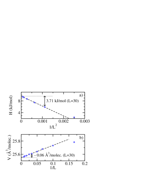
Figure 1: Results for the convergence of the enthalpy (a) and volume (b) of ice II with the number of beads ($L$) employed in the PIMD simulations. The constant shifts that correct the finite $L$ results derived with the condition $LT=$ 6000 K are explicitly shown. The simulations were performed at $T=$200 K and $P=$1 atm.

PIMD simulations in the isothermal-isobaric $NPT$ ensemble ($N$ being the number of water molecules) were conducted for ice Ih, II, and III at temperatures up to 300 K and pressures between -1 and 2 GPa. We have employed the point-charge, flexible q-TIP4P/F model, that was originally parameterized to provide the correct liquid structure, diffusion coefficient, and infrared absorption frequencies in quantum simulations.(Habershon et al., 2009) Periodic boundary conditions were applied to the simulation cell and the Ewald method was employed to calculate the long range electrostatic potential and atomic forces. Expected averages were derived in runs of $10^{6}$ MD steps (MDS) using a time step of $\Delta t=0.2$ fs. The system equilibration was conducted in runs of $10^{5}$ MDS. To have a nearly constant precision as a function of temperature, the number of beads $L$ was set as the integer number closest to fulfill the relation $LT=6000$ K, i.e., at 200 K the number of beads was $L=30$. The classical limit is easily achieved by setting $L$=1 in the PIMD algorithm. The largest error associated to the finite number of beads is caused by the highest energy vibrations, i.e., the intramolecular OH stretching modes. These modes remain essentially in their ground state as their energy quantum ($\hbar\omega_{OH}$) is several times larger ($\sim 16$) than the thermal energy ($k_{B}T$) at the highest studied temperature. Thus we expect this error to be a nearly $T$ (and $P$) independent shift. The shift has been estimated for the quantities of interest (volume, enthalpy, and kinetic energy) by a series of $NPT$ simulations of the three ice phases using different numbers of beads at $T$= 200 K and $P$= 1 atm. The $L\rightarrow\infty$ limit was extrapolated from the best linear fit in either the variable $1/L^{2}$ or $1/L$. In Fig. 1 the result of this extrapolation is represented for both the enthalpy and volume of ice II. The constant shifts that correct the thermal averages derived with the relation $LT=6000$ K are 3.71 kJ/mol for the enthalpy and 1.89 kJ/mol for the kinetic energy. The corresponding correction shift for the volume amounts to -0.03 $\textrm{\AA}^{3}$/molecule for ice Ih and III, and -0.06 $\textrm{\AA}^{3}$/molecule for ice II. Additional computational conditions in the simulations were identical to those reported in Ref. Ramírez and Herrero, 2010.

II.3 Quasi-harmonic approximation

II.3.1 Basic equations

The quasiharmonic approximation employed here is based on the following three assumptions:

$a)$ the simulation cell, defined by the vectors ($\mathbf{a}_{1},\mathbf{a}_{2},\mathbf{a}_{3})$, is considered to scale isotropically with the crystal volume, $V$, as

$$\mathbf{a}_{i}(V)=(V/V_{ref})^{1/3}\mathbf{a}_{i,ref}\;,i=1,2,3\;,.$$ (1)

$V_{ref}$ is the volume of the reference cell ($\mathbf{a}_{1,ref},\mathbf{a}_{2,ref},\mathbf{a}_{3,ref})$ that minimizes the potential energy at a certain chosen pressure, $P_{ref}$, where the ice phase is mechanically stable.

$b)$ the lattice vibrations are described by harmonic oscillators of wavenumber $\omega_{k}$, with $k$ combining the phonon branch index and the wave vector within the Brillouin zone.

$c)$ the wavenumbers $\omega_{k}$ depend on the volume of the crystal, which may change with temperature and pressure. However, for a given volume the wavenumbers $\omega_{k}$ are constants (independent of $T$ and $P$) as in a harmonic approximation.

With these assumptions, the Helmholtz free energy of the ice cell with $N$ molecules in a volume $V$ and at temperature $T$ is given by

$$F(V,T)=U_{S}(V)+F_{v}(V,T)-TS_{H}\;,$$ (2)

where $U_{S}(V)$ is the static zero-temperature classical energy, i.e., the minimum of the potential energy when the volume of the ice cell is $V$. The entropy $S_{H}$ is related to the disorder of hydrogen, it vanishes for ice ordered phases as ice II. $S_{H}$ was estimated by Pauling for fully disorder phases using simple counting schemes of allowed water orientations (Pauling, 1935)

$$S_{H}=Nk_{B}\ln\frac{3}{2}\;.$$ (3)

$F_{v}(V,T)$ is the vibrational contribution to $F$,

$$F_{v}(V,T)=\sum_{k}\left(\frac{\hbar\omega_{k}}{2}+\frac{1}{\beta}\ln\left[1-\exp\left(-\beta\hbar\omega_{k}\right)\right]\right)\;.$$ (4)

Here $\beta$ is the inverse temperature: $1/k_{B}T.$ This expression for $F_{v}$ is valid for quantum harmonic oscillators. If one is interested in the classical limit of the QHA the vibrational contribution changes to

$$F_{v,cla}(V,T)=\sum_{k}\frac{1}{\beta}\ln\left(\beta\hbar\omega_{k}\right)\;.$$ (5)

The terms $U_{S}(V)$ and $S_{H}$ remain the same for either a quantum or classical limit. The calculation of those thermodynamic properties derived from the partition function (as the Gibbs free energy, enthalpy, internal energy, kinetic energy, state equation, thermal expansion, bulk modulus, heat capacity, etc.) can be easily performed with the help of Eq. (2). For example, the Gibbs free energy, $G(T,P),$ can be derived by seeking for the volume, $V_{min}$, that minimizes the function $F(V,T)+PV$, as

$$G(P,T)=F(V_{min},T)+PV_{min}\;.$$ (6)

II.3.2 Direct implementation

The direct implementation of the QHA implies the following steps:

$a)$ determination of the ice reference cell by an energy minimization where both water molecules and cell parameters are simultaneously optimized. Both the shape of the reference cell and its volume $V_{ref}$ are obtained in this step.

$b)$ a set of cell volumes $\left\{V_{i}\right\}$ of interest is selected.

$c)$ given a cell volume $V_{i}$, the simulation cell is derived by the scaling of the reference cell as shown by Eq. (1). The water molecules are then relaxed to their minimum potential energy and the crystal phonons are calculated and tabulated. This tabulation allows us the calculation of $F(V_{i},T)$ for the set of volumes $\left\{V_{i}\right\}$ by means of Eq (2).

$d)$ for the purpose of finding the minimum of $F(V_{i},T)$ as a function of $V$ (or alternatively, the minimum of $G=F+PV$), it is convenient to perform a polynomial fit of $F(V_{i},T)$ and then look for the minimum of the fitted function.

This implementation requires, for each of the studied volumes $V_{i}$, a crystal structure minimization and the calculation of the corresponding crystal phonons. Typically we have selected a set of 50 different $V_{i}$ for each ice phase and chosen a 5th degree polynomial as fitting function to find the minimum of $F(V,T)$ as a function of $V$. Using an empirical potential this implementation is straightforward and does require a little amount of computer time even for simulation cells containing several hundreds of water molecules.

The crystal phonon calculation has been performed by the small-displacement, or frozen phonon method.(Kresse et al., 1995; Alfè et al., 2001) The basic principle is to compute the force constants between atom pairs numerically deriving the (analytic) forces. Atoms are displaced a small, but finite, amount from their perfect-lattice positions, and all the atomic forces generated by this displacement are calculated. Given that the displacement is small, the force constant describes the proportionality between displacements and forces. The atomic displacement employed in this work is $\delta x=10^{-6}$ Å along each cartesian direction. Although we have used a flexible water model, the method can be also applied to rigid water models by allowing molecular displacements associated with small translations and rotations of the rigid units. See Ref. [Venkataraman and Sahni, 1970] for a full account of the calculation of the external phonon modes associated to rigid molecules.

The QHA results have been derived by a $\Gamma$ ($\mathbf{k}=0$) sampling of the Brillouin zone of the ice simulation cell. Although this is an adequate approximation, given the large size of the employed cells, its main justification is that we are interested in the comparison to PIMD simulations. Note that the application of periodic boundary conditions in the simulation implies that all atomic images move in phase, and this corresponds exactly to the spatial symmetry of the $\mathbf{k}=0$ phonons.

II.3.3 A simpler implementation

For calculations based on non-empirical potentials of water, e.g., in ab initio DFT theory, it may be computationally convenient to reduce the number of energy minimizations and phonon calculations by using the phonon-dependent Grüneisen parameters defined as(Ashcroft and Mermin, 1976)

$$\gamma_{k}=-\left(\frac{\partial\ln\omega_{k}}{\partial\ln V}\;\right)_{V_{ref}}.$$ (7)

This equation can be integrated assuming that $\gamma_{k}$ is a volume independent constant to obtain the volume dependence of $\omega_{k}$ as

$$\omega_{k}(V)\approx\omega_{k}(V_{ref})\times\left(\frac{V}{V_{ref}}\right)^{-\gamma_{k}}\;.$$ (8)

A linear expansion of the previous relation, i.e., taking the derivative $(\partial\omega_{k}/\partial V)$ as a constant independent of $V$, leads to the alternative expression

$$\omega_{k}(V)\approx\omega_{k}(V_{ref})\times\left(1-\frac{V-V_{ref}}{V_{ref}}\gamma_{k}\right)\;.$$ (9)

The last two relations allow us to calculate the function $F_{v}(V,T)$ in Eq. (4) from a tabulation of the values $(\omega_{k},\gamma_{k})$ obtained for the reference cell. We have compared the direct implementation of the QHA (see Sect. II.3.2) with the simpler implementation of Eqs. (8) and (9) by calculating the function $V(T)$ at $P=0$. We find that Eq. (9) works slightly better than Eq. (8) for ice Ih, while for ice II and III the opposite behavior was observed. A recent QHA study of the thermal expansion of ice Ih using DFT was based on Eq. (9).(Pamuk et al., 2012) Note that the numerical calculation of the Grüneisen constants requires at least two energy minimizations and phonon calculations (at $V_{ref}$ and at an additional volume in the proximity of $V_{ref}$). Therefore the computational cost of this simpler implementation is reduced by about a factor of 25 in comparison to the previous direct implementation of the QHA. In the next Section the direct implementation of the QHA is applied to the study of ice phases.

Table 1: Volume, potential energy, and simulation cell parameters of the reference cells of ice Ih, II, and III obtained by energy minimizations with the q-TIP4P/F model at $P_{ref}=0.$ The direct implementation of the QHA implies a phonon calculation at 50 different volumes uniformly distributed in the interval [$V_{min},$$V_{max}$].

	Ih		II		III
$N$ (molecules/cell)	288		324		324
$V_{ref}$ (ų/molec.)	30.	96	24.	14	24.	99
$U_{S,ref}$ (kJ/mol)	-61.	98	-60.	84	-60.	86
$\triangle U_{S,ref}$ (kJ/mol)	-1.	15	0		-0.	02
$a_{1,ref}$ ($\textrm{\AA})$	17.	78	22.	98	19.	68
$a_{2,ref}$ ($\textrm{\AA})$	23.	09	22.	98	19.	77
$a_{3,ref}$ ($\textrm{\AA})$	21.	76	22.	98	20.	80
$\alpha$ (0)	90.	0	113.	2	89.	9
$\beta$ (0)	90.	0	113.	2	89.	9
$\gamma$ (0)	90.	0	113.	2	89.	8
$V_{min}$(ų/molec.)	29.	47	21.	75	22.	48
$V_{max}$ (ų/molec.)	35.	05	27.	31	28.	22

III Q-tip4p/f ice phonons

Reference cells for the QHA have been derived at $P_{ref}$=0 for the three ice phases by energy minimizations implying optimization of both atomic positions and simulation cell. Optimized simulation cells as well as the corresponding volumes ($V_{ref})$ and potential energies ($U_{S,ref})$ are summarized in Tab. 1. The direct implementation of the QHA involved the calculation of the vibrational modes for 50 different volumes uniformly distributed in the interval [$V_{min},$$V_{max}$] (see Tab. 1). Note that the largest volume per molecule corresponds to ice Ih (28% and 24 % larger than those of ices II and III, respectively). By setting the potential energy of ice II as the zero of the energy scale, the structure of ice Ih results more stable by $\triangle U_{S,ref}$=-1.15 kJ/mol, a value in good agreement to that of -1.17 kJ/mol reported in Ref. Habershon and Manolopoulos, 2011. However, for ice III we find $\triangle U_{S,ref}=$ -0.02 kJ/mol, significantly different from the previously reported result of -0.1 kJ/mol.(Habershon and Manolopoulos, 2011) We have checked that this difference is a consequence of the disorder of hydrogen in ice III. Support for this is given by the equilibrium potential energies $U_{S,ref}$ of a series of five randomly generated ice III structures. These energies scatter in an energy window of 0.2 kJ/mol, a value more than two times larger than the energy difference between our results and the one Ref. Habershon and Manolopoulos, 2011. Interestingly this effect is much smaller in disordered ice Ih, where the energy fluctuations computed for five randomly generated structures are reduced by more than an order of magnitude to about 0.01 kJ/mol.

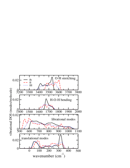
Figure 2: Vibrational density of states obtained for the reference cells of ice Ih, II, and III with the q-TIP4P/F water model. The harmonic modes correspond to a $\Gamma$ sampling of the Brillouin zone and each mode was plotted as a normalized Gaussian with a width of 10 cm^-1.

The vibrational DOS calculated with the q-TIP4P/F model for the reference cells of the three ice phases are shown in Fig.2. The wavenumbers of the vibrational modes are separated into four groups comprising 3$N$ translational, 3$N$ librational, $N$ bending, and 2$N$ stretching modes. Translational and librational modes are related to the intermolecular interactions and can be differentiated not only by their respective frequency windows but also by their effective masses. The translational modes display a “heavy” molecular mass while the librational modes display a “light” hydrogen mass, a fact that can be experimentally observed by the frequency shifts found after isotopic substitution of either O or H atoms. Within a harmonic approximation this shift scales as the squared root of the effective mass. The intramolecular modes (bending and stretchings) display also a “light” hydrogen mass. It is interesting to observe the anticorrelation between librational and stretching modes in the ice phases: the lower the frequency of librational modes, the higher the frequency of the stretchings modes.(Libowitzky, 1999; Bratos et al., 2009) The calculated Grüneisen constant for ice Ih and III are displayed in Fig. 3.

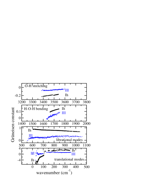
Figure 3: Grüneisen constants of ice Ih and III calculated for the q-TIP4P/F model. Results for ice II lie in-between ice Ih and III and are not shown for clarity.

A fingerprint of the vibrational structure of the ice phases is presented in Tab. 2, that summarizes the result of averaging the complete set of $9N$ wavenumbers calculated for the ice reference cell into 9 groups of $N$ modes taken from a list ordered by increasing wavenumber. The resulting average frequencies and Grüneisen constants reveal significant differences between the ice phases. The negative Grüneisen constant associated to the $N$ translational modes of lowest energy is the origin of the negative thermal expansion experimentally found in ice Ih at low temperature.(Röttger et al., 1994) For ice II the averaged Grüneisen constant of these modes is also negative but much smaller in absolute value, while for ice III is positive. Negative Grüneisen parameters are also found for the $2N$ stretching vibrations with absolute values in the order Ih>II>III. We note that the Grüneisen constants of the stretching vibrations in the q-TIP4P/F model are a factor of two smaller than those obtained in the ab initio DFT study of ice Ih.(Pamuk et al., 2012) These larger DFT absolute values are crucial to correctly describe the experimental inverse isotope effect found in the crystal volume of normal and deuterated ice Ih, (Pamuk et al., 2012) an effect that is not reproduced by the q-TIP4P/F model.(Herrero and Ramírez, 2011a)

Table 2: Average of the 9$N$ harmonic modes obtained for the reference cells of the ice phases with the q-TIP4P/F model into groups of $N$ modes. The average wavenumbers and Grüneisen constants are a fingerprint of the vibrational structure of each ice phase.

		$\left\langle\omega_{k}\right\rangle$ (cm-1)				$\left\langle\gamma_{k}\right\rangle$
modes	Ih	II	III	Ih		II		III
$N$ translational	60	76	63	-3.	32	-0.	14	0.	14
$N$ translational	223	194	209	2.	47	2.	44	1.	14
$N$ translational	323	302	319	2.	74	2.	67	1.	10
$N$ librational	650	574	613	0.	86	0.	78	0.	20
$N$ librational	758	673	726	0.	81	0.	76	0.	24
$N$ librational	904	859	907	0.	75	0.	64	0.	32
$N$ bending	1691	1678	1684	0.	11	0.	10	0.	03
$N$ stretching	3439	3506	3453	-0.	20	-0.	15	-0.	07
$N$ stretching	3522	3587	3549	-0.	18	-0.	13	-0.	05

IV QHA Results

In this Section we evaluate the performance of the QHA in the description of ice Ih, II, and III by comparing it to PIMD simulation results. Our study is focused on the temperature and pressure dependence of several ice properties as crystal volume, bulk modulus, kinetic energy, enthalpy, and heat capacity. Both quantum and classical limits have been studied, and compared to experimental results whenever they are available.

IV.1 Thermal expansion

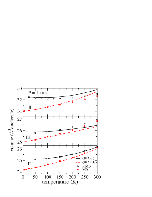
Figure 4: Thermal expansion of ice Ih, II, and III at atmospheric pressure calculated with the q-TIP4P/F water model. The QHA results (lines) are compared to PIMD and MD simulations (symbols). Both quantum (q) and classical (cla) limits are shown. Error bars of the simulation results are less than the symbol size.

The temperature dependence of the crystal volume at atmospheric pressure derived from the QHA is compared to PIMD results in Fig. 4. Both quantum and classical limits are shown for the three ice phases. The QHA reproduces the simulation results rather accurately up to temperatures of 100 K. At higher temperatures anharmonic effects not included in the QHA cause deviations of different sign in the ice Ih and III curves, while for ice II the agreement with the PIMD data is good up to the highest studied temperature. The QHA estimation of the zero point expansion (i.e. the volume increase with respect to the classical limit at $T$=0) of the q-TIP4P/F model amounts to 4% for ice Ih and II, and to 3.6% for ice III.

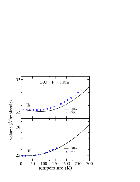
Figure 5: Temperature dependence of the volume of D₂O ice Ih and II at atmospheric pressure. The QHA results (lines) are compared to the experimental data (circles) of ice Ih (Ref. Röttger et al., 1994) and II (Ref. Fortes et al., 2005).

The comparison of the QHA result to available experimental data(Röttger et al., 1994; Fortes et al., 2005) at atmospheric pressure is presented in Fig. 5 for deuterated ices Ih and II. The overall agreement is good, in particular for ice II. At low temperatures there appears a negative thermal expansion in both experimental and q-TIP4P/F results of ice Ih. However, for ice II this effect is not appreciable at the scale of the figure. This behavior of ice Ih and ice II can be rationalized by the differences in the average Grüneisen constant of the $N$ translational modes of lowest frequency (see Tab. 2 for values calculated for the H₂O ices). The negative thermal expansion of ice Ih is a stringent test of the water model. An interesting comparison of several effective potentials reveals that the negative thermal expansivity of ice Ih is succesfully reproduced by the TIP4P model. However this effect is absent in the TIP5P potential and only slightly visible with the ST2 model.Koyama et al. (2004)

IV.2 State equation at 100 K

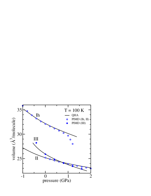
Figure 6: Equation of state of ice Ih, II, and III at 100 K. QHA results (lines) are compared to PIMD simulations (symbols). All results were derived with the q-TIP4P/F water model. Error bars of the simulation results are less than the symbol size.

The pressure dependence of the volume of the ice phases is presented in Fig. 6 at temperature of 100 K. The QHA shows good agreement with PIMD results. The sudden drop of the PIMD data of ice Ih at high pressures is due to the proximity of the spinodal pressure at about 1.2 GPa where ice Ih becomes mechanically unstable and collapses into a high-density amorphous (HDA) ice in simulations with the q-TIP4P/F model.(Herrero and Ramírez, 2011b) Interestingly this limit of mechanical stability of ice Ih is also captured by the QHA. By increasing the hydrostatic pressure the QHA predicts a compressed ice Ih volume characterized by the appearance of soft phonons that reach a vanishing vibrational frequency at a pressure slightly below 1.4 GPa.

The best overall agreement between PIMD and QHA results is found for H ordered ice II. In the case of ice III a significant deviation is found at negative pressures of about -0.5 GPa, but for positive pressures the QHA provides accurate results.

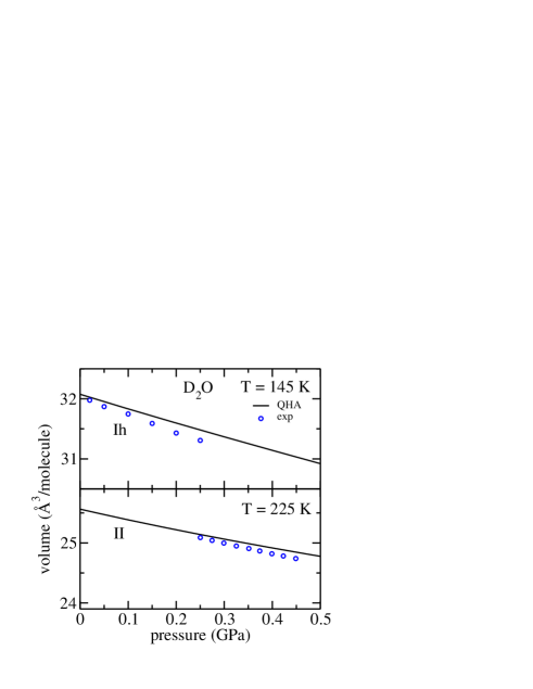
Figure 7: Equation of state of D₂O ice at 145 K (ice Ih) and 225 K (ice II). The QHA (lines) is compared to experimental data (circles) of ice Ih (Ref. Strässle et al., 2005) and II (Ref. Fortes et al., 2005).

The experimental results for D₂O ice at 145 K (ice Ih)(Strässle et al., 2005) and 225 K (ice II)(Fortes et al., 2005) are compared to the QHA expectation in Fig. 7. The experimental data show the pressure window where each phase is stable at the studied temperature. Note the large volume difference between the two ice phases. The QHA predicts reasonable results for both phases specially in the low pressure region of each phase. The main difference to the experimental data is seen by the slope of the $V(P)$ curve, i.e., the QHA using the q-TIP4P/F model overestimates the hardness of both ices Ih and II (it predicts a larger bulk modulus).

IV.3 Bulk modulus

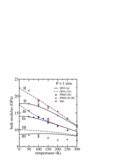
Figure 8: Temperature dependence of the bulk modulus of ice Ih, II, and III derived with the q-TIP4P/F mode at atmospheric pressure. The QHA results in the quantum and classical limits (lines) are compared to PIMD and classical MD simulations, respectively (symbols). Typical error bars in the simulation results are shown at 100 K (ices II and III) and 150 K (ice Ih).

The temperature dependence of the bulk modulus of the three studied ice phases is presented in Fig. 8. The bulk modulus in the MD simulations is calculated from the fluctuation formula of the cell volume in the $NPT$ ensemble.(Herrero and Ramírez, 2011b) At any given temperature the order of increasing bulk modulus (less compressibility) is: ice III < Ih < II. The QHA of ice II provides results in excellent agreement with quantum PIMD and classical MD simulations. Also for ice Ih we find that the QHA provides good results. A worse agreement is found for ice III where the QHA predicts a bulk modulus somewhat larger than the PIMD results. Classical and quantum results above 100 K are not very different from each other specially for ice III and Ih. The statistical error of the bulk modulus in the MD simulations is large. The classical MD results for ice III have not been represented as its statistical error was of the order of its difference to the PIMD data.

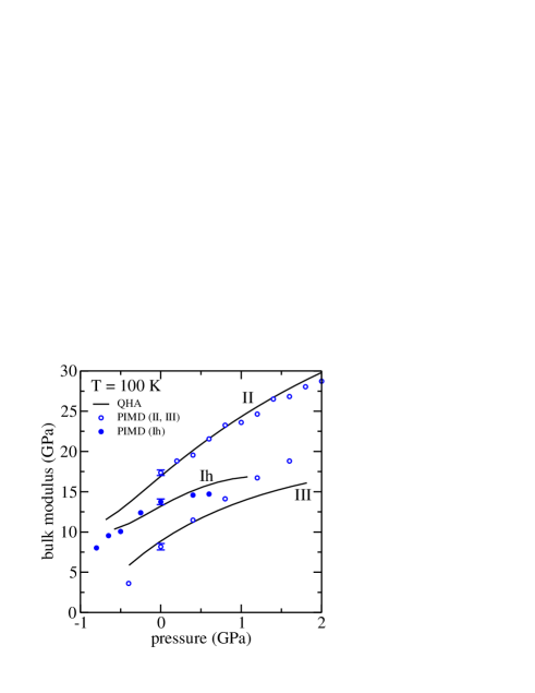
Figure 9: Pressure dependence of the bulk modulus of ice Ih, II, and III calculated with the q-TIP4P/F model at 100 K. QHA results (lines) are compared to PIMD simulations (symbols). The estimated error bars of the simulation results are shown at $P=$ 0.

The pressure dependence of the bulk modulus of ice Ih, II, and III calculated with the QHA is compared in Fig. 9 with the results of PIMD simulations at 100 K. The increase with pressure of the bulk modulus predicted by the QHA agrees rather accurately with the PIMD data in the case of ice II and ice Ih. For ice III we find again a worse agreement between QHA and MD simulation results. Nevertheless, the largest deviations between both sets of data are found either at negative pressures or at positive ones larger than 0.35 GPa. This value is the coexistence pressure experimentally found at 100 K between ice III and the higher pressure phase ice V.(Dunaeva et al., 2010)

IV.4 Kinetic energy

Figure 10: Kinetic energy of ice Ih, II, and III at atmospheric pressure calculated with the q-TIP4P/F water model. The QHA results (full lines) are compared to PIMD (symbols). For ice Ih both quantum (q) and classical (cla) limits are shown. Error bars of the simulation results are smaller than the symbol size.

The internal energy is given by the sum of potential and kinetic energy contributions. Within the QHA both energy terms must be identical as a consequence of the virial theorem. A comparison of the QHA and PIMD estimations of the kinetic energy, $K$, at atmospheric pressure is presented in Fig. 10 as a function of temperature. For ice Ih we compare also the quantum results to the classical limit (broken line), that amounts to $k_{B}T/2$ per degree of freedom (equipartition principle). The QHA estimation of the zero point kinetic energy of ice Ih is 34.4 kJ/mol. Nearly the same value is obtained for ice III, while for ice II we get a reduced zero-point energy energy of 34.0 kJ/mol. This difference implies that ice II is stabilized with respect to ice Ih and ice III due to its lower zero point energy. The comparison of QHA and PIMD data shows that the QHA overestimates the value of $K$ by about 0.8 kJ/mol in the three ice phases and that this shift is nearly temperature independent.

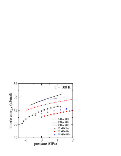
Figure 11: Kinetic energy of the studied ice phases as a function of the pressure at 100 K. QHA results (lines) are compared to PIMD simulations (symbols). Error bars of the simulation results are in the order of the the symbol size.

The pressure dependence of the kinetic energy at 100 K is displayed in Fig. 11. Here we also find that QHA results are shifted with respect to the PIMD data. The shift remains nearly constant with the pressure, except for the case of ice Ih at the highest simulated pressures, where larger deviations are originated from the proximity to the limits of the mechanical stability of this ice phase.

IV.5 Enthalpy

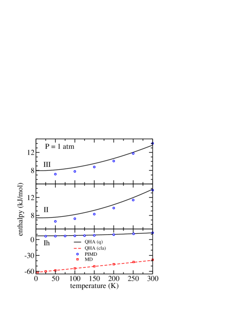
Figure 12: Enthalpy of ice Ih, II, and III at atmospheric pressure calculated with the q-TIP4P/F water model. The QHA results (lines) are compared to PIMD and MD simulations (symbols). For ice Ih both quantum and classical limits are shown. Error bars of the simulation results are less than the symbol size.

At atmospheric pressure the enthalpy of ice is nearly identical to its internal energy as the term $PV$ results to be vanishingly small. The enthalpy, $H$, of the three ice phases at atmospheric pressure is presented in Fig. 12 as a function of temperature. For ice Ih we have compared both the classical and quantum limits of the QHA to the corresponding simulation results. At the scale of the figure the agreement is very good. The QHA zero-point energy of ice Ih is 68.9 kJ/mol. The QHA systematically overestimates the enthalpy of the three ice phases at low temperatures. In the case of ice Ih we find that at 50 K the QHA result is 0.7 kJ/mol larger than the PIMD result, while for ice II and III we obtain a larger deviation of about 0.9 kJ/mol. Both QHA and PIMD results show that at 50 K the enthalpy of the ice phases increases in the order Ih$<$II$<$III. With respect to the enthalpy of ice II, the relative values found for ice Ih and III at 50 K are -0.3 and 0.5 kJ/mol (PIMD) and -0.4 and 0.5 kJ/mol (QHA), respectively. Interestingly at higher temperature the agreement between the PIMD and QHA data becomes better as a consequence of an error compensation between kinetic and potential energy terms. Thus the error of the QHA enthalpy estimation is lower than that found for the kinetic energy in the previous Subsec. IV.4.

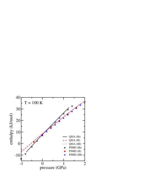
Figure 13: Enthalpy of the studied ice phases as a function of the pressure at 100 K. QHA results (lines) are compared to PIMD simulations (symbols). Error bars of the simulation results are smaller than the symbol size.

The pressure dependence of the enthalpy at 100 K is represented in Fig. 13. The term $PV$ plays here an important role. We have already seen in Fig. 12 that at 100 K and atmospheric pressure the QHA overestimates the reference enthalpy of PIMD simulations. This behavior results nearly independent of the external pressure. In Fig. 13 the QHA result for the three ice phases lies systematically slightly above the corresponding simulation results, but the overall agreement can be considered as satisfactory in the whole studied pressure range.

IV.6 Heat capacity

The heat capacity at constant pressure is defined as

$$C_{p}=\left(\frac{\partial H}{\partial T}\right)_{P}\quad.$$ (10)

The PIMD estimation of $C_{p}$ of ice Ih at atmospheric pressure has been obtained from a numerical fit of the $H(T)$ curve shown in Fig. 12. The temperature derivative was calculated from a 4th degree polynomial fit of $H(T)$ in the interval 80-190 K. The result is plotted as filled circles in Fig. 14. For comparison the experimental $C_{p}$ data of ice Ih of Refs. Giauque and Stout, 1936; Smith et al., 2007 have been plotted as open circles and squares, respectively. We find good agreement between the PIMD results and the experimental data. The figure also includes lines showing the $C_{p}$ values derived from the QHA of ice Ih, II, and III, with an inset that highlights their low temperature behavior. Note that the QHA underestimates the PIMD data of ice Ih at temperatures above 100 K. However, the QHA result appears close to the simulation at 80 K. At low temperatures (below 40 K, see the inset of Fig. 14) the QHA for ice Ih shows an excellent agreement to the experimental data. We expect that such a good agreement will occur also in PIMD simulations. However, the computational cost of these PIMD simulations increases as $1/T$, along with the increase in the number of beads, so that a reliable simulation of $C_{p}$ below 40 K becomes computationally too expensive. Therefore the QHA seems to be a practical alternative to PIMD simulations in the study of the low temperature heat capacity of ices.

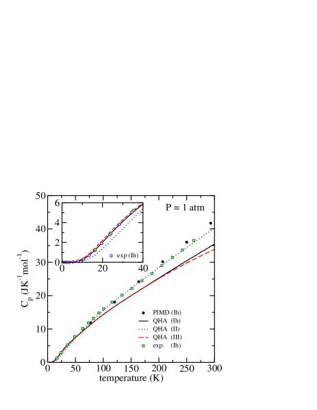
Figure 14: Heat capacity of ice Ih, II, and III at atmospheric pressure. Lines are results derived by the QHA. Filled circles correspond to PIMD simulations of ice Ih. Experimental data for ice Ih are shown by open circles (Ref. Smith et al., 2007) and open squares (Ref. Giauque and Stout, 1936). The inset emphasizes the low temperature limit.

The heat capacities of the three ice phases are significantly different in the studied temperature range. In particular, below 50 K ice II displays the lowest heat capacity at the studied pressure, while the opposite behavior is observed above this temperature.

It has been previously stressed that the pressure dependence of $C_{p}$ in ice Ih has not been studied experimentally. Thus the empirical equation of state of Feistel and Wagner has been applied to extrapolate the temperature dependence of $C_{p}$ at pressures up to 0.2 GPa.(Feistel and Wagner, 2006) In particular the temperature dependence of the relative heat capacity

$$\Delta C_{p}=C_{p}(P)-C_{p}(P_{ref}=0)$$ (11)

derived at $P$=0.2 GPa with this empirical equation of state is represented by full symbols in Fig. 15. This extrapolation of $\Delta C_{p}$ is characterized by having a rather small slope at low and at high temperatures. The same qualitative behavior is found for lower pressures.(Feistel and Wagner, 2006) On the contrary, the QHA predicts a different overall behavior, with a maximum of $\Delta C_{p}$ at low temperatures ($\sim 25$ K) and a conspicuous negative slope at high temperatures. We believe that the QHA provides a more realistic estimation of $\Delta C_{p}$ than that obtained by extrapolation of the empirical equation of state. Our main argument is that the QHA represents a realistic physical model of the ice phase.

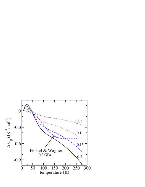
Figure 15: Relative heat capacity, $C_{p}(P)-C_{p}(P_{ref}=0)$, of ice Ih as a function of temperature. The QHA results are shown by lines labeled by the calculation pressure (in GPa). The curve with symbols was derived by the empirical state equation of Ref. Feistel and Wagner, 2006 at a pressure of 0.2 GPa.

V Conclusions

In this work we have undertaken a systematic study of the capability of the QHA to reproduce several thermodynamic properties of ice Ih, II, and III as a function of both pressure and temperature. The studied pressure range goes from -1 to 2 GPa, while the temperatures were studied up to 300 K. Thus the region in the $P-T$ plane where the QHA has been checked is much larger than the area where the studied ice phases are found to be thermodynamically stable. Therefore an important consideration of the present study is its generality, in the sense that it is not limited to a small number of state points.

The validity of the QHA is restricted by the presence of anharmonic effects not included in the approximation. Thus a direct check of the QHA is the comparison to numerical simulations that fully consider the anharmonicity of the interatomic interactions. We have employed the empirical q-TIP4P/F model for this comparison. Our expectation that the validity of the QHA is largely independent of the employed water model is based on the assumption that the anharmonicity of the q-TIP4P/F potential is reasonably realistic in view of the large body of experimental data reproduced by this model.Habershon et al. (2009); Ramírez and Herrero (2010); Herrero and Ramírez (2011b)

The comparison of the QHA to the PIMD simulations shows a remarkable overall agreement for the three ice phases. The best agreement has been found for ice II, which is an ordered phase of ice. Both crystal volume and enthalpy have been shown to be reasonably reproduced by the QHA. This fact let us expect that the QHA could be appropriate to study phase coexistence of ice phases as the slopes of phase coexistence lines are a function of the differences in volume and enthalpy of the corresponding ice phases (Clausius-Clapeyron relation). The QHA is also particularly appropriate to study the low temperature limit of certain thermodynamic properties as the heat capacity, bulk modulus and internal energies. The computational cost of PI simulations increases as $1/T$, so that the simulation of low temperature limits can be prohibitively expensive by this approach. Further advantages offered by the QHA are the lack of statistical errors and the easier checking and correction of finite size errors. These advantages apply not only compared to PI simulations, but even compared to classical MD.

The experimental heat capacity of ice Ih at low temperatures ($T<$40K) is reproduced with remarkable accuracy with the QHA at atmospheric pressure. Our results lead us to expect that this good agreement should not deteriorate at higher pressures. We have shown that the temperature dependence of heat capacities at finite pressures predicted by the QHA differs in important aspects from a previous estimation based on the extrapolation of the Feistel-Wagner equation of state for ice Ih.Feistel and Wagner, 2006 Although we have not found experimental data of the heat capacity of ice Ih above the normal pressure, we expect that the temperature dependence predicted by the QHA is physically sound because it is based on a reasonable physical model of ice.

An interesting aspect of the QHA is that it is sensible enough to predict different anharmonic behaviors as a function of the employed water model. The thermal expansion of ice Ih at low temperatures is predicted by the QHA to be negative for the q-TIP4P/F and the TIP4P potentials but positive (or slightly negative) for the TIP5P and ST2 models.Koyama et al. (2004) Moreover, the isotope effect in the crystal volume of ice Ih is predicted by the QHA to be anomalous (as in the experiment) with a DFT functional, but normal with the q-TIP4P/F model. We stress that these differences in the QHA predictions are in agreement to the results of available computer simulations.Pamuk et al. (2012)

At last we mention several lines where the QHA is likely to provide useful results in relation to ice phases investigations: $i)$ the dependence of thermodynamic variables with system size; $ii)$ low temperature studies of ice phases where the computational cost of PI simulations becomes increasingly large; $iii)$ isotope and quantum effects in the phase diagram of ice; $iv)$ dependence of thermodynamic variables on hydrogen disorder; $\mathit{v})$ check of improved water models.