Statistical mechanical evaluation of spread spectrum watermarking model with image restoration

Abstract

In cases in which an original image is blind, a decoding method where both the image and the messages can be estimated simultaneously is desirable. We propose a spread spectrum watermarking model with image restoration based on Bayes estimation. We therefore need to assume some prior probabilities. The probability for estimating the messages is given by the uniform distribution, and the ones for the image are given by the infinite range model and 2D Ising model. Any attacks from unauthorized users can be represented by channel models. We can obtain the estimated messages and image by maximizing the posterior probability.

We analyzed the performance of the proposed method by the replica method in the case of the infinite range model. We first calculated the theoretical values of the bit error rate from obtained saddle point equations and then verified them by computer simulations. For this purpose, we assumed that the image is binary and is generated from a given prior probability. We also assume that attacks can be represented by the Gaussian channel. The computer simulation retults agreed with the theoretical values.

In the case of prior probability given by the 2D Ising model, in which each pixel is statically connected with four-neighbors, we evaluated the decoding performance by computer simulations, since the replica theory could not be applied. Results using the 2D Ising model showed that the proposed method with image restoration is as effective as the infinite range model for decoding messages.

We compared the performances in a case in which the image was blind and one in which it was informed. The difference between these cases was small as long as the embedding and attack rates were small. This demonstrates that the proposed method with simultaneous estimation is effective as a watermarking decoder.

I Introduction

Digital watermarking is attracting attention for its potential application against the misuse of digital content. The basic idea of digital watermarking is that some hidden messages or watermarks such as a copyright or user ID are invisibly embedded in digital cover content. For image watermarking, we need to pay attention to both the hidden messages and the images themselves. Either watermarks are simply embedded by adding them to the cover content Cox1996 ; CoxBook , or the cover content is transformed by discrete cosine transform (DCT) Cox1997 or wavelet transform OhnishiMatsui1996 and the watermarks are embedded in the transform domain. For the watermarks themselves, random binary bit or Gaussian sequences are usually used for the embedding Cox1996 ; CoxBook ; Cox1997 . The messages may be encoded Cox1999 . The spectrum spreading method is an efficient, robust method. In this paper, we consider a decoding algorithm for the spectrum spreading method.

The basic spectrum spreading technique is also used in code division nultiple access (CDMA) Verdu1989 , where multiple users can transmit their information at the same time and within the same cell. Multiuser interference needs to be considered for the CDMA multiuser demodulator problem. Recently Bayes optimum solutions have been proposed on statistical mechanics TTanaka2001 ; TTanaka2002 ; Nishimori2001 ; YoshidaUezu2007 . In spread spectrum digital watermarking Cox1996 ; Cox1997 ; CoxBook , watermarks are generated by spreading the messages. Stego images, which are marked images, are generated by embedding these watermarks in the original images. Attacks to or misuses of the stego images can be represented by channel models. We must estimate the hidden messages from tampered images while reducing multi-watermarks interference.

In an informed case – that is, a case in which the original image is known to the decoder – we can determine the difference between the original and the tampered images. Using a framework of the Bayes estimation TTanaka2001 ; TTanaka2002 ; Nishimori2001 , we can estimate these messages from the received messages by maximizing the posterior probability SendaKawamura2009 . In contrast, in the blind case – that is, a case in which the original image is unknown – we need to estimate the original images from the tampered images. Watermarks are treated as noises against the image, and therefore, image estimation need to be applied to such a case. Assuming the prior probability of images, we introduce Bayes image estimation GemanGeman1984 ; NishimoriWong1999 ; Inoue2001 ; KTanaka2002JPA ; Nishimori2001 to the blind watermarking model. In order to estimate original images, we must assume the model used to generate the images. Natural images are usually represented as 8 bits per pixel. Using the least significant bit (LSB) or parity of the natural images, binary images can easily be generated. Embedding the watermarks into the binary images is now common Fridrich2005 . In this paper, we use binary images.

Performance of the blind digital watermarking model has not yet been sufficiently evaluated. We therefore evaluate the average performance of this model. In particular, in the blind case, we propose a method in which both messages and the original image can be estimated at the same time. In order to evaluate the proposed method, we derive saddle point equations by the replica method and then calculate the theoretical bit error rate. For the theoretical evaluation using the replica method, we assume the infinite range model as prior probability of images. Moreover, we evaluate the case of the 2D Ising model as a prior probability by computer simulations.

Now, we discuss the feasibility of representing original images by the infinite range model and 2D Ising model. Watermarking methods such as the wet paper code Fridrich2005 and matrix embedding Fridrich2006 methods assume that content consists of binary data. Specifically, the original images to be embedded are generated by calculating LSB or parity bits. We refer to a binary image consisting of parity bits as a parity image. Figure 1 shows the parity images generated from a natural image, where (a) is the original natural image and (b) shows the parity image from the uncompressed natural image of (a). The parity image in (c) is generated after JPEG compression of (a). The black and white pixels represent the parity bits $0$ and $1$, respectively. Figuratively speaking, from these images, we can find that part of the parity images (b) and (c) can be seen as an image generated from the infinite range model and other part with some clusters can be seen as one from the 2D Ising model. Since we can evaluate our method in theory, it is reasonable to introduce some image generation models.

Figure 1: Sample of natural and parity images, (a) original image, (b) parity of uncompressed image, and (c) parity of JPEG image. The parity images are generated from parity bits.

The rest of this paper is organized as follows. Section II gives an overview of our watermarking model. We explain that both messages and images can be estimated by maximizing the posterior probability. Section III describes the saddle point equations derived by the replica method in order to evaluate our method. Section IV shows the results obtained by theory and computer simulations. We conclude the paper in Section V.

II digital watermarking model

We describe a basic watermarking model in an informed case and an image restoration model before proposing our blind watermarking model.

II.1 Informed case

When a decoder has been informed of an original image, the informed spread spectrum watermarking model can correspond to the CDMA model. $K$-bit messages $\bm{s}=(s_{1},s_{2},\cdots,s_{K})^{\top}$ are embedded in an original image in layers, where $s_{i}=\pm 1$. We assume the prior probability of messages is a uniform distribution given by

$$P\left(\bm{s}\right)=\frac{1}{2^{K}}.$$ (1)

Each message $s_{i}$ is spread by a specific spreading code $\bm{\xi}_{i}=(\xi^{1}_{i},\xi^{2}_{i},\cdots,\xi^{N}_{i})^{\top}$, and watermarks are obtained by summing the $K$ spread messages. The length of the spread codes – that is, the chip rate – is equal to the size of the image, $N$. Each element of spreading codes $\xi^{\mu}_{i}$ takes $\pm 1$ with probability

$$P\left(\xi^{\mu}_{i}=\pm 1\right)=\frac{1}{2}.$$ (2)

Here, $(\xi^{\mu}_{i})^{2}=1$. $\mu$-th watermark $w_{\mu}$ is represented by

$$w_{\mu} = \frac{1}{\sqrt{K}}\sum_{i=1}^{K}\xi^{\mu}_{i}s_{i}\;,\;\;\mu=1,2,\cdots,N.$$ (3)

The stego image or marked image $\bm{X}$ is created by adding the watermark $\bm{w}$ to the original image $\bm{f}$; that is, $X_{\mu}=f_{\mu}+w_{\mu}$. We ignore any embedding errors, because they are almost always small enough to be negligent.

Here, assume we have received a tampered stego image that is attacked by an illegal user. We can consider this attack the deterioration process of an image. Attacks can be represented as noise in the communication channel Cox1999 ; HernandezPerezGonzalez1999 ; Su1999 . We assume the channel is represented by the additive white Gaussian noise (AWGN) channel. Therefore, the conditional probability of the tampered image $\bm{r}$ given messages $\bm{s}$ is given by

$$P\left(\bm{r}|\bm{s}\right)=\prod_{\mu=1}^{N}P\left(r_{\mu}|\bm{s}\right)\propto\exp\left[-\frac{1}{2\sigma_{0}^{2}}\sum_{\mu=1}^{N}\left(r_{\mu}-w_{\mu}\right)^{2}\right],$$ (4)

where noise obeys the Gaussian distribution ${\cal N}(0,\sigma^{2}_{0})$.

What we want to know is how many messages the decoder can retrieve from the tampered image. We therefore need to estimate messages $\bm{s}$ and then calculate the bit error rate. In order to estimate the messages, the posterior probability of messages $\bm{s}$ given the tampered image $\bm{r}$ should be computed. Since the true parameter $\sigma_{0}^{2}$ is unknown, we set a parameter as $\sigma^{2}$. From (1) and Bayes theorem, the posterior probability is given by

$$P\left(\bm{s}|\bm{r}\right) = \frac{P\left(\bm{r}|\bm{s}\right)P\left(\bm{s}\right)}{\sum_{\bm{s}}P\left(\bm{r}|\bm{s}\right)P\left(\bm{s}\right)}$$ (5)

$$= \frac{1}{Z}\exp\left[-\frac{1}{2\sigma^{2}}\sum_{\mu=1}^{N}\left(r_{\mu}-w_{\mu}\right)^{2}\right],$$ (6)

$$Z = \mathrel{\mathop{\mbox{Tr}~{}}\limits_{\small\bm{s}}}\exp\left[-\frac{1}{2\sigma^{2}}\sum_{\mu=1}^{N}\left(r_{\mu}-w_{\mu}\right)^{2}\right],$$ (7)

where $Z$ is a normalization factor called a partition function. The watermark $w_{\mu}$ is a function of the messages $\bm{s}$. $\mathrel{\mathop{\mbox{Tr}~{}}\limits_{\small s}}$ stands for the summation over $s$.

For a maximum a posteriori (MAP) estimation, the estimated messages $\bm{\widehat{s}}$ are given by

$$\bm{\widehat{s}} = \mathrm{arg}\mathrel{\mathop{\max}\limits_{\small\bm{x}}}P\left(\bm{x}|\bm{r}\right),$$ (8)

where $\bm{x}=(x_{1},x_{2},\dots,x_{K})^{\top}$ are variables that represent messages. For a maximum posterior marginal (MPM) estimation, the estimated messages $\bm{\widehat{s}}$ are given by

$$\widehat{s}_{i} = \mathrm{arg}\mathrel{\mathop{\max}\limits_{\small x_{i}}}\sum_{\bm{x}\backslash x_{i}}P\left(\bm{x}|\bm{r}\right),$$ (9)

where summation $\sum_{\bm{x}\setminus x_{i}}$ is a summation over ${\bm{x}}$ excepting $x_{i}$. With that, we can obtain a Bayes optimum estimation.

II.2 Image restoration model

It is difficult to formulate natural images. In the image restoration method based on Bayes estimation, the original images are assumed to be generated from some probability distribution GemanGeman1984 ; NishimoriWong1999 ; KTanaka2002JPA . In this paper, we assume that the original images consist of $N$ pixels and that the pixels are binary GemanGeman1984 ; NishimoriWong1999 ; KTanaka2002JPA . Moreover, we consider the infinite range model Nishimori2001 and the 2D Ising model as image generating models. The prior probability of the infinite range model is given by

$$P\left(\bm{f}\right) \propto \exp\left[\frac{\alpha_{0}}{N}\sum_{\mu<\nu}f_{\mu}f_{\nu}\right],$$ (10)

where parameter $\alpha_{0}$ represents the smoothness of an image and the summation $\sum_{\mu<\nu}$ runs over all pairs of different indexes $\mu,\nu$. Figure 2 shows some images generated by the infinite range model with $\alpha_{0}=1.0,1.5$, and $2.0$. Although sites in the infinite range model are not intrinsically lined up, we arrange these sites on the two-dimensional lattice like $256\times 256$ pixel images. In the case of (a), the image looks like high-frequency snow noise, while with the larger $\alpha_{0}$ in (c), smooth images appear.

Figure 2: Images generated by infinite range model ($256\times 256$ pixels) with smooth parameters (a) $\alpha_{0}=1.0$, (b) $\alpha_{0}=1.5$, and (c) $\alpha_{0}=2.0$.

For a while, leaving the watermarking scheme aside, we concentrate exclusively on image restoration from a tampered image. In fact, the embedding process of the watermarks can be considered a Gaussian channel. Therefore, we assume the deterioration process from the original image to the tampered image is a Gaussian channel. In this case, the probability of the tampered image $\bm{r}$ given the original image $\bm{f}$ is given by

$$P\left(\bm{r}|\bm{f}\right)=\!\prod_{\mu=1}^{N}P\left(r_{\mu}|\bm{f}\right)\propto\exp\left[-\frac{1}{2\sigma_{0}^{2}}\sum_{\mu=1}^{N}\left(r_{\mu}-f_{\mu}\right)^{2}\right].$$ (11)

For the infinite range model, from Bayes theorem, the image maximizing the posterior probability,

$$P\left(\bm{f}|\bm{r}\right) = \frac{1}{Z}\exp\left[-\frac{1}{2\sigma^{2}}\sum_{\mu=1}^{N}\left(r_{\mu}-f_{\mu}\right)^{2}+\frac{\alpha}{N}\sum_{\mu<\nu}f_{\mu}f_{\nu}\right],$$ (12)

$$Z = \mathrel{\mathop{\mbox{Tr}~{}}\limits_{\small\bm{f}}}P\left(\bm{r}|\bm{f}\right)P\left(\bm{f}\right),$$ (13)

can be chosen as the estimation image. Since the true parameters $\sigma_{0}^{2},\alpha_{0}$ are unknown, parameters $\sigma^{2}$ and $\alpha$ are used.

II.3 Blind case

When the original image is unknown or blind at the decoder, both the messages and the image should be estimated at the same time. This method requires the posterior probability of messages $\bm{s}$ and image $\bm{f}$ given the tampered image $\bm{r}$. Since the probability of the tampered image $\bm{r}$ is given by

$$P\left(\bm{r}|\bm{s},\bm{f}\right) \propto \exp\left[-\frac{1}{2\sigma_{0}^{2}}\sum_{\mu=1}^{N}\left(r_{\mu}-w_{\mu}-f_{\mu}\right)^{2}\right],$$ (14)

and the prior probabilities are given by (1) and (10), the posterior probability can be given by

$$P\left(\bm{s},\bm{f}|\bm{r}\right) = \frac{P\left(\bm{r}|\bm{s},\bm{f}\right)P\left(\bm{s}\right)P\left(\bm{f}\right)}{\sum_{\bm{s},\bm{f}}P\left(\bm{r}|\bm{s},\bm{f}\right)P\left(\bm{s}\right)P\left(\bm{f}\right)}$$ (15)

$$= \frac{1}{Z}\exp\left[-\frac{1}{2\sigma^{2}}\sum_{\mu=1}^{N}\left(r_{\mu}-w_{\mu}-f_{\mu}\right)^{2}+\frac{\alpha}{N}\sum_{\mu<\nu}f_{\mu}f_{\nu}\right]\!,$$ (16)

where

$$Z = \mathrel{\mathop{\mbox{Tr}~{}}\limits_{\small\bm{s},\bm{f}}}P\left(\bm{r}|\bm{s},\bm{f}\right)P\left(\bm{f}\right).$$ (17)

Constant $P\left(\bm{s}\right)$ is reducible. Since the true parameters $\sigma_{0}^{2}$ and $\alpha_{0}$ are unknown, parameters $\sigma^{2}$ and $\alpha$ are used. Now, we rewrite the posterior probability in a different form using the Hamiltonian $H(\bm{s},\bm{f})$ as $P(\bm{s},\bm{f}|\bm{r})=\exp(-H(\bm{s},\bm{f})/\sigma^{2})/Z$. We can then obtain the Hamiltonian,

$$H\left(\bm{s},\bm{f}\right) = \frac{1}{2\beta}\sum_{i=1}^{K}\sum_{j=1}^{K}J_{ij}s_{i}s_{j}-\frac{1}{\sqrt{\beta}}\sum_{i=1}^{K}h_{i}s_{i}-\sum_{\mu=1}^{N}r_{\mu}f_{\mu}$$ (18)

$$+ \frac{1}{\sqrt{K}}\sum_{\mu=1}^{N}\sum_{i=1}^{K}f_{\mu}\xi_{i}^{\mu}s_{i}-\frac{\alpha\sigma^{2}}{N}\sum_{\mu<\nu}f_{\mu}f_{\nu},$$

where $\beta$ stands for embedding rate $\beta=K/N$, and

$$J_{ij} = \frac{1}{N}\sum_{\mu=1}^{N}\xi_{i}^{\mu}\xi_{j}^{\mu}\;,\;\;h_{i}=\frac{1}{\sqrt{N}}\sum_{\mu=1}^{N}\xi_{i}^{\mu}r_{\mu}.$$ (19)

From MAP and MPM estimations, the estimated messages $\bm{\widehat{s}}$ and estimated image $\bm{\widehat{f}}$ are given by

$$\mathrm{MAP} : \left(\bm{\widehat{s},\widehat{f}}\right)=\mathrm{arg}\mathrel{\mathop{\max}\limits_{\small(\bm{x,g})}}P\left(\bm{x},\bm{g}|\bm{r}\right),$$ (20)

$$\mathrm{MPM} : \widehat{S}_{i}=\mathrm{arg}\mathrel{\mathop{\max}\limits_{\small X_{i}}}\sum_{\bm{X}\backslash X_{i}}P\left(\bm{X}|\bm{r}\right),$$ (21)

where $\bm{x}=(x_{1},x_{2},\dots,x_{K})^{\top}$ and $\bm{g}=(g_{1},g_{2},\cdots,g_{N})^{\top}$ stand for variables of messages and image, respectively. For MPM estimation, $\bm{S}=(s_{1},\cdots,s_{K},f_{1},\cdots,f_{N})^{\top}$ stand for the true values of original messages and image. $\widehat{S}_{i}$ represents each element of the estimated messages $\bm{\widehat{s}}$ and image $\bm{\widehat{f}}$, that is, $\widehat{S}_{i}\in\left\{\widehat{s}_{1},\cdots,\widehat{s}_{K},\widehat{f}_{1},\cdots,\widehat{f}_{N}\right\}$. $\bm{X}=(x_{1},x_{2},\dots,x_{K},g_{1},g_{2},\cdots,g_{N})^{\top}$ represents the corresponding variables of messages and image, and $X_{i}$ is $i$-th element in $\bm{X}$ corresponding to $\widehat{S}_{i}$. The MPM estimation for the CDMA model can be seen in Nishimori2001 .

III theoretical evaluation

III.1 Bit error rate

The accuracy for estimated messages can be measured by bit error rate ($\mathrm{BER}$), as

$$\mathrm{BER}_{m} = \frac{1-d_{m}}{2},$$ (22)

where $d_{m}$ represents the overlap between the original message $s_{i}$ and the estimated message $\widehat{s}_{i}$ and is defined as

$$d_{m} = \frac{1}{K}\sum_{i=1}^{K}s_{i}\widehat{s}_{i}$$ (23)

Image quality is usually measured by peak signal-to-noise ratio (PSNR). However, since we deal with binary images, the image quality can also be measured by $\mathrm{BER}$ as

$$\mathrm{BER}_{R} = \frac{1-d_{R}}{2},$$ (24)

where the overlap, $d_{R}$, between the original image $f_{\mu}$ and the estimated image $\widehat{f}_{\mu}$ is defined as

$$d_{R} = \frac{1}{N}\sum_{\mu=1}^{N}f_{\mu}\widehat{f}_{\mu}.$$ (25)

Because mean squared error $\mathrm{MSE}=4\,\mathrm{BER}_{R}$, PSNR can be calculated from $\mathrm{BER}_{R}$.

Using the bit error rate (BER), we evaluate the performance of our proposed method, which estimates both messages and image at the same time. We want to know the average performance rather than specific messages and image. Therefore, we average the BER over all possible messages $\bm{s}$, images $\bm{f}$, and spread codes $\xi_{i}^{\mu}$. We assume random diffusion by spread codes and a large system limit. Under this assumptions, we can derive saddle point equations of overlaps $m$ and $R$ from the posterior probability and can then theoretically evaluate the performance.

III.2 Replica method

In order to determine the average performance, Helmholtz free energy $F$ is averaged over messages, the pixel value of images, and spread codes. That is, $[F]=-T[\log Z]$, where $[\cdot]$ denotes a configurational average defined by

$$\left[x\right] = \int\prod_{\mu=1}^{N}dr_{\mu}\mathrel{\mathop{\mathrm{Tr}}\limits_{\small\bm{s},\bm{f}}}\left<P\left(\bm{r}|\bm{s},\bm{f}\right)P\left(\bm{s}\right)P\left(\bm{f}\right)x\right>_{\xi},$$ (26)

and $\left<\cdot\right>_{\xi}$ denotes an average over $\xi_{i}^{\mu}$. By using the replica method, we can obtain this averaged free energy $[F]$ from the relation

$$[\log Z] = \lim_{n\to 0}\frac{[Z^{n}]-1}{n}.$$ (27)

In other words, $[\log Z]$ can be calculated from $n$ replicas of the original system using the configurational average of the product of the partition functions, $Z^{n}$. We therefore start to calculate from

$$\left[Z^{n}\right] = \int\prod_{\mu=1}^{N}dr_{\mu}\left<\mathrel{\mathop{\mathrm{Tr}}\limits_{\small\bm{s},\bm{f}}}P\left(\bm{r}|\bm{s},\bm{f}\right)P\left(\bm{s}\right)P\left(\bm{f}\right)Z^{n}\right>_{\xi}$$ (29)

$$= \int\prod_{\mu=1}^{N}dr_{\mu}\mathrel{\mathop{\mbox{Tr}~{}}\limits_{\small\bm{s},\bm{x}^{a}}}\mathrel{\mathop{\mbox{Tr}~{}}\limits_{\small\bm{f},\bm{g}^{a}}}\left<\left(2\pi\sigma_{0}^{2}\right)^{-\frac{N}{2}}\exp\left[-\frac{1}{2\sigma_{0}^{2}}\sum_{\mu=1}^{N}\left(r_{\mu}-\frac{1}{\sqrt{K}}\sum_{i=1}^{K}\xi^{\mu}_{i}s_{i}-f_{\mu}\right)^{2}\right.\right.$$

$$-\frac{1}{2\sigma^{2}}\sum_{a=1}^{n}\sum_{\mu=1}^{N}\left(r_{\mu}-\frac{1}{\sqrt{K}}\sum_{i=1}^{K}\xi^{\mu}_{i}x_{i}^{a}-g_{\mu}^{a}\right)^{2}\left.\left.+\frac{\alpha_{0}}{N}\sum_{\mu<\nu}f_{\mu}f_{\nu}+\frac{\alpha}{N}\sum_{a=1}^{n}\sum_{\mu<\nu}g_{\mu}^{a}g_{\nu}^{a}\right]\right>_{\xi},$$

where $a$ is the replica index.

According to the replica analysis of the CDMA model TTanaka2001 ; Nishimori2001 , we first need to carry out the terms of the messages. Let us average over the spread codes $\xi_{i}^{\mu}$. By introducing the following notations to (29):

$$v^{\mu}_{0}=\frac{1}{\sqrt{K}}\sum_{i=1}^{K}\xi^{\mu}_{i}s_{i} ,\;\; v^{\mu}_{a}=\frac{1}{\sqrt{K}}\sum_{i=1}^{K}\xi^{\mu}_{i}x_{i}^{a},$$ (30)

we obtain

$$\left[Z^{n}\right] = \int dv^{\mu}_{0}\prod_{a}dv^{\mu}_{a}e^{N(g_{1}+g_{2})},$$ (31)

$$e^{Ng_{1}} = \mathrel{\mathop{\mbox{Tr}~{}}\limits_{\small\bm{s},\bm{x}}}\prod_{\mu}\left\langle\delta\left(v^{\mu}_{0}-\frac{1}{\sqrt{K}}\sum_{i=1}^{K}\xi^{\mu}_{i}s_{i}\right)\prod_{a}\delta\left(v^{\mu}_{a}\!-\!\frac{1}{\sqrt{K}}\sum_{i=1}^{K}\xi^{\mu}_{i}x_{i}^{a}\right)\right\rangle_{\xi},$$ (32)

$$e^{Ng_{2}} = \mathrel{\mathop{\mbox{Tr}~{}}\limits_{\small\bm{f},\bm{g}}}\prod_{\mu}\int\frac{dr_{\mu}}{\sqrt{2\pi}\sigma_{0}}\exp\left[-\frac{1}{2\sigma_{0}^{2}}\left(r_{\mu}-v^{\mu}_{0}-f_{\mu}\right)^{2}-\frac{1}{2\sigma^{2}}\sum_{a}\left(r_{\mu}-v^{\mu}_{a}-g^{a}_{\mu}\right)^{2}\right.$$ (33)

$$\left.+\frac{\alpha_{0}}{N}\sum_{\mu<\nu}f_{\mu}f_{\nu}+\frac{\alpha}{N}\sum_{a=1}^{n}\sum_{\mu<\nu}g_{\mu}^{a}g_{\nu}^{a}\right].$$

In the term $e^{Ng_{1}}$, using the integral representation of delta function $\delta(\cdot)$, we can carry out the average over the spread codes $\xi_{i}^{\mu}$ and then introduce order parameters to the terms of the messages $s_{i},x_{i}^{a}$, given by

$$q_{ab} = \frac{1}{K}\sum_{i=1}^{K}x_{i}^{a}x_{i}^{b},\;\;m_{a}=\frac{1}{K}\sum_{i=1}^{K}s_{i}x_{i}^{a}.$$ (34)

The term $e^{Ng_{1}}$ can be represented as

$$e^{Ng_{1}} = \mathrel{\mathop{\mbox{Tr}~{}}\limits_{\small\bm{s},\bm{x}}}\left\{\prod_{a<b}\int dq_{ab}\delta\left(Kq_{ab}-\sum_{i=1}^{K}x_{i}^{a}x_{i}^{b}\right)\prod_{a}\int dm_{a}\delta\left(Km_{a}-\sum_{i=1}^{K}s_{i}x_{i}^{a}\right)\right\}$$ (36)

$$\times \prod_{\mu}\int\frac{d\widehat{v}^{\mu}_{0}}{2\pi}\prod_{a}\frac{d\widehat{v}^{\mu}_{a}}{2\pi}\exp\left[i\widehat{v}^{\mu}_{0}v^{\mu}_{0}+i\sum_{a}\widehat{v}^{\mu}_{a}v^{\mu}_{a}-\frac{1}{2}(\widehat{v}^{\mu}_{0})^{2}-\frac{1}{2}\sum_{a}(\widehat{v}^{\mu}_{a})^{2}\right.$$

$$\left.-\sum_{a<b}q_{ab}\widehat{v}^{\mu}_{a}\widehat{v}^{\mu}_{b}-\sum_{a}m_{a}\widehat{v}^{\mu}_{0}\widehat{v}^{\mu}_{a}\right]$$

$$= \int\prod_{a<b}\frac{idq_{ab}d\widehat{q}_{ab}}{2\pi}\prod_{a}\frac{idm_{a}d\widehat{m}_{a}}{2\pi}\exp\left[-K\sum_{a<b}\widehat{q}_{ab}q_{ab}-K\sum_{a}\widehat{m}_{a}m_{a}\right]$$

$$\times\prod_{\mu}\int\frac{d\widehat{v}^{\mu}_{0}}{2\pi}\prod_{a}\frac{d\widehat{v}^{\mu}_{a}}{2\pi}\exp\left[i\widehat{v}^{\mu}_{0}v^{\mu}_{0}+i\sum_{a}\widehat{v}^{\mu}_{a}v^{\mu}_{a}-\frac{1}{2}\sum_{a}(\widehat{v}^{\mu}_{a})^{2}-\sum_{a<b}q_{ab}\widehat{v}^{\mu}_{a}\widehat{v}^{\mu}_{b}\right.$$

$$\left.-\sum_{a}m_{a}\widehat{v}^{\mu}_{0}\widehat{v}^{\mu}_{a}-\frac{1}{2}(\widehat{v}^{\mu}_{0})^{2}\right]$$

$$\times\mathrel{\mathop{\mbox{Tr}~{}}\limits_{\small\bm{s},\bm{x}}}\prod_{k=1}^{K}\exp\left[\sum_{a<b}\widehat{q}_{ab}x_{k}^{a}x_{k}^{b}+\sum_{a}\widehat{m}_{a}s_{k}x_{k}^{a}\right].$$

From integrating $\left[Z^{n}\right]$ into the terms of $r_{\mu},v_{0}^{\mu}$, and $\widehat{v}^{\mu}_{0}$, we can obtain the term (82). (See appendix A for more details on this derivation.) Now, we assume symmetry between replicas for the order parameters of messages; that is, $q_{ab}=q,\;\widehat{q}_{ab}=\widehat{q},\;m_{a}=m$, and $\widehat{m}_{a}=\widehat{m}$. Under this assumption, we obtain

$$\left[Z^{n}\right] = \int\frac{idqd\widehat{q}}{2\pi}\frac{idmd\widehat{m}}{2\pi}e^{N(G_{1}+G_{2}+G_{3})},$$ (37)

$$G_{1} = -\frac{1}{2}n(n-1)\beta\widehat{q}q-n\beta\widehat{m}m,$$ (38)

$$G_{2} = -\frac{n\beta\widehat{q}}{2}+n\beta\int D_{z}\log 2\cosh\left(z\sqrt{\widehat{q}}+\widehat{m}\right),$$ (39)

$$e^{NG_{3}} = \mathrel{\mathop{\mbox{Tr}~{}}\limits_{\small\bm{f},\bm{g}}}\prod_{\mu}\int\frac{dv^{\mu}_{0}d\widehat{v}^{\mu}_{0}}{2\pi}\prod_{a}\frac{dv^{\mu}_{a}d\widehat{v}^{\mu}_{a}}{2\pi}\frac{dr_{\mu}}{\sqrt{2\pi}\sigma_{0}}\exp\left[i\widehat{v}^{\mu}_{0}v^{\mu}_{0}+i\sum_{a}\widehat{v}^{\mu}_{a}v^{\mu}_{a}-\frac{1}{2}\sum_{a}(\widehat{v}^{\mu}_{a})^{2}-\frac{1}{2}(\widehat{v}^{\mu}_{0})^{2}\right.$$ (40)

$$\left.-q\sum_{a<b}\widehat{v}_{a}\widehat{v}_{b}-m\sum_{a}\widehat{v}_{0}\widehat{v}_{a}-\frac{1}{2\sigma_{0}^{2}}\left(r_{\mu}-v^{\mu}_{0}-f_{\mu}\right)^{2}-\frac{1}{2\sigma^{2}}\sum_{a}\left(r_{\mu}-v^{\mu}_{a}-g_{\mu}^{a}\right)^{2}\right.$$

$$\left.+\frac{\alpha_{0}}{N}\sum_{\mu<\nu}f_{\mu}f_{\nu}+\frac{\alpha}{N}\sum_{a=1}^{n}\sum_{\mu<\nu}g_{\mu}^{a}g_{\nu}^{a}\right],$$

where $D_{z}=dz/\sqrt{2\pi}e^{-z^{2}/2}$. By integrating over $v^{\mu}_{a},\widehat{v}^{\mu}_{a}$, the term $e^{NG_{3}}$ is given by

$$e^{NG_{3}} = \mathrel{\mathop{\mbox{Tr}~{}}\limits_{\small\bm{f},\bm{g}}}\prod_{\mu}\sigma^{n}\left(\sigma^{2}+1-q\right)^{-\frac{n}{2}}\left\{1+\frac{n(2m-q-\sigma_{0}^{2}-1)}{2(\sigma^{2}+1-q)}+\frac{n(\sigma_{0}^{2}+1)}{2\sigma^{2}}+\Upsilon\left(\sum_{a}g_{\mu}^{a}\right)^{2}\right\}$$ (41)

$$\times\exp\left[\Phi+\Psi\sum_{a<b}g_{\mu}^{a}g_{\mu}^{b}+\Omega f_{\mu}\sum_{a}g_{\mu}^{a}+\frac{\alpha_{0}}{2N}\left(\sum_{\mu=1}^{N}f_{\mu}\right)^{2}+\frac{\alpha}{2N}\sum_{a}\left(\sum_{\mu=1}^{N}g_{\mu}^{a}\right)^{2}\right].$$

(See appendix B for more details on this derivation.) This term represents contribution from the image.

Next, for term $e^{NG_{3}}$, we introduce various order parameters of the images, given by

$$r_{0} = \frac{1}{N}\sum_{\mu=1}^{N}f_{\mu},\;\;r_{a}=\frac{1}{N}\sum_{\mu=1}^{N}g_{\mu}^{a},$$ (42)

$$R_{a} = \frac{1}{N}\sum_{\mu=1}^{N}f_{\mu}g_{\mu}^{a},\;\;Q_{ab}=\frac{1}{N}\sum_{\mu=1}^{N}g_{\mu}^{a}g_{\mu}^{b}.$$ (43)

Using these order parameters, we can rewrite it as

$$e^{NG_{3}} = \int dr_{0}\prod_{a}dr_{a}\prod_{a}dR_{a}\prod_{a<b}dQ_{ab}e^{N(G_{4}+G_{5}+G_{6}+G_{7})},$$ (44)

where

$$e^{NG_{4}} = \mathrel{\mathop{\mbox{Tr}~{}}\limits_{\small\bm{f}}}\mathrel{\mathop{\mbox{Tr}~{}}\limits_{\small\bm{g}}}\exp\left[-\widehat{r}_{0}\left(Nr_{0}-\sum_{\mu=1}^{N}f_{\mu}\right)-\sum_{a}\widehat{r}_{a}\left(Nr_{a}-\sum_{\mu=1}^{N}g_{\mu}^{a}\right)\right.$$ (45)

$$\left.-\sum_{a}\widehat{R}_{a}\left(NR_{a}-\sum_{\mu=1}^{N}f_{\mu}g_{\mu}^{a}\right)-\sum_{a<b}\widehat{Q}_{ab}\left(NQ_{ab}-\sum_{\mu=1}^{N}g_{\mu}^{a}g_{\mu}^{b}\right)\right],$$

$$e^{NG_{5}} = \left[\sigma^{n}\left(\sigma^{2}+1-q\right)^{-\frac{n}{2}}\right]^{N},$$ (46)

$$e^{NG_{6}} = \exp N\left[\frac{n(2m-q-\sigma_{0}^{2}-1)}{2(\sigma^{2}+1-q)}+\frac{n(\sigma_{0}^{2}+1)}{2\sigma^{2}}+\Upsilon\left(2\sum_{a<b}Q_{ab}+n\right)\right],$$ (47)

$$e^{NG_{7}} = \exp N\left[\Phi+\Psi\sum_{a<b}Q_{ab}+\Omega\sum_{a}R_{a}+\frac{\alpha_{0}}{2}r_{0}^{2}+\frac{\alpha}{2}\sum_{a}r_{a}^{2}\right].$$ (48)

The variables $\Upsilon,\Phi,\Psi$, and $\Omega$ are given by (88)–(91). We assume the replica symmetry for these order parameters; that is, $r_{a}=r,\;\widehat{r}_{a}=\widehat{r},\;R_{a}=R,\;\widehat{R}_{a}=\widehat{R},Q_{ab}=Q$, and $\widehat{Q}_{ab}=\widehat{Q}$. They lead to

$$e^{NG_{3}} = \int\frac{idr_{0}d\widehat{r}_{0}}{2\pi}\int\frac{idrd\widehat{r}}{2\pi}\int\frac{idRd\widehat{R}}{2\pi}\int\frac{idQd\widehat{Q}}{2\pi}e^{N(G_{4}+G_{5}+G_{6}+G_{7})},$$ (49)

where

$$G_{4} = -r_{0}\widehat{r}_{0}-nr\widehat{r}-nR\widehat{R}-\frac{n(n-1)}{2}Q\widehat{Q}-\frac{n}{2}\widehat{Q}$$ (50)

$$+\log\left\{2\cosh\left(\widehat{r}_{0}\right)+n\mathrel{\mathop{\mbox{Tr}~{}}\limits_{\small f}}\exp\left(\widehat{r}_{0}f\right)\int D_{s}\log 2\cosh\left(s\sqrt{\widehat{Q}}+\widehat{r}+\widehat{R}f\right)\right\},$$

$$G_{5} = n\log\sigma-\frac{n}{2}\frac{\sigma_{0}^{2}+1}{\sigma^{2}}-\frac{n}{2}\log\left(\sigma^{2}+1-q\right),$$ (51)

$$G_{6} = \frac{n(2m-q-\sigma_{0}^{2}-1)}{2(\sigma^{2}+1-q)}+\frac{n(\sigma_{0}^{2}+1)}{2\sigma^{2}}$$ (52)

$$+n\left\{-\frac{2m-q-\sigma_{0}^{2}-1}{2(\sigma^{2}+1-q)^{2}}+\frac{(\sigma_{0}^{2}+1)\left(1-\frac{nm}{\sigma^{2}}\right)}{\sigma^{2}(\sigma^{2}+1-q)}+\frac{\sigma_{0}^{2}+1}{2\sigma^{4}}\right\}\left(1-Q+nQ\right),$$

$$G_{7} = \Phi+\frac{n(n-1)}{2}\Psi Q+n\Omega R+\frac{\alpha_{0}}{2}r_{0}^{2}+\frac{n\alpha}{2}r^{2}.$$ (53)

Thus, we obtain

$$\left[Z^{n}\right] = \int\frac{idqd\widehat{q}}{2\pi}\frac{idmd\widehat{m}}{2\pi}\frac{idr_{0}d\widehat{r}_{0}}{2\pi}\frac{idrd\widehat{r}}{2\pi}\frac{idRd\widehat{R}}{2\pi}\frac{idQd\widehat{Q}}{2\pi}e^{N\left(G_{1}+G_{2}+G_{4}+G_{5}+G_{6}+G_{7}\right)}.$$ (54)

In the large-system limit $N\to\infty$, the integral can be evaluated by the saddle point method. From (27), the free energy $F$ is given in the limit $n\to 0$ as

$$F = \frac{1}{2}\beta\widehat{q}q-\beta\widehat{m}m-\frac{\beta\widehat{q}}{2}+\beta\int D_{z}\log 2\cosh\left(z\sqrt{\widehat{q}}+\widehat{m}\right)+\log\sigma-\frac{1}{2}\log\left(\sigma^{2}+1-q\right)$$ (55)

$$+\frac{2m-q-\sigma_{0}^{2}-1}{2(\sigma^{2}+1-q)}+\frac{\alpha}{2}r^{2}-r\widehat{r}-R\widehat{R}-\frac{1}{2}\left(1-Q\right)\widehat{Q}-\left(1-Q\right)\frac{2m-q-\sigma_{0}^{2}-1}{2(\sigma^{2}+1-q)^{2}}$$

$$-\frac{1-R}{\sigma^{2}+1-q}+\frac{\mathrel{\mathop{\mbox{Tr}~{}}\limits_{\small f}}\exp\left(\widehat{r}_{0}f\right)\int D_{s}\log 2\cosh\left(s\sqrt{\widehat{Q}}+\widehat{r}+\widehat{R}f\right)}{2\cosh\left(\widehat{r}_{0}\right)}.$$

Since there are $n$-independent constant terms in $F$, we define them as

$$F_{0} = -r_{0}\widehat{r}_{0}+\frac{\alpha_{0}}{2}r_{0}^{2}+\log 2\cosh(\widehat{r}_{0}).$$ (56)

Extremization of the free energy yields the saddle point equations as

$$m = \int D_{z}\tanh\left(z\sqrt{\widehat{q}}+\widehat{m}\right),$$ (57)

$$\widehat{m} = \frac{1}{\beta(\sigma^{2}+1-q)}-\frac{1-Q}{\beta(\sigma^{2}+1-q)^{2}},$$ (58)

$$q = \int D_{z}\tanh^{2}\left(z\sqrt{\widehat{q}}+\widehat{m}\right),$$ (59)

$$\widehat{q} = \frac{q-2m+\sigma_{0}^{2}+2(1-R)+Q}{\beta(\sigma^{2}+1-q)^{2}}-2(1-Q)\frac{q-2m+\sigma_{0}^{2}+1}{\beta(\sigma^{2}+1-q)^{3}},$$ (60)

$$r = \frac{1}{2\cosh(\widehat{r}_{0})}\!\mathrel{\mathop{\mbox{Tr}~{}}\limits_{\small f}}\!\!e^{\widehat{r}_{0}f}\!\!\int\!\!D_{z}\tanh\left(\alpha r+z\sqrt{\widehat{Q}}+\widehat{R}f\right),$$

$$R = \frac{1}{2\cosh(\widehat{r}_{0})}\!\mathrel{\mathop{\mbox{Tr}~{}}\limits_{\small f}}\!\!fe^{\widehat{r}_{0}f}\!\!\int\!\!D_{z}\tanh\left(\alpha r+z\sqrt{\widehat{Q}}+\widehat{R}f\right),$$

$$Q = \frac{1}{2\cosh(\widehat{r}_{0})}\!\mathrel{\mathop{\mbox{Tr}~{}}\limits_{\small f}}\!\!e^{\widehat{r}_{0}f}\!\!\int\!\!D_{z}\tanh^{2}\left(\alpha r+z\sqrt{\widehat{Q}}+\widehat{R}f\right),$$

$$\widehat{R} = \frac{1}{\sigma^{2}+1-q},\;\;\;\widehat{Q}=\frac{q-2m+\sigma_{0}^{2}+1}{(\sigma^{2}+1-q)^{2}},$$ (64)

$$r_{0} = \tanh(\widehat{r}_{0}),\;\;\widehat{r}_{0}=\alpha_{0}r_{0}.$$ (65)

In these equations, we can find two sets of equations for both the CDMA model TTanaka2001 ; TTanaka2002 ; Nishimori2001 and the image restoration model Nishimori2001 . These two equations depend on each other.

IV computer simulations

IV.1 Overlaps and BER

Let us derive the overlaps $d_{m}$ and $d_{R}$. The overlaps are averaged over all realization of the spreading codes and noises Nishimori2001 ; TTanaka2002 . Therefore, the overlaps are given by

$$d_{m} = \lim_{n\to 0}\lim_{K\to\infty}\left[\frac{1}{K}\sum_{i=1}^{K}s_{i}\mathrm{sgn}\left(\left<\widehat{s}_{i}\right>_{\sigma}\right)\right],$$ (66)

$$d_{R} = \lim_{n\to 0}\lim_{N\to\infty}\left[\frac{1}{N}\sum_{\mu=1}^{N}f_{\mu}\mathrm{sgn}\left(\left<\widehat{f}_{\mu}\right>_{\sigma}\right)\right],$$ (67)

where $\left<\cdot\right>_{\sigma}$ denotes the average over the posterior distribution and $\left[\cdot\right]$ denotes the average over the spreading codes, noises, messages and images TTanaka2002 . We have

$$d_{m} = \int_{-\infty}^{\infty}Dz\;\mathrm{sgn}\left(z\sqrt{\widehat{q}}+\widehat{m}\right)$$ (68)

$$= \mathrm{erf}\left(\frac{\widehat{m}}{\sqrt{2\widehat{q}}}\right),$$ (69)

$$d_{R} = \frac{1}{2\cosh(\widehat{r}_{0})}\!\mathrel{\mathop{\mbox{Tr}~{}}\limits_{\small f}}\!\!fe^{\widehat{r}_{0}f}\!\!\int_{-\infty}^{\infty}\!\!D_{z}\mathrm{sgn}\left(\alpha r+z\sqrt{\widehat{Q}}+\widehat{R}f\right)$$ (70)

$$= \frac{1}{2\cosh(\widehat{r}_{0})}\left\{e^{\widehat{r}_{0}}\mathrm{erf}\left(\frac{\alpha r+\widehat{R}}{\sqrt{2\widehat{Q}}}\right)-e^{-\widehat{r}_{0}}\mathrm{erf}\left(\frac{\alpha r-\widehat{R}}{\sqrt{2\widehat{Q}}}\right)\right\},$$ (71)

where $\mathrm{erf}(x)$ is the error function defined by

$$\mathrm{erf}\left(x\right) = \frac{2}{\sqrt{\pi}}\int_{0}^{x}e^{-t^{2}}dt.$$ (72)

From the overlaps, the BERs can be given by

$$\mathrm{BER}_{m} = \frac{1}{2}\left\{1-\mathrm{erf}\left(\frac{\widehat{m}}{\sqrt{2\widehat{q}}}\right)\right\},$$ (73)

$$\mathrm{BER}_{R} = \frac{1}{2}\left[1-\frac{1}{2\cosh(\widehat{r}_{0})}\left\{e^{\widehat{r}_{0}}\mathrm{erf}\left(\frac{\alpha r+\widehat{R}}{\sqrt{2\widehat{Q}}}\right)-e^{-\widehat{r}_{0}}\mathrm{erf}\left(\frac{\alpha r-\widehat{R}}{\sqrt{2\widehat{Q}}}\right)\right\}\right].$$ (74)

IV.2 Verification of saddle point equations

We verify the obtained saddle point equations by computer simulations. First, we consider the infinite range model for the image restoration model. Figure 2 shows the sample images generated that satisfy the prior probability (10), where $\alpha_{0}=1.0,1.5$, and $2.0$. In the case of (b) $\alpha_{0}=1.5$, the average value of the pixels is $r_{0}=0.859$ from (65). The size of sample images in Fig. 2 is $256\times 256$ pixels. Since the length of the spread codes is $N=1024$, we use smaller original images of $32\times 32$ pixels for the computer simulations. The message lengths are $K=128$, $512$ and $1024$. Figure 3 shows the bit error rate ($\mathrm{BER}$) as a function of the channel noise. The parameters in the decoder, $\alpha$ and $\sigma^{2}$, are given by true values $\alpha=\alpha_{0}$ and $\sigma^{2}=\sigma_{0}^{2}$. The abscissa axis represents $E_{b}/N_{0}$ given by

$$\frac{E_{b}}{N_{0}}=10\log_{10}\left(\frac{1}{2\sigma^{2}}\right)[\mathrm{dB}],$$ (75)

where $\sigma^{2}$ is the variance of the Gaussian channel. The axis of ordinate represents the BERs for both messages $\mathrm{BER}_{m}$ and images $\mathrm{BER}_{R}$. $\mathrm{BER}_{m}$ is averaged over $200$ trials in the computer simulations. The average $\mathrm{BER}_{m}$ is shown with error bars. $\mathrm{BER}_{R}$ is calculated on whole image and is shown with points. The initial values of the estimated messages and estimated image are set by the true values, and then we obtain one of the best solutions. The theoretical values obtained by the saddle point equations are plotted by a solid line for embedding rate $\beta=K/N=0.125$ $(K=128)$, a dashed line for $\beta=0.5$ $(K=512)$, and a double-dashed line for $\beta=1.0$ $(K=1024)$. The computer simulations results agreed with those derived theoretically. In Fig. 3, the $\mathrm{BER}_{m}$ for the messages worsened according to the embedding rate $\beta$, while the $\mathrm{BER}_{R}$ for the images were slightly influenced by $\beta$ under the fixed smooth parameter $\alpha$.

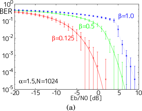
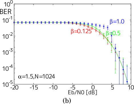
Figure 3: (a) Bit error rate $\mathrm{BER}_{m}$ for messages and (b) $\mathrm{BER}_{R}$ for image. The smooth parameter is $\alpha=1.5$. The embedding rates are $\beta=0.125,0.5,1.0.$

Next, we evaluate the bit error rate for the smooth parameters $\alpha=1.0,1.5$, and $3.0$ under the fixed embedding rate $\beta$. Figure 4 shows the BERs for the embedding rate $\beta=0.5$. Because of the fixed embedding rate, the $\mathrm{BER}_{m}$ for the messages were slightly influenced by the parameter $\alpha$, while the $\mathrm{BER}_{R}$ for the images became better according to $\alpha$. In other words, smoother images can be easily restored.

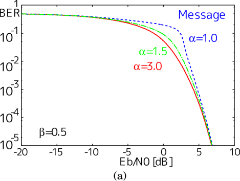
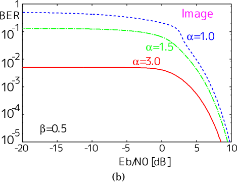
Figure 4: (a) Bit error rate $\mathrm{BER}_{m}$ for messages and (b) $\mathrm{BER}_{R}$ for image. The smooth parameters are $\alpha=1.0,1.5,3.0$. The embedding rate is $\beta=0.5$.

IV.3 Advantages of image restoration

The key concept underlying the proposed method is that it can estimate both the messages and image at the same time in the decoder. Here, we compare the performance of the blind decoder with that of the informed decoder. Cases in which the original image is known or informed to the decoder correspond to the CDMA model, and only messages are estimated.

Figure 5 shows the bit error rate $\mathrm{BER}_{m}$ for messages in the blind and informed decoders. The embedding rates are $\beta=0.125,0.5$, and $1.0$. The BERs in the blind decoder are larger than those in the informed decoder because images are also estimated. However, in cases in which the embedding rate $\beta$ is small enough, or in which there is not much noise in the communication channel, there is not much difference between the blind and informed decoders, i.e., blind decoder can successfully carry out image estimation.

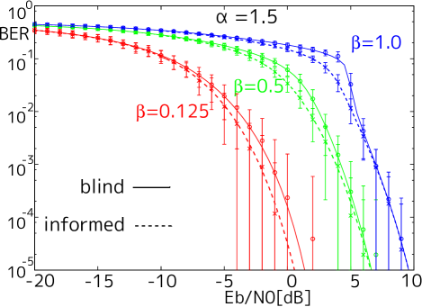
Figure 5: $\mathrm{BER}_{m}$ in the cases of blind and informed images.

IV.4 2D Ising Model

In addition to the infinite range model, we also consider the 2D Ising model for image restoration, in which each pixel is statically connected with four-neighbors. This model is natural for the image restoration. In this model, there are some clusters in generated images because the pixels interact with their nearest neighbors. These cluster patterns can be seen in the parity of JPEG images. In this section, we treat the 2D Ising model as an image generating model; that is, the prior probability is given by

$$P\left(\bm{f}\right) \propto \exp\left[\alpha_{0}\sum_{\left<\mu,\nu\right>}f_{\mu}f_{\nu}\right],$$ (76)

where $\left<\mu,\nu\right>$ denotes pairs of nearest neighbor sites. Figure 6 shows the generated images for parameters $\alpha_{0}=0.4,1.5$, and $10$ in the 2D Ising model. In this manner, once the generating models have been changed, the generated images are much different. Since it is difficult to construct a generating model of natural images, it is necessary to consider various generating models in which as many characteristics of natural images are applied as possible.

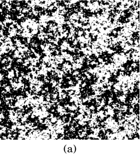
Figure 6: Images generated by 2D-Ising model ($256\times 256$ pixels) with the smooth parameters (a) $\alpha_{0}=0.4$, (b) $\alpha_{0}=1.5$, and (c) $\alpha_{0}=10.0$.

The posterior probability of the original image $\bm{f}$ given the tampered image $\bm{r}$ is given by

$$P\left(\bm{f}|\bm{r}\right) = \frac{1}{Z}\exp\left[-\frac{1}{2\sigma^{2}}\sum_{\mu=1}^{N}\left(r_{\mu}-f_{\mu}\right)^{2}+\alpha\sum_{\left<\mu,\nu\right>}f_{\mu}f_{\nu}\right].$$ (77)

Although the replica method can be applied to a certain 2D Ising model with diluted random connections by using a mean field approximation EdwardsAnderson1975 , the exact treatment of the 2D Ising model is technically difficult and the replica method does not yield the accurate assessment. We therefore evaluate its performance by computer simulations. Since we can see the continuous structure in Fig. 6, the image size in the 2D Ising model is $256\times 256$ pixels unlike ones of the infinite range model. The images are divided into $256$ blocks, whose size is $256$ pixels per a block. So, the spread code length is $N=256$. Figure 7 shows the bit error rates $\mathrm{BER}_{m}$ and $\mathrm{BER}_{R}$ for the 2D Ising model. The parameters $\alpha$ and $\sigma^{2}$ are set to the true value $\alpha=\alpha_{0}$ and $\sigma^{2}=\sigma_{0}^{2}$. The BERs are averaged over all blocks. $\mathrm{BER}_{R}$ for the images are slightly influenced by the embedding rate $\beta$ under the fixed parameter $\alpha$.

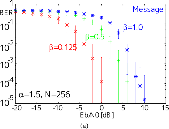
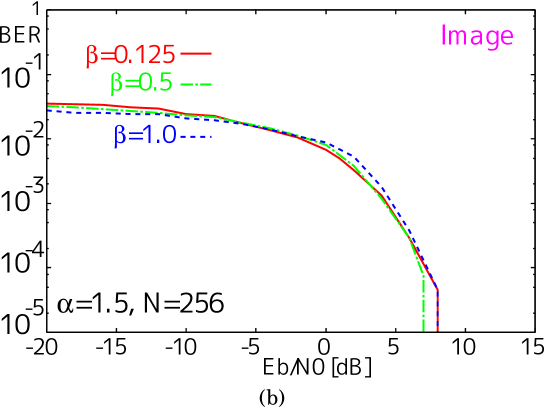
Figure 7: (a) Bit error rates $\mathrm{BER}_{m}$ for messages and (b) $\mathrm{BER}_{R}$ for image in 2D Ising model. The smooth parameter is $\alpha=\alpha_{0}=1.5$. The embedding rates are $\beta=0.125,0.5,1.0$.

Next, we evaluate the performance under the fixed embedding rate $\beta=0.25$. Figure 8 shows BERs for the smooth parameters $\alpha_{0}=0.4,1.5$, and $10.0$. $\mathrm{BER}_{m}$ for messages are slightly influenced by $\alpha$. $\mathrm{BER}_{R}$ for images in cases of $\alpha_{0}>1$ are smaller than those of $\alpha=0.4$. For large $\alpha_{0}=10$, phase transition may occure.

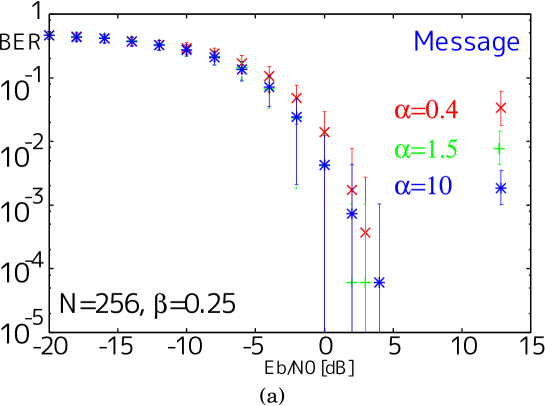
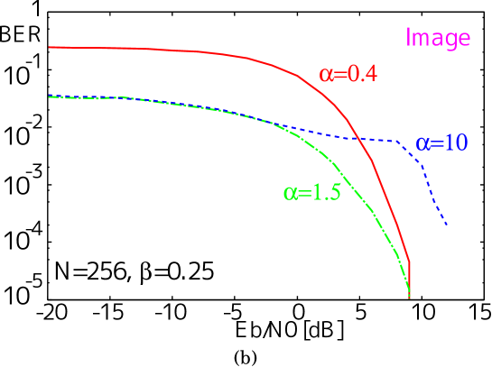
Figure 8: (a) Bit error rate $\mathrm{BER}_{m}$ for messages and (b) $\mathrm{BER}_{R}$ for image in 2D Ising model. The smooth parameters are $\alpha_{0}=0.4,1.5$, $10.0$. The embedding rate is $\beta=0.25$.

Figure 9 shows the bit error rate $\mathrm{BER}_{m}$ for messages in both blind and informed decoders. The embedding rates were $\beta=0.125,0.5$, and $1.0$. Curved lines denote the theoretical values for the informed decoder. The blind decoder had just as good a performance as the informed decoder. That is, the blind decoder could successfully restore the image and estimate the messages.

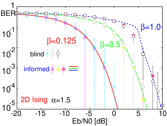
Figure 9: $\mathrm{BER}_{m}$ in blind and informed cases. The smooth parameter is $\alpha=1.5$. The embedding rates are $\beta=0.125,0.5$, $1.0$.

V Conclusion

We proposed an estimation method that can estimate messages and an image at the same time when using a blind decoder. When this method is used with Bayes estimation, prior probabilities for both the messages and the images are required. In this paper, we assumed that the prior probability for messages had a uniform distribution and that those for images were the infinite range model and 2D Ising model.

For the infinite range model, we derived the saddle point equations by the replica method in order to evaluate the average performance. Since there are two terms – the messages term and the image term – we implemented a two-step approach: first, we introduced order parameters for the messages and assumed replica symmetry for them, and second, we introduced order parameters for the image and assumed replica symmetry for them. The obtained saddle point equations consist of two indivisible parts: the equations of the CDMA model and those of the image restoration model. We verified the saddle point equations by computer simulations. The theoretical results agreed with those of the simulations.

Next, we evaluated the performance of the 2D Ising model by computer simulations. When the smooth parameter $\alpha_{0}$ was fixed, there was little change in the bit error rate (BER) for images, and the BER for messages depended on the embedding rate $\beta$. In contrast, when the embedding rate $\beta$ was fixed, there was little change in the BER for messages, and the BER for images depended on the smooth parameter. However, there was a lower bound in the 2D Ising model.

We also evaluated the performance differences between blind and informed decoders. Results showed that the difference was very small when the embedding or attack rates were small, since the image restoration could still be carried out well. This demonstrates the effectiveness of the proposed method.

Appendix A Integral of $[Z^{n}]$ with respect to $r_{\mu},v_{0}^{\mu},\widehat{v}^{\mu}_{0}$

From (36), we obtain

$$\left[Z^{n}\right] = \int\prod_{a<b}\frac{idq_{ab}d\widehat{q}_{ab}}{2\pi}\prod_{a}\frac{idm_{a}d\widehat{m}_{a}}{2\pi}e^{N(G_{1}+G_{2}+G_{3})},$$ (78)

where

$$e^{G_{1}} = \exp\left[-\beta\sum_{a<b}\widehat{q}_{ab}q_{ab}-\beta\sum_{a}\widehat{m}_{a}m_{a}\right],$$ (79)

$$e^{NG_{2}} = \mathrel{\mathop{\mbox{Tr}~{}}\limits_{\small\bm{s},\bm{x}}}\prod_{k=1}^{K}\exp\left[\sum_{a<b}\widehat{q}_{ab}x_{k}^{a}x_{k}^{b}+\sum_{a}\widehat{m}_{a}s_{k}x_{k}^{a}\right],$$ (80)

$$e^{NG_{3}} = \mathrel{\mathop{\mbox{Tr}~{}}\limits_{\small\bm{f},\bm{g}}}\prod_{\mu}\int\frac{dv^{\mu}_{0}d\widehat{v}^{\mu}_{0}}{2\pi}\prod_{a}\frac{dv^{\mu}_{a}d\widehat{v}^{\mu}_{a}}{2\pi}\frac{dr_{\mu}}{\sqrt{2\pi}\sigma_{0}}\exp\left[i\widehat{v}^{\mu}_{0}v^{\mu}_{0}+i\sum_{a}\widehat{v}^{\mu}_{a}v^{\mu}_{a}-\frac{1}{2}\sum_{a}(\widehat{v}^{\mu}_{a})^{2}-\frac{1}{2}(\widehat{v}^{\mu}_{0})^{2}\right.$$ (81)

$$\left.-\sum_{a<b}q_{ab}\widehat{v}_{a}\widehat{v}_{b}-\sum_{a}m_{a}\widehat{v}_{0}\widehat{v}_{a}-\frac{1}{2\sigma_{0}^{2}}\left(r_{\mu}-v^{\mu}_{0}-f_{\mu}\right)^{2}-\frac{1}{2\sigma^{2}}\sum_{a}\left(r_{\mu}-v^{\mu}_{a}-g_{\mu}^{a}\right)^{2}\right.$$

$$\left.+\frac{\alpha_{0}}{N}\sum_{\mu<\nu}f_{\mu}f_{\nu}+\frac{\alpha}{N}\sum_{a=1}^{n}\sum_{\mu<\nu}g_{\mu}^{a}g_{\nu}^{a}\right],$$

Now, we integrate $e^{NG_{3}}$ by $r_{\mu},v_{0}^{\mu},\widehat{v}^{\mu}_{0}$:

$$e^{NG_{3}}$$ (82)

$$= \mathrel{\mathop{\mbox{Tr}~{}}\limits_{\small\bm{f},\bm{g}}}\prod_{\mu}\sqrt{\frac{\sigma^{2}}{\sigma^{2}+n(\sigma_{0}^{2}+1)}}\int\prod_{a}\frac{dv^{\mu}_{a}d\widehat{v}^{\mu}_{a}}{2\pi}\int D_{t_{\mu}}\exp\left[-\frac{1}{2\sigma^{2}}\sum_{a}(v^{\mu}_{a})^{2}+i\sum_{a}\widehat{v}^{\mu}_{a}v^{\mu}_{a}-\frac{1}{2}\sum_{a}(\widehat{v}^{\mu}_{a})^{2}\right.$$

$$+\left\{t_{\mu}\sqrt{\frac{\sigma_{0}^{2}+1}{\sigma^{2}\{\sigma^{2}+n(\sigma_{0}^{2}+1)\}}}+\frac{1}{\sigma^{2}+n(\sigma_{0}^{2}+1)}\left(-i\sum_{a}m_{a}\widehat{v}^{\mu}_{a}+f_{\mu}+\frac{\sigma_{0}^{2}+1}{\sigma^{2}}\sum_{a}g^{a}_{\mu}\right)\right\}\sum_{a}v^{\mu}_{a}$$

$$-\frac{1}{\sigma^{2}}\sum_{a}g_{\mu}^{a}v^{\mu}_{a}+\frac{n}{2\{\sigma^{2}+n(\sigma_{0}^{2}+1)\}}\left(\sum_{a}m_{a}\widehat{v}^{\mu}_{a}\right)^{2}+\frac{in}{\sigma^{2}+n(\sigma_{0}^{2}+1)}f_{\mu}\sum_{a}m_{a}\widehat{v}^{\mu}_{a}$$

$$\left.+\frac{1}{\sigma^{2}+n(\sigma_{0}^{2}+1)}\left(-i\sum_{a}m_{a}\widehat{v}^{\mu}_{a}+f_{\mu}\right)\sum_{a}g^{a}_{\mu}+\frac{\sigma_{0}^{2}+1}{2\sigma^{2}\{\sigma^{2}+n(\sigma_{0}^{2}+1)\}}\left(\sum_{a}g^{a}_{\mu}\right)^{2}\right.$$

$$\left.-\sum_{a<b}q_{ab}\widehat{v}^{\mu}_{a}\widehat{v}^{\mu}_{b}+\frac{\alpha_{0}}{N}\sum_{\mu<\nu}f_{\mu}f_{\nu}+\frac{\alpha}{N}\sum_{a=1}^{n}\sum_{\mu<\nu}g_{\mu}^{a}g_{\nu}^{a}\right].$$

Under the assumption of the replica symmetry, we obtain

$$e^{NG_{3}}$$ (83)

$$= \mathrel{\mathop{\mbox{Tr}~{}}\limits_{\small\bm{f},\bm{g}}}\prod_{\mu}\sqrt{\frac{\sigma^{2}}{\sigma^{2}+n(\sigma_{0}^{2}+1)}}\int\prod_{a}\frac{dv^{\mu}_{a}d\widehat{v}^{\mu}_{a}}{2\pi}\int D_{t_{\mu}}\exp\left[-\frac{1}{2\sigma^{2}}\sum_{a}(v^{\mu}_{a})^{2}+i\sum_{a}\widehat{v}^{\mu}_{a}v^{\mu}_{a}-\frac{1}{2}\sum_{a}(\widehat{v}^{\mu}_{a})^{2}\right.$$

$$+\left\{t_{\mu}\sqrt{\frac{\sigma_{0}^{2}+1}{\sigma^{2}\{\sigma^{2}+n(\sigma_{0}^{2}+1)\}}}+\frac{1}{\sigma^{2}+n(\sigma_{0}^{2}+1)}\left(-im\sum_{a}\widehat{v}^{\mu}_{a}+f_{\mu}+\frac{\sigma_{0}^{2}+1}{\sigma^{2}}\sum_{a}g^{a}_{\mu}\right)\right\}\sum_{a}v^{\mu}_{a}$$

$$-\frac{1}{\sigma^{2}}\sum_{a}g_{\mu}^{a}v^{\mu}_{a}+\frac{nm^{2}}{2\{\sigma^{2}+n(\sigma_{0}^{2}+1)\}}\left(\sum_{a}\widehat{v}^{\mu}_{a}\right)^{2}+\frac{inm}{\sigma^{2}+n(\sigma_{0}^{2}+1)}f_{\mu}\sum_{a}\widehat{v}^{\mu}_{a}$$

$$\left.+\frac{1}{\sigma^{2}+n(\sigma_{0}^{2}+1)}\left(-im\sum_{a}\widehat{v}^{\mu}_{a}+f_{\mu}\right)\sum_{a}g^{a}_{\mu}+\frac{\sigma_{0}^{2}+1}{2\sigma^{2}\{\sigma^{2}+n(\sigma_{0}^{2}+1)\}}\left(\sum_{a}g^{a}_{\mu}\right)^{2}\right.$$

$$\left.-\frac{q}{2}\left\{\left(\sum_{a}\widehat{v}^{\mu}_{a}\right)^{2}-\sum_{a}\left(\widehat{v}^{\mu}_{a}\right)^{2}\right\}+\frac{\alpha_{0}}{2N}\left(\sum_{\mu=1}^{N}f_{\mu}\right)^{2}-\frac{\alpha_{0}}{2}+\frac{\alpha}{2N}\sum_{a=1}^{n}\left(\sum_{\mu=1}^{N}g_{\mu}^{a}\right)^{2}-\frac{\alpha}{2}\right].$$

Appendix B Integral of $e^{NG_{3}}$ with respect to $v^{\mu}_{a},\widehat{v}^{\mu}_{a}$

Under the assumption of the replica symmetry, we integrate by $v^{\mu}_{a}$, and eliminate the terms at the limit $n\to 0$. We obtain

$$e^{NG_{3}}=\mathrel{\mathop{\mbox{Tr}~{}}\limits_{\small\bm{f},\bm{g}}}\prod_{\mu}\sqrt{\frac{\sigma^{2}}{\sigma^{2}+n(\sigma_{0}^{2}+1)}}\int\prod_{a}\frac{dv^{\mu}_{a}d\widehat{v}^{\mu}_{a}}{2\pi}\int D_{t_{\mu}}\exp\left[-\frac{1}{2\sigma^{2}}\sum_{a}(v^{\mu}_{a})^{2}+i\sum_{a}\widehat{v}^{\mu}_{a}v^{\mu}_{a}\right.$$ (85)

$$+\left\{t_{\mu}\sqrt{\frac{\sigma_{0}^{2}+1}{\sigma^{2}\{\sigma^{2}+n(\sigma_{0}^{2}+1)\}}}+\frac{1}{\sigma^{2}+n(\sigma_{0}^{2}+1)}\left(-im\sum_{a}\widehat{v}^{\mu}_{a}+f_{\mu}+\frac{\sigma_{0}^{2}+1}{\sigma^{2}}\sum_{a}g^{a}_{\mu}\right)\right\}\sum_{a}v^{\mu}_{a}$$

$$-\frac{1}{\sigma^{2}}\sum_{a}g_{\mu}^{a}v^{\mu}_{a}-\frac{1}{2}\left(1-q\right)\sum_{a}(\widehat{v}^{\mu}_{a})^{2}+\left\{\frac{nm^{2}}{2\{\sigma^{2}+n(\sigma_{0}^{2}+1)\}}-\frac{q}{2}\right\}\left(\sum_{a}\widehat{v}^{\mu}_{a}\right)^{2}$$

$$+\frac{im}{\sigma^{2}+n(\sigma_{0}^{2}+1)}\left(nf_{\mu}-\sum_{a}g^{a}_{\mu}\right)\sum_{a}\widehat{v}^{\mu}_{a}+\frac{1}{\sigma^{2}+n(\sigma_{0}^{2}+1)}f_{\mu}\sum_{a}g^{a}_{\mu}$$

$$\left.+\frac{\sigma_{0}^{2}+1}{2\sigma^{2}\{\sigma^{2}+n(\sigma_{0}^{2}+1)\}}\left(\sum_{a}g^{a}_{\mu}\right)^{2}+\frac{\alpha_{0}}{2N}\left(\sum_{\mu=1}^{N}f_{\mu}\right)^{2}+\frac{\alpha}{2N}\sum_{a=1}^{n}\left(\sum_{\mu=1}^{N}g_{\mu}^{a}\right)^{2}\right],$$

$$= \mathrel{\mathop{\mbox{Tr}~{}}\limits_{\small\bm{f},\bm{g}}}\prod_{\mu}\sigma^{n}\int\prod_{a}\frac{d\widehat{v}^{\mu}_{a}}{\sqrt{2\pi}}\int D_{t_{\mu}}\exp\left[-\frac{1}{2}\left(\sigma^{2}+1-q\right)\sum_{a}(\widehat{v}^{\mu}_{a})^{2}+\left(m-\frac{q}{2}\right)\left(\sum_{a}\widehat{v}^{\mu}_{a}\right)^{2}\right.$$

$$+\frac{inm}{\sigma^{2}}f_{\mu}\sum_{a}\widehat{v}^{\mu}_{a}-i\sum_{a}g_{\mu}^{a}\widehat{v}^{\mu}_{a}+i\left(1-\frac{nm}{\sigma^{2}}\right)\left(f_{\mu}+\frac{\sigma_{0}^{2}+1}{\sigma^{2}}\sum_{b}g_{\mu}^{b}+t_{\mu}\sqrt{\sigma_{0}^{2}+1}\right)\sum_{a}\widehat{v}^{\mu}_{a}$$

$$+\frac{n}{2\sigma^{2}}\left(f_{\mu}+\frac{\sigma_{0}^{2}+1}{\sigma^{2}}\sum_{a}g_{\mu}^{a}\right)^{2}-\frac{\sigma_{0}^{2}+1}{2\sigma^{4}}\left(\sum_{a}g^{a}_{\mu}\right)^{2}$$

$$+\frac{nt_{\mu}\sqrt{\sigma_{0}^{2}+1}}{\sigma^{2}}\left(f_{\mu}+\frac{\sigma_{0}^{2}+1}{\sigma^{2}}\sum_{a}g_{\mu}^{a}\right)-\frac{t_{\mu}\sqrt{\sigma_{0}^{2}+1}}{\sigma^{2}}\sum_{a}g_{\mu}^{a}+\frac{nt_{\mu}^{2}(\sigma_{0}^{2}+1)}{2\sigma^{2}}$$

$$\left.+\frac{\alpha_{0}}{2N}\left(\sum_{\mu=1}^{N}f_{\mu}\right)^{2}+\frac{\alpha}{2N}\sum_{a=1}^{n}\left(\sum_{\mu=1}^{N}g_{\mu}^{a}\right)^{2}\right].$$

Using Hubbard-Stratonovich transformation,

$$\exp\left[\left(m-\frac{q}{2}\right)\left(\sum_{a}\widehat{v}^{\mu}_{a}\right)^{2}\right] = \int D_{z_{\mu}}\exp\left[z_{\mu}\sqrt{2m-q}\sum_{a}\widehat{v}^{\mu}_{a}\right],$$ (86)

we integrate by $\widehat{v}^{\mu}_{a},t_{\mu},z_{\mu}$:

$$e^{NG_{3}} = \mathrel{\mathop{\mbox{Tr}~{}}\limits_{\small\bm{f},\bm{g}}}\prod_{\mu}\sigma^{n}\left(\sigma^{2}+1-q\right)^{-\frac{n}{2}}\left\{1+\frac{n(2m-q-\sigma_{0}^{2}-1)}{2(\sigma^{2}+1-q)}+\frac{n(\sigma_{0}^{2}+1)}{2\sigma^{2}}+\Upsilon\left(\sum_{a}g_{\mu}^{a}\right)^{2}\right\}$$ (87)

$$\times\exp\left[\Phi+\Psi\sum_{a<b}g_{\mu}^{a}g_{\mu}^{b}+\Omega f_{\mu}\sum_{a}g_{\mu}^{a}+\frac{\alpha_{0}}{2N}\left(\sum_{\mu=1}^{N}f_{\mu}\right)^{2}+\frac{\alpha}{2N}\sum_{a}\left(\sum_{\mu=1}^{N}g_{\mu}^{a}\right)^{2}\right],$$

where

$$\Upsilon = \frac{1}{2}\left\{-\frac{2m-q-\sigma_{0}^{2}-1}{(\sigma^{2}+1-q)^{2}}+\frac{2(\sigma_{0}^{2}+1)\left(1-\frac{nm}{\sigma^{2}}\right)}{\sigma^{2}(\sigma^{2}+1-q)}+\frac{\sigma_{0}^{2}+1}{\sigma^{4}}\right\},$$ (88)

$$\Phi = n\left\{\frac{\sigma_{0}^{2}+1}{\sigma^{2}(\sigma^{2}+1-q)}\left(1-\frac{nm}{\sigma^{2}}\right)-\frac{\sigma_{0}^{2}+1}{2\sigma^{4}}-\frac{1}{\sigma^{2}+1-q}\right\},$$ (89)

$$\Psi = \frac{\sigma_{0}^{2}+1}{\sigma^{2}(\sigma^{2}+1-q)}\left(1-\frac{nm}{\sigma^{2}}\right)\left\{2-\frac{n(\sigma_{0}^{2}+1)}{\sigma^{2}}\left(1-\frac{nm}{\sigma^{2}}\right)\right\}-\frac{\sigma_{0}^{2}+1}{\sigma^{4}},$$ (90)

$$\Omega = \frac{1}{\sigma^{2}+1-q}\left\{1-n(\sigma_{0}^{2}+1)\left(1-\frac{nm}{\sigma^{2}}\right)^{2}\right\}+\frac{n(\sigma_{0}^{2}+1)}{\sigma^{4}}.$$ (91)