Condensation in the inhomogeneous zero-range process: an interplay between interaction and diffusion disorder

Abstract

We analyze the role of the interplay between on-site interaction and inhomogeneous diffusion on the phenomenon of condensation in the zero-range process. We predict a universal phase diagram in the plane of two exponents, respectively characterizing the interactions and the diffusion disorder. The most prominent outcome is the existence of an extended condensed phase. In the latter phase, which originates as a result of the combined effects of strong enough interaction and weak enough disorder, a typical high-density configuration has a unique condensate on top of a critical background, but the condensate may be located at any site of a large hosting set of favored sites, whose size grows sub-extensively. The novel extended condensed phase thus interpolates continuously between the two scenarios associated so far with the condensation transition, namely spontaneous symmetry breaking and explicit symmetry breaking.

,

1 Introduction

The essence of the zero-range process (ZRP) can be best understood by returning to the original work of Spitzer [1]. The starting point is to consider an assembly of independent particles diffusing on a graph, i.e., a finite connected set of $M$ sites. The particles, which we can also refer to as random walkers, are also in finite number, $N$. Choosing a continuous-time description of the process, any individual particle hops from site $m$ to site $n$ with a rate $w_{mn}$. In the course of time, the probabilities for the particle to be at the various sites $m$ relax to the unique normalized solutions $q_{m}$ of the stationary master equation

$$\sum_{n=1}^{M}w_{nm}q_{n}=q_{m}\sum_{n=1}^{M}w_{mn}.$$ (1.1)

For the assembly of independent random walkers, if at time $t$ the occupation of site $m$ is equal to $k$, then, of course, the chance of seeing a particle hop from this site to site $n$ is enhanced by a factor $k$, which amounts to multiplying the hopping rate $w_{mn}$ by $k$. The intention stated by Spitzer was to depart from the field of independent random walkers by introducing a form of interaction between them. In Spitzer’s original definition of the zero-range process, the rate $k\,w_{mn}$ for the hopping of a particle from site $m$, with occupation equal to $k$, to site $n$, which holds if the particles are independent, is changed to the product

$$W(m,n,k)=w_{mn}\,u_{k},$$ (1.2)

where the factor $u_{k}$ only depends on the occupation $k$ of the departure site $m$ at the current time. This dependence gives an explicit content to the denomination of the process as ‘zero-range’. This very definition of the ZRP demonstrates the importance and respective roles of the two facets of this process: diffusion on the one hand, interaction on the other hand. The first one is encoded in the single-particle hopping rate $w_{mn}$, while the second one is encoded in the on-site interaction factor $u_{k}$. Either factor of the product (1.2) can be separately normalized in an arbitrary way (see below (2.5)). This justifies that either factor will sometimes be referred to as a ‘rate’.

The interest of the statistical physics community for the ZRP came long after the publication of [1] and the subsequent works of mathematicians on the subject [2, 3]. The popularity of the ZRP was triggered by the ubiquity of the phenomenon of condensation in a number of processes related in one way or another to the ZRP (for reviews, see [4, 5, 6]). The condensation transition manifests itself by the existence of a critical density $\rho_{c}$, with the following meaning. Consider the stationary state of the model in the thermodynamic limit where $M$ and $N\to\infty$, at fixed density $\rho=N/M$. If the density is high enough ($\rho>\rho_{c}$), a macroscopic (extensive) number of excess particles, of order

$$\Delta=N-M\rho_{c}=M(\rho-\rho_{c}),$$ (1.3)

concentrates on a single site with very high probability.

In the present work we analyze the role of the interplay between the two facets of the ZRP, diffusion and interaction, on the phenomenon of condensation. More precisely, we consider the ZRP defined by the rate (1.2) on a finite system of $N$ particles living on $M$ sites, with the following specifications.

• Diffusion disorder. The single-particle weights $q_{m}$ given by (1.1) enter the factorized form (2.4) of the stationary distribution of the occupations. Rather than explicitly modeling diffusion disorder by endowing a given structure with random hopping rates $w_{mn}$ and calculating the single-particle weights $q_{m}$ through (1.1), we instead assume that the $q_{m}$ can be modeled as independent random variables drawn from a given distribution. We will expand on the motivation for this assumption in section 2.4. More precisely, we characterize the inhomogeneity of the diffusion process by modeling the $q_{m}$ as i.i.d. random variables drawn from the continuous distribution

  $$f(q)=c(1-q)^{c-1}\qquad(0<q<1),$$ (1.4)

  with a power-law singularity as $q\to 1$ with an arbitrary exponent $c>0$, to be referred to as the disorder exponent. The shape of the distribution $f(q)$ in the vicinity of the maximum (supposed to be finite and set here to $q_{\rm max}=1$) will play a central role in the analysis of the condensation transition.

• Interaction. We choose for the factor $u_{k}$, which encodes the interaction between particles sitting at the same site, the form

  $$u_{k}=1+\frac{b}{k},$$ (1.5)

  where $b$ is a parameter describing the strength of on-site interactions, to be referred to as the interaction exponent.

The above model contains as limiting cases two known models exhibiting a condensation phenomenon (see references below).

• Homogeneous ZRP. If diffusion is homogeneous ($q_{m}=1$ for all $m$, i.e., $f(q)=\delta(q-1)$, or formally $c=0$), the process with rate (1.5) is known to have a condensation transition at the critical density

  $$\rho_{c}=\frac{1}{b-2},$$ (1.6)

  whenever the interactions are sufficiently attractive ($b>2$). In this situation, the condensate can sit on any site with equal probabilities in the stationary state of the system. This condensation scenario therefore corresponds to a spontaneous symmetry breaking (SSB) of the symmetry between the sites.

• Occupation-independent inhomogeneous ZRP. If the rate $u_{k}$ is occupation-independent ($u_{k}=1$, i.e., $b=0$), the process with inhomogeneous diffusion described by the distribution (1.4) is also known to have a condensation transition, at the critical density

  $$\rho_{c}=\frac{1}{c-1},$$ (1.7)

  whenever the disorder is sufficiently strong ($c>1$). In this situation the condensate is typically located on the site with the largest single-particle weight. This corresponds to a scenario of explicit symmetry breaking (ESB).

The full model defined by diffusion disorder (1.4) and interaction (1.5) interpolates between the two limiting cases recalled above. The aim of this work is to investigate to what extent the condensation transition of the homogeneous ZRP defined in (i) is altered by the presence of inhomogeneous diffusion, i.e., of the non-trivial distribution (1.4) of the single-particle weights $q_{m}$, or, conversely, how the condensation transition of the inhomogeneous ZRP defined in (ii) is altered by the presence of an interaction corresponding to the rate (1.5).

An informal account of our results is as follows. We show in figure 1 the phase diagram of our model in the plane of the exponents $b$ (characterizing interaction) and $c$ (characterizing disorder). In the fluid phase, there is no condensate at any density. In the localized condensed phase, for any $\rho>\rho_{c}$, a condensate of size $\Delta$ (see (1.3)) lives on the site with the largest single-particle weight with very high probability. In the extended condensed phase, for any $\rho>\rho_{c}$, the condensate is still unique with very high probability, but it may be located at any site of a large hosting set of favored sites, whose size $R$ grows sub-extensively as

$$R\sim\frac{M}{\Delta^{c}}\sim\frac{M^{1-c}}{(\rho-\rho_{c})^{c}}.$$ (1.8)

The existence of an extended condensed phase is the most salient novel feature put forward in the present work. The latter phase implements a continuous interpolation between the two symmetry breaking scenarios recalled above, namely SSB in the homogeneous ZRP ($c=0$, $b>2$), and ESB in the occupation-independent inhomogeneous ZRP ($b=0$, $c>1$). These two limiting scenarios are consistently recovered as $R=M$ and $R=1$, respectively. The ESB scheme more generally applies to the ZRP with $c>1$ and any $b$. Figure 2 shows a more refined phase diagram, where the condensed phases are further divided into a regime of normal fluctuations, where the mean square occupation $\mu_{c}$ at criticality is finite, so that the size fluctuations of the condensate around its mean size $\Delta$ are Gaussian and grow as $M^{1/2}$, and a regime of anomalous fluctuations, where $\mu_{c}$ is divergent, so that size fluctuations are not Gaussian and grow faster than $M^{1/2}$. The phase diagrams depicted in figures 1 and 2 are universal, in the sense that they hold for any rate whose asymptotic behavior at large $k$ is of the form $u_{k}\approx 1+b/k$, and for any distribution of single-particle weights exhibiting a finite maximum $q_{\rm max}$ and a power-law singularity $f(q)\sim(q_{\rm max}-q)^{c-1}$ near this maximum.

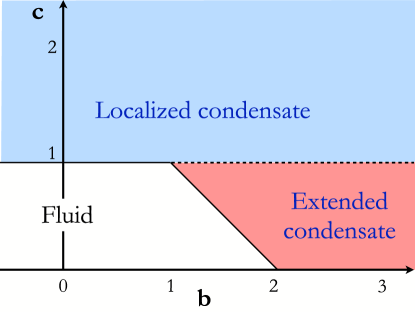
Figure 1: Universal phase diagram of the inhomogeneous ZRP in the $b$–$c$ plane, with its fluid phase and its two condensed phases: a localized one ($c>1$) and a novel extended one ($c<1$).

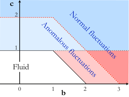
Figure 2: More detailed phase diagram, showing the internal structure of the condensed phases. The size fluctuations of the condensate around its mean $\Delta$ are either normal (finite mean square occupation), or anomalous (divergent mean square occupation).

Before proceeding, let us review the relevant literature.

The homogeneous ZRP with rate (1.5) has been studied in a long series of works, and is by now well understood [4, 5, 6]. The main features of the statics of the model without reference to a dynamical process were first analyzed in [7]. The underlying dynamical process was introduced in [8], where the coarsening dynamics leading to condensation was studied in the mean-field geometry of the complete graph. This study was subsequently pursued in [9]. The relationship of the equilibrium state of the model described in [7] to the stationary state of a ZRP was recognized in [11] and a first analysis of the criterion on the form of the rate $u_{k}$ for condensation to occur was given. This analysis was subsequently completed in [4]. Independently, a similar analysis was performed in [12], devoted to a study of the size of the condensate. Further studies involve the analysis of the coarsening process leading to condensation in the one-dimensional case [10, 13], or on the complete graph [10], the proof of the uniqueness of the condensate and the equivalence of ensembles [13], the analysis of the motion of the condensate at stationarity [14], the analysis of finite-size effects in the canonical ensemble [15], and the relationship of the condensation phenomenon to extreme-value statistics [16]. More mathematical works on similar subjects can be found in [17, 18, 19].

The occupation-independent ZRP with rate $u_{k}=1$ and inhomogeneous diffusion described by (1.4) can be traced back to studies of one-dimensional disordered totally asymmetric exclusion models [20, 21, 22], where the connections with the ZRP [20, 21] and the relationship to Bose-Einstein condensation [22] were recognized. A more mathematical treatment of the condensation transition has been given in [23], while the dynamics of the same model was analyzed in [24], both at stationarity and during the process of the formation of the condensate.

The references cited so far led to the current understanding of the two limiting prototypical cases of the ZRP referred to above. We now turn to other works which deal in some way or another with the interplay of interaction and disorder in the ZRP. The simplest situation of an inhomogeneous ZRP is that of an attractive impurity in a homogeneous background: one site is singled out by its weight $q>1$, while all the other sites keep $q=1$. In this situation condensation occurs even for the occupation-independent ZRP ($u_{k}=1$) [4, 25]. The totally asymmetric one-dimensional inhomogeneous ZRP has been investigated from a rigorous standpoint in [26]. The situation where the diffusion disorder originates in the structure of the underlying graph has also been analyzed [27, 28, 29], the main emphasis being on complex (scale-free) networks. In [27] complete condensation, i.e., $\rho_{c}=0$, has been shown to generally occur on such networks. References [28] also deal with the statics and the dynamics of the occupation-independent ZRP on complex networks. The phenomenon of condensation in disordered urn models has been explored in [30]. The more general case of an inhomogeneous ZRP where disorder enters the interaction part of the rate itself has been recently considered in [31]. Finally, the occupation-independent one-dimensional ZRP with partially asymmetric disordered diffusion has been analyzed in [32]. Reference [33] presents a brief review of the more general area of driven diffusive systems with disorder.

The setup of the present paper is as follows. In section 2, we present some general formalism and emphasize two special situations, namely $u_{k}=k$ (independent random walkers) and $u_{k}=1$ (the occupation-independent case, which can be mapped onto an ideal Bose gas). We then review, in section 3, the two limiting cases of interest recalled above, namely the homogeneous ZRP with rate (1.5) and the occupation-independent inhomogeneous ZRP. Section 4 contains our theoretical investigations, whose main predictions are summarized in the universal phase diagrams depicted in figures 1 and 2. Our quantitative predictions are then illustrated by means of numerical results in section 5. Section 6 presents an application of our findings to the case of complex networks. Section 7 contains a brief discussion, whereas more technical aspects are exposed in three appendices: A contains an investigation of the ZRP on two sites, while B is devoted to the universal fluctuations of the hosting probabilities in the borderline situation ($c=1$), and C to an effective model describing the relevant rare events in the localized regime ($c>1$).

2 General formalism

2.1 Stationary state

We start by a reminder of the definition of the ZRP and of the properties of its stationary state. Consider a finite connected graph of $M$ sites (labelled $m=1,\dots,M$), on which particles hop from site to site in continuous time. We denote by $N_{m}$ the instantaneous occupation of site $m$, i.e., the number of particles living at site $m$ at the current time. The total number of particles in the system,

$$N=\sum_{m=1}^{M}N_{m},$$ (2.1)

is conserved by the dynamics.

According to Spitzer’s original work [1], a ZRP is defined by the following expression (see (1.2))

$$W(m,n,k)=w_{mn}\,u_{k}$$ (2.2)

for the rate for a particle to hop from site $m$ (with occupation $N_{m}=k$) to site $n$, where $w_{mn}$ describes the diffusion of a single particle on the graph, and $u_{k}$ encodes the interaction between particles sitting at the same site. In the present work we focus our attention on an inhomogeneous ZRP defined by (2.2), i.e., with diffusion disorder. For completeness, we mention the following more general definition of a ZRP [5],

$$W(m,n,N_{m})=w_{mn}\,u_{m,k},$$ (2.3)

where the factor $u_{m,k}$ encoding the interaction between the $k$ particles sitting at site $m$ depends explicitly on both $m$ and $k$. References [31] contain an investigation of such a situation, where quenched disorder affects the interactions between particles, and not only the diffusion.

The fundamental property of the ZRP is the simple structure of its stationary state: the distribution of the occupations is factorized. Such a distribution is referred to as a product measure. The particles being considered as indistinguishable, a configuration of the system is entirely defined by the occupations $\{N_{m}\}$. The stationary probability $P(\{N_{m}\})$ of any configuration is given by a product of elementary weights, associated with the occupations of each site. For the hopping rate (1.2) (or (2.2)), we have

$$P(\{N_{m}\})=\frac{1}{Z_{M,N}}\,\prod_{m=1}^{M}q_{m}^{N_{m}}\,p_{N_{m}}\delta\!\left(\sum_{m=1}^{M}N_{m},N\right).$$ (2.4)

The Kronecker delta function ensures the condition (2.1), whereas the normalisation factor $Z_{M,N}$ (see (2.6)) plays the role of a partition function, and the weight associated with each site $m$ is itself a product of the two factors, $q_{m}^{N_{m}}$ and $p_{N_{m}}$. The latter factor is given by

$$p_{0}=1,\qquad p_{k}=\frac{1}{u_{1}\dots u_{k}}.$$ (2.5)

As long as one is only interested in static properties, either factor of the rate (1.2) (or (2.2)) can be normalized in an arbitrary way. Indeed, if all the hopping rates $w_{mn}$ are multiplied by the same constant $A$, the time scale of the dynamical process is changed as $t\to t/A$, but the single-particle weights $q_{m}$ obeying the stationary master equation (1.1) are left unchanged. Similarly, if all the factors $u_{k}$ are multiplied by the same constant $B$, $p_{k}$ is changed to $p_{k}/B^{k}$, the partition function $Z_{M,N}$ gets multiplied by $1/B^{N}$, and so the result (2.4) is unchanged. Furthermore, the single-particle weights themselves can also be normalized in an arbitrary way. Indeed, if all the $q_{m}$ are multiplied by the same constant $C$, $Z_{M,N}$ gets multiplied by $C^{N}$, and so the result (2.4) is again unchanged.

Canonical ensemble.

In the canonical ensemble, the total number $N$ of particles is fixed. The stationary probability $P(\{N_{m}\})$ of any configuration is given by the expression (2.4) above, where the partition function

$$Z_{M,N}=\sum_{\{N_{m}\}}\prod_{m=1}^{M}q_{m}^{N_{m}}\,p_{N_{m}}\,\delta\!\left(\sum_{m=1}^{M}N_{m},N\right)$$ (2.6)

depends on all the $q_{m}$ and all the $p_{k}$.

Singling out the sum over $N_{m}=k$ in (2.6) leads to the recursion relation

$$Z_{M,N}=\sum_{k=0}^{N}q_{m}^{k}\,p_{k}\,Z_{M-1,N-k}({/\!\!\!q}_{m})$$ (2.7)

between partition functions of systems with successive sizes. The argument ${/\!\!\!q}_{m}$ means that $Z_{M-1,N-k}({/\!\!\!q}_{m})$ depend on the $(M-1)$ single-particle weights $q_{n}$ for $n\neq m$. Likewise the distribution of the occupation of site $m$ is obtained from (2.4) as

$$f_{m,k}=\mathop{\rm Prob}\nolimits\{N_{m}=k\}=q_{m}^{k}\,p_{k}\,\frac{Z_{M-1,N-k}({/\!\!\!q}_{m})}{Z_{M,N}}.$$ (2.8)

Hence the mean occupation (local density) at site $m$ reads

$$\rho_{m}=\langle N_{m}\rangle=\sum_{k=0}^{N}kf_{m,k}=\frac{q_{m}}{Z_{M,N}}\,\frac{\partial Z_{M,N}}{\partial q_{m}}=q_{m}\frac{\partial}{\partial q_{m}}\ln Z_{M,N}.$$ (2.9)

The partition function $Z_{M,N}$ being a homogeneous function of degree $N$ of all the $q_{m}$, the sum rule

$$\sum_{m=1}^{M}\rho_{m}=N$$ (2.10)

is ensured by Euler’s identity for homogeneous functions:

$$\sum_{m=1}^{M}q_{m}\,\frac{\partial Z_{M,N}}{\partial q_{m}}=NZ_{M,N}.$$ (2.11)

By using a contour-integral representation of the Kronecker delta function, we can recast the partition function (2.6) into the form

$$Z_{M,N}=\oint\frac{{\rm d}z}{2\pi{\rm i}z^{N+1}}\,{\cal Z}_{M}(z),$$ (2.12)

where the grand partition function reads

$${\cal Z}_{M}(z)=\sum_{N\geq 0}Z_{M,N}z^{N}=\prod_{m=1}^{M}P(zq_{m}),$$ (2.13)

and

$$P(z)=\sum_{k\geq 0}p_{k}z^{k}.$$ (2.14)

Grand-canonical ensemble.

The representation (2.12) of the partition function suggests that one alternatively considers the grand-canonical ensemble, where the fugacity $z$ is fixed, whereas the total number $N$ of particles in the system fluctuates. In that ensemble the stationary distribution of the occupations is strictly a product measure:

$$P^{{\rm GC}}(\{N_{m}\})=\frac{1}{{\cal Z}_{M}(z)}\prod_{m=1}^{M}(zq_{m})^{N_{m}}\,p_{N_{m}}=\prod_{m=1}^{M}f^{{\rm GC}}_{m,k},$$ (2.15)

where the normalized factor $f^{{\rm GC}}_{m,k}$ gives the distribution of the occupation of site $m$:

$$f^{{\rm GC}}_{m,k}=\mathop{\rm Prob}\nolimits\{N_{m}^{{\rm GC}}=k\}=\frac{(zq_{m})^{k}\,p_{k}}{P(zq_{m})}.$$ (2.16)

Thus the mean occupation at site $m$ reads

$$\rho^{{\rm GC}}_{m}=\langle N_{m}^{{\rm GC}}\rangle=\sum_{k\geq 0}kf^{{\rm GC}}_{m,k}=\frac{zq_{m}P^{\prime}(zq_{m})}{P(zq_{m})}=z\frac{\partial}{\partial z}\ln P(zq_{m}),$$ (2.17)

where the accent denotes differentiation, and finally the mean density of the system is

$$\rho^{{\rm GC}}=\frac{\langle N^{{\rm GC}}\rangle}{M}=\frac{1}{M}\sum_{m=1}^{M}\rho^{{\rm GC}}_{m}=\frac{z{\cal Z}^{\prime}_{M}(z)}{M{\cal Z}_{M}(z)}=\frac{z}{M}\frac{\partial}{\partial z}\ln{\cal Z}_{M}(z).$$ (2.18)

2.2 The case of independent random walkers ($u_{k}=k$).

We now turn to the simplest example of a ZRP, corresponding to $u_{k}=k$. As recalled in the introduction, this situation describes independent random walkers. We have

$$p_{k}=\frac{1}{k!},\qquad P(z)=\rme^{z}.$$ (2.19)

Grand-canonical ensemble.

The grand partition function reads

$${\cal Z}_{M}(z)=\rme^{Mz\overline{q}},$$ (2.20)

where we have introduced the notation

$$\overline{q}=\frac{1}{M}\sum_{m=1}^{M}q_{m}$$ (2.21)

for the mean single-particle weight. The occupations therefore follow the Poissonian law

$$f^{{\rm GC}}_{m,k}=\rme^{-zq_{m}}\frac{({zq_{m}})^{k}}{k!},$$ (2.22)

and the local densities read

$$\rho_{m}^{{\rm GC}}=zq_{m}.$$ (2.23)

Thus the mean density and the fugacity are related through

$$\rho^{{\rm GC}}=z\overline{q}.$$ (2.24)

As a consequence, for any density $\rho$, there exists a value of the fugacity, namely $z=\rho/\overline{q}$, such that $\rho^{{\rm GC}}(z)=\rho$. The system can sustain any density of particles and is therefore always in a fluid phase.

Canonical ensemble.

The canonical partition function is

$$Z_{M,N}=\frac{(M\overline{q})^{N}}{N!},$$ (2.25)

and the local densities read

$$\rho_{m}=\frac{Nq_{m}}{M\overline{q}}.$$ (2.26)

The canonical joint distribution of the occupations is multinomial:

$$P(\{N_{m}\})=\frac{1}{(M\overline{q})^{N}}\;\displaystyle{\frac{\displaystyle N!}{\displaystyle\prod_{m=1}^{M}N_{m}!}}\;\prod_{m=1}^{M}q_{m}^{N_{m}},$$ (2.27)

as it should be, since independent random walkers behave as independent classical particles.

2.3 The occupation-independent case ($u_{k}=1$).

The occupation-independent ZRP with $u_{k}=1$ is another simple example, yet richer because the random walkers are no longer independent. We have then

$$p_{k}=1,\qquad P(z)=\frac{1}{1-z}.$$ (2.28)

Grand-canonical ensemble.

The grand partition function reads

$${\cal Z}_{M}(z)=\prod_{m=1}^{M}\frac{1}{1-zq_{m}}.$$ (2.29)

The occupations therefore follow the geometric law

$$f^{{\rm GC}}_{m,k}=(1-zq_{m})(zq_{m})^{k},$$ (2.30)

and the local densities read

$$\rho^{{\rm GC}}_{m}=\frac{zq_{m}}{1-zq_{m}}.$$ (2.31)

Thus the mean density and the fugacity are related through

$$\rho^{{\rm GC}}=\frac{1}{M}\sum_{m=1}^{M}\frac{zq_{m}}{1-zq_{m}}.$$ (2.32)

For a homogeneous system ($q_{m}=1$), this relation simplifies to

$$\rho^{{\rm GC}}=\frac{z}{1-z},$$ (2.33)

which has a solution $z(\rho^{{\rm GC}})$ for any value of the density, and hence the system is again in a fluid phase. However, if the system is inhomogeneous, local densities are given by (2.31), and a condensation transition may occur. The simplest case is that of an attractive impurity [4, 25], where one of the $q_{m}$ is larger than the common value of all the other ones. A condensation transition also occurs in the thermodynamic limit when the $q_{m}$ are random and distributed according to (1.4) with $c>1$. The latter phenomenon is addressed in section 3.2.

It is worth emphasizing the analogy between the statics of the occupation-independent ZRP and that of an ideal Bose gas [5, 22]. Setting $z=\rme^{\beta\mu}$, where $\beta$ is the inverse temperature and $\mu$ the chemical potential, and $q_{m}=\rme^{-\beta E_{m}}$, the expression (2.31) for the local particle density at site $m$ identifies with the Bose occupation factor

$$f_{\rm Bose}(E_{m})=\frac{1}{\rme^{\beta(E_{m}-\mu)}-1}$$ (2.34)

of a fictitious quantum-mechanical level with energy $E_{m}$. Identifying the connection between classical stochastic processes and the ideal Bose gas dates back to [34].

The distribution (1.4) of the single-particle weights translates to a distribution of energy levels (density of states) $D(E)$ vanishing as $D(E)\sim E^{c-1}$ as the energy $E>0$ approaches zero. The latter power-law singularity is to be put in perspective with the density of states of a free particle in a box in $d$-dimensional space, i.e., $D(E)\sim E^{d/2-1}$. This parallel leads to the identification $c=d/2$ between the disorder exponent $c$ and half the dimensionality of the space where the Bose gas lives. The condition $c>1$ for having a condensation transition [21, 22], recalled above and to be worked out in section 3.2, is therefore equivalent to the well-known result that an ideal Bose gas exhibits a Bose-Einstein condensation in dimension $d>2$ only.

Canonical ensemble.

The canonical partition function can be evaluated from the representation (2.12) as

$$Z_{M,N}=\oint\frac{{\rm d}z}{2\pi{\rm i}z^{N+1}}\prod_{m=1}^{M}\frac{1}{1-zq_{m}}.$$ (2.35)

Evaluating the contour integral by the method of residues, we get

$$Z_{M,N}=\sum_{m=1}^{M}q_{m}^{N}Q_{m},$$ (2.36)

with

$$Q_{m}=\prod_{n\neq m}\frac{q_{m}}{q_{m}-q_{n}}.$$ (2.37)

The local densities can then be obtained by differentiating the above formulas according to (2.9). We thus obtain

$$\rho_{m}=\frac{1}{Z_{M,N}}\left(Nq_{m}^{N}Q_{m}+\sum_{n\neq m}\frac{q_{n}q_{m}^{N}Q_{m}+q_{m}q_{n}^{N}Q_{n}}{q_{n}-q_{m}}\right).$$ (2.38)

The expressions (2.36) and (2.38) are much more intricate than their counterparts (2.25) and (2.26) in the case of independent random walkers. This difference can be attributed to the fact that the canonical ensemble is the natural framework to describe identical classical particles (hence the simplicity of the multinomial joint distribution (2.27)), whereas the grand-canonical ensemble is the only natural one when dealing with quantum-mechanical energy levels (hence the analogy between the expression (2.31) for the grand-canonical local density and the Bose occupation factor (2.34)).

2.4 On the choice of single-particle weights made in this work

Let us come back to the specific model considered in the present work. For a given ZRP, defined by the rates $u_{k}$ and $w_{mn}$, the stationary properties only rely on the knowledge of the weights $p_{k}$ and $q_{m}$. The former ones are easily deduced from the rates $u_{k}$ (see (2.5)). In contrast, the stationary master equation (1.1) cannot be solved in closed form in general. The problem indeed belongs to the rich and complex area of diffusion in random media [35]. In this work we have adopted the alternative viewpoint of modeling diffusion disorder by considering the single-particle weights $q_{m}$ as i.i.d. random variables drawn from the distribution (1.4).

Let us take the example of the mean-field geometry of a completely connected graph over $M$ sites to discuss the issue. Consider the inhomogeneous diffusion where the particle leaves site $m$ with some site-dependent rate $\lambda_{m}$, and jumps to a random arrival site $n$, chosen uniformly over the system. We have therefore $w_{mn}=\lambda_{m}/M$. It can be checked that the stationary probabilities read $q_{m}=1/\lambda_{m}$, up to normalization. In the more general situation of separable rates of the form $w_{mn}=\lambda_{m}\mu_{n}$, we have $q_{m}=\mu_{m}/\lambda_{m}$, again up to normalization. The stationary state thus obtained is an equilibrium state, obeying the condition of detailed balance. The mean current from site $m$ to site $n$, $J_{mn}=w_{mn}q_{m}=\mu_{m}\mu_{n}$, up to normalization, is indeed symmetric. Another example is the case of the totally asymmetric diffusion on a one-dimensional lattice, either infinite or finite with periodic boundary conditions, such that $w_{mn}=\lambda_{m}\,\delta_{n,m+1}$. Here again, we have $q_{m}=1/\lambda_{m}$, up to normalization.

In the two above examples of inhomogeneous diffusion, the single-particle weights $q_{m}$ can be viewed as independent random variables, and they can take any prescribed values. This somehow justifies our choice of modeling them by i.i.d. random variables with an arbitrary distribution $f(q)$. It should however be clear that the single-particle weights cannot be viewed as independent random variables in the most general situation. Consider for definiteness a finite-dimensional lattice with weakly disordered asymmetric hopping rates $w_{mn}$ on its bonds. In this case, the $q_{m}$ are given by the normalized solution of the stationary master equation (1.1), which may exhibit a non-trivial spatial structure, especially in the one-dimensional case of the Sinai model [35].

Finally, the rationale for the choice (1.4) of the distribution $f(q)$ of single-particle weights is as follows. The properties of the condensate are dictated by the largest single-particle weights, and therefore by the behavior of the distribution $f(q)$ near its maximum $q_{\rm max}$. The situation where $q_{\rm max}$ is infinite is somehow pathological and requires a case-by-case study. Section 6 contains an investigation of a physically motivated situation of this type, namely complex networks. In the case where $q_{\rm max}$ is finite (and can then be set equal to unity), the situation of a power-law singularity turns out to be the appropriate framework to disclose the phase diagram. If the distribution $f(q)$ vanishes faster than a power law as $q\to q_{\rm max}=1$, then one has formally $c=\infty$, thus, for $\rho>\rho_{c}$ the system will always be in the localized condensed phase, irrespective of the interaction exponent $b$. Finally, the pure power law (1.4) has been chosen merely for simplicity.

3 Two limiting case studies

As mentioned in the introduction, the full model defined by (1.4) and (1.5) contains two limiting prototypical cases which are known to exhibit a condensation transition. We recall here the properties of these models which will be relevant for the study of the full model, to be presented in section 4.

3.1 Homogeneous ZRP: spontaneous symmetry breaking

The homogeneous ZRP (see [4, 5, 6] for reviews) corresponds to the case where the single-particle weights $q_{m}$ are uniform, i.e., do not depend on the site. This homogeneity property holds for the complete graph with uniform hopping rates, and more generally whenever all sites are symmetry-related and thus equivalent. This is automatically satisfied if the sites are related to each other by translation invariance, like e.g. for usual symmetric or biased random walk on finite lattices with periodic boundary conditions.

Consider the homogeneous ZRP with rate (1.5). Setting $q_{m}=1$, we have

$${\cal Z}_{M}(z)=P(z)^{M}.$$ (3.1)

As a consequence, in the grand-canonical ensemble, (2.16) and (2.17) respectively become

$$f^{{\rm GC}}_{k}=\frac{z^{k}p_{k}}{P(z)}$$ (3.2)

and

$$\rho^{{\rm GC}}=\frac{zP^{\prime}(z)}{P(z)}.$$ (3.3)

In the canonical ensemble, in the thermodynamic limit ($M\to\infty$, $N\to\infty$, $\rho=N/M$ fixed), the condition (3.3) is recovered by estimating the contour integral (2.12) by the saddle-point method. This shows that both statistical ensembles are equivalent in the thermodynamic limit as long as the system remains fluid, i.e., provided no condensate appears, as could be expected.

With the rate (1.5), we have

$$p_{k}=\frac{\Gamma(b+1)\,k!}{\Gamma(k+b+1)}=\int_{0}^{1}u^{k}\,b(1-u)^{b-1}\,{\rm d}u\approx\frac{\Gamma(b+1)}{k^{b}},$$ (3.4)

hence

$$P(z)=\int_{0}^{1}\frac{b(1-u)^{b-1}}{1-zu}\,{\rm d}u={}_{2}F_{1}(1,1;b+1;z),$$ (3.5)

where ${}_{2}F_{1}$ is the hypergeometric function.

The following values will be needed in the sequel:

$$P(1)=\displaystyle{\frac{\displaystyle b}{\displaystyle b-1}},\qquad P^{\prime}(1)=\displaystyle{\frac{\displaystyle b}{\displaystyle(b-1)(b-2)}},$$

$$P^{\prime\prime}(1)=\displaystyle{\frac{\displaystyle 4b}{\displaystyle(b-1)(b-2)(b-3)}},$$ (3.6)

where it is understood that these quantities are convergent respectively for $b>1$, $b>2$, and $b>3$. More generally, the function $P(z)$ has a branch cut at $z=1$, with a singular part of the form

$$P_{\rm sg}(z)\approx\displaystyle{\frac{\displaystyle\pi b}{\displaystyle\sin\pi b}}\,(1-z)^{b-1}.$$ (3.7)

Whenever $b$ is a positive integer or a half-integer, $P(z)$ can be expressed in terms of elementary functions. In particular, for every integer $b=n\geq 1$, its singular part is of the form $P_{\rm sg}(z)\approx(-1)^{n}n(1-z)^{n-1}\ln(1-z)$. We have, for instance,

$$b=1 : \quad P(z)=-\frac{\ln(1-z)}{z},$$

$$b=2 : \quad P(z)=\frac{2(1-z)\ln(1-z)}{z^{2}}+\frac{2}{z},$$

$$b=3 : \quad P(z)=-\frac{3(1-z)^{2}\ln(1-z)}{z^{3}}-\frac{3}{z^{2}}+\frac{9}{2z},$$

$$b=4 : \quad P(z)=\frac{4(1-z)^{3}\ln(1-z)}{z^{4}}+\frac{4}{z^{3}}-\frac{10}{z^{2}}+\frac{22}{3z}.$$ (3.8)

The homogeneous ZRP with rate (1.5) has a continuous phase transition when the fugacity $z$ reaches the singular point $z_{c}=1$. For $b>2$, this takes place at a finite critical density (see (1.6))

$$\rho_{c}=\frac{P^{\prime}(1)}{P(1)}=\frac{1}{b-2}.$$ (3.9)

This critical density separates a fluid phase $(\rho<\rho_{c})$ and a condensed phase $(\rho>\rho_{c})$, whose main characteristics are as follows.

• Fluid phase $(\rho<\rho_{c})$. The canonical and grand-canonical ensembles are equivalent throughout the fluid phase. The density $\rho=\rho^{{\rm GC}}$ increases from 0 to $\rho_{c}$ as the fugacity $z$ increases from 0 to 1. The occupation probabilities $f_{k}=f_{k}^{{\rm GC}}$ (see (3.2)) fall off exponentially.

• Critical density $(\rho=\rho_{c})$. This density is reached when the fugacity $z$ takes the singular value $z_{c}=1$. It is therefore the maximal density that can be reached in the grand-canonical ensemble.

  At the critical density, the occupation probabilities

  $$f_{k}=\frac{p_{k}}{P(1)}\approx\frac{(b-1)\Gamma(b)}{k^{b}}$$ (3.10)

  fall off as a power law with exponent $b$. The second moment of the occupation probabilities at criticality,

  $$\mu_{c}=\sum_{k\geq 0}k^{2}f_{k}=\frac{P^{\prime}(1)+P^{\prime\prime}(1)}{P(1)}=\frac{b+1}{(b-2)(b-3)},$$ (3.11)

  is convergent for $b>3$ (regime of normal fluctuations), whereas it is divergent for $2<b<3$ (regime of anomalous fluctuations).

• Condensed phase $(\rho>\rho_{c})$. The condensed phase only exists in the canonical ensemble where the total number $N$ of particles is imposed. A large ZRP in its condensed phase consists of a uniform critical background, characterized by the critical occupation probabilities (3.10), and of a single macroscopic condensate, containing an extensive number of excess particles of order $\Delta=M(\rho-\rho_{c})$ (see (1.3)). For a system where all sites are equivalent, the condensate can be at any site $m$ with probability $1/M$. The fluctuations of the number of particles in the condensate around $\Delta$ are known to be Gaussian and to scale as $M^{1/2}$ in the regime of normal fluctuations ($b>3$), whereas they have a broad distribution and scale as $M^{1/(b-1)}$ in the regime of anomalous fluctuations ($2<b<3$) [13, 15].

For the homogeneous ZRP, the spontaneous symmetry breaking (SSB) scenario in the condensed phase, with its unique condensate on top of a critical background in the thermodynamic limit, has been proved rigorously [13, 17]. The rare configurations where the condensate is not unique, i.e., where the $\Delta$ excess particles are shared by two sites in significant proportions, have been argued to occur with a probability falling off as the power law $1/M^{b-2}$ [14].

Let us close with a comment on universality. The condition $b>2$ for the existence of a condensed phase is universal, in the sense that any rate with asymptotic behavior $u_{k}=1+b/k+\cdots$ yields a finite critical density $\rho_{c}$ only for $b>2$. In contrast, the value of $\rho_{c}$ is not universal as it depends on the full shape of the rate $u_{k}$. Let us mention e.g. that the rate [6, 10]

$$u_{k}=\left(1+\frac{1}{k}\right)^{b}$$ (3.12)

yields $p_{k}=(k+1)^{-b}$ and $\rho_{c}=\zeta(b-1)/\zeta(b)$, where $\zeta$ is Riemann’s zeta function. This choice of rate makes sense for all values of $b$, whereas (1.5) is limited to the range $b>-1$ (as $u_{1}=b+1>0$). The stationary state of the ZRP with this rate coincides with the static model analyzed in [7].

3.2 Occupation-independent inhomogeneous ZRP: explicit symmetry breaking

We now consider the occupation-independent inhomogeneous ZRP ($u_{k}=1$), where the single-particle weights $q_{m}$ are i.i.d. random variables drawn from the distribution (1.4).

The analysis of the model [21, 22] is again simpler in the grand-canonical ensemble. Taking the thermodynamic limit of (2.32), we readily obtain

$$\overline{\rho}^{{\rm GC}}=\int_{0}^{1}\frac{zq}{1-zq}\,f(q)\,{\rm d}q.$$ (3.13)

The critical density $\rho_{c}$ is then obtained by evaluating the above expression at the critical fugacity $z_{c}=1/q_{\rm max}=1$:

$$\rho_{c}=\int_{0}^{1}\frac{q}{1-q}\,f(q)\,{\rm d}q.$$ (3.14)

This integral is convergent for $c>1$. It should however be underlined that the existence of a finite critical density $\rho_{c}$ is a characteristic of the thermodynamic limit. The density (2.32) of any finite system indeed diverges, albeit at a further point, i.e., $z\to 1/q_{1}$, where $q_{1}<1$ denotes the largest single-particle weight. For the distribution (1.4) we thus get (see (1.7))

$$\rho_{c}=\frac{1}{c-1}.$$ (3.15)

The mean occupation distribution at the critical density is obtained by averaging the geometric law (2.30) over the distribution $f(q)$, again at $z=z_{c}=1$. It reads

$$\bar{f}_{k}=\int_{0}^{1}(1-q)q^{k}\,f(q)\,{\rm d}q=\frac{c\Gamma(c+1)k!}{\Gamma(k+c+2)}\approx\frac{c\Gamma(c+1)}{k^{c+1}}.$$ (3.16)

We thus recover the property that the critical density

$$\rho_{c}=\sum_{k\geq 0}k\,\bar{f}_{k}$$ (3.17)

is convergent for $c>1$. Finally, the mean square critical occupation

$$\mu_{c}=\sum_{k\geq 0}k^{2}\bar{f}_{k}=\int_{0}^{1}\frac{q(1+q)}{(1-q)^{2}}\,f(q)\,{\rm d}q=\frac{c+2}{(c-1)(c-2)}$$ (3.18)

is convergent for $c>2$.

In the canonical ensemble, there is again a condensed phase for $\rho>\rho_{c}$. In the latter phase, a large but finite system typically has a single condensate of size $\Delta$ (see (1.3)). This condensate sits on the site with the largest single-particle weight ($q_{1}$, say) with very high probability. This almost sure localization of the condensate on the most favored site is the gist of the explicit symmetry breaking (ESB) scenario at work in the occupation-independent inhomogeneous ZRP (see section 4.2 for more details).

The exponent $c$ characterizing diffusion disorder therefore plays, in the present situation of ESB, a role analogous to that of the exponent $b$ characterizing interactions in the situation of SSB on a homogeneous system. We have a fluid phase for $c<1$ or $b<2$, a condensed phase with anomalous fluctuations for $1<c<2$ or $2<b<3$, and a condensed phase with normal fluctuations for $c>2$ or $b>3$.

4 Universal phase diagram

We now address the study of the stationary state of the full inhomogeneous ZRP, characterized by the interaction exponent $b$ entering the rate (1.5) and by the disorder exponent $c$ entering the distribution (1.4) of the single-particle weights. In this section, we aim at constructing the universal phase diagram of this ZRP in the plane of the exponents $b$ and $c$, displayed in figures 1 and 2.

4.1 Existence and nature of the condensate (critical density, critical fluctuations)

The analysis is again easier within the grand-canonical approach. The mean occupation profile $\bar{f}_{k}$ at the critical density is obtained by averaging (2.16) over the distribution $f(q)$ at the critical fugacity $z_{c}=1$. We thus obtain

$$\bar{f}_{k}=p_{k}\int_{0}^{1}\frac{q^{k}}{P(q)}\,f(q)\,{\rm d}q,$$ (4.1)

and hence

$$\rho_{c} = \int_{0}^{1}\frac{qP^{\prime}(q)}{P(q)}\,f(q)\,{\rm d}q,$$

$$\mu_{c} = \int_{0}^{1}\frac{qP^{\prime}(q)+q^{2}P^{\prime\prime}(q)}{P(q)}\,f(q)\,{\rm d}q.$$ (4.2)

If the critical density $\rho_{c}$ is finite, the model has a condensed phase. On a large but finite system of $M$ sites, if the particle density $\rho=N/M$ exceeds $\rho_{c}$, an extensive number $\Delta=M(\rho-\rho_{c})$ of excess particles (see (1.3)) will typically form a unique condensate. Furthermore the finiteness of $\mu_{c}$ will determine whether the size fluctuations of the condensate around $\Delta$ are normal or not.

The uniqueness of the condensate, which has been proved rigorously in the homogeneous case [13, 17], is basically due to the fact that the convexity of the interactions between particles suppresses the mixed configurations where the condensate is not unique, i.e., where the $\Delta$ excess particles are shared by two or more sites in significant proportions. This phenomenon is so general that it can already be exemplified on a ZRP on two sites for any $b>0$ (see figure 10 in A). Let us mention that a rigorous combinatorial analysis of the condensation phenomenon in a finite system has been reported in [18].

It is therefore of central importance to control the convergence properties of the integral expressions (4.2) for $\rho_{c}$ and $\mu_{c}$. These properties are entirely dictated by the regime $q\to 1$. Two cases have to be dealt with separately.

• For $b>1$, $P(1)=b/(b-1)$ is finite (see (3.6)). As a consequence, the integral entering (4.1) falls off as $k^{-c}$. This observation yields the power-law decay

  $$\bar{f}_{k}\sim\frac{1}{k^{b+c}}\qquad(b>1).$$ (4.3)

  Thus $\rho_{c}$ is finite for $b+c>2$, while $\mu_{c}$ is finite for $b+c>3$. These two properties can be directly checked by analyzing the integrals (4.2). They generalize the well-known conditions $b>2$ and $b>3$ for the homogeneous case, which are consistently recovered in the $c\to 0$ limit.

• For $b<1$, $P(q)\sim(1-q)^{b-1}$ is divergent (see (3.7)). As a consequence, the integral entering (4.1) falls off as $k^{b-c-1}$. We thus obtain the power-law decay

  $$\bar{f}_{k}\sim\frac{1}{k^{c+1}}\qquad(b<1).$$ (4.4)

  As a consequence, $\rho_{c}$ is finite for $c>1$, while $\mu_{c}$ is finite for $c>2$. These conditions, which were already derived in section 3 in the occupation-independent case ($u_{k}=1$), thus extend to the whole range $b<1$. They can again be directly checked by analyzing the integrals (4.2).

To sum up, the inhomogeneous ZRP defined by (1.4) and (1.5) exhibits a condensation transition only if attractive interactions and/or diffusion disorder excess a threshold value. The critical density $\rho_{c}$ is indeed finite for all $c>0$ if $b>2$, for $c>2-b$ if $1<b<2$, and for $c>1$ if $b<1$. Similarly, the critical mean square occupation $\mu_{c}$ is finite for all $c>0$ if $b>3$, for $c>3-b$ if $1<b<3$, and for $c>2$ if $b<1$. The above inequalities demarcate the different regions of the phase diagrams of figures 1 and 2.

Whenever the critical density $\rho_{c}$ is finite, it is a rapidly decreasing function of the exponents $b$ and $c$. The estimate

$$\rho_{c}\approx\frac{1}{bc}$$ (4.5)

holds whenever $b$ and $c$ are simultaneously large. In the regime where $c$ is small, for any $b>2$, the critical density departs linearly from its value $\rho_{c}(0)=1/(b-2)$ in the homogeneous case (see (1.6), (3.9)), as

$$\rho_{c}(c)=\rho_{c}(0)(1-{\cal I}c+\cdots),$$ (4.6)

with

$${\cal I}=\int_{0}^{1}\left(1-\frac{qP^{\prime}(q)}{\rho_{c}(0)\,P(q)}\right)\frac{{\rm d}q}{1-q}.$$ (4.7)

Figure 3 shows a plot of the ratio $\rho_{c}/\rho_{c}(0)$ against $c$ for $b=3$ and $b=4$. For these integer values of the exponent $b$, the function $P(z)$ admits the explicit forms (3.8), which ease the numerical evaluation of the integrals (4.2) and (4.7). For $b=3$, we have $\rho_{c}(0)=1$ and ${\cal I}=2.34704$. For $b=4$, we have $\rho_{c}(0)=1/2$ and ${\cal I}=1.70735$.

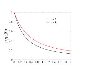
Figure 3: Critical density $\rho_{c}$, normalized by $\rho_{c}(0)$, against the diffusion disorder exponent $c$, for $b=3$ and $b=4$.

4.2 Localization properties of the condensate

It is intuitively clear that the site with the largest single-particle weight ($q_{1}$, say) has the highest chance of hosting the condensate. However, if the spacings between the largest weights $q_{m}$ are small enough, it is plausible to expect a competition amongst the corresponding sites to host the condensate. The aim of this section is to provide a quantitative treatment of this issue.

We first need to characterize the law of spacings between the $q_{m}$. This can be achieved by using the order statistics of the original unordered variables. Let us reorder the sites according to decreasing single-particle weights $q_{m}$ and relabel them so as to have $q_{1}>q_{2}>\dots>q_{M}$. A first estimation of the $m$-th ordered weight $q_{m}$ can be obtained by equating the ratio $m/M$ and the cumulative probability for the random variable $q$ to be larger than $q_{m}$, i.e., $F(q_{m})$, with

$$F(q)=\int_{q}^{1}f(q^{\prime})\,{\rm d}q^{\prime}=(1-q)^{c}.$$ (4.8)

We thus obtain the estimate

$$1-q_{m}\approx\left(\frac{m}{M}\right)^{1/c}.$$ (4.9)

A more precise prediction can be obtained as follows. In the regime of most interest where $M$ is large, while the order $m$ is kept finite, the set of rescaled variables

$$x_{m}=MF(q_{m})=M(1-q_{m})^{c}$$ (4.10)

is asymptotically distributed as Poissonian points with unit density on the positive real line. This property is clear for $c=1$, where the $q_{m}$ are uniformly distributed, so that $F(q)=1-q$. In this case, the variables $x_{m}$ are obtained by ordering $M$ points drawn independently and uniformly in the large interval $[0,M]$. The sequence thus obtained converges to Poissonian points with unit density. The general case then follows by changing variables from $q$ to $1-F(q)$. A full account of the connections between extreme-value statistics or order statistics and point processes can be found in [36, Sec. 7.3].

For Poissonian points with unit density, we have

$$x_{m}=\tau_{1}+\tau_{2}+\cdots+\tau_{m},$$ (4.11)

where the distances $\tau_{m}=x_{m}-x_{m-1}$ between successive points are i.i.d. exponential variables with the distribution $f_{\tau}(\tau)=\rme^{-\tau}$ (and $x_{0}=0$). We thus obtain the more precise estimate

$$1-q_{m}\approx\left(\frac{x_{m}}{M}\right)^{1/c},$$ (4.12)

where the distribution of $x_{m}$ is a Gamma distribution $\Gamma(m,1)$:

$$f_{x_{m}}(x)=\frac{x^{m-1}\,\rme^{-x}}{(m-1)!}.$$ (4.13)

The mean and the variance of $x_{m}$ thus read

$$\overline{x_{m}}=\mathop{\rm var}\nolimits x_{m}=m.$$ (4.14)

So, as the order $m$ gets large, the distribution of $x_{m}$ becomes peaked around $m$, with Gaussian fluctuations of relative order $1/\sqrt{m}$. In this regime (4.12) simplifies to (4.9).

We can now turn to the localization properties of the condensate in the stationary state of a large but finite system. This aspect of the problem is more subtle than the issue discussed in section 4.1. Indeed, a condensate can only be dealt with in the canonical ensemble at fixed $N$, which is less amenable to analytical studies. Moreover, we are interested in properties of single sites ($m=1$, 2, $\dots$) and not in averaged properties over the whole system. We therefore have to rely on the following more heuristic line of reasoning.

Consider a large but finite system in its condensed phase ($M\gg 1$, $\rho>\rho_{c}$), for $b>0$ and for a given draw of the single-particle weights $q_{m}$. We already know the following: in a typical configuration, the condensate is unique, and its size fluctuations around $\Delta=M(\rho-\rho_{c})$ are negligible. Our goal is to estimate the probability $\Pi_{m}$ that site $m$ hosts the condensate in the stationary state. The expression (2.4) of the weight of an arbitrary configuration shows that this probability (unnormalized so far) can be estimated by

$$\Pi_{m}\sim q_{m}^{\Delta},$$ (4.15)

hence, using (4.12),

$$\Pi_{m}\sim\exp\left(-\Delta\left(\frac{x_{m}}{M}\right)^{1/c}\right).$$ (4.16)

The argument of the exponential is proportional to $\Delta/M^{1/c}\sim M^{1-1/c}$. This estimate singles out the borderline value $c=1$, where the dependence on the system size $M$ drops out. This phenomenon already takes place in the simple case of the ZRP on two sites. In this situation, analyzed in A, quantities of interest depend on the rescaled inhomogeneity parameter $\theta=N\varepsilon$ (see (1.5)). In the present case of a large system, the role of $\varepsilon$ is played by the difference between the largest two weights, i.e., $q_{1}-q_{2}\sim M^{-1/c}$ (see (4.12)), so that $\theta\sim\Delta/M^{1/c}\sim M^{1-1/c}$ scales exactly as the argument of the exponential in (4.16).

The following regimes have to be dealt with separately, according to the value of the exponent $c$ with respect to the borderline value $c=1$.

• Extended regime ($c<1$). In this first regime, $\rho_{c}$ is finite for $b>2-c$. The distribution $f(q)$ of the single-particle weights diverges as $q\to q_{\rm max}=1$. Hence the few largest weights $q_{1}$, $q_{2}$, $q_{3},\dots$ pile up near $q=1$. The typical distance between them, scaling as $M^{-1/c}$, is much smaller than the mean spacing $1/M$ in the bulk of the distribution. As a consequence, the probability $\Pi_{m}$ for site $m$ to host the condensate takes appreciable values for many values of $m$. In the regime of interest, i.e., $1\ll m\ll M$, we have $x_{m}\approx m$, and so the estimate (4.16) simplifies to

  $$\Pi_{m} \sim \exp\left(-\Delta\left(\frac{m}{M}\right)^{1/c}\right)$$ (4.17)

  $$\sim \exp\left(-(\rho-\rho_{c})M^{1-1/c}m^{1/c}\right).$$

  The typical number $R$ of favored sites can now be estimated as the range of values of $m$ for which $\Pi_{m}$ remains comparable to $\Pi_{1}$. We are thus led to estimate $R$ as the value of $m$ such that the argument of the exponential function in (4.17) is of order unity. We thus obtain

  $$R\sim\frac{M}{\Delta^{c}}=\frac{M^{1-c}}{(\rho-\rho_{c})^{c}}.$$ (4.18)

  In a typical configuration of the stationary state of the system, there is a unique condensate sitting at a well-defined site. The probabilities $\Pi_{m}$ that the various sites $m$ host the condensate are however extended over a large hosting set of favored sites. The typical size $R$ of this set grows according to the sub-extensive law (4.18). In the $c\to 0$ limit we recover an extensive growth $R\sim M$, in agreement with the fully extended nature of the condensate in the homogeneous ZRP, with its spontaneous symmetry breaking mechanism. In the opposite regime ($c\to 1$), the result (4.18) crosses over to a localized condensate, in agreement with an explicit symmetry breaking mechanism. To sum up, the extended condensed phase, with its sub-extensive hosting set, realizes a continuous interpolation between the two condensation scenarios which were known so far.

• Borderline case ($c=1$). In the borderline situation corresponding to the critical value $c=1$ (and so $\rho_{c}$ is finite for $b>1$), any dependence on the system size drops out of the estimate (4.16), which reads

  $$\Pi_{m}\sim\rme^{-(\rho-\rho_{c})x_{m}},$$ (4.19)

  where the $x_{m}$ are Poissonian points with unit density. The probabilities $\Pi_{m}$ therefore typically take appreciable values on a small and fluctuating number of sites. B is devoted to a detailed study of these fluctuating probabilities. Distributions of this sort seem to have been first described in the context of randomly breaking an interval [37]. They have since then been met in several circumstances. A useful tool to investigate them is provided by the quantity $Y$ (see (2.3)), which is somehow similar to the participation ratio used in the theory of Anderson localization [38]. In the present situation, this quantity $Y$ will be shown to have a non-trivial distribution, which is universal in the sense that it only depends on the parameter $r=\rho-\rho_{c}$.

• Localized regime ($c>1$). For $c>1$ (and so $\rho_{c}$ is now finite for all $b$), the distribution $f(q)$ goes to zero as $q\to q_{\rm max}=1$. The few largest weights $q_{1}$, $q_{2}$, $q_{3},\dots$ are therefore rather distant from one another. The successive distances between them indeed scale as $M^{-1/c}$. As a consequence, for a typical draw of the single-particle weights, the first probability $\Pi_{1}$ is overwhelmingly larger than the other ones. The condensate is therefore localized on the most favored site ($m=1$) with very high probability. The events where the largest two weights $\Pi_{1}$ and $\Pi_{2}$ become comparable occur with a small probability, which can be estimated to be of order $M^{-(1-1/c)}$. These rare events will be analysed more precisely in C.

4.3 Phase diagram

Putting all the above results together, we arrive at the universal phase diagram depicted in figures 1 and 2. The phase diagram shown in figure 1 exhibits three phases in the plane of the exponents $b$ (characterizing interactions) and $c$ (characterizing diffusion disorder). In the fluid phase, there is no condensate at any density. In the localized condensed phase, for $\rho>\rho_{c}$, the condensate lives on the most favored site ($m=1$) with very high probability. In the extended condensed phase, for $\rho>\rho_{c}$, the condensate lives on one of the sites of a large set of favored sites, whose size $R$ grows sub-extensively, according to (4.18). Figure 2 shows a more detailed phase diagram, where the condensed phases are further separated into phases where $\mu_{c}$ is finite, hence the size fluctuations of the condensate around $\Delta$ are normal (i.e., Gaussian and growing as $M^{1/2}$), and phases where $\mu_{c}$ is divergent, hence those fluctuations are anomalous, i.e., not Gaussian and growing faster than $M^{1/2}$. More precisely, these fluctuations scale as $M^{1/c}$ for $b<1$ and $1<c<2$, and as $M^{1/(b+c-1)}$ for $b>1$ and $2-b<c<3-b$. These growth laws can be respectively deduced from the expressions (4.4) and (4.3).

It should be clear from its derivation that the above phase diagram is universal, as announced in the introduction, in the sense that it holds for any rate whose asymptotic behavior at large $k$ is of the form $u_{k}\approx 1+b/k$, hence $P_{\rm sg}(z)\sim(1-z)^{b-1}$, and for any distribution of single-particle weights with a finite maximum $q_{\rm max}$ and a power-law scaling as $f(q)\sim(q_{\rm max}-q)^{c-1}$.

5 Numerical illustrations

This section is devoted to numerical illustrations of the predictions made in the previous section.

5.1 Density and occupation probability profiles

Let us start at a rather qualitative level, and look at the growth of the density profile across a finite system as particles are added one by one. In order to avoid irregularities due to fluctuations, we take the deterministic ordered single-particle weights

$$q_{m}=1-\left(\frac{2m-1}{2M}\right)^{1/c}\qquad(m=1,\dots,M),$$ (5.1)

corresponding to the most uniform non-random sampling of the distribution (1.4).

The left-hand panels of figure 4 show plots of the canonical densities $\rho_{m}=\langle N_{m}\rangle$ of the successive sites ($m=1$, 2, $\dots$), against the mean density $\rho=N/M$ of the system, for $M=50$ and $N$ up to $N_{\rm max}=100$, i.e., $\rho_{\rm max}=2$, for a fixed interaction exponent $b=4$, and the deterministic single-particle weights (5.1) with three values of $c$. The densities $\rho_{m}$ are calculated by means of (2.7)–(2.9). The ordering $q_{1}>q_{2}>q_{3}>\dots$ of the weights always reflects itself into the same ordering for the densities, i.e., $\rho_{1}\hbox{(black)}>\rho_{2}\hbox{(red)}>\rho_{3}\hbox{(green)}>\dots$ The various phases of the system are expected to manifest themselves as different asymptotic growth laws in various parts of the density profile. For $c=0.5$, the densities of the first few sites are observed to grow at similar rates, at least at low enough density. For $c=2$, only the most favored site has a rapidly growing density, whereas all the other densities remain microscopic. Finally, the situation for $c=1$ looks intermediate. These findings are in agreement with the predicted transition at $c=1$ between an extended and a localized condensed phase. Another feature is worth being noticed. As a consequence of the interactions, all the densities $\rho_{m}$ except the first one ($\rho_{1}$) present a maximum for intermediate densities and they eventually decrease at very high mean densities. This phenomenon takes place for any positive values of $b$ and $c$. It is of the same nature as the overshoot observed in the impurity problem [25].

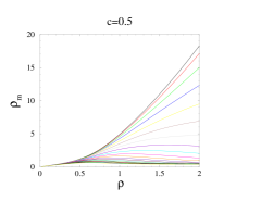
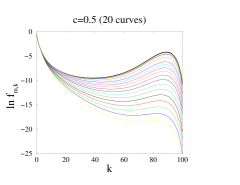
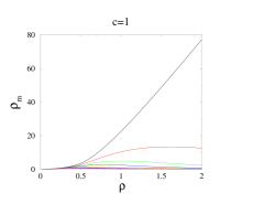
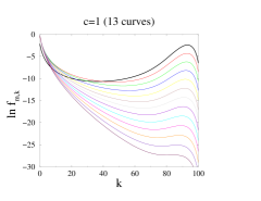
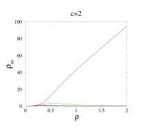
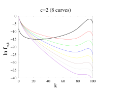
Figure 4: Left: plots of the local densities $\rho_{m}=\langle N_{m}\rangle$ at sites $m=1,2,\dots$ against the mean density $\rho=N/M$, for $M=50$ sites and up to $N_{\rm max}=100$ particles, with $b=4$. Each panel corresponds to a value of $c$. Each color consistently corresponds to a site label (black for $m=1$, red for $m=2$, and so on). Right: logarithmic plots of the occupation probabilities $f_{m,k}$ of the favored sites (see text) against particle number $k$, for $M=50$ and $N=100$. Other parameters and colors are the same as for the left-hand panels.

The right-hand panels of figure 4 show logarithmic plots of the local occupation probabilities $f_{m,k}$ of the successive sites ($m=1$, 2, $\dots$), against $k$, for the same model parameters with $N=100$ particles on $M=50$ sites. These occupation probabilities are calculated by means of (2.8). The favored sites, corresponding to the smaller values of $m$, present a non-monotonic profile of occupation probabilities, with a local minimum at $k_{\rm min}\approx\Delta/2$, and a secondary peak at $k_{\rm max}\approx\Delta$, representing the condensate. Only the data for those favored sites have been plotted for clarity. The numbers of curves (20, 13, and 8) therefore give the numbers of those favored sites. For a given favored site $m$, the area under the secondary peak,

$$\Pi_{m}=\sum_{k=k_{\rm min}}^{N}f_{m,k},$$ (5.2)

gives an operational estimate of the hosting probability of site $m$. As $c$ increases, the number of favored sites decreases, and the hosting probabilities $\Pi_{m}$ decrease more and more rapidly (remember the vertical scale on the right-hand panels of figure 4 is logarithmic).

The role of the disorder exponent $c$ is further emphasized in figure 5, showing an enlargement of the first two datasets presented on the right-hand side of figure 4, in the region of the condensate peak and on a linear scale. The contrast between the two situations corroborates our prediction. For $c=0.5$ (in the extended phase), a large number of favored sites exhibit a visible secondary peak, and thus host the condensate with an appreciable probability. For $c=1$ (at the borderline between the extended and localized phases), only a small number of sites (4 on the plot) exhibit a visible secondary peak, and the areas under the peaks decrease very rapidly. In both cases the maxima of the peaks roughly coincide with the predictions $k=\Delta=N-M\rho_{c}$, i.e., $k=87$ for $c=0.5$ ($\rho_{c}=0.2555$) and $k=92$ for $c=1$ ($\rho_{c}=0.1641$) (vertical dashed lines).

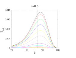
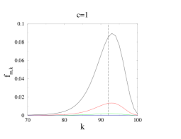
Figure 5: Enlargement of first two datasets presented on the right-hand side of figure 4, in the region of the condensate peak and on a linear scale. Vertical dashed lines: thermodynamic predictions for the mean condensate size $\Delta$.

5.2 A quantitative study of the hosting probabilities

We now turn to the most novel prediction of this work, namely the existence of an extended condensed phase, where the condensate can be hosted by a large set of favored sites, whose size $R$ obeys the sub-extensive growth law (4.18).

Let us first examine the individual hosting probabilities $\Pi_{m}$. Considering $c=0.5$ for definiteness, the estimate (4.17) simplifies to the half-Gaussian law

$$\Pi_{m}\sim\exp\left(-\frac{(\rho-\rho_{c})m^{2}}{M}\right).$$ (5.3)

Figure 6 shows a logarithmic plot of the hosting probabilities, calculated by means of (2.7), (2.8), and (5.2), for all the sites $m$ having a condensate peak, against $m^{2}/M$, for $b=4$ and $\rho=2$, in three situations: a random sample of $M=100$ sites, a random sample of $M=200$ sites, and a deterministic sample of $M=200$ sites with single-particle weights (5.1). The black line with slope $\rho-\rho_{c}=1.7445$ shows the theoretical estimate (5.3). The dataset of the deterministic sample is found to accurately follow the theoretical slope. The data for the two random samples exhibit the expected trend, although they are too noisy to be conclusive. This observation justifies our choice to use deterministic single-particle weights as illustrative examples in figures 4 and 5. Finally, it is worth noticing that the sum of all the hosting probabilities,

$$S_{1}=\sum_{m=1}^{M}\Pi_{m},$$ (5.4)

is very close to unity in the three situations shown in figure 6. We indeed respectively find $S_{1}-1=7.92\times 10^{-6}$, $4.73\times 10^{-6}$, and $4.42\times 10^{-6}$. The asymptotic sum rule $S_{1}=1$, testifying the uniqueness of the condensate in the thermodynamic limit, is therefore verified with high accuracy for system sizes as small as $M=100$.

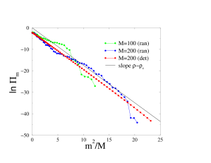
Figure 6: Logarithmic plot of the hosting probabilities $\Pi_{m}$ against $m^{2}/M$, for $b=4$, $c=1/2$ and $\rho=2$ in three cases (see text). Black line with slope $\rho-\rho_{c}=1.7445$: theoretical estimate (5.3).

We proceed by an investigation of the size $R$ of the hosting set for the condensate. Along the lines of the theory of Anderson localization [38], we can expect that a reliable estimate of $R$ will be provided by the inverse participation ratio,

$$R=\displaystyle{\frac{\displaystyle\left(\sum_{m=1}^{M}\Pi_{m}\right)^{2}}{\displaystyle\sum_{m=1}^{M}\Pi_{m}^{2}}},$$ (5.5)

i.e., the inverse of the quantity $Y$ defined in (2.3). This operational definition holds for any finite sample. The hosting probability $\Pi_{m}$ of a favored site $m$ is measured as the area under the condensate peak (see (5.2)), and set to zero for the unfavored sites where the occupation probabilities $f_{m,k}$ exhibit no such peak. The normalization in the numerator of (5.5) is needed for the smaller systems, where the $\Pi_{m}$ do not exactly sum up to unity. We now have a tool to help us revisiting the various regimes of the phase diagram.

• Extended regime ($c<1$). In this regime, it is legitimate to make use of the expression (4.17) for the hosting probabilities $\Pi_{m}$ in order to estimate the quantity $R$ defined in (5.5). Evaluating the sums as integrals, we end up with the result that $R$ is asymptotically self-averaging and grows as

  $$R\approx A\,M^{1-c},\qquad A=\left(\frac{2}{\rho-\rho_{c}}\right)^{c}\Gamma(c+1).$$ (5.6)

  The scaling estimate (4.18) has thus been turned into a quantitative prediction. Figure 7 shows plots of the mean size $\overline{R}$ of the hosting set, for $\rho=2$ and $b=3$ and $b=4$, against $M^{1/2}$ for $c=0.5$ (left) and against $M^{1/4}$ for $c=0.75$ (right). All the data presented in figures 7–9 have been obtained by generating many (typically $10^{5}$) independent configurations of $M$ single-particle weights $\{q_{m}\}$ drawn from the distribution (1.4), and by exactly evaluating for each configuration the quantity $R$ by means of (2.7), (2.8), (5.2), and (5.5). All the datasets shown in figure 7 exhibit a linear behavior, corroborating the power-law growth (5.6), and show a reasonable quantitative agreement with the predicted amplitudes $A$.

  

  

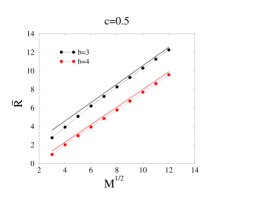
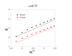
  Figure 7: Mean size $\overline{R}$ of the hosting set in the extended regime. Straight lines have the theoretical slopes $A$ (see (5.6)). Left: Data for $c=0.5$ and $\rho=2$ against $M^{1/2}$. For $b=3$, $\rho_{c}=0.4140$ and $A=0.9952$. For $b=4$ (data shifted vertically for readability), $\rho_{c}=0.2555$ and $A=0.9489$. Right: Data for $c=0.75$ and $\rho=2$ against $M^{1/4}$. For $b=3$, $\rho_{c}=0.3078$ and $A=1.0418$. For $b=4$ (data shifted vertically for readability), $\rho_{c}=0.2007$ and $A=0.9949$.

• Borderline case ($c=1$). This borderline situation is investigated in detail in B. The quantity $R$, which identifies with $1/Y$ (see (2.3)), has a non-trivial limit distribution which only depends on $r=\rho-\rho_{c}$. An expression for the mean value $\overline{R}$ is given in (2.31). Figure 8 shows a plot of $\overline{R}$ against $M$ for $\rho=2$ and $b=3$ and $b=4$. The data seem to exhibit a fast convergence to well-defined limits. The apparent limiting values however show a slight disagreement (of the order of half a percent in relative value) with the theoretical predictions given in (2.31) (horizontal lines), i.e., $\overline{R}=1.9411$ for $b=3$ ($\rho_{c}=0.2421$, $r=1.7579$), and $\overline{R}=1.8995$ for $b=4$ ($\rho_{c}=0.1641$, $r=1.8359$). The observed discrepancy is most certainly attributable to a very slow convergence. The data (not presented here) with the deterministic sampling (5.1) indeed exhibit a similar slow convergence, albeit toward different limiting values.

  

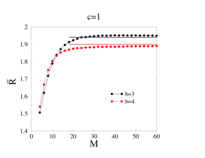
  Figure 8: Mean size $\overline{R}$ of the hosting set in the borderline case ($c=1$) against $M$, for $\rho=2$ and $b=3$ and $b=4$. Horizontal lines: predicted limiting values $\overline{R}=1.9411$ for $b=3$ ($\rho_{c}=0.2421$, $r=1.7579$), $\overline{R}=1.8995$ for $b=4$ ($\rho_{c}=0.1641$, $r=1.8359$) (see (2.31)).

• Localized regime ($c>1$). In this regime, we argued in section 4 that the condensate is localized on the most favored site ($m=1$) with very high probability, hence $R$ should converge to unity for large systems. The first correction to this trivial limit comes from the rare events where the weights $\Pi_{1}$ and $\Pi_{2}$ are comparable. The probability for this to occur falls off as $1/M^{1-1/c}$. In C this argument is turned into the quantitative prediction (see (3.7))

  $$\overline{R}-1\approx\frac{\pi c\,\Gamma(2-1/c)}{2(\rho-\rho_{c})}\,M^{-(1-1/c)}.$$ (5.7)

  For $c=2$ this yields

  $$\overline{R}-1\approx\frac{\pi^{3/2}}{2(\rho-\rho_{c})\sqrt{M}}.$$ (5.8)

  Figure 9 shows a plot of $\overline{R}$ against $M$ for $b=4$ and $c=2$ (and so $\rho_{c}=0.0927$), and $\rho=2$. The data exhibit a smooth maximum near $\overline{R}\approx 1.39$ for $M=7$, whereas they slowly go to unity for large systems, in good agreement with the theoretical prediction (5.8), i.e., $\overline{R}\approx 1+1.4597/\sqrt{M}$.

  

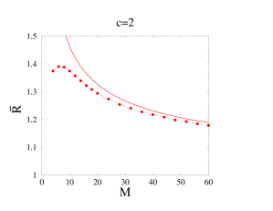
  Figure 9: Mean size $\overline{R}$ of the hosting set in the localized regime ($c=2$) against $M$ for $b=4$ (and so $\rho_{c}=0.0927$), and $\rho=2$. Full red line: theoretical prediction (5.8), i.e., $\overline{R}\approx 1+1.4597/\sqrt{M}$.

6 Complex networks

In this section we investigate to what extent the above results concerning localization properties of the condensate apply to the ZRP on complex networks [39]. These networks are usually scale-free, i.e., characterized by a broad distribution of the node degrees $K_{m}$, falling off as the power law $f_{K}\sim K^{-\gamma}$, with $\gamma>2$.

In the simplest situation where individual particles perform ordinary random walk, the stationary weight $q_{m}$ at node $m$ is proportional to the degree $K_{m}$. The ZRP with this underlying inhomogeneous diffusion has been investigated by several groups [27, 28, 29]. Strictly speaking, this situation does not fit within the present work, as node degrees are unbounded. In other words, we have $q_{\rm max}=\infty$ and $z_{c}=0$, and so the model does not have a fluid grand-canonical phase. It has indeed been shown [27] that this inhomogeneous ZRP exhibits complete condensation (at least when $u_{k}=1$), in the (weak) sense that the critical density $\rho_{c}$ vanishes in the thermodynamic limit.

Consider a large but finite network consisting of $M$ nodes. We have thus approximately $\Delta\approx N=M\rho$. The nodes which can host the condensate are those with highest degrees, whose statistics has been studied recently [40, 41]. The node whose degree $K_{1}$ is the highest is called the leader in those references. The estimate $K_{1}\sim M^{1/(\gamma-1)}$ is easily obtained from an argument of extreme-value statistics. Two situations have to be dealt with separately.

• There is a single leader, i.e., a single node with highest degree $K_{1}$. In that case, we have $K_{2}=K_{1}-j$ for some $j=1,2,\dots$ and so $-\ln(\Pi_{2}/\Pi_{1})\approx j\Delta/K_{1}\sim M^{(\gamma-2)/(\gamma-1)}$. The hosting probability $\Pi_{2}$ is therefore exponentially small. The condensate is therefore hosted by the unique leader with an overwhelmingly high probability.

• There are more than one node with highest degree $K_{1}$. Let $C=2$, 3, $\dots$ denote the number of these co-leaders. In that case, the condensate is hosted by each co-leader with equal probability, and so we have $R=C$. It has been shown in [41] that the probability of having $C$ co-leaders decreases rapidly with $C$, and that the leading event, namely the presence of two co-leaders ($C=2$), occurs with a probability of the order of $1/K_{1}$. We thus obtain the estimate

  $$\overline{R}-1\sim M^{-1/(\gamma-1)}.$$ (6.1)

There is a striking similarity between this result and the prediction (5.7) in the localized regime ($c>1$). The ZRP with inhomogeneous diffusion on complex networks is therefore always in the localized regime. The quantitative correspondence between exponents reads

$$c=\frac{\gamma-1}{\gamma-2},\qquad\mbox{i.e.,}\quad\gamma=\frac{2c-1}{c-1}.$$ (6.2)

The predictions made here are entirely due to the possible existence of co-leaders.

7 Discussion

In this work we have investigated the combined effects of interactions and diffusion disorder on the condensation phenomenon in the inhomogeneous ZRP. Our main findings have been summarized in the phase diagrams shown in figures 1 and 2. These universal phase diagrams are drawn in the plane of two exponents, the interaction exponent $b$ of the rate (1.5) and the disorder exponent $c$ of the distribution (1.4) of the single-particle weights modeling inhomogeneous diffusion.

The most prominent feature put forward in this work is the existence of an extended condensed phase. This novel phase, which corresponds to the domain where $0<c<1$ and $b>2-c$, therefore shows up as a result of the combined effects of strong enough interaction and weak enough disorder. In this phase, a typical high-density configuration has a unique condensate on top of a critical background, but the condensate may be located at any site of a large hosting set of favored sites, whose size grows sub-extensively as $R\sim M^{1-c}$. The extended condensed phase can therefore be viewed as implementing a continuous interpolation between the two symmetry breaking scenarios known so far, namely SSB in the homogeneous ZRP and ESB in the occupation-independent inhomogeneous case.

It is worth underlining the qualitative difference between the extended condensed phase of the inhomogeneous ZRP emphasized in this work and several alternative condensation scenarios in interacting particle systems which have been put forward in the recent literature. The homogeneous ZRP with non-conventional hopping rates $u_{k}$, exhibiting either a non-monotonic dependence on the occupation $k$ or a weak explicit dependence on the system size, may have several ‘condensates’ in its stationary state [42, 43]. These new scenarios include the possibility of having an extensive number of ‘condensates’ whose typical size is finite but parametrically large, or a sub-extensive number of ‘meso-condensates’, each of them having typically a sub-extensive population. Some mass transport models, where the hopping rate (generalizing $u_{k}$) also depends on the occupation of neighboring sites, have been shown to develop an extended condensate, i.e., a high-density structure containing all the excess particles and extending over a number of sites of order $M^{1/2}$ [44]. The non-universal properties of the extended condensate in this class of models have been underlined in [45]. Another variant of these models in one dimension leads to a phenomenon of explosive condensation, giving rise to a moving condensate sweeping the system at an accelerated pace [46]. The ‘target process’, introduced in [47], is dual to the ZRP, in the sense that the hopping rate now depends on the occupation of the arrival site. In the case of asymmetric dynamics in two dimensions and above, the stationary state again contains a one-dimensional extended condensate, aligned with the direction of the mean current. The ‘inclusion process’, where particles are allowed to make non-local jumps over the lattice, exhibits unusual types of complete condensation, including a case where almost all the particles are condensed on the right-most side of a finite one-dimensional chain [48]. Finally, a non-Markovian generalization of the ZRP, where the motion of particles is governed by internal clocks endowed with their own dynamics, leads to a variety of non-equilibrium stationary states. In the asymmetric one-dimensional situation, the model may exhibit a localized condensate sitting on two neighboring sites and moving ballistically [49].

The present work focussed on the stationary state of the ZRP with inhomogeneous diffusion (1.4) and interaction (1.5). The dynamical consequences of our findings are clearly the next question of interest. For the case of homogeneous diffusion on a large but finite system, the ergodic motion of the condensate in the stationary state has been investigated by the present authors in [14]. The leading mechanism turns out to be that all the excess particles sequentially quit the condensate and progressively rebuild it at another random distant site. The associated characteristic time scale can therefore be analyzed by means of an effective two-site model, with the key ingredient being the occupation probability profile $f_{k}$ of the latter model. This ergodic time scale is found to grow with the system size as the power law

$$\tau\sim\frac{\Delta^{b+1}}{M}\sim M^{b},$$ (7.1)

i.e., faster than the diffusive scale $M^{2}$ in the thermodynamic limit (as $b>2$), but not exponentially fast. (In the special situation of symmetric dynamics in one dimension, our prediction is increased to $\tau\sim\Delta^{b+1}$.) The scaling prediction (7.1) has been alluded to or used in several situations germane to the present one [28, 42, 43, 46, 47, 48, 49]. It has also been corroborated by a recent rigorous analysis [19], albeit in the regime where $N$ becomes large while $M$ is kept finite. Coming back to the inhomogeneous ZRP studied in the present work, the occupation probability profile on two sites exhibits a universal ‘dip’, scaling as $N^{-b}$, irrespective of the inhomogeneity (see (1.17)). It can therefore be expected that the scaling law (7.1) will still hold all over the extended condensed phase of the model (for $b>2$), where the condensate is allowed to live on a large hosting set of favored sites. In the region of the phase diagram where $2-c<b<2$ the ergodic time should scale as the diffusive one. Finally the coarsening process of the formation of the condensate is yet another facet of the dynamics worth investigating.

Acknowledgments

It is a pleasure to thank Stefan Grosskinsky for interesting discussions.

Appendix A The case of two sites

Let us consider the simplest non-trivial situation of the inhomogeneous ZRP on two sites. The quantities of interest can be given explicit expressions in this situation, while its behavior is already illustrative of many features of the model on larger systems.

The single-particle weights $q_{1}$ and $q_{2}$ and the hopping rates $w_{12}$ and $w_{21}$ are related by $w_{12}q_{1}=w_{21}q_{2}$ (see (1.1)). We introduce an inhomogeneity parameter $\varepsilon$ so that $q_{1}/q_{2}=w_{21}/w_{12}=\rme^{2\varepsilon}$, and parametrize the single-particle weights as

$$q_{1}=\rme^{\varepsilon},\qquad q_{2}=\rme^{-\varepsilon}.$$ (1.1)

For definiteness, we set $\varepsilon>0$, so that $q_{1}>q_{2}$, i.e., site 1 is favored.

A.1 The occupation-independent case ($u_{k}=1$)

Let us start with the occupation-independent case ($u_{k}=1$), and consider the canonical ensemble where the total number $N$ of particles is fixed.

The partition function (2.36) becomes

$$Z_{2,N}=\frac{q_{1}^{N+1}-q_{2}^{N+1}}{q_{1}-q_{2}}=\frac{\sinh(N+1)\varepsilon}{\sinh\varepsilon}.$$ (1.2)

Setting $N_{1}=k$ and $N_{2}=N-k$, the occupation probabilities read

$$f_{k}=\mathop{\rm Prob}\nolimits\{N_{1}=k\}=\frac{q_{1}^{k}q_{2}^{N-k}}{Z_{2,N}}=\frac{\sinh\varepsilon\,\rme^{(2k-N)\varepsilon}}{\sinh(N+1)\varepsilon}.$$ (1.3)

The occupation probability profile is thus exponentially increasing from the least probable event (site 1 is empty, i.e., $k=0$) to the most probable one (site 2 is empty, i.e., $k=N$). The ratio between the smallest and the largest of these probabilities reads

$$\frac{f_{0}}{f_{N}}=\left(\frac{q_{2}}{q_{1}}\right)^{N}=\rme^{-2N\varepsilon}.$$ (1.4)

When the number of particles $N$ becomes large, in order for the populations of the two sites to remain comparable, one has to keep the model in the regime of a weak inhomogeneity, where $\varepsilon$ scales as $1/N$. In this regime, many results assume scaling forms, involving the rescaled inhomogeneity parameter

$$\theta=N\varepsilon.$$ (1.5)

For instance, the normalized occupation probability profile becomes

$$f_{k}\approx\frac{\varepsilon\,\rme^{(2x-1)\theta}}{\sinh\theta}\qquad(0<x=k/N<1)$$ (1.6)

and, in particular, the probability ratio (1.4) becomes $\rme^{-2\theta}$. The density contrast

$$\delta\rho=\rho_{1}-\rho_{2}=\langle N_{1}-N_{2}\rangle=\frac{\partial}{\partial\varepsilon}\ln Z_{2,N}$$ (1.7)

scales as

$$\delta\rho\approx N\,\Phi_{0}(\theta),$$ (1.8)

where the scaling function

$$\Phi_{0}(\theta)=\mathop{\rm cotanh}\nolimits\theta-\frac{1}{\theta}$$ (1.9)

starts increasing linearly as $\Phi_{0}(\theta)\approx\theta/3$ for small $\theta$, and slowly saturates to unity as $\Phi_{0}(\theta)\approx 1-1/\theta$ at large $\theta$.

Let us briefly consider the grand-canonical case. We have (see (2.31))

$$\rho^{{\rm GC}}_{1}=\frac{z\rme^{\varepsilon}}{1-z\rme^{\varepsilon}},\qquad\rho^{{\rm GC}}_{2}=\frac{z\rme^{-\varepsilon}}{1-z\rme^{-\varepsilon}}.$$ (1.10)

The fugacity $z$ is determined by imposing the mean total occupation $\langle N^{{\rm GC}}\rangle=\rho^{{\rm GC}}_{1}+\rho^{{\rm GC}}_{2}$. Skipping details, we again find that the density contrast $\delta\rho^{{\rm GC}}=\rho^{{\rm GC}}_{1}-\rho^{{\rm GC}}_{2}$ obeys a scaling law of the form (1.9), with $\theta=\langle N^{{\rm GC}}\rangle\varepsilon$ and

$$\Phi^{{\rm GC}}_{0}(\theta)=\frac{\theta}{1+\sqrt{\theta^{2}+1}}.$$ (1.11)

This scaling function is rather close to its canonical counterpart (1.9). It starts increasing as $\Phi^{{\rm GC}}_{0}(\theta)\approx\theta/2$ and slowly saturates to unity as $\Phi^{{\rm GC}}_{0}(\theta)\approx 1-1/\theta$. Both functions will be plotted in figure 11.

A.2 The general case

We now turn to the general case of the inhomogeneous ZRP on two sites with the rate (1.5), considering only the canonical ensemble and keeping the same notations as above.

The occupation probabilities read

$$f_{k}=\mathop{\rm Prob}\nolimits\{N_{1}=k\}=\frac{\rme^{(2k-N)\varepsilon}p_{k}p_{N-k}}{Z_{2,N}},$$ (1.12)

where the partition function is

$$Z_{2,N}=\sum_{k=0}^{N}\rme^{(2k-N)\varepsilon}p_{k}p_{N-k}.$$ (1.13)

In the presence of attractive interactions, i.e., for $b>0$, the most probable event is still that site 2 is empty (i.e., $k=N$), and the result (1.4) still holds. More interestingly, however, the occupation probability profile approximately reads

$$f_{k}\approx\frac{\Gamma(b+1)^{2}}{Z_{2,N}}\,\frac{\rme^{(2k-N)\varepsilon}}{k^{b}(N-k)^{b}},$$ (1.14)

whenever both populations are large (i.e., $k\gg 1$ and $N-k\gg 1$). The above expression is the product of an increasing exponential (reflecting the inhomogeneity) and of two decaying power laws (reflecting the attractive interactions).

In the scaling regime of a weak inhomogeneity ($N$ large, $\varepsilon$ small, $\theta=N\varepsilon$ fixed), the above probability profile has a deep minimum for a non-trivial value $k_{\rm min}$ of the occupation $k$, namely

$$k_{\rm min}\approx A(\theta)\,\frac{N}{2},$$ (1.15)

with

$$A(\theta)=\frac{2b}{b+\theta+\sqrt{b^{2}+\theta^{2}}}.$$ (1.16)

The corresponding smallest probability scales as

$$\frac{f_{\rm min}}{\sqrt{f_{0}f_{N}}}\approx B(\theta)\,2^{2b}\,\Gamma(b+1)\,N^{-b},$$ (1.17)

with

$$B(\theta)=\left(\frac{b+\sqrt{b^{2}+\theta^{2}}}{2b}\right)^{b}.$$ (1.18)

The probability profile therefore exhibits a universal dip, in the language of [14], whose scaling in $N^{-b}$ holds irrespectively of the rescaled inhomogeneity parameter $\theta$, which only enters the scaling functions $A(\theta)$ and $B(\theta)$. These functions are normalized so that $A(0)=B(0)=1$ in the homogeneous limit. The occurrence of a universal dip in the occupation probability profile is the gist of the uniqueness of the condensate in the inhomogeneous ZRP for any $b>0$. It also has far-reaching dynamical consequences, which are briefly discussed in section 7. Figure 10 shows a logarithmic plot of the occupation probabilities $f_{k}$ for $N=100$ particles on two sites, for $b=1$ and several values of $\theta$.

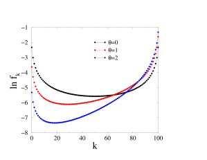
Figure 10: Logarithmic plot of the occupation probabilities $f_{k}$ for $N=100$ particles on two sites, with $b=1$ and several values of $\theta$.

In order to derive more quantitative predictions concerning the scaling behavior of the partition function $Z_{2,N}$ and of the density contrast $\delta\rho$, the following two regimes have to be considered separately, along the lines of [14].

• For $b>1$, the sum in (1.13) is dominated by configurations such that almost all the particles sit on one site, i.e., either $k$ is finite, or $N-k$ is finite. Indeed the sum $P(1)$ of the $p_{k}$ is convergent (see (3.6)). In other words, there is complete condensation in the $N\to\infty$ limit.

  We thus obtain in the scaling regime

  $$Z_{2,N}\approx\frac{2b\Gamma(b+1)}{b-1}\,N^{-b}\,\cosh\theta$$ (1.19)

  and

  $$\delta\rho\approx N\,\Phi_{1}(\theta),$$ (1.20)

  where

  $$\Phi_{1}(\theta)=\tanh\theta$$ (1.21)

  is independent of $b$ in the range $b>1$. The above scaling function starts linearly as $\Phi_{1}(\theta)\approx\theta$ and saturates exponentially fast to unity as $\Phi_{1}(\theta)\approx 1-2\rme^{-\theta}$.

• For $b<1$, the sum of the $p_{k}$ is divergent, and so all values of $k$ contribute to the sum in (1.13). Evaluating this sum in the scaling regime as an integral over $y=2x-1=2k/N-1$, we obtain

  $$Z_{2,N}\approx\frac{(\pi b)^{2}}{\Gamma(2-2b)\,\sin^{2}(\pi b)}N^{1-2b}\,F_{b}(\theta),$$ (1.22)

  with

  $$F_{b}(\theta) = \frac{\Gamma(3/2-b)}{\sqrt{\pi}\,\Gamma(1-b)}\int_{-1}^{+1}\frac{\rme^{\theta y}\,{\rm d}y}{(1-y^{2})^{b}}$$ (1.23)

  $$= \Gamma(3/2-b)(\theta/2)^{b-1/2}I_{1/2-b}(\theta),$$

  where $I_{\nu}(\theta)$ denotes the modified Bessel function of index $\nu$. The above scaling function is again normalized so that $F_{b}(0)=1$ in the homogeneous limit. We thus have

  $$\delta\rho\approx N\,\Phi_{b}(\theta),$$ (1.24)

  with

  $$\Phi_{b}(\theta)=\frac{F^{\prime}_{b}(\theta)}{F_{b}(\theta)}=\frac{I_{3/2-b}(\theta)}{I_{1/2-b}(\theta)}.$$ (1.25)

  This scaling function starts linearly as $\Phi_{b}(\theta)\approx\theta/(3-2b)$ and slowly saturates to unity as $\Phi_{b}(\theta)\approx 1-(1-b)/\theta$. The result (1.9) is recovered for $b=0$.

  The function $\Phi_{b}(\theta)$ coincides with the function describing Langevin paramagnetism in dimension $d=3-2b$. Indeed, setting $y=\cos u$, the integral (1.23) can be recast as

  $$F_{b}(\theta)=\frac{\Gamma(d/2)}{\sqrt{\pi}\,\Gamma((d-1)/2)}\int_{0}^{\pi}(\sin u)^{d-2}\rme^{\theta\cos u}\,{\rm d}u,$$ (1.26)

  where we recognize the normalized partition function for a classical spin, represented by a vector ${\bf s}$ describing the unit sphere in $d$ dimensions, coupled to a reduced magnetic field $\theta$, so that $u$ is the angle between ${\bf s}$ and the direction of the field. This analogy makes sense as long as ${\bf s}$ has continuous degrees of freedom, namely for $d>1$, i.e., precisely $b<1$.

Figure 11 shows the scaling function $\Phi_{b}$ of the density contrast for several $b$. This function is independent of $b$ and saturates exponentially fast for $b>1$, whereas it depends continuously on $b$ and saturates slowly for $b<1$. Furthermore, at least for the case $b=0$, the grand-canonical scaling function is very close to its canonical counterpart.

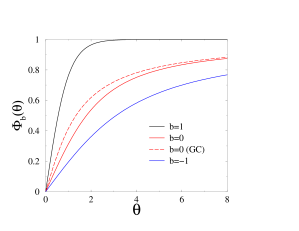
Figure 11: Finite-size scaling functions $\Phi_{b}(\theta)$ describing the density contrast of the two-site problem, against the rescaled inhomogeneity parameter $\theta$, for various values of the exponent $b$. The grand-canonical scaling function $\Phi^{{\rm GC}}_{0}(\theta)$ is also plotted for comparison.

Appendix B Universal fluctuations in the borderline situation ($c=1$)

This Appendix is devoted to a detailed study of the fluctuations of the hosting probabilities $\Pi_{m}$ of a large system in the borderline situation ($c=1$). We are thus led to consider an infinite ordered sequence of unnormalized weights of the form (see (4.19))

$$\Pi_{m}=\rme^{-rx_{m}}\qquad(m=1,2,\dots),$$ (2.1)

where the $x_{m}$ are Poissonian points with unit density, whereas $r=\rho-\rho_{c}$ is the control parameter of the problem.

We are interested in the joint distribution of the two sums

$$S_{1}=\sum_{m\geq 1}\Pi_{m},\qquad S_{2}=\sum_{m\geq 1}\Pi_{m}^{2},$$ (2.2)

and chiefly in the distribution of the ratio

$$Y=\frac{S_{2}}{S_{1}^{2}},$$ (2.3)

introduced in [37].

The formula (4.11) allows us to recast the definition of the sums $S_{1}$ and $S_{2}$ into the form

$$S_{1} = X_{1}+X_{1}X_{2}+X_{1}X_{2}X_{3}+\cdots,$$

$$S_{2} = X_{1}^{2}+X_{1}^{2}X_{2}^{2}+X_{1}^{2}X_{2}^{2}X_{3}^{2}+\cdots,$$ (2.4)

where the $X_{m}=\rme^{-r\tau_{m}}$ are i.i.d. random variables with the distribution

$$f_{X}(X)=\frac{1}{r}X^{-1+1/r}\qquad(0<X<1).$$ (2.5)

Infinite random sums such as (2.4) are known as Kesten variables [50, 51]. They have been shown to play a role in various areas of the physics of one-dimensional disordered systems [52, 53, 54]. In the present situation, we have the identities

$$S_{1}\equiv X(1+S_{1}^{\prime}),\qquad S_{2}\equiv X^{2}(1+S_{2}^{\prime}),$$ (2.6)

where $X$ is drawn from the distribution (2.5) and $S_{1}^{\prime}$ and $S_{2}^{\prime}$ are copies of the variables $S_{1}$ and $S_{2}$, independent of $X$. The above identities can be viewed as a stochastic dynamical system for two degrees of freedom, described by the coupled variables $S_{1}$ and $S_{2}$, and submitted to the same noise $X$.

B.1 Distribution of the normalization sum $S_{1}$

The distribution of a Kesten variable such as $S_{1}$ can only be worked out for special distributions of the $X_{m}$ [53]. The present situation, where the $X_{m}$ have a power-law distribution on the interval $[0,1]$, is the simplest of all the exactly solvable cases [51]. It is convenient to use the Laplace transform of the distribution,

$$L_{1}(t)=\overline{\rme^{-tS_{1}}}.$$ (2.7)

The identity (2.6) for $S_{1}$ yields

$$L_{1}(t)=\overline{\rme^{-tX(1+S_{1}^{\prime})}}=\int_{0}^{1}f_{X}(X)\,\rme^{-tX}\,L_{1}(tX)\,{\rm d}X.$$ (2.8)

The change of variable from $X$ to $u=tX$ leads to

$$L_{1}(t)=\frac{1}{r}\,t^{-1/r}\int_{0}^{t}u^{-1+1/r}\,\rme^{-u}\,L_{1}(u)\,{\rm d}u,$$ (2.9)

hence the differential equation

$$L_{1}^{\prime}(t)=-\frac{1-\rme^{-t}}{rt}\,L_{1}(t)$$ (2.10)

and the explicit expression

$$L_{1}(t)=\rme^{-F_{1}(t)/r},$$ (2.11)

with

$$F_{1}(t) = \int_{0}^{1}(1-\rme^{-tx})\frac{{\rm d}x}{x}$$ (2.12)

$$= \int_{0}^{t}\frac{1-\rme^{-u}}{u}\,{\rm d}u=\ln t+\gamma-{\rm Ei}(-t)=\sum_{n\geq 1}\frac{(-1)^{n-1}t^{n}}{n\,n!},$$

where $\gamma=0.577\,215\dots$ denotes Euler’s constant, and Ei is the exponential integral.

The series in the rightmost side of (2.12) demonstrates that the cumulants of $S_{1}$ have the simple expression

$${\overline{S_{1}^{n}}}^{({\rm c})}=\frac{1}{nr}.$$ (2.13)

We have in particular $\overline{S_{1}}=1/r$ and $\mathop{\rm var}\nolimits S_{1}=1/(2r)$, and so $1/r$ can be interpreted as the effective number of significant weights which contribute to the sums (2.2).

The full distribution of $S_{1}$ reads

$$f_{S_{1}}(S_{1})=\int\frac{{\rm d}t}{2\pi{\rm i}}\,\rme^{tS_{1}-F_{1}(t)/r}.$$ (2.14)

Figure 12 shows a plot of this distribution for three characteristic values of the control parameter $r$. Each dataset consisting of 200 bins has been obtained by means of $10^{9}$ iterations of the random recursion (2.6).

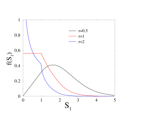
Figure 12: Distribution $f_{S_{1}}(S_{1})$ of the normalization sum $S_{1}$, for three characteristic values of the control parameter $r$.

The distribution $f_{S_{1}}$ becomes a narrow Gaussian in the $r\to 0$ limit, in qualitative agreement with the law of large numbers, as the number $1/r$ of significant weights is large. It gets progressively broader as $r$ increases.

The behavior of $f_{S_{1}}$ for small values of $S_{1}$ can be estimated by using large positive values of $t$ in the contour integral (2.14). Neglecting the exponentially small function ${\rm Ei}(-t)$, we readily obtain the power law

$$f_{S_{1}}(S_{1})\approx\frac{\rme^{-\gamma/r}}{\Gamma(1/r)}\,S_{1}^{-1+1/r}\qquad(S_{1}\to 0).$$ (2.15)

The density therefore diverges as $S_{1}\to 0$ for $r>1$, whereas it tends to zero for $r<1$. This feature is clearly visible on figure 12: $f_{S_{1}}$ vanishes linearly for $r=1/2$, goes to the constant $\rme^{-\gamma}$ for $r=1$, and diverge as $1/\sqrt{S_{1}}$ for $r=2$.

The behaviour of $f_{S_{1}}(S_{1})$ for large values of $S_{1}$ can be estimated from the contour integral (2.14) by means of the saddle-point method. Skipping details, we are left with a super-exponential tail of the form

$$f_{S_{1}}(S_{1})\sim\exp\Bigl{(}-S_{1}(\ln S_{1}+\ln(\ln S_{1})+\ln r+\cdots)\Bigr{)}.$$ (2.16)

Finally, performing an integration by parts in (2.14), we obtain the following differential-difference equation for the distribution $f_{S_{1}}(S_{1})$:

$$(r-1)f_{S_{1}}(S_{1})+rS_{1}f_{S_{1}}^{\prime}(S_{1})+f_{S_{1}}(S_{1}-1)=0.$$ (2.17)

This functional equation has many consequences, including that the estimate (2.15) holds identically over the interval $0<S_{1}<1$, and that the distribution $f_{S_{1}}(S_{1})$ has weaker and weaker singularities at all the integer values $S_{1}=1,2,\dots$ Distributions of this kind have been met in several instances, starting with Rényi’s analysis of the one-dimensional car parking problem [55].

B.2 Joint distribution of the sums $S_{1}$ and $S_{2}$

The joint distribution $f_{S_{1},S_{2}}(S_{1},S_{2})$ of the sums $S_{1}$ and $S_{2}$ can be studied along the same lines. Its Laplace transform reads

$$L_{2}(t_{1},t_{2})=\overline{\rme^{-t_{1}S_{1}-t_{2}S_{2}}}.$$ (2.18)

The identities (2.6) yield

$$L_{2}(t_{1},t_{2})=\int_{0}^{1}f_{X}(X)\,\rme^{-t_{1}X-t_{2}X^{2}}\,L_{2}(t_{1}X,t_{2}X^{2})\,{\rm d}X.$$ (2.19)

Setting $g=t_{2}/t_{1}^{2}$, the change of variable from $X$ to $u=t_{1}X$ leads to

$$L_{2}(t_{1},gt_{1}^{2})=\frac{1}{r}\,t_{1}^{-1/r}\int_{0}^{t_{1}}u^{-1+1/r}\,\rme^{-u-gu^{2}}\,L_{2}(u,gu^{2})\,{\rm d}u.$$ (2.20)

This is an integral equation for the function $L_{g}(t_{1})=L_{2}(t_{1},gt_{1}^{2})$, which therefore obeys the differential equation

$$L_{g}^{\prime}(t_{1})=-\frac{1-\rme^{-t_{1}-gt_{1}^{2}}}{rt_{1}}\,L_{g}(t_{1}).$$ (2.21)

We thus obtain the explicit expression

$$L_{2}(t_{1},t_{2})=\rme^{-F_{2}(t_{1},t_{2})/r},$$ (2.22)

with

$$F_{2}(t_{1},t_{2}) = \int_{0}^{1}(1-\rme^{-t_{1}x-t_{2}x^{2}})\frac{{\rm d}x}{x}$$ (2.23)

$$= \sum_{(m,n)\neq(0,0)}\frac{(-1)^{m+n-1}t_{1}^{m}t_{2}^{n}}{(m+2n)m!n!}.$$

The above result has the striking feature that the generating function $F_{2}(t_{1},t_{2})$ obeys the inverted heat equation

$$\frac{\partial F_{2}}{\partial t_{2}}+\frac{\partial^{2}F_{2}}{\partial t_{1}^{2}}=0,$$ (2.24)

where $t_{2}$ plays the role of a negative time, and with the initial condition $F_{2}(t_{1},0)=F_{1}(t_{1})$. The series in the rightmost side of (2.23) demonstrates that the joint cumulants of $S_{1}$ and $S_{2}$ have the simple expression

$${\overline{S_{1}^{m}S_{2}^{n}}}^{({\rm c})}=\frac{1}{(m+2n)r}.$$ (2.25)

The joint distribution of $S_{1}$ and $S_{2}$,

$$f_{S_{1},S_{2}}(S_{1},S_{2})=\int\!\!\!\int\frac{{\rm d}t_{1}}{2\pi{\rm i}}\,\frac{{\rm d}t_{2}}{2\pi{\rm i}}\,\rme^{t_{1}S_{1}+t_{2}S_{2}-F_{2}(t_{1},t_{2})/r},$$ (2.26)

is however highly non-trivial.

B.3 Distribution of the quantity $Y$

The distribution of the quantity $Y$ introduced in (2.3) reads formally

$$f_{Y}(Y)=\int_{0}^{\infty}f_{S_{1},S_{2}}(S_{1},YS_{1}^{2})\,S_{1}^{2}\,{\rm d}S_{1},$$ (2.27)

where the joint distribution $f_{S_{1},S_{2}}(S_{1},S_{2})$ of the sums $S_{1}$ and $S_{2}$ is given by (2.26). The resulting triple integral formula is not very useful. Figure 13 shows a plot of the distribution $f_{Y}(Y)$ for four characteristic values of the control parameter $r$. This distribution inherits from the joint distribution $f_{S_{1},S_{2}}(S_{1},S_{2})$ a highly non-trivial structure, with weaker and weaker singularities at the reciprocal integers $Y=1/2$, $Y=1/3$, and so on. As the control parameter $r$ gets larger and larger, the overall distribution shifts towards larger values of $Y$, and its singularities at $Y=1$ and $Y=1/2$ become more and more pronounced.

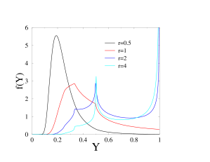
Figure 13: Distribution $f_{Y}(Y)$ of the quantity $Y$, for four characteristic values of the control parameter $r$.

The moments $\overline{Y^{k}}$ can be evaluated, at least in principle, by means of the identity

$$Y^{k}=\frac{S_{2}^{k}}{S_{1}^{2k}}=\frac{S_{2}^{k}}{(2k-1)!}\int_{0}^{\infty}\rme^{-tS_{1}}\,t^{2k-1}\,{\rm d}t.$$ (2.28)

The quantities $\overline{S_{2}^{k}\rme^{-tS_{1}}}$ can be calculated by expanding the result (2.22) as a Taylor series in $t_{2}$. Some algebra involving integrations by parts leads to the following integral expressions for the first two moments of $Y$:

$$\;\overline{Y}=1 - \frac{1}{r}\int_{0}^{\infty}\rme^{-F_{1}(t)/r}\,\rme^{-t}\,{\rm d}t,$$

$$\overline{Y^{2}}=1 - \frac{1}{6r}\int_{0}^{\infty}\rme^{-F_{1}(t)/r}\,\rme^{-t}(t^{2}+3t+5){\rm d}t$$ (2.29)

$$- \frac{1}{6r^{2}}\int_{0}^{\infty}\rme^{-F_{1}(t)/r}\,\rme^{-t}(2-(t+2)\rme^{-t}){\rm d}t.$$

Figure 14 shows plots of $\overline{Y}$ (left) and of $\mathop{\rm var}\nolimits{Y}$ (right), obtained by evaluating the above integrals numerically, against $r/(r+1)$. The variance reaches its maximum $\mathop{\rm var}\nolimits{Y}\approx 0.05218$ for $r\approx 2.25$.

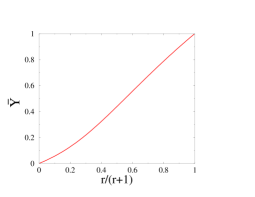
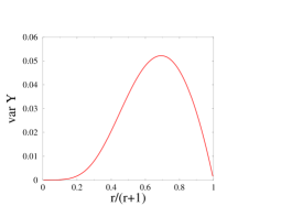
Figure 14: Plots of $\overline{Y}$ (left) and of $\mathop{\rm var}\nolimits{Y}$ (right), against $r/(r+1)$.

The mean value of the quantity $R=1/Y$ can be determined along the same line of thought. Some algebra using the identity

$$R=\frac{1}{Y}=\frac{S_{1}^{2}}{S_{2}}=S_{1}^{2}\int_{0}^{\infty}\rme^{-tS_{2}}\,{\rm d}t$$ (2.30)

leads to the following integral expression

$$\overline{R}=1+\frac{\pi}{4r^{2}}\int_{0}^{\infty}\rme^{-F_{1}(t)/(2r)}(\mathop{\rm erf}\nolimits\sqrt{t})^{2}\,\frac{{\rm d}t}{t}.$$ (2.31)

In the $r\ll 1$ regime, where the number of significant weights gets large, we obtain

$$\;\;\overline{Y} = \frac{r}{2}+\frac{r^{2}}{12}-\frac{r^{3}}{24}-\frac{101r^{4}}{720}+\cdots,$$

$$\mathop{\rm var}\nolimits{Y} = \frac{r^{3}}{2}+\frac{37r^{4}}{360}+\frac{7r^{5}}{90}+\cdots,$$

$$\;\;\overline{R} = \frac{2}{r}+\frac{1}{3}+\frac{14r}{15}+\cdots,$$ (2.32)

and so the distribution of $Y$ is asymptotically a narrow Gaussian around $r/2$, whose width scales as $r^{3/2}$.

In the opposite $r\gg 1$ regime, the distribution of $Y$ is dominated by a strong divergence as $Y\to 1$, and so the moments approach unity as

$$\;\;\overline{Y} = 1-\frac{1}{r}+\frac{\ln 2}{r^{2}}+\cdots,$$

$$\mathop{\rm var}\nolimits{Y} = \frac{1}{3r}-\frac{4\ln 2+7}{12r^{2}}+\cdots,$$

$$\;\;\overline{R} = 1+\frac{\pi}{2r}+\frac{\pi\ln 2-2{\bf C}}{2r^{2}}+\cdots,$$ (2.33)

where ${\bf C}=0.915\,965\dots$ denotes Catalan’s constant. This regime is studied in more detail in the next section.

B.4 Effective two-site model in the $r\gg 1$ regime

In the $r\gg 1$ regime, the (ordered) weights $\Pi_{m}=\rme^{-rx_{m}}$ fall off very rapidly with $m$. We are therefore led to consider an effective two-site model, where only the largest two weights are kept, while all the other ones are neglected. The corresponding Poissonian points are $x_{1}=\tau_{1}$ and $x_{2}=\tau_{1}+\tau_{2}$.

Within this framework, we have

$$S_{1}=\Pi_{1}+\Pi_{2}=\rme^{-r\tau_{1}}(1+\rme^{-r\tau_{2}}),$$

$$S_{2}=\Pi_{1}^{2}+\Pi_{2}^{2}=\rme^{-2r\tau_{1}}(1+\rme^{-2r\tau_{2}}),$$ (2.34)

and hence

$$Y=\frac{1+\rme^{-2r\tau_{2}}}{(1+\rme^{-r\tau_{2}})^{2}}.$$ (2.35)

The quantity $Y$ therefore only depends on $\tau_{2}$. It lives in the interval $1/2<Y<1$, and its distribution reads

$$f_{Y}(Y)=\frac{1}{r(1-Y)\sqrt{2Y-1}}\left(\frac{1-Y}{Y+\sqrt{2Y-1}}\right)^{1/r}.$$ (2.36)

This distribution exhibits an inverse-square-root singularity at the lower edge:

$$f_{Y}(Y)\approx\frac{2}{r\sqrt{2Y-1}}\qquad(Y\to 1/2),$$ (2.37)

and a very strong divergence at the upper edge:

$$f_{Y}(Y)\approx\frac{1}{r}(1-Y)^{-1+1/r}\qquad(Y\to 1).$$ (2.38)

As a consequence, all the moments of $Y$ approach unity according to

$$\overline{Y^{k}}=1-\frac{\mu_{k}}{r},$$ (2.39)

where the amplitude of the negative $1/r$ correction term reads

$$\mu_{k}=\int_{1/2}^{1}\frac{{\rm d}Y}{\sqrt{2Y-1}}\,\frac{1-Y^{k}}{1-Y}.$$ (2.40)

The generating series of these numbers can be evaluated as

$$M(z)=\sum_{k\geq 1}\mu_{k}z^{k} = \frac{z}{1-z}\int_{1/2}^{1}\frac{{\rm d}Y}{\sqrt{2Y-1}(1-zY)}$$ (2.41)

$$= \frac{1}{1-z}\sqrt{\frac{z}{2-z}}\ln\frac{1+\sqrt{z(2-z)}}{1-z}.$$

This expression yields the values $\mu_{1}=1$ and $\mu_{2}=5/3$ (in agreement with (2.33) to order $1/r$), $\mu_{3}=32/15$, $\mu_{4}=52/21$, $\mu_{5}=863/315$, and so on, as well as the linear recursion formula

$$(2k-1)\mu_{k}-(3k-2)\mu_{k-1}+(k-1)\mu_{k-2}=1,$$ (2.42)

and the asymptotic growth law $\mu_{k}\approx\ln(2k)+\gamma$.

Finally, the formal expression obtained by setting $k=-1$ in (2.40), i.e.,

$$\mu_{-1}=-\int_{1/2}^{1}\frac{{\rm d}Y}{Y\sqrt{2Y-1}}=-\frac{\pi}{2},$$ (2.43)

agrees with the expansion (2.33) for $\overline{R}$.

Appendix C Effective two-site model in the localized regime ($c>1$)

The effective model studied in B can be extended to the localized regime ($c>1$), in order to describe the rare events where the first two weights $\Pi_{1}$ and $\Pi_{2}$ are comparable. We still have $S_{1}=\Pi_{1}+\Pi_{2}$ and $S_{2}=\Pi_{1}^{2}+\Pi_{2}^{2}$, and so

$$Y=\frac{1+\eta^{2}}{(1+\eta)^{2}},\qquad R=\frac{(1+\eta)^{2}}{1+\eta^{2}}=1+\frac{2\eta}{1+\eta^{2}},$$ (3.1)

where the weight ratio $\eta=\Pi_{2}/\Pi_{1}$ reads (see (4.16))

$$\eta\approx\exp\left(-\frac{\Delta}{M^{1/c}}\left(x_{2}^{1/c}-x_{1}^{1/c}\right)\right).$$ (3.2)

Let us first evaluate the mean value of this ratio:

$$\overline{\eta}\approx\int_{0}^{\infty}\rme^{-x_{2}}{\rm d}x_{2}\int_{0}^{x_{2}}\exp\left(-\frac{\Delta}{M^{1/c}}\left(x_{2}^{1/c}-x_{1}^{1/c}\right)\right){\rm d}x_{1}.$$ (3.3)

The integral over $x_{1}$ is dominated by small values of the difference $\tau_{2}=x_{2}-x_{1}\sim M^{1/c}/\Delta\sim M^{-(1-1/c)}\ll 1$. Linearizing the argument of the exponential with respect to $\tau_{2}$, and integrating over $\tau_{2}$ first, we readily obtain

$$\overline{\eta}\approx c\,\Gamma(2-1/c)\,\frac{M^{1/c}}{\Delta}=\frac{c\,\Gamma(2-1/c)}{\rho-\rho_{c}}\,M^{-(1-1/c)}.$$ (3.4)

Higher moments of $\eta$ can be estimated by replacing in the above result $\Delta$ by the product $k\Delta$. We thus get immediately

$$\overline{\eta^{k}}\approx\frac{\overline{\eta}}{k}.$$ (3.5)

This result leads to the picture that $\eta$ is zero with very high probability, and of order unity with a small probability of order $\overline{\eta}$. The quantity $\overline{\eta}$ thus provides an operational estimate for the probability that $\Pi_{1}$ and $\Pi_{2}$ are comparable. This probability was already anticipated in section 4 to fall off as $M^{-(1-1/c)}$.

Finally, by expanding the expression (3.1) for $R$ as a power series in $\eta$, using (3.5), as well as the result

$$1-\frac{1}{3}+\frac{1}{5}-\frac{1}{7}+\cdots=\frac{\pi}{4},$$ (3.6)

we are left with the following quantitative estimate for the mean value of $R$ in the localized regime:

$$\overline{R}-1\approx\frac{\pi c\,\Gamma(2-1/c)}{2}\,\frac{M^{1/c}}{\Delta}=\frac{\pi c\,\Gamma(2-1/c)}{2(\rho-\rho_{c})}\,M^{-(1-1/c)}.$$ (3.7)

References

References

- [1] Spitzer F, 1970 Advances in Math. 5 246
- [2] Andjel E D, 1982 Ann. Prob. 10 525
- [3] Landim C and Kipnis C, 1999 Scaling Limits of Interacting Particle Systems (Berlin: Springer)
- [4] Evans M R, 2000 Braz. J. Phys. 30 42
- [5] Evans M R and Hanney T, 2005 J. Phys. A 38 R195
- [6] Godrèche C, 2007 Lect. Notes Phys. 716 261
- [7] Bialas P, Burda Z, and Johnston D, 1997 Nucl. Phys. B 493 505 Bialas P, Burda Z, and Johnston D, 1999 Nucl. Phys. B 542 413 Bialas P, Bogacz L, Burda Z, and Johnston D, 2000 Nucl. Phys. B 575 599
- [8] Drouffe J M, Godrèche C, and Camia F, 1998 J. Phys. A 31 L19
- [9] Godrèche C and Luck J M, 2001 Eur. Phys. J. B 23 473
- [10] Godrèche C, 2003 J. Phys. A 36 6313
- [11] O’Loan O J, Evans M R, and Cates M E, 1998 Phys. Rev. E 58 1404
- [12] Jeon I, March P, and Pittel B, 2000 Ann. Prob. 28 1162
- [13] Grosskinsky S, Schütz G M, and Spohn H, 2003 J. Stat. Phys. 113 389
- [14] Godrèche C and Luck J M, 2005 J. Phys. A 38 7215
- [15] Majumdar S N, Evans M R, and Zia R K P, 2005 Phys. Rev. Lett. 94 180601 Evans M R, Majumdar S N, and Zia R K P, 2006 J. Stat. Phys. 123 357
- [16] Evans M R and Majumdar S N, 2008 J. Stat. Mech. P05004
- [17] Armendariz I and Loulakis M, 2009 Probab. Th. Rel. Fields 145 175
- [18] Ferrari P A, Landim C, and Sisko V V, 2007 J. Stat. Phys. 128 1153
- [19] Beltrán J and Landim C, 2012 Probab. Th. Rel. Fields 152 781 Landim C, 2012 preprint arXiv:1204.5987
- [20] Benjamini I, Ferrari P A, and Landim C, 1996 Stochastic Process. Appl. 61 181
- [21] Krug J and Ferrari P A, 1996 J. Phys. A 29 L465
- [22] Evans M R, 1996 Europhys. Lett. 36 13
- [23] Andjel E D, Ferrari P A, Guiol H, and Landim C, 2000 Stochastic Process. Appl. 90 67
- [24] Jain K and Barma M, 2003 Phys. Rev. Lett. 91 135701
- [25] Angel A G, Evans M R, and Mukamel D, 2004 J. Stat. Mech. P04001
- [26] Landim C, 1996 Ann. Prob. 24 599
- [27] Noh J D, Shim G M, and Lee H, 2005 Phys. Rev. Lett. 94 198701 Noh J D, 2005 Phys. Rev. E 72 056123
- [28] Bogacz L, Burda Z, Janke W, and Waclaw B, 2007 Chaos 17 026112 Waclaw B, Bogacz L, Burda Z, and Janke W, 2007 Phys. Rev. E 76 046114 Waclaw B, Burda Z, and Janke W, 2008 Eur. Phys. J. B 65 565
- [29] Tang M, Liu Z, and Zhou J, 2006 Phys. Rev. E 74 036101 Tang M, Liu Z, Zhu X, and Wu X, 2008 Int. J. Mod. Phys. C 19 927
- [30] Ohkubo J, 2007 Phys. Rev. E 76 051108
- [31] Grosskinsky S, Chleboun P, and Schütz G, 2008 Phys. Rev. E 78 030101(R) del Molino L C G, Chleboun P, and Grosskinsky S, 2012 J. Phys. A 45 205001
- [32] Juhász R, Santen L, and Iglói F, 2005 Phys. Rev. Lett. 94 010601 Juhász R, Santen L, and Iglói F, 2005 Phys. Rev. E 72 046129 Juhász R, Santen L, and Iglói F, 2006 Phys. Rev. E 74 061101
- [33] Barma M, 2006 Physica A 372 22
- [34] van Leeuwen J M J and Kooiman A, 1992 Physica A 184 79
- [35] Alexander S, Bernasconi J, Schneider W R, and Orbach R, 1981 Rev. Mod. Phys. 53 175 Haus J W and Kehr K W, 1987 Phys. Rep. 150 263 Bouchaud J P and Georges A, 1990 Phys. Rep. 195 127 Ben-Avraham D and Havlin S, 2000 Diffusion and Reactions in Fractals and Disordered Systems (Cambridge: Cambridge University Press)
- [36] Coles S, 2001 An Introduction to Statistical Modeling of Extreme Values Springer Series in Statistics (London: Springer)
- [37] Derrida B and Flyvbjerg H, 1987 J. Phys. A 20 5273
- [38] Mirlin A D, 2000 Phys. Rep. 326 259
- [39] Albert R and Barabási A L, 2002 Rev. Mod. Phys. 74 47 Dorogovtsev S N and Mendes J F F, 2003 Evolution of Networks (Oxford: Oxford University Press) Barrat A, Barthélemy M, and Vespignani A, 2008 Dynamical Processes on Complex Networks (Cambridge: Cambridge University Press) Newman M E J, 2010 Networks: An Introduction (Oxford: Oxford University Press)
- [40] Krapivsky P L and Redner S, 2002 Phys. Rev. Lett. 89 258703
- [41] Godrèche C, Grandclaude H, and Luck J M, 2010 J. Stat. Mech. P02001
- [42] Schwarzkopf Y, Evans M R, and Mukamel D, 2008 J. Phys. A 41 205001
- [43] Thompson A G, Tailleur J, Cates M E, and Blythe R A, 2010 J. Stat. Mech. P02013
- [44] Evans M R, Hanney T, and Majumdar S N, 2006 Phys. Rev. Lett. 97 010602
- [45] Waclaw B, Sopik J, Janke W, and Meyer-Ortmanns H, 2009 Phys. Rev. Lett. 103 080602 Waclaw B, Sopik J, Janke W, and Meyer-Ortmanns H, 2009 J. Stat. Mech. P10021
- [46] Waclaw B and Evans M R, 2012 Phys. Rev. Lett. 108 070601
- [47] Luck J M and Godrèche C, 2007 J. Stat. Mech. P08005
- [48] Grosskinsky S, Redig F, and Vafayi K, 2011 J. Stat. Phys. 142 952
- [49] Hirschberg O, Mukamel D, and Schütz G M, 2009 Phys. Rev. Lett. 103 090602 Hirschberg O, Mukamel D, and Schütz G M, 2012 J. Stat. Mech. P08014
- [50] Kesten H, 1973 Acta Math. 131 208 Kesten H, Kozlov M V, and Spitzer F, 1975 Compos. Math. 30 145
- [51] Vervaat W, 1979 Adv. Appl. Prob. 11 750
- [52] Derrida B and Hilhorst H J, 1983 J. Phys. A 16 2641
- [53] de Calan C, Luck J M, Nieuwenhuizen T M, and Petritis D, 1985 J. Phys. A 18 501
- [54] Nieuwenhuizen T M and van Rossum M C W, 1991 Phys. Lett. A 160 461
- [55] Rényi A, 1958 Publ. Math. Inst. Hung. Acad. Sci. 3 109