Peaks in the CMBR power spectrum. I. Mathematical analysis of the associated real space features

Abstract

The purpose of our study is to understand the mathematical origin in real space of modulated and damped sinusoidal peaks observed in cosmic microwave background radiation anisotropies. We use the theory of the Fourier transform to connect localized features of the two-point correlation function in real space to oscillations in the power spectrum. We also illustrate analytically and by means of Monte Carlo simulations the angular correlation function for distributions of filled disks with fixed or variable radii capable of generating oscillations in the power spectrum. While the power spectrum shows repeated information in the form of multiple peaks and oscillations, the angular correlation function offers a more compact presentation that condenses all the information of the multiple peaks into a localized real space feature. We have seen that oscillations in the power spectrum arise when there is a discontinuity in a given derivative of the angular correlation function at a given angular distance. These kinds of discontinuities do not need to be abrupt in an infinitesimal range of angular distances but may also be smooth, and can be generated by simply distributing excesses of antenna temperature in filled disks of fixed or variable radii on the sky, provided that there is a non-null minimum radius and/or the maximum radius is constrained.

1 Introduction

We present a series of two papers with the motivation of understanding the CMBR (”Cosmic Microwave Background Radiation”) anisotropies[1] without direct comparison with a physical model, in order to see whether other conditions different from the standard model of cosmology may generate something similar of what is observed. In this first part, we will focus qualitatively on the mathematical elements necessary to produce peaks in the power spectrum of the CMBR, and in the second part [2] we will discuss its physical generic interpretation and evaluate quantitatively the number of free parameters a generic theory needs in order to fit it. This line of research is at present almost totally abandoned, the available literature merely discussing how the peaks can be generated in terms of the standard cosmology. We could consider our theme as an inversion problem: rather than deriving the predictions from a model to fit the data, we wish to ascertain from the data some general characteristics of a generic model. Our goal is to open analysis to wider mathematico–physical scenarios, in order to see whether something different from standard cosmology interpretation can reproduce it.

The analysis of CMB maps is usually performed in terms of spherical harmonic decomposition and by computing the angular power spectrum of CMB anisotropies [3, 4, 5, 6]. The standard cosmological model provides a physical model able to fit accurately the power spectrum of CMB anisotropies. It is well known that this exhibits a series of peaks, or an almost periodic oscillation, as predicted by Peebles & Yu [7].

In the ideal case of full-sky coverage, the two-point angular correlation function provides a complementary means of analyzing CMB observations instead of the angular power spectrum and, in principle, contains the same information as the angular power spectrum. However, as we will discuss in what follows, the angular correlation function allows an easier understanding of the anisotropy structures and it may serve as a complementary means of spherical harmonic analysis. Few authors have considered the direct determination of the anisotropies correlation function directly in angular space [8, 9, 10, 11, 12, 13, 14], (see the review in ref. [15]), and many of them have focused on the large scale behavior of the angular correlation function, where the effect of cosmic variance is certainly important. In particular, the two-point correlation function almost vanishes on scales greater than about 60 degrees, contrary to what the standard CDM theory predicts, and is in agreement with the same finding obtained from COBE data about a decade earlier[8, 9]. It was pointed out[15] that the striking feature of the two-point angular correlation function is the lack of large angle correlations, unexpected in inflationary models. On the other hand it is also interesting to consider, both theoretically and observationally, the behavior of the correlation function on small angular scales [16, 17]. Indeed, the whole structure of the peaks in the angular power spectrum corresponds in direct angular space to a localized feature of the correlation function which is analogous for the CMB field to the baryon acoustic oscillation (BAO) scale characterizing the matter correlation function [18, 19] (see criticism on its detection in ref. [20]). The direct identification of such a scale would thus represent a complementary test of the standard model.

In this paper, we illustrate some simple mathematical properties of the anisotropy structures associated with both the oscillating peaks in the angular power spectrum and with the characteristic scale in the anisotropy angular distribution. In particular, we provide a simple explanation of the peak sequence, showing that it is simply associated with the shape of the structures of the anisotropies. While this discussion is useful to illustrate the statistical meaning of the properties of the $\Lambda$-CDM angular correlation function, it also provides a simple general model to generate such type of correlations.

Our paper is structured as follows: In §2, we discuss the mathematical origin of the oscillating peaks in the power spectrum, and of the corresponding scales in the angular distribution of anisotropies. In §3, we illustrate the situation by introducing a few simple toy models able to show similar correlation properties as those predicted by standard cosmological models. Finally, in §4 we summarize the results.

2 The origin of oscillations in the power spectrum and its correspondence in the correlation function at small angles

2.1 Power spectrum and self-correlation

The fluctuation field on the sky, $\frac{\delta T}{T}(\hat{\bf n})$, where $\hat{\bf n}$ is the general point on the unit sphere (or direction in $3-$dim space), can be decomposed into spherical harmonics in the sphere:

$$\frac{\delta T}{T}(\hat{\bf n})=\sum_{\ell=0}^{\infty}\sum_{m=-\ell}^{+\ell}a_{\ell m}Y_{\ell m}(\hat{\bf n})\;.$$ (1)

Assuming statistical isotropy, the angular power spectrum $C_{\ell}$ is defined as

$$C_{\ell}\equiv\langle|a_{\ell m}|^{2}\rangle=\frac{1}{2\ell+1}\sum_{m=-\ell}^{+\ell}|a_{\ell m}|^{2}\;,$$ (2)

whereas the angular two-point correlation function is defined as [[21],[22](§6.6.1)]:

$$C(\theta)\equiv\left\langle\frac{\delta T}{T}(\hat{\bf n})\frac{\delta T}{T}(\hat{\bf n}^{\prime})\right\rangle$$ (3)

where $\theta$ is the separation angle between the two directions $\hat{\bf n}$ and $\hat{\bf n}^{\prime}$. The two-point correlation function can be expanded in terms of Legendre polynomials ($P_{\ell}$):

$$C(\theta)=\frac{1}{4\pi}\sum_{\ell=0}^{\infty}(2\ell+1)C_{\ell}P_{\ell}[\cos(\theta)]\;.$$ (4)

By inverting Eq. (4) we find[15]

$$C_{\ell}=2\pi\int_{0}^{\pi}C(\theta)P_{\ell}[\cos(\theta)]\sin(\theta)d\theta.$$ (5)

Alternatively, always assuming statistical isotropy, we can express the power spectrum in terms of the conjugate frequency $k$ in the Fourier transform:

$$P(k)=\tilde{C}(k)\equiv FT[C(\theta)]=\int d\vec{\theta}C(\theta)e^{-i\vec{k}\vec{\theta}},$$ (6)

where the vectors $\vec{\theta}$ and $\vec{k}$ are two-dimensional vectors whose moduli are $\theta$ and $k$ respectively, and

$$C(\theta)=FT^{-1}[P(k)]\;.$$ (7)

For small enough angles $\theta\ll 1$ radians, $P_{\ell}[\cos(\theta)]\approx J_{0}[(\ell+1/2)\theta]$ [23](Eq. 46.39), where $J_{0}$ is the Bessel function of order zero, and $P(k)\approx 2\pi\int_{0}^{\pi}C(\theta)$ $J_{0}(k\theta)\sin\theta d\theta$ [23](Eq. 46.43), so the spherical harmonic decomposition coincides with the two-dimensional Fourier transform with a frequency $k=(\ell+1/2)$. From now on, we will not distinguish between $C_{\ell}$ and $P(k)$.

2.2 Relationship between oscillations in the power spectrum and abrupt transitions in the self-correlation function

In order to clarify the relation between the sequence of oscillating peaks in the CMB angular power spectrum and the angular space two-point correlation function, let us introduce a simple model. We first distribute points centers uniformly in space and then distribute continuous mass profiles around these points, which hereafter we denominate as centers. Since we are interested in the angular correlation function $C(\theta)$ at $\theta\ll 1$ radians, we can approximate the angular space as Euclidean and use Fourier transform analysis to illustrate mathematically the link between sinusoidal oscillations in the power spectrum and strongly localized features in the two-point correlation function.

In general in a $d-$dimensional Euclidean space the model can be formulated as follows. Let us start with a stochastic spatial distribution of centers with microscopic number density

$$n({\bf x})=\sum_{i}\delta({\bf x}-{\bf x}_{i})\,,$$ (8)

where the sum runs over all center positions ${\bf x}_{i}$. Let us assume that this distribution is statistically homogeneous in space, which implies: (i) the average number density is a positive constant $n_{0}>0$, and (ii) the two-point correlation function (TPCF) depends only on the separation vector between these two points. In this case, the TPCF can be defined as [22]

$$\xi({\bf x})=\frac{\left<n({\bf x}_{0})n({\bf x}_{0}+{\bf x})\right>-n_{0}^{2}}{n_{0}^{2}}=\frac{\delta({\bf x})}{n_{0}}+h({\bf x})\,,$$ (9)

where $\left<\cdot\right>$ represents the ensemble average, or the infinite volume average in the case of ergodicity. We assume that $h({\bf x})$ (the covariance or off-diagonal correlation function) is a sufficiently regular function with no discontinuity in any of its derivatives for $x>0$ and decays sufficiently rapidly at large separations ${\bf x}$ (e.g., one can suppose an analytic function in all space ${\bf x}$ as an exponential or power law decay).

Due to the assumed statistical and spatial homogeneity, the power spectrum $S({\bf k})$ of the stochastic distribution of centers satisfies

$$S({\bf k})\equiv\lim_{V\to\infty}\frac{\left<|\delta\tilde{n}({\bf k};V)|^{2}\right>}{n_{0}V}=1+n_{0}\tilde{h}({\bf k})\,,$$ (10)

where

$$\delta\tilde{n}({\bf k};V)=\int_{V}d^{d}x[n({\bf x})-n_{0}]e^{-i{\bf k}\cdot{\bf x}}$$ (11)

$$\tilde{h}({\bf k})=FT[h({\bf x})]=\int_{\mathbb{R}^{d}}d^{d}x\,h({\bf x})e^{-i{\bf k}\cdot{\bf x}}\,.$$ (12)

Note that, since $\tilde{h}({\bf k})$ vanishes at large $k$, $S({\bf k})$ in the same limit converge to $1$. As shown more rigorously below, since $h({\bf x})$ is thought to have all continuous derivatives at $x>0$, $S({\bf k})$ is expected not to present damped sinusoidal oscillations.

Let us now replace each center at ${\bf x}_{i}$ with a continuous density profile described by the function $f({\bf x}-{\bf x}_{i})\geq 0$, such that $f({\bf x}\to\infty)\to 0$ sufficiently fast so that $\int_{\mathbb{R}^{d}}d^{d}x\,f({\bf x})$ is equal to a finite positive constant which we can take to be $1$. The field can now be written as

$$T({\bf x})=\sum_{i}f({\bf x}-{\bf x}_{i})\,.$$ (13)

The mean value is clearly $\left<T({\bf x})\right>=n_{0}\int d^{d}x\,f({\bf x})$.

Since we can write

$$T({\bf x})=\int d^{d}yf({\bf x}-{\bf y})n({\bf y})\,,$$ (14)

it is simple to show that the power spectrum $P({\bf k})$ of the field $T({\bf x})$ is simply given by

$$P({\bf k})=|\tilde{f}({\bf k})|^{2}S({\bf k})\,,$$ (15)

where $\tilde{f}({\bf k})=FT[f({\bf x})]$. Note that, as $f({\bf x})$ is assumed to be integrable, $\tilde{f}({\bf k})$ vanishes at large $k$ and therefore also $P({\bf k})$ vanishes at large $k$. At the same time, the TPCF of the field $T({\bf x})$ is a continuous function, as it has to be for any proper continuous field[22].

Since we have assumed that $S({\bf k})$ is not characterized by oscillating peaks, if we want $P({\bf k})$ to show them, we need these to be associated with $\tilde{f}({\bf k})$. Thus, the problem is reduced to finding which features of $f({\bf x})$ generate oscillating peaks in $P({\bf k})$. We show below that if $f({\bf x})$ presents a finite discontinuity in the function or in one of its derivatives at a position ${\bf x}_{0}\neq 0$, then $P({\bf k})$ will show slowly damped sinusoidal oscillations and wave-vector peaks (in Fourier space) ${\bf x}_{0}$.

A simple example is given by the following function $f({\bf x})$ in $d$ dimensions, usually called spherical box function

$$f({\bf x})=\left\{\begin{array}[]{ll}1/\|S_{d}(R)\|&\mbox{for }{\bf x}\in S_{d}(R)\\ 0&\mbox{otherwise}\end{array}\right.$$

where $S_{d}(R)$ is the $d-$dimensional sphere of radius $R$ centered at the origin and $\|S_{d}(R)\|$ its volume. In this case, $\tilde{f}({\bf k})$ is characterized by slowly damped sinusoidal oscillations:

$$\tilde{f}(k)=\left\{\begin{array}[]{ll}\frac{\sin(kR)}{kR},&\mbox{$d=1$}\\ \frac{2}{kR}J_{1}(kR),&\mbox{$d=2$}\\ 3\frac{\sin(kR)-kR\cos(kR)}{(kR)^{3}},&\mbox{$d=3$}\end{array}\right\}\;,$$ (16)

where $J_{1}$ is the Bessel function of the first kind. If, for example, we have a Poissonian distribution of centers, i.e., one with $S({\bf k})=1$, we have simply $P({\bf k})=|\tilde{f}(k)|^{2}$ which shows slowly damped sinusoidally oscillating peaks. A generalization of this development for a variable radius $R$ is given in the following subsection.

2.3 Mathematical description of the origin of oscillations in the varying radius case

We can generalize the mathematical description of §2.2 for variable radius balls by considering the following field

$$T({\bf x})=\sum_{i}f({\bf x}-{\bf x}_{i};R_{i})\,,$$ (17)

where $\{{\bf x}_{i}\}$ are the positions of the centers and

$$f({\bf x};R_{i})=A(R_{i})g(x)\theta(R_{i}-x)\,,$$

where the radius $R_{i}$ changes from center to center, $g(x)$ is an arbitrary universal non-negative function and $A(R_{i})$ is the probability density function.

In order to find the power spectrum $P({\bf k})$ we should calculate the following double average

$$P({\bf k})=\frac{\left<\overline{|\delta\tilde{T}({\bf k},V)|^{2}}\right>}{T_{0}V}\,,$$

where $\delta\tilde{T}({\bf k},V)=FT_{V}[T({\bf x})-T_{0}]$, $\left<\cdot\right>$ is the ensemble average over the positions of centers and $\overline{(\cdot)}$ is the average over the distributions of radii. The two averages clearly commute. The first step is to write

$$\tilde{T}({\bf k},V)=\int_{V}d^{d}xT({\bf x})e^{-i{\bf k}\cdot{\bf x}}=\sum_{i}e^{-i{\bf k}\cdot{\bf x}_{i}}\tilde{f}({\bf k};R_{i})\,.$$

We can then write

$$|\tilde{T}({\bf k},V)|^{2}=\sum_{i,j}\tilde{f}({\bf k},R_{i})\tilde{f}({\bf k},R_{j})e^{-i{\bf k}\cdot({\bf x}_{i}-{\bf x}_{j})}\,.$$

It is simple to show that the diagonal part of this double sum is exactly balanced by the subtraction of the mean density from $T({\bf x})$ in the actual definition of the PS, for this reason only the non-diagonal part contributes to the final PS. We have therefore to calculate the following average

$$\overline{|\tilde{T}({\bf k},V)|^{2}}=\left[\overline{\tilde{f}({\bf k};R)}\right]^{2}\sum_{i,j}^{\prime}e^{-i{\bf k}\cdot({\bf x}_{i}-{\bf x}_{j})}\,,$$ (18)

where the prime in the double sum means the condition $i\neq j$, and

$$\overline{\tilde{f}({\bf k};R)}=\int d^{d}x\,e^{-i{\bf k}\cdot{\bf x}}g(x)\int_{-\infty}^{+\infty}dR\,A(R)\theta(R-x)\,.$$

By taking the second average $\left<\cdot\right>$ of Eq. (18), finally we get

$$P({\bf k})=\left[\overline{\tilde{f}({\bf k};R)}\right]^{2}S({\bf k})\,.$$

Thus the problem is reduced to calculating $\overline{\tilde{f}({\bf k};R)}$.

In other words, the power spectrum is the superposition of the power spectra for each value of $R_{i}$.

2.4 General relation between singular points in a function and damped oscillations in its FT

Let us now give the general argument relating the discontinuity of the function $f({\bf x})$, or of one of its derivatives at some point ${\bf x}_{0}\neq 0$ to the presence of slowly (i.e., power law) damped oscillations (and peaks) in $P({\bf k})$. With the aim of simplicity let us develop the argument in $d=1$ dimensions. Let us assume that the function $f(x)$ is analytic everywhere with the exception of the point $x_{0}$ where its $n^{th}$ derivative $f^{(n)}(x)$ presents a finite discontinuity: $f^{(n)}(x_{0}^{+})-f^{(n)}(x_{0}^{-})=A$. Moreover, let us assume that $f(x)$ vanishes sufficiently rapidly at large $|x|$. Let us study the features of the FT of $f(x)$ induced by such discontinuities. The FT is defined by

$$\tilde{f}(k)=\int_{-\infty}^{+\infty}dx\,e^{-ikx}f(x)\,.$$ (19)

By integrating it by parts $n+1$ times, we get

$$\tilde{f}(k)=\frac{1}{(ik)^{n+1}}\int_{-\infty}^{+\infty}dx\,e^{-ikx}f^{(n+1)}(x)$$ (20)

$$=\frac{1}{(ik)^{n+1}}\lim_{\epsilon,\epsilon^{\prime}\to 0}\left[\int_{-\infty}^{x_{0}-\epsilon}dx\,e^{-ikx}f^{(n+1)}(x)+\right.$$

$$\left.\int_{x_{0}+\epsilon^{\prime}}^{+\infty}dx\,e^{-ikx}f^{(n+1)}(x)+A\int_{x_{0}-\epsilon}^{x_{0}+\epsilon^{\prime}}dx\,e^{-ikx}\delta(x-x_{0})\right]$$

$$=\frac{1}{(ik)^{n+1}}\int_{-\infty}^{+\infty}dx\,e^{-ikx}g(x)+\frac{Ae^{-ikx_{0}}}{(ik)^{n+1}}\,,$$

where

$$g(x)=f^{(n+1)}(x)-A\delta(x-x_{0})$$

is an analytic function everywhere but in $x_{0}$ where at most it can have a finite discontinuity. In this last case this discontinuity will lead to a further, but subdominant (i.e., decreasing faster with $k$) contribution to the slowly damped oscillations given by the last term in Eq. (20). It is important to note that the power of decay of damped oscillations is directly related to the order of the discontinuous derivative.

This argument can be extended to higher dimensions. For a statistically isotropic distribution in $d$ dimensions in which both $f({\bf x})$ and $\xi({\bf x})$ depend only on $x=|{\bf x}|$, and consequently $\tilde{f}({\bf k})$, $S({\bf k})$ and $P({\bf k})$ depend only on $k=|{\bf k}|$. In this case, when $f({\bf x})\equiv f(x)$ shows a discontinuity in only one of the derivatives in $x$, the calculation can be reduced to a one-dimensional one very similar to the one-dimensional case treated above.

The terms $\exp(-ikx_{0})$ in Eq. (20) give the oscillations. Thus oscillating peaks in the power spectrum occur when the correlation function has an abrupt change of functionality at some $\theta_{0}>0$; that is, when there is a characteristic angular distance which separates two regimes in the self-correlation $C(\theta)$; mathematically, this means that some derivative is not continuous at this point. For our case, $d=2$, this happens in any TPCF such that

$$C(\theta)=\left\{\begin{array}[]{ll}g_{1}(\theta),&\mbox{$\theta\leq\theta_{0}$}\\ g_{2}(\theta),&\mbox{$\theta>\theta_{0}$}\end{array}\right\}\;,$$ (21)

with $g_{1}^{(n)}(\theta_{0}^{-})\neq g_{2}^{(n)}(\theta_{0}^{+})$.

The exact structure of the oscillations depends both on the point with some non-continuous derivative, $\theta_{0}$, and also on the slope before and after that point: $g_{1}(\theta_{0}^{-})$ and $g_{2}(\theta_{0}^{+})$. In general, it may also happen that there is more than one point with a point of this kind. In the case of CMBR analysis, one point with some non-continuous derivative is enough to explain all the peaks[2, 17, 11].

3 Examples and toy models

In order to make explicit the discussion in Sect. 2 let us consider the following two TPCF $C_{1}(\theta)$ and $C_{2}(\theta)$:

$$C_{1}(\theta)=A_{1,1}\exp(-\theta/\theta_{1,1})+A_{1,2}\exp(-\theta/\theta_{1,2})\,,$$

where we have chosen the following numerical values: $A_{1,1}=9744,A_{1,2}=3000,\theta_{1,1}=0.45,\theta_{1,2}=13.0$ (angles are in degrees), and

$$C_{2}(\theta)=\left\{\begin{array}[]{ll}A_{2,1}\exp(-\theta/\theta_{2,1}),&\mbox{$\theta\leq\theta_{*}$}\\ A_{2,2}\exp(-\theta/\theta_{2,2}),&\mbox{$\theta>\theta_{*}$}\end{array}\right.\;,$$

where $A_{2,1}=12000,A_{2,2}=3600,\theta_{2,1}=0.79,\theta_{1,2}=11.45,\theta_{*}=1.03$.

In Fig. 1, we plot these two correlation functions and their corresponding power spectra, derived through Eq. (5).

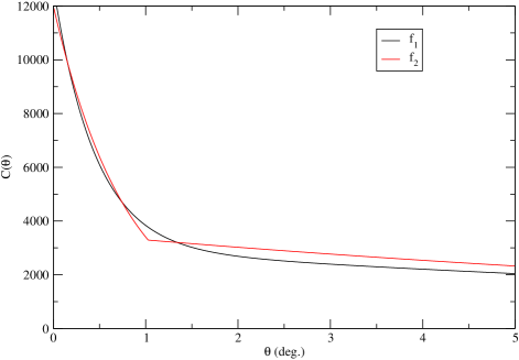
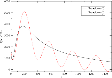
Figure 1: Upper panel: Test correlation functions $C_{1}(\theta)$ and $C_{2}(\theta)$. Bottom panel: The corresponding power spectra $FT[C_{1}]$ and $FT[C_{2}]$.

While both correlation functions present a relatively fast change in behavior at $\theta\approx 1^{\circ}$, only the power spectrum of $C_{2}(\theta)$ presents an oscillating series of peaks.

This simple example clearly shows that only the Fourier transform of a function which has a discontinuous derivative (i.e., $C_{2}(\theta)$) presents a series of oscillating peaks.

Let us now consider two illustrative toy models, constructed following the recipe discussed in Sect. 2.2.

3.1 Toy model 1: disks with same radius

We construct a statistically isotropic temperature field $T(\hat{\bf n})$ as follows. We distribute disks of angular radius $R$ such that for separation angles from the center of each disc $\theta\leq R$ the temperature field is $T(\hat{\bf n})=f(\theta_{r})$, $\theta_{r}$ being the distance from the center of the disk and the value of the field outside the disks being $T=0$. There are $N_{c}$ disks in a given angular region; their centers are distributed as a spatially homogeneous stochastic point process with an angular two-point correlation function $\omega(\theta)$. When $\omega(\theta)=0$ for $\theta>0$ the centers of the disks are distributed as a homogeneous spatial Poisson process. Given that we are interested in low values of $\theta\ll 1$ (radians), we can use the approximation $\sin(\theta)\approx\theta$.

Figure 2: Representation of the geometrical relationships between two points $i$, $j$ at two disks.

The self-correlation of the field $T$ corresponds to the integration over all possible pairs of points $(i,j)$ respectively within two disks (see Fig. 2). The self correlation is the average of the product of the value of the temperature in the first disk, $f(\theta_{i})$, multiplied by the value of the temperature in the second disk, $f(\theta_{j})$. The cases in which some point $i$ or $j$ is not within some disk give a null contribution to the integral. Therefore, our problem reduces to constraining the limits of the integral of the average correlation within the cases with non-null contribution. The problem is not trivial but, after a patient analysis, one can see that the solution is given by:

$$C(\theta)=\frac{N_{c}}{4\pi\ 2\pi\theta}\int_{0}^{2\pi}d\phi_{i}$$ (22)

$$\times\int_{0}^{R}d\theta_{i}\theta_{i}f(\theta_{i})[I_{s}(\theta,\theta_{i})+I_{o}(\theta,\theta_{i})],$$

where $I_{s}d\theta$ and $I_{o}d\theta$ stand for the integrals of the value of $T$ over all pixels $\vec{x}_{j}$ such that $\theta<|\vec{x}_{i}-\vec{x}_{j}|<\theta+d\theta$ respectively in the areas of the same circle of $\vec{x}_{i}$ ($I_{s}$) and in the areas of other disks ($I_{o}$). They do not depend on $\phi_{i}$ because both $f$ and $\omega$ depend only on the angular distance.

$I_{s}$ is an integral of the second areas in the case that $i$ and $j$ are in the same disk, integrating over all possible values of $\theta_{j}$, $\phi_{j}$ that keep the distance between the points $i$ and $j$ between $\theta$ and $\theta+d\theta$. It is:

$$I_{s}(\theta,\theta_{i})d\theta=\int_{0}^{2\pi}d\phi_{j}\int_{0;\theta<|\vec{x}_{i}-\vec{x}_{j}|<\theta+d\theta}^{R}d\theta_{j}\theta_{j}f(\theta_{j})$$ (23)

$$=\int_{0}^{2\pi}d\phi_{j}\theta_{j}(\theta,\theta_{i},\phi_{j})f[\theta_{j}(\theta,\theta_{i},\phi_{j})]\left|\frac{\partial\theta_{j}(\theta,\theta_{i},\phi_{j})}{\partial\theta}\right|d\theta.$$

The evaluation of $\theta_{j}$ is a function of $\theta$, $\theta_{i}$, $\phi_{j}$, such that $|\vec{x}_{i}-\vec{x}_{j}|=\theta$:

$$\theta_{j}(\theta,\theta_{i},\phi_{j})=\theta_{i}\cos(\phi_{j})\pm\sqrt{\Delta}$$ (24)

$$\Delta=\theta_{i}^{2}\cos(\phi_{j})^{2}-\theta_{i}^{2}+\theta^{2}$$

$$\mbox{where}\;\;\Delta\geq 0;0\leq\theta_{j}\leq R\;.$$

If, within the constraint, there are two possible values of $\theta_{j}$, both will contribute to the integral in Eq. (23), while if there are no values of $\theta_{j}$ no value will be included in the integral. This is a special case of Eq. (28) for $\theta_{o}=0$.

For the evaluation of the second integral involving $I_{o}$, we have to do something similar but moving the center of the disk $j$ among all possibilities. The center of the “other” disk is at angular distance $\theta_{o}$ from the first one, and azimuth $\phi_{o}$. Thus,

$$I_{o}(\theta,\theta_{i})d\theta=\int_{0}^{2\pi}d\phi_{o}\int_{0}^{\infty}d\theta_{o}\theta_{o}P(\theta_{o})$$ (25)

$$\times\int_{0}^{2\pi}d\phi_{j}\int_{0;\theta<|\vec{x}_{i}-\vec{x}_{j}|<\theta+d\theta}^{R}d\theta_{j}\theta_{j}f(\theta_{j})=$$

$$\int_{0}^{2\pi}d\phi_{o}\int_{0}^{\infty}d\theta_{o}\theta_{o}P(\theta_{o})$$

$$\times\int_{0}^{2\pi}d\phi_{j}\theta_{j}(\theta,\theta_{i},\phi_{j},\theta_{o},\phi_{o})f[\theta_{j}(\theta,\theta_{i},\phi_{j},\theta_{o},\phi_{o})]$$

$$\times\left|\frac{\partial\theta_{j}(\theta,\theta_{i},\phi_{j},\theta_{o},\phi_{o})}{\partial\theta}\right|d\theta$$

where $P(\theta_{o})$ is the probability per unit area of finding a circle at distance $\theta_{o}$ from the center of the first circle. $\theta_{j}$ is a function $\theta$, $\theta_{i}$, $\phi_{j}$, $\theta_{0}$, $\phi_{o}$ standing again for the value of $\theta_{j}$, which follows $|\vec{x}_{i}-\vec{x}_{j}|=\theta$ but taking into account that $\theta_{j}$ and $\phi_{j}$ are coordinates with respect to a second circle whose center is at coordinates $\theta_{o}$, $\phi_{o}$ with respect to the first one. In addition, by definition we have:

$$P(\theta_{o})=\frac{N_{c}}{4\pi}[1+\omega(\theta_{o})]\;.$$ (26)

For the calculation of $\theta_{j}$, by considering the two-dimensional planar approximation (instead of spherical geometry) illustrated in Fig. 2 we find

$$\theta=|\vec{x}_{i}-\vec{x}_{j}|\;,$$ (27)

$$\vec{x}_{i}=\theta_{i}\vec{i}\;,$$

$$\vec{x}_{j}=\theta_{o}(\cos\phi_{o}\vec{i}+\sin\phi_{o}\vec{j})+\theta_{j}(\cos\phi_{j}\vec{i}+\sin\phi_{j}\vec{j})\;.$$

Hence,

$$\theta_{j}(\theta,\theta_{i},\phi_{j},\theta_{o},\phi_{o})=-\theta_{o}\cos(\phi_{o}-\phi_{j})+\theta_{i}\cos(\phi_{j})$$ (28)

$$\pm\sqrt{\Delta}$$

$$\Delta=[\theta_{o}\cos(\phi_{o}-\phi_{j})-\theta_{i}\cos(\phi_{j})]^{2}-\theta_{o}^{2}-\theta_{i}^{2}+\theta^{2}$$

$$+2\theta_{i}\theta_{o}\cos(\phi_{o})$$

$$\mbox{where}\;\;\;\Delta\geq 0;0\leq\theta_{j}\leq R\;.$$

As in the previous case, if there are two possible values of $\theta_{j}$, both of them contributing to the integral in Eq. (25), while if there are no values of $\theta_{j}$ within the constraint, no value will be included in the integral.

The results of this toy model for some test functions are given in Fig. 3 respectively for:

a) $f(\theta)=1$ (homogeneous distribution within the disk), $\omega(\theta)=0$ (Poissonian distribution of disks), $R=1^{\circ}$, $N_{c}=10^{3}$;

b) $f(\theta)=1$, and

$$\omega(\theta)=\left\{\begin{array}[]{ll}-1,&\mbox{$\theta\leq 2R$}\\ 0,&\mbox{$\theta>2R$}\end{array}\right\}$$ (31)

i.e., a Poissonian distribution, with the added restriction that disks do not intersect, $R=1^{\circ}$, $N_{c}=10^{3}$;

c) $f(\theta)=1$, $\omega(\theta)=2\times\exp(-\theta/R)-1$, $R=1^{\circ}$, $N_{c}=10^{3}$;

d) $f(\theta)=\exp(-\theta/R)$, $\omega(\theta)=2\exp(-\theta/R)-1$, $R=1^{\circ}$, $N_{c}=10^{3}$.

We have also carried out Monte Carlo simulations: We have randomly distributed $N_{c}$ centers, with or without the constraint that minimal distance between two nearest neighboring centers is larger than $2R$, where $R$ is the disk’s size. Inside each disk of size $R$ we randomly distribute $N_{p}$ points. When disks are in a non-overlapping condition the minimal distance between the $N_{c}$ centers has to be $>2R$. We have chosen $R=1^{\circ}$ and we distribute $N_{c}=80$ disks in a square of side $L=1$ rad., in addition we fixed $N_{c}=1256$; the correlation functions are computed as an average over 50 realizations of the distribution. The results of the analytical calculation of cases 1a) and 1b) were compared with these Monte Carlo simulations (with the appropriate normalization to get the same value of $f(\theta<1^{\circ})=1$). The results are plotted in Fig. 3: numerical simulations nicely agree with analytical calculations.

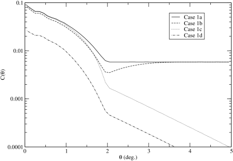
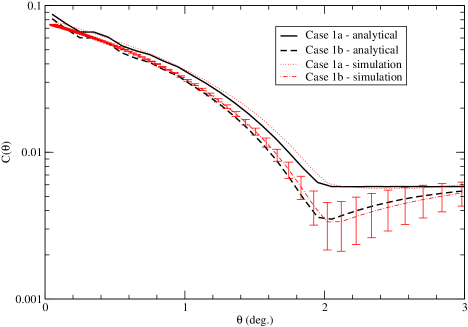
Figure 3: Upper panel: Self-correlation $C(\theta)$ for “toy-model 1” cases: a) $f(\theta)=1$, Poissonian distribution of disks; b) as in case $a$ but with the added restriction that disks do not intersect); c) as in case $a$ with two-point angular correlation function of the centers of disks $\omega(\theta)=2\times exp(-\theta/R)-1$; d) as in case $c$ but with $f(\theta)=exp(-\theta/R)$. All the cases with a number of disks $N_{c}=10^{3}$ of radius $R=1^{\circ}$. Bottom panel: Comparison of cases 1a) and 1b) derived analytically with the results of Monte Carlo simulations; with the error bars, we give the r.m.s. of the simulation 1b); for case 1a) is similar.

3.2 Toy model 2: disks with varying radii

With regard to disks of different size, we consider only the case in which $\omega(\theta)=0$, i.e., a Poisson distribution of disk centers. In the more general case of $\omega(\theta)\neq 0$, the shape of $C(\theta)$ would be changed, as we have seen in the previous subsection. However the feature corresponding to the abrupt transition [i.e., a discontinuous first derivative of $C(\theta)$], which is the scale of interest for the generation of the oscillating sequence of peaks in the angular power spectrum, does not depend on the particular shape of $\omega(\theta)$. We are going to show that the angular TPCF of the set of disks of different size is again characterized by a discontinuous derivative.

Let us assume that we have disks of different angular sizes $R$, and that, conditioned by their size, the contribution to the angular correlation function of disks with radius between $R$ and $R+dR$ follows a dependence

$$C(\theta,R)=\left\{\begin{array}[]{ll}A(R)h(\theta/R),&\mbox{$\theta\leq 2R$}\\ 0,&\mbox{$\theta>2R$}\end{array}\right.\;,$$ (32)

where $A(R)$ is the amplitude of the correlation of disks with radius $R$, and $h$ is a smooth continuous function with all continuous derivatives such that $h(2)=0$; such a distribution of $h$ is given by the contribution to the correlation of the disks with the same size (i.e., the toy model discussed in the previous section); we subtract the average field [thus, the constant $C(\theta>2R)$ may be set as zero conveniently defining a new $T^{*}=T-constant$]. Assuming a uniform distribution of radii between $R_{\rm min}$ and $R_{\rm max}$, given that there is no correlation between the positions of the disks, the angular TPCF is just the sum of the correlation function between its minimum and maximum radii. That is,

$$C(\theta)=\int_{R_{min}}^{R_{max}}C(\theta,R)dR=$$ (33)

$$\left\{\begin{array}[]{ll}\theta\int_{\theta/R_{max}}^{\theta/R_{min}}dxA(\theta/x)h(x)/x^{2},&\mbox{$\theta\leq 2R_{min}$}\\ \theta\int_{\theta/R_{max}}^{2}dxA(\theta/x)h(x)/x^{2},&\mbox{$2R_{min}<\theta<2R_{max}$}\\ 0,&\mbox{$\theta\geq 2R_{max}$}\end{array}\right.\;.$$ (37)

If there are minimum and maximum radii there is clearly a change of dependence with $\theta$ for three regimes. If, instead, there is only a minimum ($R_{min}>0$) or a maximum radius, there will be two regimes. Finally, if $R_{min}=0$, $R_{max}=\infty$, then there will be only one regime and no abrupt transition.

Let us consider an example: a) $A=1$, $h(x)=(1-x/2)$, for which we get

$$C(\theta)=$$ (38)

$$\left\{\begin{array}[]{ll}(R_{max}-R_{min})-\frac{1}{2}ln(R_{max}/R_{min})\theta,&\mbox{$\theta\leq 2R_{min}$}\\ R_{max}-\frac{1+ln(2)}{2}\theta+\frac{1}{2}ln(\theta/R_{max}),&\mbox{$2R_{min}<\theta<2R_{max}$}\\ 0,&\mbox{$\theta\geq 2R_{max}$}\end{array}\right.\;.$$

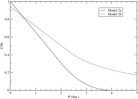
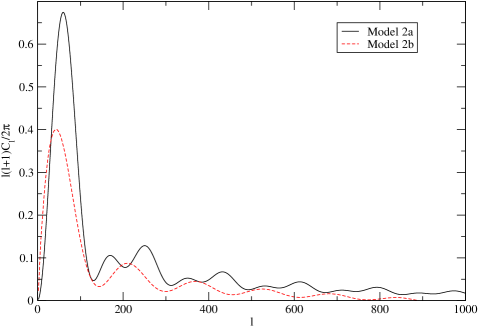
Figure 4: Upper panel: Two-point correlation $C(\theta)$ for the disks of varying radius, when no correlation among disk centers is considered a), b). Bottom panel: The corresponding power spectra.

Fig. 4 displays Eq. (38) for $R_{min}=1^{\circ}$ and $R_{max}=2^{\circ}$.

To each disk radius projected on the sky we could associate the physical distance $R=L/r$, where $r$ is the distance and $L$ is the physical size in an Euclidean space. As it will be discussed in [2], this may be representative of spheres placed at different distances. For $A(R)=\left(\frac{A_{0}}{R}\right)^{2}$ and for instance $h(x)=(1-x/2)$, we find

$$C(\theta)=$$ (39)

$$\left\{\begin{array}[]{ll}A_{0}^{2}[\frac{r_{max}-r_{min}}{L}-\frac{1}{4L^{2}}(r_{max}^{2}-r_{min}^{2})\theta],&\mbox{$\theta\leq\theta_{1}$}\\ A_{0}^{2}[-\frac{r_{min}}{L}+\frac{1}{\theta}+\frac{r_{min}^{2}}{4L^{2}}\theta],&\mbox{$\theta_{1}<\theta<\theta_{2}$}\\ 0,&\mbox{$\theta\geq\theta_{2}$}\end{array}\right.,$$

$$\theta_{1}\equiv 2L/r_{\rm max};\ \ \theta_{2}\equiv 2L/r_{\rm min}$$

Fig. 4 displays Eq. (39) for a case b) $A_{0}=0.02$, $r_{min}/L=3$, $r_{max}/L=50$.

As can be observed, the correlation function is smoother. However, the power spectra (Fig. 4) still show a sequence of oscillating peaks. Indeed, another way to understand the fact that oscillations are still present when the disk size is not fixed is obtained recalling that the power spectrum is the superposition of the power spectra for each radius (see §2.3): the superposition of oscillating power spectra gives still a global oscillation, provided they do not cancel each other out (which is the case when there is no minimum and/or maximum radius).

The examples of this subsection are some particular ways of convolution. In general, any kind of convolution or smoothing in the abruptness of the disc shape will also produce oscillations, though with damped amplitude of the oscillation.

4 Conclusions

Although the power spectrum analysis is useful for obtaining some kind of information on CMBR anisotropy data, the angular TPCF (Two-point correlation function) analysis gives a more straightforward physical representation of that distribution. Moreover, while the power spectrum shows repeated information in the form of its multiple peaks and oscillations, the TPCF, its Fourier transform, offers a compacter presentation which condenses all the information of the multiple peaks in a localized real space feature. Precisely because of that, and because there is a dearth of literature analyzing the properties of the TPCF, we have concentrated here on its analysis.

In this paper we have shown how oscillations in the power spectrum arise when there are some point singularities in the angular TPCF in the form of some discontinuity point of its $n$-th derivative at some angular distance. In particular, we have clarified the analytical link between the frequency and the power law order decay of damped oscillations in the power spectrum and the kind of singularity in the TPCF. We have then presented toy models able to generate and illustrate this phenomenology: simply by placing some distribution in the sky of filled disks of fixed or variable radii with an excess of antenna temperature, provided there is a minimum$>0$ and/or a maximum in the range of radii. Disks of different radii may stand for projection of spheres with variable radii or spheres with variable/fixed radii and variable distance from the observer.

Discussions on the physical interpretation of these mathematical properties for the case of CMB anisotropies and comparison with real CMBR data will be given in [2]. This paper, now in preparation, will discuss these mathematical properties in terms of matter distribution in the fluid which is generating the radiation. The angular correlation function of the anisotropies from CMBR data will also be calculated, in an effort to derive the minimum number of parameters of a generic function to fit it. The paper [2] will argue that a power spectrum with oscillations is a rather normal characteristic expected from any fluid with clouds of overdensities that emit/absorb radiation or interact gravitationally with the photons, and with a finite range of sizes and distances for those clouds. It will also show that the angular correlation function can be fitted by a generic function with a total of $\approx 6$ free parameters. The standard cosmological interpretation of “acoustic” peaks is just a particular case; peaks in the power spectrum might be generated in scenarios that have nothing to do with oscillations due to gravitational compression in a fluid. Nonetheless, the standard model with six free parameters produces a better fit than the generic fit with the same number of free parameters; it fits third and higher order peaks whereas the generic fit reproduces only the first two peaks.

Apart from the analysis of CMBR peaks, the concepts analyzed in this paper are general and applicable to any kind of power spectrum with oscillations/peaks. The BAO oscillations in the large-scale structure[19] might be, for instance, another field where these results can be applied.

References

- [1] M. White, D. Scott, J. Silk, Anisotropies in the Cosmic Microwave Background, Ann. Rev. Astron. Astrophys. 32 (1994) 319–370.
- [2] M. López-Corredoira, Peaks in the CMBR power spectrum. II. Physical interpretation for any cosmological scenario, in preparation (2012).
- [3] M. Tristram, G. Patanchon, J.F. Macías-Pérez, et al., The CMB temperature power spectrum from an improved analysis of the Archeops data, Astron. Astrophys. 436 (2005) 785–797.
- [4] H.V. Peiris, L. Verde, The shape of the primordial power spectrum: A last stand before Planck data, Phys. Rev. D 81(2) (2010) id. 021302.
- [5] D. Larson, J. Dunkley, G. Hinshaw, et al., Seven-year Wilkinson Microwave Anisotropy Probe (WMAP) Observations: Power Spectra and WMAP-derived Parameters, Astrophys. J. Supp. Ser. 192 (2011) id. 16.
- [6] S. Das, T.A. Marriage, P.A.R. Ade, et al., The Atacama Cosmology Telescope: A Measurement of the Cosmic Microwave Background Power Spectrum at 148 and 218 GHz from the 2008 Southern Survey, Astrophys. J. 729 (2011) id. 62.
- [7] P.J.E. Peebles, J.T. Yu, Primeval Adiabatic Perturbation in an Expanding Universe, Astrophys. J. 162 (1970) 815–836.
- [8] G.F. Smoot, C.L. Bennett, A. Kogut, et al., Structure in the COBE differential microwave radiometer first-year maps, Astrophys. J. 396 (1992) L1–L5.
- [9] G. Hinshaw, A.J. Banday, C.L. Bennett, et al., Two-Point Correlations in the COBE DMR Four-Year Anisotropy Maps, Astrophys. J. 464 (1996) L25–L28.
- [10] A. Kashlinsky, C. Hernández-Monteagudo, F. Atrio-Barandela, Determining Cosmic Microwave Background Structure from Its Peak Distribution, Astrophys. J. 557 (2001) L1–L5.
- [11] C. Hernández-Monteagudo, A. Kashlinsky, F. Atrio-Barandela, Using peak distribution of the cosmic microwave background for WMAP and Planck data analysis: Formalism and simulations, Astron. Astrophys. 413 (2004) 833–842.
- [12] C.J. Copi, D. Huterer, D.J. Schwarz, G.D. Starkman, On the large-angle anomalies of the microwave sky, Mon. Not. R. Astron. Soc. 367 (2006) 79–102.
- [13] C.J. Copi, D. Huterer, D.J. Schwarz, G.D. Starkman, Uncorrelated universe: Statistical anisotropy and the vanishing angular correlation function in WMAP years 1–3, Phys. Rev. D 75(2) (2007) id. 3507.
- [14] C.J. Copi, D. Huterer, D.J. Schwarz, G.D. Starkman, No large-angle correlations on the non-Galactic microwave sky, Mon. Not. R. Astron. Soc. 399 (2009) 295–303.
- [15] C.J. Copi, D. Huterer, D.J. Schwarz, G.D. Starkman, Large-Angle Anomalies in the CMB, Advances in Astronomy 2010 (2010), id. 847541.
- [16] J.R. Bond, G. Efstathiou, The statistics of cosmic background radiation fluctuations, Mon. Not. R. Astron. Soc. 226 (1987) 655–687.
- [17] S. Bashinsky, E. Bertshinger, Position-Space Description of the Cosmic Microwave Background and Its Temperature Correlation Function, Phys. Rev. Lett. 87(8) (2001) id. 081301.
- [18] D.J. Eisenstein, I. Zehavi, D.W. Hogg, et al., Detection of the Baryon Acoustic Peak in the Large-Scale Correlation Function of SDSS Luminous Red Galaxies, Astrophys. J. 633 (2005) 560–574.
- [19] E.A. Kazin, M.R. Blanton, R. Scoccimarro, et al., The Baryonic Acoustic Feature and Large-Scale Clustering in the Sloan Digital Sky Survey Luminous Red Galaxy Sample, Astrophys. J. 710 (2010) 1444–1461.
- [20] F. Sylos-Labini, N.L. Vasilyev, Y.V. Baryshev, M. López-Corredoira, Absence of anti-correlations and of baryon acoustic oscillations in the galaxy correlation function from the Sloan Digital Sky Survey data release 7, Astron. Astrophys. 505 (2009) 981–990.
- [21] T. Padmanabhan, Structure Formation in the Universe, Cambridge University Press, Cambridge (U.K.), 1993.
- [22] A. Gabrielli, F. Sylos Labini, M. Joyce, L. Pietronero, Statistical Physics for Cosmic Structures, Springer, Berlin, 2005.
- [23] P.J.E. Peebles, The Large-Scale structure of the Universe, Princeton Univ. Press, Princeton, 1980.