Temperature measurement from perturbations

Abstract

The notion of configuration temperature is extended to discontinuous systems by identifying the temperature as the nontrivial root of several integral equations regarding the distribution of the energy change upon configuration perturbations. The relations are generalized to pressure and a distribution mean force.

I Introduction

While temperature is usually computed from the kinetic energy, it can also be measured from derivatives of the potential energy $U(\mathbf{q})$ with respect to coordinates $\mathbf{q}$ rugh ; butler ; jepps . In terms of the inverse temperature $\beta=1/(k_{B}T)$, with $k_{B}$ being the Boltzmann constant, we have

$$\beta=\left\langle\nabla\cdot\left(\frac{\nabla U}{\nabla U\cdot\nabla U}\right)\right\rangle\approx\frac{\langle\nabla^{2}U\rangle}{\langle\nabla U\cdot\nabla U\rangle},$$ (1)

where $\langle\dots\rangle$ denotes an ensemble average, and $\beta$ is the logarithmic derivative of the density of states $\Omega(E)$ in the microcanonical ensemble: $\beta_{E}=\frac{d}{dE}\log\Omega(E)$ mcquarrie ; landau , or the parameter in the canonical ensemble, etc. Except in the canonical ensemble jepps ; mcquarrie ; landau , the last expression in Eq. (1) has an $O(1/N)$ error in a system of $N$ degrees of freedom butler ; jepps (see also Appendix A). Eq. (1) defines the so-called configuration temperature, for it depends only on coordinates. It has been used in verifying a Monte Carlo simulation butler , constructing equilibrium yan and non-equilibrium adib microcanonical sampling, and building a thermostat braga , etc.

As Eq. (1) requires a continuous system with up to the second derivatives of the potential energy, it is inapplicable if the molecular potential is discontinuous butler ; allen ; frenkel , or if the second derivatives are difficult to compute. Here we show that one can avoid the derivatives by computing the potential-energy change caused by a virtual perturbation, and obtain formulas of the configuration temperature that remain valid for irregular potential energy functions.

II Temperature from perturbations

II.1 Mechanical translation

We begin with a mechanical translation of Eq. (1) by a random perturbation. Given a configuration $\mathbf{q}$, a small perturbation $\mathbf{u}$ in coordinates changes the potential energy by $\varepsilon=U(\mathbf{q+u})-U(\mathbf{q})\approx\nabla U\cdot\mathbf{u}+\frac{1}{2}\mathbf{u}\nabla\nabla U\cdot\mathbf{u}$. Now consider a random $\mathbf{u}$ that satisfies (a) the distribution of $\mathbf{u}$ is symmetric with equal probabilities for any $\mathbf{u}$ and $-\mathbf{u}$; (b) the components of $\mathbf{u}$ are independent: $\overline{u_{i}u_{j}}=\sigma^{2}\delta_{ij}$, where the overline denotes an average over the perturbation $\mathbf{u}$, and $\sigma$ is the standard deviation of any $u_{i}$. On average, we get $\overline{\varepsilon}\approx\frac{1}{2}\overline{\mathbf{u}\cdot\nabla\nabla U\cdot\mathbf{u}}=\frac{1}{2}\nabla^{2}U\sigma^{2}$ and $\overline{\varepsilon^{2}}\approx\overline{(\nabla U\cdot\mathbf{u})^{2}}=(\nabla U\cdot\nabla U)\sigma^{2}$ to the leading order. Further averaging over $\mathbf{q}$ (denoted by $\langle\dots\rangle$) yields

$$\lim_{\sigma\rightarrow 0}\frac{2\langle\overline{\varepsilon}\rangle}{\langle\overline{\varepsilon^{2}}\rangle}=\frac{\langle\nabla^{2}U\rangle}{\langle\nabla U\cdot\nabla U\rangle}\approx\beta.$$ (2)

The above perturbation need not to cover all coordinates, since Eq. (2) holds for a single coordinate: $\lim_{\sigma\rightarrow 0}2\langle\overline{\varepsilon}\rangle\ /\langle\overline{\varepsilon^{2}}\rangle\ =\langle\partial_{i}^{2}U\rangle/\langle(\partial_{i}U)^{2}\rangle\approx\beta$. The second step follows from a generalized formula $\beta\approx\langle\nabla\cdot\mathbf{B}\rangle/\langle\mathbf{B}\cdot U\rangle$ jepps with $B_{i}=\delta_{ij}U_{j}$.

Eq. (2) shows that the temperature can be obtained from the statistical moments, or, equivalently, the distribution, of the energy change $\varepsilon$. Note that a positive temperature $\beta$ demands an asymmetry $\langle\overline{\varepsilon}\rangle>0$ from the symmetric perturbation. This reflects the fact that the entropy increases with the energy, which induces, on average, a convex potential-energy surface weinhold that favors a positive $\varepsilon$.

As Eq. (2) requires no derivative of the potential energy function $U(\mathbf{q})$, we expect it to be applicable to a discontinuous $U(\mathbf{q})$. Nonetheless, the perturbation still needs to be rather small, $\varepsilon\ll O(\ref{eq:ctemp})$. Below we derive more practical integral relations for an $\varepsilon$ as large as $O(\ref{eq:ctemp})$.

II.2 Canonical ensemble

Consider a canonical ensemble. If each configuration $\mathbf{q}$ is shifted by $\mathbf{u}$ to $\mathbf{q}^{\prime}=\mathbf{q+u}$, then the potential-energy change $\varepsilon=U(\mathbf{q}^{\prime})-U(\mathbf{q})$ satisfies maes ; voter ; jarzynski2002

$$\langle\exp(-\beta\varepsilon)\rangle_{\beta} =\int\exp(-\beta\varepsilon)\,e^{-\beta U(\mathbf{q})}/Z(\beta)\,d\mathbf{q}$$

$$=\int e^{-\beta U(\mathbf{q}^{\prime})}/Z(\beta)\,d\mathbf{q}^{\prime}=1,$$ (3)

where $Z(\beta)\equiv\int e^{-\beta U(\mathbf{q})}d\mathbf{q}$ is the partition function. Thus, the equation $\langle\exp(-\beta^{\prime}\varepsilon)\rangle_{\beta}=1$ has a nontrivial root at $\beta^{\prime}=\beta$.

Eq. (3) yields the same $\beta$ value as Eq. (2) in the limit of small perturbation. First, since $\log\langle\exp(-\beta\varepsilon)\rangle_{\beta}\approx-\beta\langle\varepsilon\rangle_{\beta}+\frac{1}{2}\beta^{2}\langle\Delta\varepsilon^{2}\rangle_{\beta}$, where $\Delta\varepsilon=\varepsilon-\langle\varepsilon\rangle_{\beta}$, we have

$$\beta\approx 2\langle\varepsilon\rangle_{\beta}/\langle\Delta\varepsilon^{2}\rangle_{\beta}, \ref{eq:canon}^{\prime}$$ ()

which is reduced to Eq. (2) after averaging over perturbations: $\overline{\langle\varepsilon\rangle}_{\beta}$ is $O(\sigma^{2})$, while $\varepsilon$ is $O(\sigma)$, so $\varepsilon\approx\Delta\varepsilon$. As Eq. ($\ref{eq:canon}^{\prime}$) is also exact for a Gaussian $\varepsilon$ distribution, a perturbation involving many similar degrees of freedom can assume a larger $\varepsilon$.

We can replace the above continuous configuration $\mathbf{q}$ by a discrete one maes , and/or the perturbation $+\mathbf{u}$ by an invertible transformation from $\mathbf{q}$ to $\mathbf{q}^{\prime}$ with a unit Jacobian: $|\partial\mathbf{q}^{\prime}/\partial\mathbf{q}|=1$ jarzynski2002 . Some generalizations of Eq. (3) are discussed in Appendix B, and verified on a harmonic oscillator (Appendix C). The requirement for a unit Jacobian should, however, be relaxed in the non-equilibrium case (Appendix G).

II.3 Constant potential-energy ensemble

We now adapt Eq. (3) to a constant potential-energy ensemble, or a $U$ ensemble below, which collects configurations with the same potential energy $U$. The ensemble is commonly used to build a multicanonical ensemble of a flat potential-energy distribution yan ; multicanonical . Configurations of the $U$ ensemble sum to the density of potential-energy states $g(U)=\int\delta[U(\mathbf{q}-U]\,d\mathbf{q}$, and the temperature of potential energy is defined as $\beta_{U}(U)=\frac{d}{dU}\log g(U)$. We will show

$$\langle(-\varepsilon)^{k}e^{-\beta_{U}(U)\,\varepsilon}\rangle_{U}\approx\langle\varepsilon^{k}\rangle_{U},$$ (4)

for a nonnegative integer $k$, where $\langle\dots\rangle_{U}$ denotes an average over the surface $U=U(\mathbf{q})$. Particularly, $\langle\exp(-\beta_{U}\,\varepsilon)\rangle_{U}\approx 1$.

If the perturbation $\mathbf{u}$ is symmetric (i.e., $+\mathbf{u}$ and $-\mathbf{u}$ are equally likely), then for each $\mathbf{u}$ that carries $\mathbf{q}$ to $\mathbf{q}^{\prime}=\mathbf{q+u}$, the inverse $-\mathbf{u}$ that carries $\mathbf{q}^{\prime}$ back to $\mathbf{q}$ shares the same probability. Without any a priori bias of the start-point configuration, the overall flux $\Phi(U,U+\varepsilon)$, or the total number of $\mathbf{u}$ that reach the $U+\varepsilon$ ensemble from the $U$ ensemble, therefore, equals the reverse flux $\Phi(U+\varepsilon,U)$, or $\Phi(U,U+\varepsilon)=\Phi(U+\varepsilon,U)$. But $\Phi(U,U+\varepsilon)$ is the product of the density of states $g(U)$ and the $\varepsilon$ distribution $p_{U}(\varepsilon)$ for perturbations that start from the $U$ ensemble; so

$$g(U)\,p_{U}(\varepsilon)=g(U+\varepsilon)\,p_{U+\varepsilon}(-\varepsilon).$$ (5)

If $p_{U}(\varepsilon)$ changes slowly with $U$: $p_{U+\varepsilon}(-\varepsilon)=p_{U}(-\varepsilon)$, then

$$\frac{p_{U}(-\varepsilon)}{p_{U}(+\varepsilon)}\approx\frac{g(U)}{g(U+\varepsilon)}\approx e^{-\beta_{U}(U)\,\varepsilon},$$ (6)

and

$$\langle e^{(\beta^{\prime}-\beta_{U})\varepsilon}\rangle_{U} =\int_{-\infty}^{\infty}e^{(\beta^{\prime}-\beta_{U})\varepsilon}\,p_{U}(\varepsilon)d\varepsilon$$

$$\approx\int_{-\infty}^{\infty}e^{(-\beta^{\prime})(-\varepsilon)}\,p_{U}(-\varepsilon)d\varepsilon=\langle e^{-\beta^{\prime}\varepsilon}\rangle_{U},$$ (7)

for any $\beta^{\prime}$. By taking derivatives with respect to $\beta^{\prime}$, and then setting $\beta^{\prime}=0$, we get Eq. (4).

Alternatively, we can integrate Eq. (6) with the Metropolis acceptance probability as

$$\langle\mathrm{sgn}(\varepsilon)|\varepsilon|^{k}\min\{1,e^{-\beta_{U}(U)\,\varepsilon}\}\rangle_{U}\approx 0,$$ (8)

for a nonnegative $k$. The $k=1$ version shows that the energy change after a Metropolis step from the $U$ ensemble averages to zero if the parameter $\beta$ in the acceptance probability $\min\{1,\exp(-\beta\,\varepsilon)\}$ roughly matches $\beta_{U}(U)$. Besides, the function $\exp(-\beta^{\prime}\,\varepsilon)p_{U}(\varepsilon)$ is roughly even at $\beta^{\prime}=\frac{1}{2}\beta_{U}(U)$. Thus, for a nonnegative $k$

$$\left\langle\mathrm{sgn}(\varepsilon)|\varepsilon|^{k}e^{-\beta_{U}(U)\,\varepsilon/2}\right\rangle_{U}\approx 0.$$ (9)

Eq. (4) has an $O(1/N)$ error, and can be corrected as

$$\beta_{U}\approx\hat{\beta}+\dfrac{1}{2}\dfrac{\langle\varepsilon^{k+2}\rangle_{U}}{\langle\varepsilon^{k+1}\rangle_{U}}\dfrac{d\hat{\beta}}{dU}-\dfrac{d\log\langle\varepsilon^{k+1}\rangle_{U}}{dU},$$ (10)

where $\hat{\beta}$ is the $\beta_{U}$ value determined from Eq. (4) (as an equality). The correction reduces the error of $\beta_{U}$ to $O(1/N^{2})$ if $\varepsilon$ is $O(\ref{eq:ctemp})$, such that the error of $\log g(U)=\int^{U}\beta_{U}(U^{\prime})\,dU^{\prime}$, integrated over an $O(N)$ domain, is $O(1/N)$. Eq. (10) is also exact for any $N$ in the limit of small $\varepsilon$ (Appendix D). The derivatives with respect to $U$ are readily computed in a usual simulation that allows the potential energy to fluctuate. The corrections for Eqs. (8) and (9) can be found in Appendix D.

II.4 Microcanonical ensemble

The temperature $\beta_{E}$ in the microcanonical ensemble can be obtained by substituting the total energy $E$ for the potential energy $U$ in the formulas for the $U$ ensemble; e.g., Eq. (4) becomes $\langle(-\varepsilon)^{k}\exp(-\beta_{E}\varepsilon)\rangle_{E}\approx\langle{\varepsilon}^{k}\rangle_{E}$. The perturbations can still be limited to a subset of degrees of freedom, which can be made of only coordinates, but not momenta. The limit $E\rightarrow\infty$, however, eliminates the $O(1/N)$ corrections in, e.g., Eq. (10). Thus, Eqs. (4), (6)-(9) are exact if the interaction is weak compared to the kinetic energy, or if the system is embedded in a much larger isolated reservoir, which constitutes a canonical ensemble (see also Appendix B).

We may therefore interpret the relations as virtual “thermometers” gauged in the canonical ensemble, e.g., the average $\langle\exp(-\beta\varepsilon)\rangle$ invariably reads 1.0 in the canonical ensemble of the correct $\beta$ for any uniform perturbation, but not so in other ensembles. It is, however, possible to construct an exact thermometer gauged in the microcanonical ensemble. The momenta-averaged weight for a configuration, whose potential energy is $U$, is $w(U)\propto(E-U)^{N/2-1}/\Omega(E)$ for a system of $N$ degrees of freedom yan ; martin-mayor . Thus, the total energy $E$ can be estimated from the root of $\langle[1-\varepsilon/(E-U)]^{N/2-1}\rangle\approx 1$; then $\beta_{E}=\frac{d}{dE}\log\Omega(E)=\langle(N/2-1)/(E-U)\rangle$ rugh .

III Generalizations

III.1 Pressure

The extension to pressure $p$ is straightforward. For a virtual volume move eppenga induced by the scaling of coordinates $\mathbf{q}\rightarrow(V^{\prime}/V)^{1/D}\mathbf{q}$ (the dimension $D=3$), we have jarzynski

$$\langle\exp[\Delta S-\beta(\Delta U+p\Delta V)]\rangle=1,$$ (11)

where $\Delta U=U_{V^{\prime}}(\sqrt[D]{V^{\prime}/V}\mathbf{q})-U(\mathbf{q})$, and $\Delta V=V^{\prime}-V$. The $\Delta S$ is computed from either the Jacobian of the coordinate scaling as $\Delta S=(N/D)\log(V^{\prime}/V)$, or from the kinetic energy change as $\Delta S=-[(V^{\prime}/V)^{2/D}-1]\,\beta\,\mathbf{p}^{2}/(2m)$ of the conjugate momentum scaling $\mathbf{p}\rightarrow(V/V^{\prime})^{1/D}\mathbf{p}$ andersen ; hoover . Here, $N$ is the number of degrees of freedom, not the number of particles. For an infinitesimal volume change, we have $p=\langle p_{\mathrm{int}}\rangle$, where $p_{\mathrm{int}}=[(N/\beta)+\mathrm{vir}]/(DV)$ or $p_{\mathrm{int}}=(\mathbf{p}^{2}/m+\mathrm{vir})/(DV)$ with $\mathrm{vir}=-\mathbf{q}\cdot\nabla U-(DV)(\partial U/\partial V)$.

Eq. (11) holds for a fixed eppenga or variable $\Delta V$. For a hard-core system, only negative $\Delta V$ should be used frenkel (similar to Widom’s method widom for estimating the chemical potential, in which particles are inserted, but not removed). If $V$ is changed on an exponential scale as $V^{\prime}=Ve^{\delta}$ frenkel , then an additional factor $V^{\prime}/V$ should be inserted into the brackets $\langle\dots\rangle$. The advantage of using a variable volume change is that the virtual volume move is identical to a generalized (or possibly optimized jarzynski2002 ) MC volume trial in an isothermal-isobaric frenkel or Gibbs-ensemble gibbsensemble MC simulation, and thus can be realized simultaneously. The formulas are exact in the isothermal-isobaric ensemble, but approximate in general.

III.2 One-dimensional distribution mean force

The formulas for temperature can be generalized to compute the logarithmic derivative, or the mean force, of a distribution $\rho(X)$ of an extensive quantity $X=X(\mathbf{q})$ rugh ; meanforce ; bluemoon ; darve2008 ; zhang :

$$\rho(X)=\int\delta[X-X(\mathbf{q})]\,w(\mathbf{q})\,d\mathbf{q},$$ (12)

where $w(\mathbf{q})$ is the ensemble weight for a configuration $\mathbf{q}$, e.g., $w(\mathbf{q})\propto\exp[-\beta U(\mathbf{q})]$ in the canonical ensemble. We wish to find $f(X)=\frac{d}{dX}\log\rho(X)$, whose integral yields the free energy meanforce ; bluemoon ; darve2008 $\beta F(X)=-\log\rho(X)$.

We define an adjusted perturbation $\mathbf{u}^{*}$ as a symmetric perturbation $\mathbf{u}$ adjusted by the Metropolis acceptance probability:

$$A(\mathbf{q}\rightarrow\mathbf{q}+\mathbf{u})=\min\{1,w(\mathbf{q}+\mathbf{u})/w(\mathbf{q})\}.$$ (13)

Thus, $\mathbf{u}^{*}$ is equal to $\mathbf{u}$ if the unadjusted perturbation $\mathbf{u}$ is accepted, or 0 if rejected. Like an MC move allen ; frenkel ; newman , the $\mathbf{u}^{*}$ satisfies detailed balance: $w(\mathbf{q})\,\pi(\mathbf{q}\rightarrow\mathbf{q}^{\prime})=w(\mathbf{q}^{\prime})\,\pi(\mathbf{q}^{\prime}\rightarrow\mathbf{q})$, where $\mathbf{q}^{\prime}=\mathbf{q}+\mathbf{u}^{*}$. Summing over $\mathbf{q}$ and $\mathbf{q}^{\prime}$ under $X(\mathbf{q})=X$ and $X(\mathbf{q}^{\prime})=X+\varepsilon$ leads to

$$\rho(X)\,p_{X}(\varepsilon)=\rho(X+\varepsilon)\,p_{X+\varepsilon}(-\varepsilon).$$ (14)

Here, $\rho(X)$ replaces $g(U)$ in Eq. (5). The temperature $\beta_{U}=\frac{d}{dU}\log g$ is then mapped to the mean force $f=\frac{d}{dX}\log\rho$, and

$$\langle\exp[-f(X)\,\varepsilon]\rangle_{X}\approx 1,$$ (15)

where $\langle\dots\rangle_{X}$ denotes the $w(\mathbf{q})$ weighted configuration average at a fixed $X$. Note that $\varepsilon$ is the change of $X$ after the adjustment, which is 0 for a rejected perturbation. Similarly, the counterparts of Eqs. (8) and (9) [and the $1/{N}$ corrections (10), (34) and (35)] can be obtained by $U\rightarrow X$ and $\beta_{U}\rightarrow f$.

The above MC-type adjusted perturbation can be replaced by a reversible time evolution maes , as long as the latter also satisfies Eq. (14). We can therefore treat a short segment of such a trajectory as an adjusted perturbation, and use Eq. (15) with $\varepsilon=X(t+\tau)-X(t)$ ($\tau$ is the segment length). Further, since Eq. (15) does not require the potential energy, it can be readily applied to trajectories of colloidal particles monitored by microscopy experiments experiments .

III.3 Multidimensional distribution mean force

We now consider a multidimensional distribution

$$\rho(\vec{X})=\int\textstyle\prod_{\alpha}\delta[X_{\alpha}-X_{\alpha}(\mathbf{q})]\,w(\mathbf{q})\,d\mathbf{q}$$ (16)

of $K$ extensive quantities $\vec{X}=\{X_{\alpha}\}$, $\alpha=1,\dots,K$. To find all $\partial\log\rho/{\partial X_{\alpha}}$, we can extend, e.g., Eq. (4) with $k=1$, as

$$\left\langle\varepsilon_{\alpha}\exp\left(-\textstyle\sum_{\gamma}\hat{f}_{\gamma}\varepsilon_{\gamma}\right)+\varepsilon_{\alpha}\right\rangle_{\vec{X}}=0,$$ (17)

where $\varepsilon_{\alpha}=\Delta X_{\alpha}$ is the change of $X_{\alpha}$ by the adjusted perturbation, and $\langle\dots\rangle_{\vec{X}}$ denotes an average in the ensemble at a fixed set of $\vec{X}=\{X_{\mu}\}$. Since Eq. (17) offers $K$ equations, all components $\hat{f}_{\gamma}$ can be determined. Thus, ${\partial\log\rho}/{\partial X_{\alpha}}\approx\hat{f}_{\alpha}$ to the first order, and the $O(1/N)$ correction [cf. Eq. (10)] is

$$\frac{\partial\log\rho}{\partial X_{\alpha}} \approx\hat{f}_{\alpha}-\textstyle\sum_{\gamma\theta}\big{(}\overset{\leftrightarrow}{M}^{-1}\big{)}_{\alpha\gamma}\partial\langle\varepsilon_{\gamma}\varepsilon_{\theta}\rangle_{\vec{X}}/\partial{X_{\theta}}$$

$$+\frac{1}{2}\textstyle\sum_{\gamma\theta\mu}\big{(}\overset{\leftrightarrow}{M}^{-1}\big{)}_{\alpha\gamma}(\partial\hat{f}_{\mu}/\partial X_{\theta})\langle\varepsilon_{\gamma}\varepsilon_{\mu}\varepsilon_{\theta}\rangle_{\vec{X}},$$ (18)

where $\overset{\leftrightarrow}{M}^{-1}$ is the inverse of the matrix $\big{(}\overset{\leftrightarrow}{M}\big{)}_{\alpha\gamma}=\langle\varepsilon_{\alpha}\varepsilon_{\gamma}\rangle_{\vec{X}}$.

The small-perturbation limit of Eqs. (17) and (18) is free from the $O(1/N)$ error, and identical to the exact relation given by Eqs. (36) and (37). First, according to the definition of the adjusted perturbation Eq. (13), we have $\varepsilon_{\alpha}\approx(\nabla X_{\alpha}\cdot\mathbf{u}+\frac{1}{2}\mathbf{u}\cdot\nabla\nabla X_{\alpha}\cdot\mathbf{u})\,\min\{1,\exp(\nabla\log w\cdot\mathbf{u})\}$ (cf. Sec. II.1). Thus, $\langle\varepsilon_{\alpha}\rangle_{\vec{X}}\approx\frac{1}{2}\sigma^{2}\langle\nabla^{2}X_{\alpha}+\nabla X_{\alpha}\cdot\nabla\log w\rangle_{\vec{X}}=\frac{1}{2}\sigma^{2}F_{\alpha}$ (the acceptance probability only affects half of the perturbations that point against the gradient of $w$) and $\langle\varepsilon_{\alpha}\varepsilon_{\gamma}\rangle_{\vec{X}}\approx\sigma^{2}\langle\nabla X_{\alpha}\cdot\nabla X_{\gamma}\rangle_{\vec{X}}=\sigma^{2}W_{\alpha\gamma}$ to the leading order [we have averaged over symmetric perturbations and used Eq. (37)]. For small $\varepsilon_{\alpha}$, Eq. (17) becomes $\sum_{\gamma}\langle\varepsilon_{\alpha}\varepsilon_{\gamma}\rangle_{\vec{X}}\hat{f}_{\gamma}\approx 2\langle\varepsilon_{\alpha}\rangle_{\vec{X}}$, or $\sum_{\gamma}\sigma^{2}W_{\alpha\gamma}\hat{f}_{\gamma}\approx\sigma^{2}F_{\alpha}$. Eq. (18) is then reduced to $\frac{\partial}{\partial X_{\alpha}}\log\rho\approx\hat{f}_{\alpha}-\sum_{\gamma\theta}(\overset{\leftrightarrow}{W}^{-1})_{\alpha\gamma}\partial W_{\gamma\theta}/\partial X_{\theta}$, which is Eq. (36) [the $\langle\varepsilon_{\gamma}\varepsilon_{\mu}\varepsilon_{\theta}\rangle_{\vec{X}}$ term is $O(\sigma^{4})$, hence negligible].

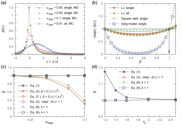
Figure 1: (a) The distributions of the potential-energy change $\varepsilon$. (b) The intersection of $\exp(-\beta\varepsilon)$ and 1.0 gives the correct $\beta$. (c) The temperature versus the perturbation amplitude $u_{\max}$. (d) The temperature versus the potential cutoff $r_{c}$.

IV Numerical results

We show some results for the temperature formulas. We use Eqs. (4), (8) or (9), etc., in an MC/MD simulation in this way: once every few steps along the trajectory, we perturb the current configuration $\mathbf{q}$ by a random $\mathbf{u}$ (which is conducted as a virtual displacement so as not to disturb the real trajectory), and register the resulting change $\varepsilon=U(\mathbf{q}+\mathbf{u})-U(\mathbf{q})$ in the potential energy; the formulas then estimate the temperature $\beta$ from the accumulated distribution $p(\varepsilon)$. For the Ising model, $\mathbf{q}$ is a spin configuration, and $+\mathbf{u}$ means to flip a random spin.

IV.1 Canonical and microcanonical ensembles

Four $\varepsilon$-distributions $p(\varepsilon)$ from simulations on the 108-particle Lennard-Jones (LJ) fluid at $\rho=0.7$ and $\beta_{0}=1.0$ are shown in Fig. 1(a). The first simulation used a regular MD (in the microcanonical-like ensemble), while the others used the Metropolis MC (in the canonical ensemble). The pair potential was switched smoothly from the standard form $u(r)=4\myeps_{LJ}[(\sigma_{\mathrm{LJ}}/r)^{12}-(\sigma_{\mathrm{LJ}}/r)^{6}]$ ($\myeps_{\mathrm{LJ}}=\sigma_{\mathrm{LJ}}=1$) at $r_{s}=2.0$ to a 7th order polynomial zhang that vanishes at $r_{c}=2.5$ to avoid artifacts. In the first three cases, each coordinate of a random particle was displaced by a random number in $(-u_{\max},u_{\max})$, with $u_{\max}=0.05$ (the first two cases) or 0.1 (the third). In the last case, the perturbation was applied to all particles with $u_{\max}=0.01$. The number of perturbations was $10^{7}$ in each case. Eqs. (8) and (9) were adapted to the MD or canonical ensemble in the sense of $\langle\dots\rangle_{U}\rightarrow\langle\dots\rangle$. A comparison of the first two cases shows that the distribution was not very sensitive to the ensemble type in this case. The distributions from the single-particle perturbations peaked at $\varepsilon=0$ [cf. Eq. (29)]. The distribution from the all-particle perturbation, however, was Gaussian-like [cf. Eq. (30)]. The integral relations applied to all cases, e.g., the $\beta$ given by Eq. (3) were 1.0077, 0.9990, 1.0160, and 0.9997, respectively.

The solution process of Eq. (3) is illustrated in Fig. 1(b): if we plot $\langle\exp(-\beta\varepsilon)\rangle$ against $\beta$, its intersection with 1.0 then gives the desired $\beta$. Three systems, the LJ fluid (with both single- and all-particle perturbations), square-well allen fluid and $32\times 32$ Ising model were simulated in the canonical ensemble at $\beta_{0}=1.0$ using the Metropolis algorithm. The square-well potential of two particles is infinity if their distance $r<r_{a}$, or $-\myeps_{\mathrm{sq}}$ if $r_{a}\leq r<r_{b}$, or 0 otherwise ($r_{a}=1$, $r_{b}=1.5$, and $\myeps_{\mathrm{sq}}=1$). Perturbations that produced clashes, hence infinite $\varepsilon$, were excluded from entering Eq. (3).

In Fig. 1(c), the temperatures computed from Eqs. (1)-($\ref{eq:canon}^{\prime}$), (8) and (9), were plotted against $u_{\max}$, the size of the single-particle perturbation. All formulas worked well with a small $u_{\max}$, but with a large $u_{\max}$, Eq. (2) and ($\ref{eq:canon}^{\prime}$) quickly lost accuracy, while the integral formulas were little affected.

The effect of the potential truncation butler was studied using a set of MC simulations ($u_{\max}=0.05$) with the LJ potential deliberately truncated at small $r_{c}$. The discontinuity rendered Eq. (1) approximate butler . As shown in Fig. 1(d), a small $r_{c}$ indeed affected Eq. (1), but not Eqs. (3), (8), and (9).

IV.2 Constant potential-energy ensemble

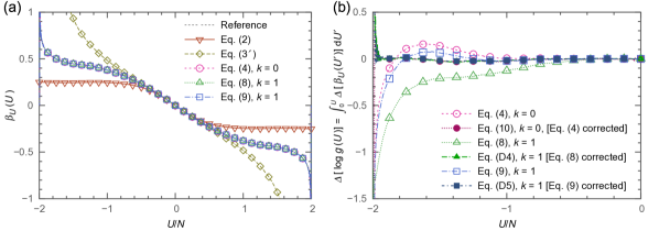
Figure 2: (a) The profile of the temperature of potential energy $\beta_{U}(U)$ along $U$ in the $32\times 32$ Ising model. (b) The error of $\log g(U)=\int_{0}^{U}\beta_{U}(U^{\prime})\,dU^{\prime}$. The reference values $\beta_{U}^{*}(U)$ were computed as $[\log g^{*}(U+\Delta U)-\log g^{*}(U-\Delta U)]/(2\Delta U)$ with $\Delta U=4$.

The temperature profile $\beta_{U}(U)$ along the potential energy was computed on the $32\times 32$ Ising model. To cover the entire energy range, we ran a multicanonical simulation yan ; multicanonical using the exact density of states $g^{*}(U)$ beale in the sampling weight for $10^{7}$ MC steps per site. As shown in Fig. 2(a), the temperature from Eqs. (2) and ($\ref{eq:canon}^{\prime}$) behaved badly except around $U\approx 0$ or $\beta_{U}\approx 0$, while the integral relations (4), (8) and (9) agreed with the reference $\beta^{*}(U)$. This is expected, as the smallest energy change is 4 in the system, $\beta\,\varepsilon\ll 1$ rarely holds, while $\varepsilon$ is still $O(1)$ to justify the use of the integral relations. But even in the latter case, there was an $O(1)$ difference between the integral $\log g(U)=\int^{U}\beta_{U}(U^{\prime})\,dU^{\prime}$ and the exact $\log g^{*}(U)$ [Fig. 2(b)], showing that the temperature from Eqs. (4), (8) and (9) had an $O(1/N)$ systematic error without the corrections, as the entire potential-energy range was $O(N)$. The corrections (10), (34) and (35), however, effectively removed the remaining errors (except around the ground states, where the density of states was intrinsically irregular).

IV.3 Temperature matching

As an application, Eq. (3) can be used to help a simplified potential-energy function emulate a more complex or realistic one coarsegrain ; forcematching ; shell . In the following example, the simplified function is the hard-sphere potential $U_{\mathrm{hs}}(\mathbf{q})$, and the more realistic one is the LJ potential $U_{\mathrm{LJ}}(\mathbf{q})$. We first run a simulation using $U_{\mathrm{hs}}$ as the potential energy. From the trajectory, we evaluate the effective temperature $\beta_{\mathrm{LJ}}$, by seeking the solution of $\langle e^{-\beta_{\mathrm{LJ}}\Delta U_{\mathrm{LJ}}}\rangle_{\mathrm{hs}}=1$, with $\Delta U_{\mathrm{LJ}}$ being the change caused by a virtual perturbation. We repeat the process with a modified $U_{\mathrm{hs}}$ until the $\beta_{\mathrm{LJ}}$ matches the simulation temperature $\beta$:

$$\langle e^{-\beta_{\mathrm{LJ}}\,\Delta U_{\mathrm{LJ}}}\rangle_{\mathrm{hs}}=1.$$ (19)

Thus, Eq. (19) calibrates the hard-sphere system by the virtual thermometer gauged in the LJ system (cf. Appendix F).

Similar to Eq. (19), one can also match the potential energy as $\langle U_{\mathrm{LJ}}\rangle_{\mathrm{hs}}=\langle U_{\mathrm{LJ}}\rangle_{\mathrm{LJ}}$ or pressure as $\langle p_{\mathrm{LJ}}\rangle_{\mathrm{hs}}=\langle p_{\mathrm{LJ}}\rangle_{\mathrm{LJ}}$. Another alternative is to minimize the relative entropy hansen ; shell ; gbproof

$$S_{r}=\int\log[w_{\mathrm{hs}}(\mathbf{q})/w_{\mathrm{LJ}}(\mathbf{q})]w_{\mathrm{hs}}(\mathbf{q})\,d\mathbf{q},$$ (20)

which measures the difference between the distributions $w_{\mathrm{LJ}}=e^{-\beta U_{\mathrm{LJ}}}/Z_{\mathrm{LJ}}$ and $w_{\mathrm{hs}}=e^{-\beta U_{\mathrm{hs}}}/Z_{\mathrm{hs}}$. Although Eq. (19) and the conditions of matching the potential energy and pressure can all be derived from minimizing $S_{r}$ regarding virtual variations hansen ; shell ; gbproof of $w_{\mathrm{LJ}}$ (Appendix F), they do not necessarily find the exact optimal $U_{\mathrm{hs}}$ that minimizes $S_{r}$.

The methods were tested on a fluid system of 108 particles. The diameter $r_{a}$ of the hard-sphere system was varied to match the LJ system under three conditions. The ratio of the partition functions $Z_{\mathrm{LJ}}/Z_{\mathrm{hs}}$, required for computing $S_{r}$, were obtained by Bennett’s acceptance ratio method bennett from independent simulations on the two systems. Table 1 shows that the obtained $r_{a}$ from the above methods were generally close in the gaseous phase. It was, however, not always possible to find solutions for all methods, e.g., matching the potential energy failed in the second case, while the relative entropy was hard to compute in the third case. Thus, the methods can be complementary. Like the force-matching method forcematching , the temperature matching requires simulation in only one (hard-sphere) system. One may also treat the configuration temperature as a special thermal force, and thus add a restraint to the force-matching method. Also note that Eq. (19) allows a local perturbation with cheap local energy calculations.

Table 1: Matching of the hard-sphere and Lennard-Jones systems.

$r_{a}^{\dagger}$	$S_{r}(k_{B})^{\ddagger}$	$\beta_{\mathrm{LJ}}^{\P}$	$\langle U_{\mathrm{LJ}}\rangle_{\mathrm{hs}}^{\S}$	$\langle U_{\mathrm{LJ}}\rangle_{\mathrm{LJ}}^{\S}$	$\langle p_{\mathrm{LJ}}\rangle_{\mathrm{hs}}^{\S}$	$\langle p_{\mathrm{LJ}}\rangle_{\mathrm{LJ}}^{\S}$
I. $T=2.5$, $\rho=0.3$
0.900	15.2	0.24	$-1.25$	$-1.82$	1.620	0.728
0.952	7.1	0.62	$-1.73$	$-1.82$	0.729	0.729
0.970	8.4	0.86	$\mathbf{-1.82}$	$\mathbf{-1.82}$	0.532	0.728
0.978	9.4	1.00	$-1.84$	$-1.82$	0.459	0.727
1.000	13.6	1.52	$-1.90$	$-1.82$	0.289	0.728
II. $T=1.0$, $\rho=0.05$
0.900	13.4	0.23	$-0.21$	$-0.47$	0.065	0.036
0.981	$\mathbf{8.6}$	$\mathbf{1.01}$	$-0.28$	$-0.47$	0.038	0.036
0.993	8.8	1.27	$-0.28$	$-0.47$	0.036	0.036
1.000	9.0	1.40	$-0.28$	$-0.47$	0.035	0.036
III. $T=1.0$, $\rho=0.7$
0.900	180	0.28	$-2.33$	$-4.89$	9.88	$-0.06$
0.970	37	1.00	$-4.44$	$-4.89$	1.89	$-0.05$
0.999	-	1.74	$-4.88$	$-4.90$	$\mathbf{-0.04}$	$\mathbf{-0.06}$
1.000	-	1.77	$\mathbf{-4.89}$	$\mathbf{-4.89}$	$-0.11$	$-0.06$
Each simulation took $10^{7}$ MC steps; $r_{c}=2.5$ for the LJ potential. The points of minimal entropy and matched quantities are shown in boldface.
† Diameter of hard spheres.
‡ Defined in Eq. (20).
¶ From Eq. (19) with a single-particle perturbation and $u_{\max}=0.02$.
§ Figures have been divided by the number of particles.

V Conclusions

To sum up, temperature can be extracted from the distribution $p(\varepsilon)$ of the potential-energy change $\varepsilon$ caused by configuration perturbations, as the nontrivial root of Eqs. (4), (8) or (9). The formulas can be understood as virtual thermometers gauged in a corresponding canonical ensemble. When used in the constant potential-energy ensemble, the formulas have an $O(1/N)$ error, but can be corrected systematically.

The approach can be extended to the mean force of a multidimensional distribution $\rho(\vec{X})$ by an ensemble-adjusted perturbation. The adjusted perturbation is equivalent to a short trajectory of a reversible dynamics, making the mean force formulas (15) and (17) readily usable in simulations and experiments experiments . The computer code of the examples can be found in Ref. software .

Appendix A Configuration temperature

Following Refs. rugh ; butler ; jepps , we show that the temperature $\beta_{U}=\frac{d}{dU}g(U)$ in the constant potential-energy ensemble (cf. Sec. II.3) satisfies

$$\beta_{U}=\frac{\langle\nabla\cdot\mathbf{B}\rangle_{U}}{\langle\mathbf{B}\cdot\nabla U\rangle_{U}}-\frac{d\log\langle\mathbf{B}\cdot\nabla U\rangle_{U}}{dU},$$ (21)

where $\mathbf{B}=\mathbf{B}(\mathbf{q})$ is a vector field that satisfies $\mathbf{B}\cdot\nabla U>0$ jepps . The second term on the right is $O(1/N)$. We first define jepps

$$G(U)=\int(\mathbf{B}\cdot\nabla U)\,\delta[U(\mathbf{q})-U]\,d\mathbf{q}=\langle\mathbf{B}\cdot\nabla U\rangle_{U}\,g(U).$$

Then

$$\frac{dG}{dU}=\left(\frac{d\langle\mathbf{B}\cdot\nabla U\rangle_{U}}{dU}+\langle\mathbf{B}\cdot\nabla U\rangle_{U}\beta_{U}\right)g(U).$$ (22)

On the other hand, integration by parts yields

$$\frac{dG}{dU} =-\int\mathbf{B}\cdot\nabla\delta[U(\mathbf{q})-U]d\mathbf{q}$$

$$=\int(\nabla\cdot\mathbf{B})\delta[U(\mathbf{q})-U]d\mathbf{q}=\langle\nabla\cdot\mathbf{B}\rangle_{U}g(U).$$ (23)

Equating Eqs. (22) and (23) gives (21). Eq. (1) represents two special cases. With $\mathbf{B}=\nabla U/(\nabla U\cdot\nabla U)$, $\mathbf{B}\cdot\nabla U=1$, and

$$\beta_{U} =\left\langle\frac{\nabla U}{\nabla U\cdot\nabla U}\right\rangle_{U}-\left\langle\frac{2\nabla U\cdot\nabla\nabla U\cdot\nabla U}{(\nabla U\cdot\nabla U)^{2}}\right\rangle_{U},$$ (24)

where the second term is $O(1/N)$. With $\mathbf{B}=\nabla U$, we get

$$\beta_{U}=\frac{\langle\nabla^{2}U\rangle_{U}}{\langle\nabla U\cdot\nabla U\rangle_{U}}-\frac{d\log\langle\nabla U\cdot\nabla U\rangle_{U}}{dU}.$$ (25)

We can show Eq. (1) from the equation of motion darve2008 ; hansen :

$$\langle\mathbf{B}\cdot\nabla U\rangle =\frac{1}{\tau}\int_{0}^{\tau}(\mathbf{B}\cdot\nabla U)\,dt=-\frac{1}{\tau}\int_{0}^{\tau}(\mathbf{B}\cdot\dot{\mathbf{p}})\,dt$$

$$=\frac{1}{\tau}\int_{0}^{\tau}(\mathbf{p}\cdot\dot{\mathbf{B}})\,dt=\frac{1}{\tau}\int_{0}^{\tau}(\mathbf{p}\cdot\nabla\mathbf{B}\cdot\dot{\mathbf{q}})\,dt$$

$$=\langle\mathbf{p}\cdot\nabla\mathbf{B}\cdot\mathbf{p}/m\rangle\approx k_{B}T\langle\nabla\cdot\mathbf{B}\rangle,$$

where $\tau$ is the length of a long trajectory. We have assumed a thermostat hoover ; thermostat2 that makes momenta $\mathbf{p}$ independent: $\langle p_{i}p_{j}/m\rangle=k_{B}T\delta_{ij}$, and uncorrelated with $\mathbf{B}$ and $\nabla\mathbf{B}$. This derivation has the advantage of replacing the strong assumption of global ergodicity in the ensemble theory by a weaker condition of sufficiently randomized momenta (which requires only local equilibration).

Appendix B Fluctuation theorems

Eq. (3) can be generalized by several fluctuation theorems maes ; bkfluc ; fluc ; jarzynski ; kurchan ; seifert2005 . For any $\beta^{\prime}$, we have

$$\langle\exp[(\beta^{\prime}-\beta)\,\varepsilon]\rangle_{\beta}=\langle\exp(-\beta^{\prime}\varepsilon^{*})\rangle_{\beta},$$

where $\varepsilon$ and $\varepsilon^{*}$ are the energy changes caused by a pair of uniform perturbations $+\mathbf{u}$ and $-\mathbf{u}$, respectively maes , because

$$\int e^{(\beta^{\prime}-\beta)\,[U(\mathbf{q}+\mathbf{u})-U(\mathbf{q})]}\,e^{-\beta U(\mathbf{q})}/Z(\beta)\,d\mathbf{q}$$

$$=\int e^{-\beta^{\prime}\,[U(\mathbf{q}^{\prime}-\mathbf{u})-U(\mathbf{q}^{\prime})]}\,e^{-\beta U(\mathbf{q}^{\prime})}/Z(\beta)\,d\mathbf{q}^{\prime},$$

where $\mathbf{q}^{\prime}=\mathbf{q}+\mathbf{u}$. For a symmetrically randomized perturbation, the distributions of $\varepsilon$ and $\varepsilon^{*}$ are identical, and

$$\langle\exp[(\beta^{\prime}-\beta)\,\varepsilon]\rangle_{\beta}=\langle\exp(-\beta^{\prime}\varepsilon)\rangle_{\beta}.$$ (26)

The $\varepsilon$ distribution can be found from the exponential average $g(i\omega)\equiv\langle\exp(-i\omega\varepsilon)\rangle_{\beta}$ vankampen as $p(\varepsilon)=\frac{1}{2\pi}\int_{-\infty}^{\infty}g(i\omega)\,e^{i\omega\varepsilon}\,d\omega$. By taking the Fourier transform of Eq. (26), we get

$$p(\varepsilon)\,\exp(-\beta\varepsilon)=p(-\varepsilon),$$ (27)

assuming that $g(i\omega)$ has no singularity in the strip $0<\mathrm{Re}\,(i\omega)<\beta$ of the complex plane. Note that while Eqs. (26) and (27) require a symmetric perturbation, Eq. (3) does not.

Eq. (3) has a few other generalizations. For a Hamiltonian $H_{\lambda}(\mathbf{q})$ parameterized by $\lambda$, we can treat a circular switch of $\lambda:0\rightarrow 1\rightarrow 0$ starting from the canonical equilibrium state at $\lambda=0$ as an elaborate perturbation. Then the Jarzynski equality states $\langle\exp(-\beta W)\rangle=1$ for the non-equilibrium work $W=\int_{0}^{\tau}(\partial H_{\lambda}/\partial\lambda)\,\dot{\lambda}\,dt$ over a period $\tau$ jarzynski . Similarly, we have $\langle\exp(-\beta\tilde{W})\rangle=1$ for the work $\tilde{W}=\int_{0}^{\tau}\mathbf{f}(\mathbf{q},t)\cdot\dot{\mathbf{q}}\,dt$ derived from a time-dependent driving force $\mathbf{f}(\mathbf{q},t)$ (excluding the component from the conservative potential) bkfluc ; seifert2008 . These relations can also be used to extract the equilibrium temperature $\beta$ of the initial equilibrium state.

Appendix C Harmonic oscillator

We verify a few formulas for the canonical ensemble on a $D$-dimensional harmonic oscillator with the potential energy $U(\mathbf{q})=\frac{1}{2}k\mathbf{q}^{2}$. For a Gaussian perturbation $p_{\mathbf{u}}(\mathbf{u})\propto\exp(-\mathbf{u}^{2}/2\sigma^{2})$ applied to a fixed $\mathbf{q}$, the average

$$g_{\mathbf{q}}(b) \equiv\overline{\exp(-b\,\varepsilon)}=\int e^{-b[U(\mathbf{q}+\mathbf{u})-U(\mathbf{q})]}p_{\mathbf{u}}(\mathbf{u})\,d\mathbf{u}$$

$$=(1+\alpha b)^{-D/2}\exp[\alpha b^{2}U/(1+\alpha b)],$$

where $\alpha=k\sigma^{2}$. Averaging $g_{\mathbf{q}}(b)$ over $\mathbf{q}$ yields

$$g(b) \equiv\langle g_{\mathbf{q}}(b)\rangle_{\beta}=\int g_{\mathbf{q}}(b)\,e^{-\beta U(\mathbf{q})}/Z(\beta)\,d\mathbf{q}$$

$$=[1+\alpha b(1-b/\beta)]^{-D/2}.$$ (28)

Eq. (28) satisfies Eqs. (3) and (26), i.e., $g(\beta^{\prime})=g(\beta-\beta^{\prime})$.

Since $g(b)$ gives the moment generating function vankampen , the $\varepsilon$ distribution $p(\varepsilon)=\frac{1}{2\pi}\int_{-\infty}^{+\infty}g(i\omega)e^{i\omega\varepsilon}\,d\omega$ is

$$p(\varepsilon)=\dfrac{[|\varepsilon|/(2\gamma)]^{(D-1)/2}}{(\alpha/\beta)^{D/2}}\dfrac{K_{(D-1)/2}(\gamma|\varepsilon|)}{\sqrt{\pi}\Gamma(D/2)}e^{\beta\varepsilon/2},$$ (29)

where $\gamma=\sqrt{(\beta/2)^{2}+(\beta/\alpha)}$, $K_{n}(x)$ is the modified Bessel function of the second kind, and $\Gamma(x)$ is the gamma function. Eq. (29) satisfies Eq. (27), and shows that $p(\varepsilon)$ at $\varepsilon=0$ depends critically on the dimension $D$: it diverges if $D<2$; it has a finite cusp if $D=2$; and it is differentiable if $D>2$. In the limit of $D\gg 1$ and $\alpha\beta\ll 1$, the distribution is Gaussian:

$$p(\varepsilon)\approx\big{(}1/\sqrt{2\pi\sigma^{2}}\big{)}\exp\big{[}-(\varepsilon-\alpha D/2)^{2}/(2\sigma^{2})\big{]},$$ (30)

where $\sigma^{2}=(\alpha/\beta+\alpha^{2}/2)D\approx(\alpha/\beta)D$.

Appendix D Series expansion

We derive the corrections for Eqs. (4), (8) and (9) from

$$p_{U}(-\varepsilon) =\dfrac{g(U-\varepsilon)}{g(U)}p_{U-\varepsilon}(+\varepsilon)$$

$$=\exp\left[\sum_{l=1}^{\infty}\dfrac{b_{l}(-\varepsilon)^{l}}{l!}\right]\sum_{m=0}^{+\infty}\dfrac{(-\varepsilon)^{m}}{m!}\dfrac{d^{m}p_{U}(\varepsilon)}{dU^{m}},$$ (31)

where $b_{l}=\frac{d^{l}}{dU^{l}}\log g(U)$. Eq. (4) seeks the root $\hat{\beta}$ of

$$0=\int_{-\infty}^{+\infty}\left[p_{U}(-\varepsilon)\,e^{\hat{\beta}\,\varepsilon}-p_{U}(\varepsilon)\right]\,\varepsilon^{k}\,d\varepsilon.$$

Using Eq. (31) for $p_{U}(-\varepsilon)$ yields:

$$\langle\varepsilon^{k}\rangle_{U}=\sum_{m=0}^{\infty}\tfrac{(-)^{m}}{m!}\tfrac{\bar{d}^{m}}{\bar{d}U^{m}}\left\langle\exp\left[\hat{\beta}\varepsilon+\textstyle\sum_{l}\tfrac{b_{l}(-\varepsilon)^{l}}{l!}\right]\varepsilon^{k+m}\right\rangle_{U},$$ (32)

where $\bar{d}^{m}/\bar{d}U^{m}$ denotes a differentiation that applies only to the moments of $\varepsilon$, but not to the $\hat{\beta}$ or $b_{l}$.

Eq. (32) can be solved by successive approximations: $\hat{\beta}=\hat{\beta}^{(1)}+\hat{\beta}^{(2)}+\dots$ with $\hat{\beta}^{(n)}\sim O(1/{N^{n-1}})$. To the first order, we use $\hat{\beta}=\hat{\beta}^{(1)}$ in Eq. (32), and

$$\langle\varepsilon^{k}\rangle_{U}\approx\langle\exp(\hat{\beta}^{(1)}\varepsilon-b_{1}\varepsilon)\varepsilon^{k}\rangle_{U},$$

which yields $\hat{\beta}^{(1)}=b_{1}$. Next, we set $\hat{\beta}=\hat{\beta}^{(1)}+\beta^{(2)}$, and

$$\left\langle\varepsilon^{k}\right\rangle_{U} \approx\left\langle\exp\left(\hat{\beta}^{(2)}\varepsilon+\tfrac{1}{2}b_{2}\varepsilon\right)\varepsilon^{k}\right\rangle_{U}-\tfrac{d}{dU}\left\langle\varepsilon^{k+1}\right\rangle_{U},$$

which yields $\hat{\beta}^{(2)}=\left[-\frac{1}{2}\,b_{2}\langle\varepsilon^{k+2}\rangle_{U}+\frac{d}{dU}\langle\varepsilon^{k+1}\rangle_{U}\right]/{\langle\varepsilon^{k+1}\rangle_{U}}$. We reach Eq. (10) by $d\beta_{U}/dU\approx d\hat{\beta}/dU$.

Eq. (10) is exact for any $N$ in the limit of small $\varepsilon$. For an even $k$ in this limit, it becomes (cf. Sec. II.1)

$$\beta_{U}=\dfrac{2\langle\varepsilon^{k+1}\rangle_{U}}{\langle\varepsilon^{k+2}\rangle_{U}}-\dfrac{d\log\langle\varepsilon^{k+2}\rangle_{U}}{dU},$$ (33)

with $\hat{\beta}=2\langle\varepsilon^{k+1}\rangle_{U}/\langle\varepsilon^{k+2}\rangle_{U}$. To show this, we use

$$\,\langle\varepsilon^{k+2}\rangle_{U} =\textstyle\sum_{\{i\}}\langle\partial_{i_{1}}U\cdots\partial_{i_{k+2}}U\rangle_{U}\,\overline{u_{i_{1}}\cdots u_{i_{k+2}}},$$

$$2\langle\varepsilon^{k+1}\rangle_{U} =(k+1)\textstyle\sum_{\{i\}}\langle\partial_{i_{1}}U\dots\partial_{i_{k}}U\partial_{i_{k+1}i_{k+2}}^{2}U\rangle_{U}\,\overline{u_{i_{1}}\dots u_{i_{k+2}}}.$$

Partial integration yields $\frac{d}{dU}[\langle\varepsilon^{k+2}\rangle_{U}\,g(U)]=2\langle\varepsilon^{k+1}\rangle_{U}\,g(U)$, which is Eq. (33). For an odd $k$, the $\beta_{U}$ value is identical to that from the $k-1$ case in the small $\varepsilon$ limit.

The correction for Eq. (8) can be constructed from

$$0=\int_{-\infty}^{\infty}\mathrm{sgn}(\varepsilon)|\varepsilon|^{k}\min\left\{1,e^{-\hat{\beta}\,\varepsilon}\right\}\left[p_{U}(-\varepsilon)\,e^{\hat{\beta}\,\varepsilon}-p_{U}(\varepsilon)\right]\,d\varepsilon.$$

Using Eq. (31) for $p_{U}(\varepsilon)$ yields

$$\beta_{U}\approx\hat{\beta}-\dfrac{m_{k+2}}{2\,m_{k+1}}\dfrac{d|\hat{\beta}|}{dU}-\dfrac{d\log m_{k+1}}{dU},$$ (34)

where $m_{l}\equiv\int_{-\infty}^{+\infty}|\varepsilon|^{l}\min\{1,\exp(-\hat{\beta}\,\varepsilon)\}p(\varepsilon)\,d\varepsilon$. To correct the $\hat{\beta}$ value determined from Eq. (9), we use

$$0=\int_{-\infty}^{\infty}\mathrm{sgn}(\varepsilon)|\varepsilon|^{k}e^{-\hat{\beta}\varepsilon/2}\left[p_{U}(-\varepsilon)\,e^{\hat{\beta}\varepsilon}-p_{U}(\varepsilon)\right]\,d\varepsilon,$$

which yields

$$\beta_{U}\approx\hat{\beta}-\dfrac{d}{dU}\log\left\langle|\varepsilon|^{k+1}\exp\left(-\dfrac{1}{2}\hat{\beta}\varepsilon\right)\right\rangle_{U},$$ (35)

Eq. (35) lacks the $d\hat{\beta}/dU$ term in Eqs. (10) and (34), as it has been included in differentiating the $\hat{\beta}$ in the $\exp(-\frac{1}{2}\hat{\beta}\,\varepsilon)$.

Appendix E Distribution mean force

For the $K$-dimensional distribution rugh ; meanforce ; bluemoon ; darve2008 ; zhang $\rho(\vec{X})$ defined by Eq. (16), we have

$$f_{\alpha}\equiv\frac{\partial\log\rho}{\partial X_{\alpha}}=\sum_{\gamma}(\overset{\leftrightarrow}{W}^{-1})_{\alpha\gamma}\left(F_{\gamma}-\sum_{\theta}\dfrac{\partial W_{\gamma\theta}}{\partial X_{\theta}}\right).$$ (36)

where $\overset{\leftrightarrow}{W}$ is the $K$ by $K$ matrix with $W_{\alpha\gamma}(\vec{X})\equiv\langle\mathbf{B}_{\alpha}\cdot\nabla X_{\gamma}\rangle_{\vec{X}}$ (the $\mathbf{B}_{\alpha}$ are vector fields such that the matrix has an inverse ${\overset{\leftrightarrow}{W}}^{-1}$), and $F_{\alpha}\equiv\langle\nabla\cdot\mathbf{B}_{\alpha}+\mathbf{B}_{\alpha}\cdot\nabla\log w\rangle_{\vec{X}}.$ Particularly, if $K=1$,

$$\frac{d\log\rho}{dX}=\frac{\langle\nabla\cdot\mathbf{B}+\mathbf{B}\cdot\nabla\log w\rangle_{X}}{\langle\mathbf{B}\cdot\nabla X\rangle_{X}}-\frac{d\log\langle\mathbf{B}\cdot\nabla X\rangle_{X}}{dX}.$$

which is similar to Eq. (21). To show Eq. (36), we observe

$$W_{\alpha\gamma}\,\rho=\int(\mathbf{B}_{\alpha}\cdot\nabla X_{\gamma})\,\textstyle\prod_{\gamma}\delta[X_{\gamma}(\mathbf{q})-X_{\gamma}]w(\mathbf{q})\,d\mathbf{q}.$$

Then partial integration gives

$$F_{\alpha}\rho =\int\nabla\cdot[w(\mathbf{q})\,\mathbf{B}_{\alpha}]\,\textstyle\prod_{\gamma}\delta[X_{\gamma}(\mathbf{q})-X_{\gamma}]\,d\mathbf{q}$$

$$=\textstyle\sum_{\gamma}\partial{(W_{\alpha\gamma}\,\rho)}/{\partial X_{\gamma}}=\textstyle\sum_{\gamma}\left(W_{\alpha\gamma}f_{\gamma}+\partial{W_{\alpha\gamma}}/{\partial X_{\gamma}}\right)\,\rho.$$

Multiplying $\overset{\leftrightarrow}{W}^{-1}$ to both sides yields Eq. (36).

If $\mathbf{B}_{\alpha}$ is constructed by the Gram-Schmidt orthonormalization such that $W_{\alpha\gamma}=\langle\mathbf{B}_{\alpha}\cdot\nabla X_{\gamma}\rangle_{\vec{X}}=\delta_{\alpha\gamma}$ rugh ; bluemoon , then

$$f_{\alpha}=F_{\alpha}=\langle\nabla\cdot\mathbf{B}_{\alpha}+\mathbf{B}_{\alpha}\cdot\nabla\log w\rangle_{\vec{X}}.$$

The resulting $\nabla\cdot\mathbf{B}_{\alpha}$ can be quite complex henin , e.g., for $K=2$,

$$\mathbf{B}_{\alpha}=\frac{\textstyle\sum_{\mu=1,2}\nabla X_{\mu}\cdot\nabla X_{\mu}-\nabla X_{\mu}\otimes\nabla X_{\mu}}{(\nabla X_{1}\cdot\nabla X_{1})(\nabla X_{2}\cdot\nabla X_{2})-(\nabla X_{1}\cdot\nabla X_{2})^{2}}\,\nabla X_{\alpha}.$$

We can alternatively set $\mathbf{B}_{\alpha}=\nabla X_{\alpha}$, and

$$\begin{split}W_{\alpha\gamma}(\vec{X})&=\langle\nabla X_{\alpha}\cdot\nabla X_{\gamma}\rangle_{\vec{X}},\\ F_{\alpha}&=\langle\nabla^{2}X_{\alpha}+\nabla X_{\alpha}\cdot\nabla\log w\rangle_{\vec{X}},\end{split}$$ (37)

which limits the second derivatives to the Laplacians, but requires the corrections $\frac{\partial}{\partial X_{\theta}}W_{\gamma\theta}$ from numerical differentiation.

Appendix F Relative entropy

We show below that the temperature matching condition Eq. (19) locally minimizes the relative entropy shell

$$S_{r}^{*}=-\int\log\left[\frac{w_{A}(\mathbf{q}^{\prime})}{w_{B}(\mathbf{q})}\left|\frac{\partial\mathbf{q}^{\prime}}{\partial\mathbf{q}}\right|\right]\,w_{B}(\mathbf{q})\,d\mathbf{q},$$

of two distributions $w_{A}(\mathbf{q})$ and $w_{B}(\mathbf{q})$ ($A\rightarrow\mathrm{LJ},B\rightarrow\mathrm{hs}$) along the force. If $\mathbf{q}^{\prime}=\mathbf{q}$, the minimum is located at $w_{A}=w_{B}$ [use $-\log x\geq 1-x$ with $x=w_{A}/w_{B}$ hansen ; shell ; gbproof ]. If, however, $S_{r}^{*}$ is minimized along an infinitesimal coordinate transformation $\mathbf{q}^{\prime}=\mathbf{q}+\delta\lambda\mathbf{B}(\mathbf{q})$, then $\partial S_{r}^{*}/\partial(\delta\lambda)=0$, or $\langle\nabla\cdot\mathbf{B}+\mathbf{B}\cdot\nabla\log w_{A}\rangle_{B}=0$. In the canonical ensemble,

$$\beta_{A}=\left\langle\nabla\cdot\mathbf{B}\right\rangle_{B}/\left\langle\mathbf{B}\cdot\nabla U_{A}\right\rangle_{B},$$ (38)

for $w_{A}(\mathbf{q}^{\prime})\propto\exp[-\beta_{A}U_{A}(\mathbf{q}^{\prime})]$. Particularly, with $\mathbf{B}=\nabla U_{A}$, we have $\beta_{A}=\langle\nabla^{2}U_{A}\rangle_{B}/\langle\nabla U_{A}\cdot\nabla U_{A}\rangle_{B}$, which is Eq. (19) in the small-perturbation limit. Generally, Eq. (38) defines a distinct effective temperature $\beta_{A}$ for each vector field $\mathbf{B}$, reflecting the fact that one can define different effective temperatures casas in a non-equilibrium state ($w_{A}$: equilibrium, $w_{B}$: non-equilibrium). The conditions for matching the potential energy and pressure can be similarly obtained by varying $w_{A}$ with respect to the temperature and volume, respectively.

Normally, we set $w_{A}$ as the model distribution, and optimize its parameters to match the reference $w_{B}$ shell ; thus, the averages should be performed in the reference $B$ system. This is, however, inconvenient, for the example in Sec. IV.3, since $\log w_{\mathrm{hs}}$, when averaged over configurations produced by the reference LJ potential, can be infinite, due to the hard-sphere potential $U_{B}$. We therefore set $A\rightarrow\mathrm{LJ}$ and $B\rightarrow\mathrm{hs}$.

Appendix G Driven Langevin system

We use a driven system in constant contact with a heat bath as a model to study the temperature in a non-equilibrium steady state. We will show below that, to correctly extract the presumably constant heat bath temperature, Eq. (3) should be applied to a nonuniform perturbation.

Consider the overdamped Langevin equation kurchan ; seifert2005 : $d\mathbf{q}/dt=\mathbf{F}/\eta+\sqrt{2/(\beta\eta)}\xi$, where the total force $\mathbf{F}$ is the conservative component $-\nabla U$ plus a driving $\mathbf{f}$, $\eta$ is the viscosity, and $\xi$ is a Gaussian white noise satisfying $\langle\xi_{i}(t)\xi_{j}(t^{\prime})\rangle=\delta_{ij}\delta(t-t^{\prime})$. The steady-state distribution $w$ satisfies

$$\nabla\log w=\beta\mathbf{F}-\beta\eta\mathbf{j}/w,$$ (39)

where $\mathbf{j}$ is the constant current, and the ratio $\mathbf{v}=\mathbf{j}/w$ is the average local velocity seifert2005 . The equilibrium case $w\propto\exp(-\beta U)$ is recovered if $\mathbf{f}=\mathbf{j}=\mathbf{0}$.

Consider a perturbation $\mathbf{q}\rightarrow\mathbf{q}^{\prime}$ generated by a flow from the vector field $\mathbf{u}(\mathbf{q})$, $d\mathbf{q}/d\tau=\mathbf{u}[\mathbf{q}(\tau)]$, over a period of “virtual time” $\tau_{m}$, such that $\mathbf{q}(\tau=0)=\mathbf{q}$ and $\mathbf{q}(\tau=\tau_{m})=\mathbf{q}^{\prime}$. We then have, by Eq. (39),

$$\left\langle e^{-\beta\varepsilon_{\mathrm{eff}}-\beta q_{\mathrm{hk}}}\,J\right\rangle=\int\frac{w(\mathbf{q}^{\prime})}{w(\mathbf{q})}\left|\frac{\partial\mathbf{q}^{\prime}}{\partial\mathbf{q}}\right|w(\mathbf{q})\,d\mathbf{q}=1,$$ (40)

where $\varepsilon_{\mathrm{eff}}\equiv-\int_{0}^{\tau_{m}}\mathbf{F}[\mathbf{q}(\tau)]\cdot\mathbf{u}[\mathbf{q}(\tau)]\,d\tau$ is the change of the local effective potential reimann or the absorbed heat, $q_{\mathrm{hk}}\equiv\int_{0}^{\tau_{m}}\eta\mathbf{u}[\mathbf{q}(\tau)]\cdot\mathbf{v}[\mathbf{q}(\tau)]\,d\tau$ is the housekeeping heat kurchan ; seifert2005 ; oono , and $J\equiv\exp\left(\int_{0}^{\tau_{m}}\nabla\cdot\mathbf{u}[\mathbf{q}(\tau)]\,d\tau\right)=|\partial\mathbf{q}^{\prime}/\partial\mathbf{q}|$ seifert2008 .

Eq. (40) can be made to locally resemble the equilibrium version [Eq. (3)] as $\left\langle\exp(-\beta\varepsilon_{\mathrm{eff}})\right\rangle=1$ by a constraint $\exp(-\beta q_{\mathrm{hk}})J=1$. The constraint can be satisfied by the vector field $\mathbf{u}=\mathbf{u}_{0}\sigma(\mathbf{q})$, where $\mathbf{u}_{0}$ is a constant and $\sigma(\mathbf{q})$ satisfies $\nabla\log\sigma(\mathbf{q})=\beta\eta\mathbf{v}(\mathbf{q})$. The $\sigma(\mathbf{q})$ induces a nonuniform perturbation in the steady state with nonzero current. In this way, we get an energy-based reading of the temperature in the non-equilibrium steady state, just as in the equilibrium state, such that the same $\beta$ value can be obtained for perturbations of different sizes and directions. Similarly, if the perturbation is a short trajectory that follows the Langevin equation, or one that satisfies $\exp(-\beta\varepsilon_{\mathrm{eff}})\,J=1$, then $\langle\exp(-\beta q_{\mathrm{hk}})\rangle=1$ speck2005 ; seifert2008 yields the same $\beta$.

References

- (1) H. H. Rugh, Phys. Rev. Lett. 78, 772 (1997); J. Phys. A 31, 7761 (1998); Phys. Rev. E 64, 055101 (2001).
- (2) B. D. Butler, G. Ayton, O. G. Jepps, and D. J. Evans, J. Chem. Phys. 109, 6519 (1998).
- (3) O. G. Jepps, G. Ayton, and D. J. Evans, Phys. Rev. E 62, 4757 (2000).
- (4) D. A. McQuarrie, Statistical Mechanics (Harper & Row, New York, 1976); S.-K. Ma, Statistical Mechanics (World Scientific, Philadelphia, 1985).
- (5) L. D. Landau and E. M. Lifshits, Statistical Physics (Pergamon Press, Oxford, 1980).
- (6) J.-P. Hansen and I. R. McDonald, Theory of Simple Liquids (Academic Press, Amsterdam, 2007).
- (7) Q. Yan and J. J. de Pablo, Phys. Rev. Lett. 90, 035701 (2003).
- (8) A. B. Adib, Phys. Rev. E 71, 056128 (2005).
- (9) C. Braga and K. P. Travisa, J. Chem. Phys. 123, 134101 (2005).
- (10) M. P. Allen and D. J. Tildesley, Computer Simulation of Liquids (Clarendon Press, Oxford, 1987).
- (11) D. Frenkel and B. Smit, Understanding Molecular Simulation: From Algorithms to Applications (Academic Press, San Diego, 2002).
- (12) F. Weinhold, J. Chem. Phys. 63, 2479 (1979).
- (13) C. Maes, J. Stat. Phys. 95, 367 (1999); J. L. Lebowitz and H. Spohn, J. Stat. Phys. 95, 333 (1999).
- (14) A. F. Voter, J. Chem. Phys. 82, 1890 (1985).
- (15) C. Jarzynski, Phys. Rev. E 65, 046122 (2002).
- (16) B. A. Berg and T. Neuhaus, Phys. Rev. Lett. 68, 9 (1992); J. Lee, Phys. Rev. Lett. 71, 211 (1993); F. G. Wang and D. P. Landau, Phys. Rev. Lett. 86, 2050 (2001); J. Kim, J. E. Straub, and T. Keyes, Phys. Rev. Lett. 97, 050601 (2006).
- (17) M. E. J. Newman and G. T. Barkema, Monte Carlo Methods in Statistical Physics (Oxford University Press, Oxford, 1999).
- (18) N. Metropolis, A. W. Rosenbluth, M. N. Rosenbluth, A. H. Teller, and E. Teller, J. Chem. Phys. 21, 1087 (1953).
- (19) V. Martin-Mayor, Phys. Rev. Lett. 98, 137207 (2007).
- (20) R. Eppenga and D. Frenkel, Mol. Phys. 52, 1303 (1984); V. I. Harismiadis, J. Vorholz, and A. Z. Panagiotopoulos, J. Chem. Phys. 105, 8469 (1996).
- (21) C. Jarzynski, Phys. Rev. Lett. 78, 2690 (1997); Phys. Rev. E 56, 5018 (1997).
- (22) H. C. Andersen, J. Chem. Phys. 72, 2384 (1980); G. J. Martyna, D. J. Tobias, and M. L. Klein, J. Chem. Phys. 101, 4177 (1994); S. Nose, J. Chem. Phys. 81, 511 (1984).
- (23) W. G. Hoover, Phys. Rev. A 31, 1695 (1985).
- (24) B. Widom, J. Chem. Phys. 39, 2808 (1963); B. Smit and D. Frenkel, Mol. Phys. 68, 951 (1989).
- (25) A. Z. Panagiotopoulos, Mol. Phys. 61, 813 (1987).
- (26) M. J. Ruiz-Montero, D. Frenkel, and J. J. Brey, Mol. Phys. 90, 925 (1997); E. Darve and A. Pohorille, J. Chem. Phys. 115, 9169 (2001).
- (27) G. Ciccotti, R. Kapral, and E. Vanden-Eijnden, Chem. Phys. Chem. 6, 1809 (2005).
- (28) E. Darve, D. Rodriguez-Gomez, and A. Pohorille, J. Chem. Phys. 128, 144120 (2008).
- (29) C. Zhang and J. Ma, J. Chem. Phys. 136, 204113 (2012).
- (30) G. M. Wang, E. M. Sevick, E. Mittag, D. J. Searles, and D. J. Evans, Phys. Rev. Lett. 89, 050601 (2002); Y. Han and D. G. Grier, Phys. Rev. Lett. 92, 148301 (2004); V. Blickle, T. Speck, L. Helden, U. Seifert, and C. Bechinger, Phys. Rev. Lett. 96, 070603 (2006); D. Andrieux, P. Gaspard, S. Ciliberto, N. Garnier, S. Joubaud, and A. Petrosyan, Phys. Rev. Lett. 98, 150601 (2007).
- (31) P. D. Beale, Phys. Rev. Lett. 76, 78 (1996).
- (32) A. P. Lyubartsev and A. Laaksonen, Phys. Rev. E 52, 3730 (1995); W. G. Noid, J.-W. Chu, G. S. Ayton, V. Krishna, S. Izvekov, G. A. Voth, A. Das, and H. C. Andersen, J. Chem. Phys. 128, 244114 (2008).
- (33) F. Ercolessi and J. B. Adams, Europhys. Lett. 26, 583 (1994); S. Izvekov, M. Parrinello, C. J. Burnham, and G. A. Voth, J. Chem. Phys. 120, 10896 (2004); S. Izvekov and G. A. Voth, J. Phys. Chem. B 109, 2469 (2005).
- (34) M. S. Shell, J. Chem. Phys. 129, 144108 (2008).
- (35) R. P. Feynman, Statistical Mechanics: A Set of Lectures (W. A. Benjamin, Reading, MA, 1972); H. B. Callen, Thermodynamics and an Introduction to Thermostatistics (Wiley, New York, 1985); P. M. Chaikin and T. C. Lubensky, Principles of Condensed Matter Physics (Cambridge University Press, Cambridge, UK, 1995).
- (36) C. H. Bennett, J. Comput. Phys. 22, 245 (1976); M. R. Shirts and J. D. Chodera, J. Chem. Phys. 129, 124105 (2008).
- (37) http://simulago.appspot.com/rpt
- (38) G. J. Martyna, M. L. Klein, and M. Tuckerman, J. Chem. Phys. 97, 2635 (1992); G. Bussi, D. Donadio, and M. Parrinello, J. Chem. Phys. 126, 014101 (2007); D. J. Evans, W. G. Hoover, B. H. Failor, B. Moran, and A. J. C. Ladd, Phys. Rev. A 28, 1016 (1983); H. Mori, Prog. Theor. Phys. 34, 399 (1965); R. Zwanzig, J. Stat. Phys. 9, 215 (1973).
- (39) G. N. Bochkov and Y. E. Kuzovlev, Physica A 106, 443 (1981).
- (40) D. J. Evans, E. G. D. Cohen, and G. P. Morriss, Phys. Rev. Lett. 71, 2401 (1993); G. Gallavotti and E. G. D. Cohen, Phys. Rev. Lett. 74, 2694 (1995); G. E. Crooks, Phys. Rev. E 60, 2721 (1999).
- (41) J. Kurchan, J. Phys. A 31, 3719 (1998); T. Hatano and S.-i. Sasa, Phys. Rev. Lett. 86, 3463 (2001).
- (42) U. Seifert, Phys. Rev. Lett. 95, 040602 (2005).
- (43) N. G. van Kampen, Stochastic Processes in Physics and Chemistry (Elsevier, Amsterdam, 2007).
- (44) U. Seifert, Eur. Phys. J. B 64, 423 (2008).
- (45) J. Hénin, G. Fiorin, C. Chipot, and M. L. Klein, J. Chem. Theory Comput. 6, 35 (2009).
- (46) J. Casas-Vázquez and D. Jou, Rep. Prog. Phys. 66, 1937 (2003); K. Martens, E. Bertin, and M. Droz, Phys. Rev. Lett. 103, 260602 (2009).
- (47) P. Reimann, Physics Reports 361, 57 (2002).
- (48) Y. Oono and M. Paniconi, Prog. Theor. Phys. Supp. 130, 29 (1998).
- (49) T. Speck and U. Seifert, J. Phys. A 38, L581 (2005).