Evolution of the Media Web

Abstract

We present a detailed study of the part of the Web related to media content, i.e., the Media Web. Using publicly available data, we analyze the evolution of incoming and outgoing links from and to media pages. Based on our observations, we propose a new class of models for the appearance of new media content on the Web where different attractiveness functions of nodes are possible including ones taken from well-known preferential attachment and fitness models. We analyze these models theoretically and empirically and show which ones realistically predict both the incoming degree distribution and the so-called recency property of the Media Web, something that existing models did not do well. Finally we compare these models by estimating the likelihood of the real-world link graph from our data set given each model and obtain that models we introduce are significantly more likely than previously proposed ones. One of the most surprising results is that in the Media Web the probability for a post to be cited is determined, most likely, by its quality rather than by its current popularity.

1 Introduction

Numerous models have been suggested to reflect and predict the growth of the Web [6, 9, 14]. The most well-known ones are preferential attachment models (see Section 2 for a more thorough discussion about previous work). One of the main drawbacks of these models is that they pay too much attention to old pages and do not realistically explain how links pointing to newly-created pages appear (as we discuss below). In this paper, we are interested in the Media Web, i.e., the highly dynamic part of the Web related to media content where a lot of new pages appear daily. We show that the Media Web has some specific properties and should therefore be analyzed separately. Note that some other parts of the Web have already been studied, for example in [17] a model for the Social Web is suggested.

Most new media pages like news and blog posts are popular only for a short period of time, i.e., such pages are mostly cited and visited for several days after they appeared [15]. We analyze this thoroughly later in the paper and introduce a recency property, which reflects the fact that new media pages tend to connect to other media pages of similar age (see Section 3).

In this context, we propose a new class of models for the appearance of new media content on the Web where different attractiveness functions of nodes are possible including ones taken from well-known preferential attachment and fitness models, but also new ones accounting for specificities of the Media Web. We analyze these models theoretically and empirically using MemeTracker public data set [1] and show which ones realistically predict both the incoming degree distribution and the recency property of the Media Web, something that existing models did not do well. Finally we compare these models by estimating the likelihood of the real-world link graph from this data set given each model and obtain that models we introduce in this paper are significantly more likely than previously proposed ones. One of the most surprising results is that in the Media Web the probability for a post to be cited is determined, most likely, by its quality rather than by its current popularity.

The contributions of this paper are the following:

• We suggest a new class of models for the appearance of new media content on the Web where different attractiveness functions of nodes are possible;

• We analyze these models theoretically and empirically and show which ones realistically depict the behavior of the Media Web;

• We compare these models by estimating the likelihood of the real-world link graph from our data set given each model.

The rest of the paper is organized as follows. In Sections 2 and 3, we discuss related work and experimental results, which motivated this work. In Section 4, based on the results of our experiments, we define our class of models. We analyze theoretically some properties of these models in Section 5, while in Section 6 we validate our models by computing the likelihood of the real-world link graph from our data given each model.

2 Related Work

One of the first attempts to propose a realistic mathematical model of the Web growth was made in [3]. The main idea is to take into account the assumption that new pages often link to old popular pages. Barabási and Albert defined a graph construction stochastic process, which is a Markov chain of graphs, governed by the preferential attachment. At each step in the process, a new node is added to the graph and is joined to $m$ different nodes already existing in the graph that are chosen with probabilities proportional to their incoming degree (the measure of popularity). This model successfully explained some properties of the Web graph like its small diameter and power law incoming degree distribution. Later, many modifications to the Barabási–Albert model have been proposed, e.g., [11, 13, 12], in order to more accurately depict these but also other properties (see [2, 7] for details).

It was noted by Bianconi and Barabási in [5] that in real networks some nodes are gaining new incoming links not only because of their incoming degree, but also because of their own intrinsic properties. For example, new Web pages containing some really popular content can acquire a large number of incoming links in a short period of time and become more popular than older pages. Motivated by this observation, Bianconi and Barabási extended preferential attachment models with pages’ inherent quality or fitness of nodes. When a new node is added to the graph, it is joined to some already existing nodes that are chosen with probabilities proportional to the product of their fitness and incoming degree. This model was theoretically analyzed in [10].

In the context of our research, the main drawback of these models is that, as said, they pay too much attention to old pages and do not realistically explain how links pointing to newly-created pages appear. Note also that highly dynamic parts of the Web like social networks or weblogs exhibit a specific behavior and should therefore be modeled separately (see Section 3). In [17], the evolution of social networks, or the Social Web, was thoroughly investigated and, based on their results, a model was suggested. In turn, we suggest a model for the Media Web. The main idea is to combine preferential attachment and fitness models with a recency factor. This means that pages are gaining incoming links according to their attractiveness, which is determined by the incoming degree of the page, its inherent popularity (some page-specific constant) and age (new pages are gaining new links more rapidly).

3 Recency Property of the Media Web

In this section, we present experiments, which motivated us to propose a new model for the Media Web. Our model is based on these experimental results.

3.1 Experimental Setup

We use MemeTracker public data set [1], which covers 9 months of Media Web activity – quite a significant time period. Note that only outgoing links from the content part of the post were extracted (no toolbar, sidebar links). See [16] for details on how this data was collected.

From this data set we kept only links pointing to documents also in the data set, i.e., links with known timestamps both for the source and the destination. We assume that these timestamps correspond to the time when each document was posted on the Web, and we also filtered out links for which the timestamp of the destination is greater than for the source (impossible situation). This can happen because timestamps are noisy and therefore not always reliable. We finally obtained a data set of about 18M links and 6.5M documents that we use in the following experiments.

3.2 Recency Property

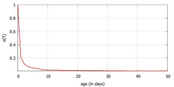
Let us define the recency property for a graph evolving in time. Denote by $e(T)$ the fraction of edges connecting nodes whose age difference is greater than $T$. We analyze the behavior of $e(T)$ and show that media pages tend to connect to pages of similar age. We plotted $e(T)$ for our dataset and noted that $e(T)$ is decreasing exponentially fast (see Figure 1), which is not the case for preferential attachment model as we show later in this paper (Section 5.2).

Figure 1: The recency property

4 Model

Suppose that we have a fixed set of hosts $H_{1},\dots,H_{n}$. Each host $H_{i}$ has its own rate of new pages appearance $\lambda_{i}$. At the beginning of the process, we have no pages. We assume that new pages appear on a host $H_{i}$ according to a Poisson process with parameter $\lambda_{i}$. A Poisson process is often used to model a sequence of random events that happen independently with a fixed rate over time. Poisson processes for different hosts are independent.

When a new page $p$ is created on a host $i$, it has $m_{p}$ mutually independent outgoing links pointing to already existing media pages. The target page of each link is determined as follows. First, the target host $k$ is chosen with probability $\rho_{ik}$ ($\sum_{k=1}^{n}\rho_{ik}=1$). Then, the probability of each page $r$ on the host $k$ to be chosen is proportional to the attractiveness of $r$, which is some function of $d_{r}$ (current incoming degree of $r$), $q_{r}$ (intrinsic quality of $r$), and $a_{r}$ (current age of $r$). Different attractiveness functions are possible:

$$f_{\tau_{k}}(d,q,a)=\left(1\text{ or }q\right)\cdot\left(1\text{ or }d\right)\cdot\left(1\text{ or }e^{-\frac{a}{\tau_{k}}}\right)\,.$$

Where $\tau_{k}$ corresponds to the mean lifetime of the decaying attractiveness for media pages on host $k$.

E.g., $f_{\tau_{k}}(d,q,a)=d$ leads to preferential attachment, while $f_{\tau_{k}}(d,q,a)=q\cdot d$ leads to fitness model. In this paper, we study different options and show which ones best depict the behavior of the Media Web.

Let us denote by $\Omega(H_{i})$ the set of pages, which belong to a host $H_{i}$. We assume that the distributions of $q_{p}$ and $m_{p}$ for $p\in\Omega(H_{i})$ are the properties of $H_{i}$. The only thing we assume about these distributions is that $q_{p}$ and $m_{p}$ have finite expectations.

5 Theoretical analysis

5.1 Incoming degree distribution

In [5, 8, 11], models without recency factor (i.e., without the factor $e^{-\frac{a}{\tau_{k}}}$ in the attractiveness function) have been analyzed. On the contrary, in this paper we show that we need the recency factor to reflect some important properties of the Media Web (see Section 5.2). Therefore we assume here that the attractiveness function has such recency factor.

Denote by $d_{p}(q_{p},t,t_{p})$ the incoming degree at time $t$ of a page $p$ created at time $t_{p}$ with intrinsic quality $q_{p}$. Let us also define, for each host $H_{k}$, the average attractiveness of its pages at time $t$:

$$W_{k}(t)=\mathbb{E}\sum_{p\in\Omega(H_{k})}f_{\tau_{k}}(d_{p}(q_{p},t,t_{p}),q_{p},t-t_{p})\,.$$ (1)

We will show in this section that $W_{k}(t)\to W_{k}$ as $t\to\infty$, where $W_{k}$ are some positive constants.

Let $M_{k}$ be the average number of outgoing links of pages $p\in\Omega(H_{k})$. Then $N_{k}=\sum_{i}\lambda_{i}M_{i}\rho_{ik}$ is the average rate of new links pointing to host $H_{k}$ appearance.

Theorem 5.1

Let $p\in\Omega(S_{k})$ be a page with quality $q_{p}$ and time of creation $t_{p}$.

• If $f_{\tau_{k}}=q\cdot d\cdot e^{-\frac{a}{\tau_{k}}}$,
  then ${d_{p}(q_{p},t,t_{p})=e^{\frac{N_{k}\tau_{k}q_{p}}{W_{k}}\left(1-e^{\frac{t_{p}-t}{\tau_{k}}}\right)}}$,
  

• If $f_{\tau_{k}}=q\cdot e^{-\frac{a}{\tau_{k}}}$,
  then $d_{p}(q_{p},t,t_{p})=\frac{N_{k}\tau_{k}q_{p}}{W_{k}}\left(1-e^{\frac{t_{p}-t}{\tau_{k}}}\right)$.

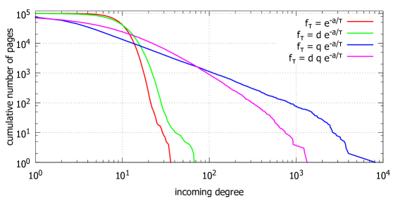
It follows from Theorem 5.1 that in the first case, in order to have a power law distribution of $d_{p}$, we need to have $q_{p}$ distributed exponentially. In this case, for each host, the parameter of the power law distribution equals $\frac{N_{k}\tau_{k}\mu}{W_{k}}$, where $\mu$ is the parameter of exponential distribution. It is interesting to note that this latter parameter cannot affect the parameter of the power law distribution. Indeed, if we multiply $\mu$ by some constant, then $W_{k}$ will also be multiplied by the same constant (see (1)). Therefore, we can change the parameter of the power law distribution only by varying $N_{k}$ and $\tau_{k}$. The problem is that the constant $W_{k}$ depends on $N_{k}$ and $\tau_{k}$ (see equation (3) in the proof). Hence, it is impossible to find analytical expressions for $N_{k}$ and $\tau_{k}$, which give us the desired parameter of the power law distribution.

In the second case, a power law distribution of $q_{p}$ leads to a power law distribution of $d_{p}$ with the same constant. Therefore, it is easy to get a realistic incoming degree distribution in this case.

In both cases, we cannot avoid the quality factor because if we do not have it in the attractiveness function (i.e., if $q_{p}$ is constant for all media pages), then the solution does not depend on $q_{p}$ and we do not have a power law for the incoming degree distribution.

To illustrate the results of Theorem 5.1, we generated graphs according to our model with different functions $f_{\tau_{k}}$. Obtained results are shown on Figure 2.

Figure 2: Incoming degree distribution for each model

Proof

In mean-field approximation, we have the following differential equation:

$$\frac{\partial d_{p}(q_{p},t,t_{p})}{\partial t}=N_{k}\frac{f_{\tau_{p}}(d_{p}(q_{p},t,t_{p}),q_{p},t-t_{p})}{W_{k}(t)},$$

here $p\in\Omega(H_{k})$.

In the case $f_{\tau_{k}}(d,q,a)=q\cdot d\cdot e^{-\frac{a}{\tau_{k}}}$ we have:

$$\frac{\partial d_{p}(q_{p},t,t_{p})}{\partial t}=N_{k}\frac{q_{p}\cdot d_{p}(q_{p},t,t_{p})\cdot e^{-\frac{t-t_{p}}{\tau_{k}}}}{W_{k}(t)}$$ (2)

Later in this section, we show that for each $k$, $W_{k}(t)$ tends to some positive constant $W_{k}$: $\lim_{t\rightarrow\infty}W_{k}(t)=W_{k}$.

We thus have the following solution of the equation (2):

$$d_{p}=e^{\frac{N_{k}\tau_{k}q_{p}}{W_{k}}\left(1-e^{\frac{t_{p}-t}{\tau_{k}}}\right)}\xrightarrow{\scriptscriptstyle t\to\infty}e^{\frac{N_{k}\tau_{k}q_{p}}{W_{k}}}$$

In case $f_{\tau_{k}}(d,q,a)=q\cdot e^{-\frac{a}{\tau_{k}}}$, by similar but even simpler calculations, we obtain:

$$d_{p}=\frac{N_{k}\tau_{k}q_{p}}{W_{k}}\left(1-e^{\frac{t_{p}-t}{\tau_{k}}}\right)\xrightarrow{\scriptscriptstyle t\to\infty}\frac{N_{k}\tau_{k}q_{p}}{W_{k}}$$

Let us now check that $\lim_{t\rightarrow\infty}W_{k}(t)$ is indeed a constant. Consider the case $f_{\tau_{k}}(d,q,a)=q\cdot d\cdot e^{-\frac{a}{\tau_{k}}}$. Let $\rho_{k}(q)$ be the probability density function of $q_{p}$ for $p\in\Omega(H_{k})$. Therefore:

$$W_{k}(t)=\int_{0}^{\infty}\left(\int_{0}^{t}\lambda_{k}q\rho_{k}(q)d(q,t,x)\cdot e^{-\frac{t-x}{\tau_{k}}}dx\right)dq=\\ =\int_{0}^{\infty}\left(\int_{0}^{t}\lambda_{k}q\rho_{k}(q)e^{\frac{N_{k}\tau_{k}q}{W_{k}}\left(1-e^{\frac{x-t}{\tau_{k}}}\right)}\cdot e^{\frac{x-t}{\tau_{k}}}dx\right)dq=\\ =\int_{0}^{\infty}\frac{\lambda_{k}W_{k}}{N_{k}}\left(e^{\frac{N_{k}\tau_{k}q}{S}\left(1-e^{\frac{-t}{\tau_{k}}}\right)}-1\right)\rho_{k}(q)dq\,.$$

Thus for $W_{k}$ we finally have the following equation:

$$W_{k}=\lim_{t\rightarrow\infty}W_{k}(t)=\underbrace{\frac{\lambda_{k}W_{k}}{N_{k}}\left(\int_{0}^{\infty}e^{\frac{N_{k}\tau_{k}q}{W_{k}}}\rho_{k}(q)dq-1\right)}_{F_{k}(W_{k})}.$$ (3)

There is a unique solution of the equation (3). To show this, we first check that ${y=F_{k}(x)}$ is monotone:

$$F_{k}^{\prime}(x)=\frac{\lambda_{k}}{N_{k}}\left(\int_{0}^{\infty}e^{\frac{N_{k}\tau_{k}q}{x}}\left(1-\frac{N_{k}\tau_{k}q}{x}\right)\rho_{k}(q)dq-1\right)\leq 0\,,$$

since:

$$e^{\frac{N_{k}\tau_{k}q}{x}}\left(1-\frac{N_{k}\tau_{k}q}{x}\right)\leq 1\text{ and }\int_{0}^{\infty}\rho_{k}(q)dq=1.$$

Also ${F_{k}(x)\to\tau_{k}\lambda_{k}\mathbb{E}_{p\in\Omega(S_{k})}q_{p}}$ as ${x\to\infty}$ and $F_{k}(x)\to\infty$ as $x\to 0$. From these observations, it follows that $y=x$ and $y=F_{k}(x)$ have a unique intersection. In other words, the equation (3) has a unique solution.

Similarly, we can show that $\lim_{t\rightarrow\infty}W_{k}(t)=W_{k}$ for the attractiveness function $f_{\tau_{k}}=q\cdot e^{-\frac{a}{\tau_{k}}}$.

5.2 Recency property

In this section, we show that we need a recency factor $e^{-\frac{a}{\tau_{k}}}$ in the formula for the attractiveness function $f_{\tau_{k}}$. We prove that because of the recency factor, the number of edges, which connect nodes with time difference greater than $T$ decreases exponentially in $T$. We prove the following theorem.

Theorem 5.2

For $f_{\tau_{k}}=q\cdot d\cdot e^{-\frac{a}{\tau_{k}}}$ or $f_{\tau_{k}}=q\cdot e^{-\frac{a}{\tau_{k}}}$ we have

$$e(T)\sim\sum_{k}N_{k}C_{k}e^{\frac{-T}{\tau_{k}}}\,,$$

where $C_{k}$ are some constants.

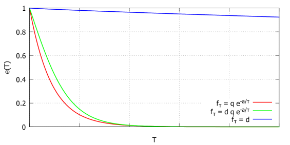
Due to space constraints, we move the proof of Theorem 5.2 to Appendix. To illustrate the results obtained, we plot $e(T)$ for different attractiveness functions on Figure 3. Note that if we have a recency factor in the attractiveness function, then $e(T)$ approaches its upper bound exponentially fast. In contrast, if the attractiveness function equals $d$ (preferential attachment), then $e(T)$ grows almost linearly with a small rate.

Figure 3: Recency property in the model

6 Validation

The idea of using Maximum Likelihood in order to compare different graph models and estimate their parameters was suggested in [4]. Since then this method was used for several models (see, e.g., [17, 18]). Motivated by these works we also use the idea of Maximum Likelihood in order to compare new models we suggest in this paper with preferential attachment and fitness models.

6.1 Parameters estimation

In order to do simulations, we first need to estimate all parameters of our models. Note that we are not trying to find the best parameters here. Instead we propose to use simple estimations, which are enough to show the improvements obtained by using our new models.

Host-to-host probabilities. We estimated the matrix $\rho_{ij}$ by counting the fraction of edges going from hosts $H_{i}$ to $H_{j}$. Note that 74% of all edges are host internal. We also add host to host probabilities to fitness and preferential attachment models and, as we show later in Section 6.2, this assumption allows to improve these models.

Estimation of $\tau$. In order to estimate $\tau_{k}$ for each host $H_{k}$, we consider the histogram of age difference of connected pages. Let $x_{i}$ ($i\geq 0$) be the number of links which connect pages with age difference greater than $i$ but less than $i+1$ days. If we assume an exponential decay, then for $i<j$ we have $\frac{x_{i}}{x_{j}}=e^{\frac{(i-j)T}{\tau_{k}}}$, i.e., $\tau_{k}=\frac{(i-j)T}{\log{\frac{x_{i}}{x_{j}}}}$, where $T$ is the time interval of one day. Therefore, we take:

$$\tau_{k}=\sum_{\begin{subarray}{c}0\leq i<j<10:\\ x_{i}\neq 0,x_{j}\neq 0\end{subarray}}\frac{(i-j)T}{{10\choose 2}\log{\frac{x_{i}}{x_{j}}}}.$$

We make a cut-off at 10 days because even though the tail of the histogram is heavier than exponential, the most important for us is to have a good estimation when pages are young, i.e. when most incoming links appear.

Estimation of quality. Given the final incoming degree $d$ of a node, we can use Theorem 5.1 to find its quality, i.e., we have $q=\frac{Wd}{N_{k}\tau_{k}}$ in the case of $f_{\tau}=qe^{\frac{-a}{T}}$ and $q=\frac{W\ln d}{N_{k}\tau_{k}}$ in the case of $f_{\tau}=dqe^{\frac{-a}{T}}$. Note that the factor $\frac{W}{N_{k}\tau_{k}}$ is common for all pages created on host $H_{k}$ and can be cancelled so we finally used the following estimations: $q=d$ and $q=\ln d$ respectively.

6.2 Likelihood

In order to valid our model, we propose to use the data described in Section 3.1 and estimate the likelihood of the real-world link graph from this data set given each model discussed in this paper. We do this as follows.

We add edges one by one according to their historical order and compute their probability given the model under consideration. The sum of logarithms of all obtained probabilities gives us the log-likelihood of our graph. We normalize this sum by the number of edges and obtained results are presented in Table 1.

Table 1: Log-likelihood table: average logarithm of edge probability.

$d$	$q$	$e^{\frac{-a}{\tau}}$	$dq$	$de^{\frac{-a}{\tau}}$	$qe^{\frac{-a}{\tau}}$	$dqe^{\frac{-a}{\tau}}$
-6.11	-5.56	-5.34	-6.08	-5.50	-5.17	-5.45

Figure 4: Distribution of edges’ probabilities

Figure 5: Distribution of edges’ probabilities relative to preferential attachment model

We see that the most likely model here is with $f_{\tau}=qe^{\frac{-a}{\tau}}$. However, since timestamps are noisy and therefore not always reliable (see Section 3.1), these results might not be representative (for example, if the probability of one edge is very small, it can heavily affect the final likelihood). Hence, in addition to this log-likelihood, which is strongly affected by outliers, we also performed the analysis of edges’ probabilities, i.e. we try to understand which model is better on a per-edge basis. We believe that such deeper analysis allows to reduce the influence of outliers when validating our models. To the best of our knowledge, this is the first time such analysis is made when using Maximum Likelihood in order to compare different graph models.

Each edge has different probabilities according to different models and there is one model $M$ for which this probability is the largest. In this case, we say that the model $M$ wins on this edge (see Table 2). Also, for each pair of models $M_{1}$ and $M_{2}$, we computed the percentage of edges which have greater probability according to $M_{1}$ than according to $M_{2}$ (see Table 3). It can be clearly seen from both tables that the recency factor plays a very important role.

Table 2: Winner table: fraction of edges on which model wins all others.

$d$	$q$	$e^{\frac{-a}{\tau}}$	$dq$	$de^{\frac{-a}{\tau}}$	$qe^{\frac{-a}{\tau}}$	$dqe^{\frac{-a}{\tau}}$
0.03	0.07	0.28	0.07	0.07	0.30	0.16

Table 3: Competition table: the value in (a,b) is the fraction of edges where $a$ wins $b$.

	$d$	$q$	$e^{\frac{-a}{\tau}}$	$dq$	$de^{\frac{-a}{\tau}}$	$qe^{\frac{-a}{\tau}}$	$dqe^{\frac{-a}{\tau}}$
$d$	-	0.22	0.30	0.43	0.18	0.22	0.19
$q$	0.78	-	0.38	0.76	0.41	0.23	0.40
$e^{\frac{-a}{\tau}}$	0.70	0.62	-	0.69	0.54	0.40	0.53
$dq$	0.57	0.24	0.31	-	0.24	0.23	0.17
$de^{\frac{-a}{\tau}}$	0.82	0.59	0.44	0.76	-	0.39	0.43
$qe^{\frac{-a}{\tau}}$	0.78	0.77	0.60	0.77	0.61	-	0.62
$dqe^{\frac{-a}{\tau}}$	0.81	0.60	0.47	0.83	0.57	0.38	-

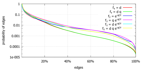
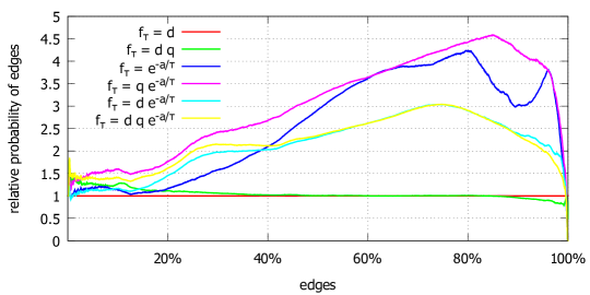
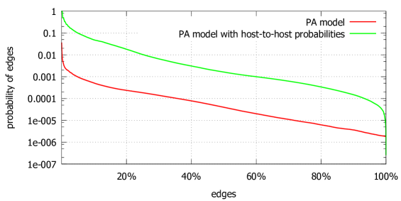
Then, for each model, we sorted edges’ probabilities in decreasing order on Figure 5. Furthermore, in order to more clearly visualize the differences between models, we normalized the probability of each edge in all models by dividing it by the corresponding probability in the sorted order of the preferential attachment model (see Figure 5). One can see that the model with $f_{\tau}=qe^{\frac{-a}{\tau}}$ again shows the best result in our tests. This means that in the Media Web the probability for a post to be cited is determined, most likely, by its quality rather than by its current popularity (i.e., incoming degree). Finally, the importance of host-to-host probabilities $\rho_{ij}$ can be illustrated by Figure 6.

Figure 6: The influence of host-to-host probabilities, e.g., on preferential attachment model (PA)

7 Conclusion

In this paper, we presented a detailed study of the Media Web. We proposed a new class of models for the appearance of new media content on the Web where different attractiveness functions of nodes are possible including ones taken from well-known preferential attachment and fitness models, but also new ones accounting for specificities of this part of the Web. Our new models are based on the observation that media pages tend to connect with other media pages of similar age.

We analyzed these models theoretically and empirically using publicly available data and show which ones realistically predict both the incoming degree distribution and the so-called recency property of the Media Web, something that existing models did not do well.

Finally we compared these models by estimating the likelihood of the real-world link graph from our data set given each model and obtained that new models we introduce, with a recency factor, are significantly more likely than previously proposed ones. One of the most surprising results is that in the Media Web the probability for a post to be cited is determined, most likely, by its quality rather than by its current popularity.

Appendix: Proof of Theorem 5.2

To analyze the behavior of $e(T)$, we need to estimate the average attractiveness of all media pages created in the last $T$ seconds at time $t$ at a host $k$:

$$\mathcal{W}_{k}(T,t)=\mathbb{E}\sum_{\begin{subarray}{c}p\in\Omega(H_{k})\\ |t-t_{p}|<T\end{subarray}}f_{\tau_{k}}(d_{p}(q_{p},t,t_{p}),q_{p},t-t_{p}).$$

We will show that if ${t>T}$, then this function does not depend on $t$.

We can analyze the function $\mathcal{W}_{k}(T,t)$ using the technique we used in Section 5.1. Consider the case $f_{\tau_{k}}(d,q,a)=q\cdot d\cdot e^{-\frac{a}{\tau_{k}}}$:

$$\mathcal{W}_{k}(T,t)=\\ =\int_{0}^{\infty}\left(\int_{t-T}^{t}\lambda_{k}q\rho_{k}(q)d(q,t,x)\cdot e^{-\frac{t-x}{\tau_{k}}}dx\right)dq=\\ =\int_{0}^{\infty}\left(\int_{t-T}^{t}\lambda_{k}q\rho_{k}(q)e^{\frac{N_{k}\tau_{k}q}{W_{k}}\left(1-e^{\frac{x-t}{\tau_{k}}}\right)}\cdot e^{\frac{x-t}{\tau_{k}}}dx\right)dq=\\ =\frac{\lambda_{k}W_{k}}{N_{k}}\int_{0}^{\infty}\left(e^{\frac{N_{k}\tau_{k}q}{W_{k}}\left(1-e^{\frac{-T}{\tau_{k}}}\right)}-1\right)\rho_{k}(q)dq\,.$$

We proved that $\mathcal{W}_{k}(T,t)$ does not depend on $t$ and will use the notation $\mathcal{W}_{k}(T)=\mathcal{W}_{k}(T,t)$ from now on. Also

$$W_{k}-\mathcal{W}_{k}(T)=\\ =\frac{\lambda_{k}W_{k}}{N_{k}}\int_{0}^{\infty}\left(1-e^{-\frac{N_{k}\tau_{k}q}{W_{k}}e^{\frac{-T}{\tau_{k}}}}\right)e^{\frac{N_{k}\tau_{k}q}{W_{k}}}\rho_{k}(q)dq\sim\\ \sim\frac{\lambda_{k}W_{k}}{N_{k}}e^{\frac{-T}{\tau_{k}}}\int_{0}^{\infty}\frac{N_{k}\tau_{k}q}{W_{k}}e^{\frac{N\tau_{k}q}{W}}\rho_{k}(q)dq\sim C_{k}e^{\frac{-T}{\tau_{k}}},$$

where the constants $C_{k}$ do not depend on $T$.

Note that the portion of links which point to the host $H_{k}$ and have the age difference less than $T$ is $\frac{W_{k}-\mathcal{W}_{k}(T)}{W_{k}}$. Thus, using $N_{k}$ which is the average rate of new links pointing to host $H_{k}$ appearance (see Section 5.1) we can write the following equation for $e(T)$:

$$e(T)=\sum_{k}N_{k}\frac{W_{k}-\mathcal{W}_{k}(T)}{W_{k}}\sim\sum_{k}\frac{N_{k}C_{k}}{W_{k}}e^{\frac{-T}{\tau_{k}}}$$

The same analysis can be made for the case $f_{\tau_{k}}(d,q,a)=q\cdot e^{-\frac{a}{\tau_{k}}}$. In this case we get:

$$\mathcal{W}_{k}(T)=\int_{0}^{\infty}\left(\int_{t-T}^{t}\lambda_{k}q\rho_{k}(q)\cdot e^{-\frac{t-x}{\tau_{k}}}dx\right)dq=\lambda_{k}\tau_{k}\left(1-e^{-\frac{T}{\tau_{k}}}\right)\mathbb{E}_{p\in\Omega(H_{k})}q_{p}\,,$$

and further reasonings are the same.

References

- [1] http://www.memetracker.org/data.html
- [2] Albert, R., Barabási, A.L.: Statistical mechanics of complex networks. Reviews of modern physics 74, 47–97 (2002)
- [3] Barabási, A.L., Albert, R.: Emergence of scaling in random network. Science 286(5439), 509–512 (1999)
- [4] Bezáková, I., Kalai, A., Santhanam, R.: Graph model selection using maximum likelihood. Proceeding ICML Proceedings of the 23rd international conference on Machine learning pp. 105–112 (2006)
- [5] Bianconi, G., Barabási, A.L.: Bose-Einstein condensation in complex networks. Physical Review Letters 86(24), 5632 –5635 (2001)
- [6] Boccaletti, S., Latora, V., Moreno, Y., Chavez, M., Hwang, D.U.: Complex networks: structure and dynamics. Physics reports 424(45), 175–308 (2006)
- [7] Bollobás, B.: Mathematical results on scale-free random graphs. Handbook of Graphs and Networks pp. 1–34 (2003)
- [8] Bollobás, B., Riordan, O., Spencer, J., Tusnády, G.: The degree sequence of a scale-free random graph process. Random Structures and Algorithms 18(3), 279–290 (2001)
- [9] Bonato, A.: A Survey of models of the web graph. Combinatorial and Algorithmic Aspects of Networking pp. 159–172 (2004)
- [10] Borgs, C., Chayes, J., Daskalakis, C., Roch, S.: First to market is not everything: an analysis of preferential attachment with fitness. Proceedings of the thirty-ninth annual ACM Symposium on Theory of Computing pp. 135–144 (2007)
- [11] Buckley, P.G., Osthus, D.: Popularity based random graph models leading to a scale-free degree sequence. Discrete Mathematics 282(1–3), 53–68 (2004)
- [12] Cooper, C., Frieze, A.: A general model of web graphs. Random Structures and Algorithms 22(3), 311–335 (2003)
- [13] Holme, P., Kim, B.: Growing scale-free networks with tunable clustering. Physical Review E 65(2) (2002)
- [14] Kumar, R., Raghavan, P., Rajagopalan, S., Sivakumar, D., Tomkins, A., Upfal, E.: Web as a graph. Proceedings of the Nineteenth ACM SIGMOD-SIGACT-SIGART Symposium on Principles of Database Systems pp. 1–10 (2000)
- [15] Lefortier, D., Ostroumova, L., Samosvat, E., Serdyukov, P.: Timely crawling of high-quality ephemeral new content. arXiv preprint arXiv:1307.6080 (2013)
- [16] Leskovec, J., Backstrom, L., Kleinberg, J.: Meme-tracking and the dynamics of the news cycle. pp. 497–506 (2009)
- [17] Leskovec, J., Backstrom, L., Kumar, R., Tomkins, A.: Microscopic evolution of social networks. Proceedings of the 14th ACM SIGKDD international conference on Knowledge Discovery and Data mining pp. 462–470 (2008)
- [18] Leskovec, J., Chakrabarti, D., Kleinberg, J., Faloutsos, C., Ghahramani, Z.: Kronecker Graphs: An Approach to Modeling Networks. The Journal of Machine Learning Research 11, 985–1042 (2010)