Validating Stochastic Models: Invariance Criteria for Systems of Stochastic Differential Equations and the Selection of a Stochastic Hodgkin-Huxley Type Model

Abstract.

In recent years, many difficulties appeared when taking into account the inherent stochastic behavior of neurons and voltage-dependent ion channels in Hodgking-Huxley type models. In particular, an open problem for a stochastic model of cerebellar granule cell excitability was to ensure that the values of the gating variables remain within the unit interval. In this paper, we provide an answer to this modeling issue and obtain a class of viable stochastic models. We select the stochastic models thanks to a general criterion for the flow invariance of rectangular subsets under systems of stochastic differential equations. We formulate explicit necessary and sufficient conditions, that are valid for both, Itô’s and Stratonovich’s interpretation of stochastic differential equations, improving a previous result obtained by A. Milian [A.Milian, Coll. Math. 1995] in the Itô case. These invariance criteria allow to validate stochastic models in many applications. To illustrate our results we present numerical simulations for a stochastic Hodgkin-Huxley model.

1. Laboratoire de Mathématiques Appliquées de Pau, Université de Pau et des Pays de l’Adour, avenue de l’Université, BP 1155, 64013 Pau Cedex, France

2. SYRTE UMR CNRS 8630, Observatoire de Paris and University Paris VI, France

3. BCAM Basque Center for Applied Mathematics, Alameda de Mazarredo 14, 48009 Bilbao, Basque Country, Spain

4. Helmholtz Zentrum München, Institut für Biomathematik und Biometrie, Ingolstädter Landstrasse 1, 85764 Neuherberg, Germany

1. Introduction

In recent years, a great deal of activities has been devoted to develop models of neuronal excitability that take into account the intrinsic stochastic bioelectrical activity of neurons (see [11], [3]). In [11], the authors apply Itô’s theory of stochastic differential equations and propose a stochastic model which reproduces the irregular electrophysiological activity of an in vitro granule cell (see [11] and Figure 6 p.7). A particular case of this model is a stochastic version of the classical Hodgkin-Huxley model (see [4], [3]). However, as already indicated by the authors, the model suffers severe difficulties ([11] p.4 and p.10): Undesired values were observed for the gating variables that are supposed to take values within the unit interval. The solution of this modeling difficulty is mentioned as a challenge for future work ([11] p.10). Similar problems also occurred for the stochastic Hodgkin-Huxley model in [3] (see p.2071). In this article, we provide an answer to this problem and obtain a family of viable stochastic models for cerebellar granule cell excitability. The admissible models are derived from a general invariance theorem for systems of stochastic differential equations.

We formulate invariance results in a general setting that allow to validate stochastic models in many applications. When the solutions of a given system of stochastic differential equations describe quantities that necessarily take values within a certain range, the problem can be mathematically analyzed by studying the flow invariance of rectangular subsets of the euclidean space. To be more precise, we consider systems of Itô differential equations of the form

$$dX(t)=f(t,X(t))dt+g(t,X(t))dW(t),$$

where the process $X$ is vector-valued. For the concrete formulation we refer to Section 2. We characterize the class of functions $f$ and $g$ that lead to viable stochastic models and formulate explicit necessary and sufficient conditions that can be directly checked and easily verified in applications. We further show that the invariance theorems are valid for both, Itô’s and Stratonovich’s interpretation of stochastic differential equations. The result for the Itô case was previously obtained by A. Milian in [7]. As discussed in [12], in a concrete application it is generally not easy to decide which interpretation should be applied. Our results show that the qualitative behavior of solutions regarding non-negativity and boundedness is independent of Itô’s or Stratonovich’s interpretation. Other properties of the solutions, however, may strongly depend on the choice of the interpretation (see [8]).

The outline of our paper is as follows: In Section 2 we introduce the class of stochastic systems we study and formulate general invariance criteria for systems of stochastic differential equations. We then apply the results to obtain viable stochastic models for cerebellar granule cell excitability in Section 3. In Section 4 we present numerical simulations to illustrate the model behaviour. Finally, in Section 5 we recall the results obtained by A. Milian in [7] and present the proofs of the invariance theorems.

2. Invariance Criteria for Stochastic Differential Equations

Let $(\Omega,\mathcal{F},P)$ be a probability space with a right-continuous increasing family $F=(\mathcal{F}_{t})_{t\geq 0}$ of sub-$\sigma$-fields of $\mathcal{F}$ each containing all sets of $P$-measure zero. We consider systems of stochastic Itô equations of the form

$$X(t)=X_{0}+\displaystyle\int_{t_{0}}^{t}f(s,X(s))ds+\int_{t_{0}}^{t}g(s,X(s))dW(s),\qquad\quad t\in[t_{0},\infty[,$$ (1)

where $f=[f_{i}]:[0,\infty[\times\mathbb{R}^{m}\rightarrow\mathbb{R}^{m}$ is Borel-measurable, and $g=[g_{ij}]:[0,\infty[\times\mathbb{R}^{m}\rightarrow\mathbb{R}^{m\times r}$ is a Borel-measurable mapping into the set of all $\mathbb{R}^{m\times r}$-matrices, $i=1,\dots,m,j=1,\dots,r$. Furthermore, $W:[0,\infty[\times\Omega\rightarrow\mathbb{R}^{r}$ denotes an $r$-dimensional $F$-Wiener process, the initial time $t_{0}$ is non-negative and $X_{0}\in\mathbb{R}^{m}$ is the given initial data.

The stochastic integral equations (1) are commonly written as system of stochastic Itô differential equations,

$$dX(t) = f(t,X(t))dt+g(t,X(t))dW(t),\qquad\quad t\in[t_{0},\infty[,$$

$$X(t_{0}) = X_{0},$$

where the function $g$ represents the stochastic perturbation and $f$ the deterministic part. Indeed, if $g\equiv 0$ we obtain the corresponding unperturbed deterministic system of ODEs.

In the sequel, we denote by $(f,g)$ stochastic initial value problems of the form (1). We aim at formulating explicit necessary and sufficient conditions on the functions $f$ and $g$ for the non-negativity and boundedness of solutions. The conditions can directly be verified and allow to explicitly characterize the class of admissible models in applications. In Section 5 we deduce our main theorems from a more general result about the stochastic invariance of polyhedral subsets of $\mathbb{R}^{m}$. However, in applications the non-negativity and boundedness of solutions are the most relevant modeling issues.

Since our aim is not to establish the well-posedness of the stochastic initial value problem but to study the qualitative behavior of solutions, we assume that for every initial time $t_{0}\geq 0$ and initial data $X_{0}\in\mathbb{R}^{m}$ there exists a unique solution of the stochastic problem (1).

Definition 1.

We say that the subset $K\subset\mathbb{R}^{m}$ is invariant for the stochastic system $(f,g)$ if for every initial data $X_{0}\in K$ and initial time $t_{0}\geq 0$ the corresponding solution $X(t)$, $t\geq t_{0}$, satisfies

$$P\left(\left\{X(t)\in K,\ t\in[t_{0},\infty[\right\}\right)=1.$$

The following theorem characterizes the class of functions $f$ and $g$ such that the stochastic system $(f,g)$ preserves the positivity of solutions. That is, solutions emanating from non-negative initial data (almost surely) remain non-negative as long as they exist.

Theorem 2.

Let $I\subset\{1,\dots,m\}$ be a non-empty subset. Then, the set

$$K^{+}:=\{x=(x_{1},\dots,x_{m})\in\mathbb{R}^{m},\ x_{i}\geq 0,\,i\in I\}$$

is invariant for the stochastic system $(f,g)$ if and only if

$$f_{i}(t,x) \geq 0\qquad\textnormal{\emph{for}}\ x\in K^{+}\ \textnormal{\emph{such that}}\ x_{i}=0,$$

$$g_{i,j}(t,x) = 0\qquad\textnormal{\emph{for}}\ x\in K^{+}\ \textnormal{\emph{such that}}\ x_{i}=0,\ j=1,\dots,r,$$

for all $t\geq 0$ and $i\in I$.

This result applies independent of Itô’s or Stratonovich’s interpretation of stochastic differential equations.

The solutions of mathematical models often describe quantities that necessarily take values within a particular range. We next formulate a criterion for the invariance of rectangular subsets of the phase space $\mathbb{R}^{m}$.

Theorem 3.

Let $I\subset\{1,\dots,m\}$ be a non-empty subset and $a_{i},b_{i}\in\mathbb{R}$ such that $b_{i}>a_{i}$. Then, the set

$$K:=\{x\in\mathbb{R}^{m}:\ a_{i}\leq x_{i}\leq b_{i},\,i\in I\}$$

is invariant for the stochastic system $(f,g)$ if and only if

$$f_{i}(t,x) \geq 0\qquad\textnormal{\emph{for}}\ x\in K\ \textnormal{\emph{such that}}\ x_{i}=a_{i},$$

$$f_{i}(t,x) \leq 0\qquad\textnormal{\emph{for}}\ x\in K\ \textnormal{\emph{such that}}\ x_{i}=b_{i},$$

$$g_{i,j}(t,x) = 0\qquad\textnormal{\emph{for}}\ x\in K\ \textnormal{\emph{such that}}\ x_{i}\in\{a_{i},b_{i}\},\ j=1,\dots,r,$$

for all $t\geq 0$ and $i\in I$.

This result is valid independent of Itô’s or Stratonovich’s interpretation.

If we apply Theorem 2 or Theorem 3 to the corresponding unperturbed deterministic system $(f,0)$ we recover the well-known tangential condition for systems of ODEs, which is necessary and sufficient for the flow invariance of subsets of $\mathbb{R}^{m}$ (see [13] or [9]).

Finally, we formulate a criterion for the validity of comparison principles for the solutions of stochastic systems. A. Milian stated the following theorem for systems of Itô equations in [7]. We recall her result and show that it remains valid if we apply Stratonovich’s interpretation of stochastic differential equations.

Theorem 4.

Let $I$ be a non-empty subset of $\{1,\dots,m\}$. We assume that $(f,g)$ and $(\tilde{f},\tilde{g})$ are stochastic systems of the form $(\ref{stochastic})$ with given initial data $X_{0},Y_{0}\in\mathbb{R}^{m}$, and denote by $X$ and $Y$ the corresponding solutions. Then, the following statements are equivalent:

• For all $t_{0}\geq 0$ and $i\in I$, if the initial data satisfy $(X_{0})_{i}\geq(Y_{0})_{i}$, then

  $$P\left(\left\{X_{i}(t)\geq Y_{i}(t),\ t\in[t_{0},\infty[,i\in I\right\}\right)=1.$$

• The functions $f,\tilde{f},g$ and $\tilde{g}$ satisfy

  $$f_{i}(t,x) \geq \tilde{f}_{i}(t,y),\ \quad\qquad t\geq 0,$$

  $$g_{ij}(t,x) = \tilde{g}_{ij}(t,y),\quad\qquad t\geq 0,\ j=1,\dots,r,$$

  for all $i\in I$ and $x,y\in\mathbb{R}^{m}$ such that $x_{i}=y_{i}$ and $x_{k}\geq y_{k}$ for $k\in I$.
  

3. The Validation of a Stochastic Hodgkin-Huxley Type Model

A stochastic model for cerebellar granule cell excitability was proposed and numerically studied in [11]. As many biophysical models of neurons it is based on the well-known deterministic Hodgkin-Huxley formalism [4], which qualitatively describes the conduction and excitation in nerves. Such models are commonly formulated as systems of deterministic ODEs. The behavior of neurons and voltage-dependent ion channels, however, is known to be stochastic in nature, which motivates the modeling approach in [11]. The mathematical model is formulated as system of stochastic differential equations for the dependent model variables $x_{i}$, which represent the gating variables for the specific ion channels, the transmembrane potential $V$ and the intracellular calcium concentration $C$,

$$dx_{i} =f_{i}(V,x_{i})dt+\sigma_{i}\,dW_{i}(t), i=1,\dots,8,$$ (2)

$$dx_{9} =f_{9}(V,C,x_{9})dt+\sigma_{9}\,dW_{9}(t),$$

$$dV =F(t,V,x_{1},\dots,x_{9})dt,$$

$$dC =G(V,C,x_{7},x_{8})dt,$$

where the reaction functions in the equations for the gating variables are given by

$$f_{i}(V,x_{i})\ =\alpha_{i}(V)(1-x_{i})-\beta_{i}(V)x_{i}, i=1,\dots,8,$$

$$f_{9}(V,C,x_{9})=\alpha_{9}(V,C)(1-x_{9})-\beta_{9}(V,C)x_{9},$$

and the rate functions for activation $\alpha_{i}$ and inactivation $\beta_{i}$ are continuous and positive. The stochastic differential equations are interpreted in the sense of Itô, $W_{i}(t),t\geq 0,$ denote standard scalar Wiener processes, $dW_{i}$ the corresponding Itô differentials, and the parameters $\sigma_{i}$ are positive and constant, $i=1,\dots,9$. For the concrete form of the interaction functions $F$ and $G$ and the complete description of the model we refer to [11].

This model extends a previous deterministic model for cerebellar granule cell excitability by adding the stochastic terms $\sigma_{i}\,dW_{i}(t)$ in the governing equations for the gating variables $x_{i}$, $i=1,\dots,9$. Ion channel stochasticity has been detected experimentally and is due to the thermal interaction of molecules constituting an ion channel. It can be observed as random opening and closing of an ion channel at an experimentally fixed membrane potential (see [11] and also [3]).

The gating variables $x_{i}$ describe the opening and closing rates of the specific ion channels and necessarily take values within the interval $[0,1]$. While the corresponding unperturbed deterministic model, where $\sigma_{i}=0,i=1,\dots,9$, certainly ensures this property, it cannot be guaranteed by the stochastic model (2):

The parameters $\sigma_{i}$, $i=1,\dots,9$, which take into account the intensity of the stochastic perturbations, were taken to be constant in the model and the simulations presented in [11]. The necessity to carefully choose these parameters was indicated. In particular, undesired values of the gating variables were observed and discussed, it was stressed that this modeling issue needed to be solved and highlighted as a challenge for future work (see [11], p.4 and p.10). Similar difficulties also occurred for the stochastic Hodgkin-Huxley model developed in [3] (see p.2071). Our results show that independent of the choice of the parameters $\sigma_{i}$ the invariance of the unit interval cannot be guaranteed by the stochastic model (2) if we take these parameters to be constant. Indeed, the conditions on the stochastic perturbations in Theorem 3 applied to the model (2) and the invariant subset

$$\widetilde{K}=\{y\in\mathbb{R}^{11},\ 0\leq y_{i}\leq 1,\,i=1,\dots,9\}$$

are never satisfied.

We obtain viable stochastic models if we replace the constants $\sigma_{i}$ by appropriate functions $g_{i}$, that ensure the desired invariance of the unit interval. To be more precise, we propose to consider models of the form

$$dx_{i} =f_{i}(V,x_{i})dt+g_{i}(t,V,C,x)\,dW_{i}(t), i=1,\dots,8,$$ (3)

$$dx_{9} =f_{9}(V,C,x_{9})dt+g_{9}(t,V,C,x)\,dW_{9}(t),$$

$$dV =F(t,V,x)dt,$$

$$dC =G(V,C,x_{7},x_{8})dt,$$

where $x=(x_{1},\dots,x_{9})$, and the stochastic perturbations $g_{i}:[0,\infty[\times\mathbb{R}^{11}\rightarrow\mathbb{R}$ satisfy

$$g_{i}(t,y)=0\qquad\quad\textnormal{for}\ y\in\widetilde{K}\ \textnormal{such that}\ y_{i}\in\{0,1\},$$

for all $t\geq 0$ and $i=1,\dots,9$.

Proposition 5.

The modified stochastic model (4) ensures that the gating variables $x_{i}$ take values within the interval $[0,1]$, for all $i=1,\dots,9$. This is valid for Itô’s and for Stratonovich’s interpretation of the stochastic differential equations.

Proof.

The statement is a direct consequence of Theorem 3 since the interaction functions $f_{i}$ and stochastic perturbations $g_{i}$ in the governing equations for the gating variables $x_{i}$, $i=1,\dots,9$, in the modified stochastic model (4) satisfy the required conditions. ∎

One possible choice for the stochastic perturbations are functions of the form

$$g_{i}(x_{i})=\sigma_{i}x_{i}(1-x_{i}),$$

with constants $\sigma_{i}\in\mathbb{R}^{+}$, $i=1,\dots,9.$

4. Numerical Simulations

To illustrate our results we present numerical simulations for a simplified version of the stochastic model discussed in the previous section and consider a stochastic version of the classical Hodgkin-Huxley model [4] Despite its simplicity, the deterministic Hodgkin-Huxley model has always been playing a very important role in the study of neuron excitability ([6]). However, stochasticity should be included in the model to take into account the stochastic behavior of the ion channel kinetics (see [6], p.558 and p.559).

(a) Gating Variables

(b) Voltage

Figure 1. Deterministic Model

The model we consider is formulated as system of ordinary differential equations for the dependent model variables $x_{i}$, $i=1,2,3$, that represent the gating variables for the specific ion channels, and the voltage $V$,

$$\frac{dx_{i}}{dt} =\alpha_{i}(V)(1-x_{i})-\beta_{i}(V)x_{i},$$ (4)

$$\frac{dV}{dt} =\frac{1}{C}[I-g_{Na}x_{1}^{3}x_{3}(V-E_{Na})-g_{K}x_{2}^{4}(V-E_{K})-g_{L}(V-E_{L})].$$

The rate functions for activation and inactivation are given by

$$\alpha_{1}(V) =\frac{0.1(V+35)}{1-\exp(-\frac{V+35}{10})}, \beta_{1}(V)=4.0\exp(-0.0556(V+60)),$$

$$\alpha_{2}(V) =\frac{0.01(V+50)}{1-\exp(-\frac{V+50}{10})}, \beta_{2}(V)=0.125\exp(-\frac{V+60}{80}),$$

$$\alpha_{3}(V) =0.07\exp(-0.05(V+60)), \beta_{3}(V)=\frac{1}{1+\exp(-0.1(V+30))},$$

and the parameter values by

$$C =0.01\frac{\mu F}{cm^{2}}, g_{Na}=1.2\frac{mS}{cm^{2}}, g_{K}=0.36\frac{mS}{cm^{2}}, g_{L}=0.03\frac{mS}{cm^{2}},$$

$$I =0.1\ mV, E_{Na}=55.17\ mV, E_{K}=-72.14\ mV, E_{L}=-49.42\ mV,$$

(see [4]).

(a) Gating Variables: $\sigma=0.1$

(b) Voltage: $\sigma=0.1$

(c) Gating Variables: $\sigma=0.5$

(d) Voltage: $\sigma=0.5$

Figure 2. Stochastic Model: Additive Noise

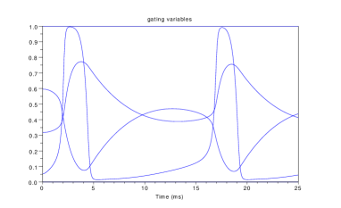
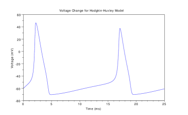
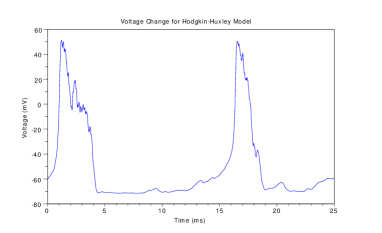
We illustrate the model behavior in Figure 1. The gating variables $x_{i}$, $i=1,2,3$, describe the opening and closing rates of the specific ion channels and necessarily take values within the interval $[0,1]$. The deterministic model (4) certainly ensures this property.

Following the modeling approach in [11], we may extend the deterministic model by adding the stochastic terms $\sigma_{i}\,dW_{i}(t)$ in the governing equations for the gating variables $x_{i}$ in the model (4), which leads to the system of stochastic differential equations

$$dx_{i}(t) =(\alpha_{i}(V(t))(1-x_{i}(t))-\beta_{i}(V(t))x_{i}(t))dt+\sigma_{i}\,dW_{i}(t),\qquad i=1,2,3.$$ (5)

We interpret the stochastic differential equations in the sense of Itô, $W_{i}(t),t\geq 0,$ denote standard scalar Wiener processes, $dW_{i}$ the corresponding Itô differentials, and the parameters $\sigma_{i}$ are positive and constant, $i=1,\dots,3$.

(a) Gating Variables: $\sigma=0.1$

(b) Voltage: $\sigma=0.1$

(c) Gating Variables: $\sigma=0.5$

(d) Voltage: $\sigma=0.5$

Figure 3. Viable Stochastic Model: Itô’s Interpretation

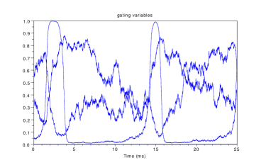
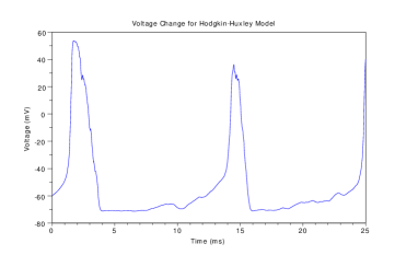
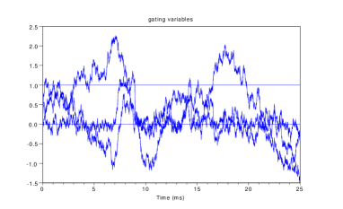
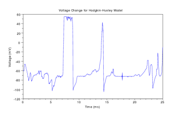
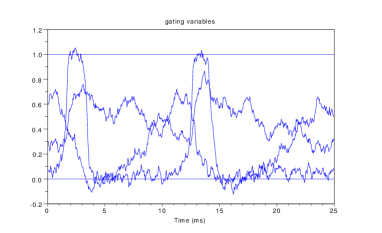
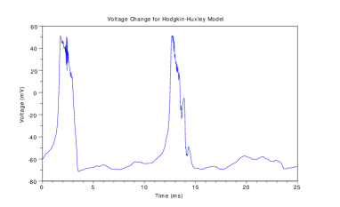
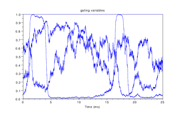
Our results in Section 2 imply that the gating variables in the model (6) take undesired values outside of the unit interval. The simulations in Figure 2 illustrate this observation for different values of the parameter $\sigma=\sigma_{i},i=1,2,3$. Here, we used the Euler-Maruyama method for the numerical implementation (see [5] and [10]). We remark that Itô’s and Stratonovich’s interpretation yield the same solution for the stochastic model (6).

(a) Gating Variables: $\sigma=0.1$

(b) Voltage: $\sigma=0.1$

(c) Gating Variables: $\sigma=0.5$

(d) Voltage: $\sigma=0.5$

Figure 4. Viable Stochastic Models: Stratonovich’s Interpretation

We obtain viable stochastic models if we replace the constants $\sigma_{i}$ in the equations for the gating variables by appropriate functions $g_{i}$, $i=1,2,3$, that ensure the desired invariance of the unit interval. To be more precise, we may consider stochastic models, where the determining equations for the gating variables $x_{i}$ are of the form

$$dx_{i}(t) =(\alpha_{i}(V(t))(1-x_{i}(t))-\beta_{i}(V(t))x_{i}(t))dt+g_{i}(t,x_{1}(t),x_{2}(t),x_{3}(t))\,dW_{i}(t),$$ (6)

for $i=1,2,3$, and the stochastic perturbations $g_{i}:[0,\infty[\times\mathbb{R}^{3}\rightarrow\mathbb{R}$ satisfy

$$g_{i}(t,x_{1},x_{2},x_{3})=0\qquad\quad\textnormal{for}\ x_{1},x_{2},x_{3}\in[0,1]\ \textnormal{such that}\ x_{i}\in\{0,1\},$$

for all $t\geq 0$ and $i=1,\dots,3$.

Theorem 3 in Section 2 immediately implies that the gating variables in the modified stochastic model (6) take values within the interval $[0,1]$, and that it is valid for Itô’s and Stratonovich’s interpretation of the stochastic differential equations.

We illustrate the model behavior for stochastic perturbations of the form

$$g_{i}(t,x_{1},x_{2},x_{3})=\sigma x_{i}(1-x_{i})\qquad\ i=1,\dots,3,$$

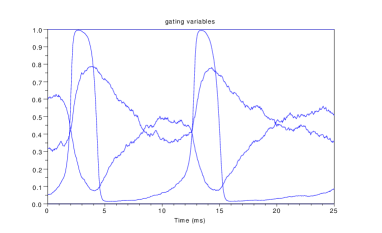
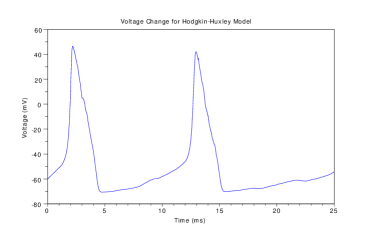
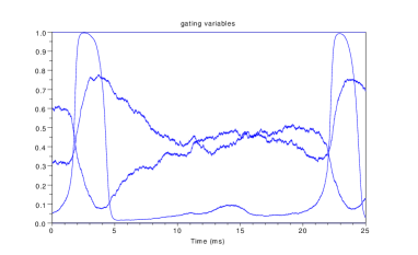
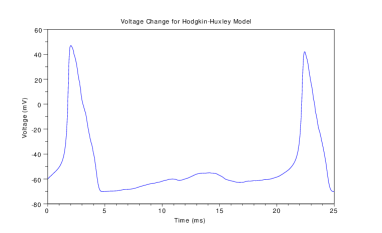
where the constant $\sigma>0$. The simulations in Figure 3 show the behavior of the solutions for Itô’s interpretation of the stochastic system (6), where we used the Euler-Maruyama method for the numerical implementation. Figure 4 illustrates the model behavior when we apply Stratonovich’s interpretation. In this case we applied the Euler-Heun method for the simulations (see [5] and [10]).

5. Proof of the Theorems

Our proof is based on the main theorems obtained by A. Milian in [7]. We first recall her results, which are formulated for systems of stochastic Itô differential equations, and yield necessary and sufficient conditions for the stochastic viability of polyhedral subsets and the validity of comparison theorems.

Definition 6.

A subset $K\subset\mathbb{R}^{m}$ is said to possess the stochastic viability property with respect to the system $(f,g)$ if for every initial data $X_{0}\in K$ and every $t_{0}\geq 0$ there exists a global solution of the initial value problem (1), and the solution satisfies

$$P\left(\left\{X(t)\in K,\ t\in[t_{0},\infty[\right\}\right).$$

For vectors $a,n\in\mathbb{R}^{m}$ we denote by

$$H_{a,n}:=\{x\in\mathbb{R}^{m},\ \langle x-a,n\rangle\geq 0\}$$

the half-space determined by $a$ and $n$, where $\langle\cdot,\cdot\rangle$ is the scalar product in $\mathbb{R}^{m}$. A polyhedron $K$ in $\mathbb{R}^{m}$ is a set of the form

$$K=\bigcap_{\nu\in I}H_{a_{\nu},n_{\nu}},$$

where $I=\{1,\dots,N\}\subset\mathbb{N}$ is a finite subset and $a_{\nu},n_{\nu}\in\mathbb{R}^{m}$, $\nu\in I$.

For the proof of the following results we refer to [7].

Theorem 7.

Let $K=\bigcap_{\nu\in I}H_{a_{\nu},n_{\nu}}$ be a polyhedron in $\mathbb{R}^{m}$ and suppose that the functions $f$ and $g$ satisfy the following conditions:

• For every $T>0$ there exists a constant $C_{T}>0$ such that

  $$\|f(t,x)\|^{2}+\|g(t,x)\|^{2}\leq C_{T}(1+\|x\|^{2})\qquad\textnormal{\emph{for all}}\ x\in K,t\in[0,T].$$

• For every $T>0$ there exists a constant $\widetilde{C}_{T}>0$ such that

  $$\|f(t,x)-f(t,y)\|+\|g(t,x)-g(t,y)\|\leq\widetilde{C}_{T}\|x-y\|\qquad\textnormal{\emph{for all}}\ x,y\in K,t\in[0,T].$$

• For every $x\in K$ the functions $f(\cdot,x)$ and $g(\cdot,x)$ are continuous on $[0,\infty[$.

Then, the set $K$ possesses the stochastic viability property with respect to the system $(f,g)$ if and only if for all $\nu\in I$ and $x\in K$ such that $\langle x-a_{\nu},n_{\nu}\rangle=0$ we have

$$\,\langle f(x,t),n_{\nu}\rangle\, \geq 0,$$

$$\langle g_{j}(x,t),n_{\nu}\rangle =0,\qquad j=1,\dots,r,$$

for all $t\geq 0$, where $g_{j}$ is the $j$-th column of the matrix $g=[g_{ij}]$.

Theorem 8.

Let $I$ be a non-empty subset of $\{1,\dots,m\}$ and suppose that for every $T>0$ there exists a constant $C_{T}>0$ such that

• $\|f(t,x)\|^{2}+\|g(t,x)\|^{2}\leq C_{T}(1+\|x\|^{2})\qquad\textnormal{\emph{for all}}\ x\in\mathbb{R}^{m},t\in[0,T].$
  

• $\|f(t,x)-f(t,y)\|+\|g(t,x)-g(t,y)\|\leq C_{T}\|x-y\|\qquad\textnormal{\emph{for all}}\ x,y\in\mathbb{R}^{m},t\in[0,T].$
  

• For every $x\in K$ the functions $f(\cdot,x)$ and $g(\cdot,x)$ are continuous on $[0,\infty[$.

We assume that the functions $\overline{f}$ and $\overline{g}$ satisfy the same conditions and denote the corresponding solutions of the stochastic systems $(f,g)$ and $(\overline{f},\overline{g})$ by $X$ and $Y$. Then, the following statements are equivalent:

• For all $t_{0}\geq 0$, $X_{0}=((X_{0})_{1},\dots,(X_{0})_{m})\in\mathbb{R}^{m}$ and $Y_{0}=((Y_{0})_{1},\dots,(Y_{0})_{m})\in\mathbb{R}^{m}$ such that $(X_{0})_{i}\geq(Y_{0})_{i},i\in I$, the corresponding solutions satisfy

  $$P(\{X_{i}(t)\geq Y_{i}(t),\ i\in I,t\geq t_{0}\})=1.$$

• For all $i\in I$ the functions $f$ and $g$ satisfy

  $$f_{i}(t,x) \geq \overline{f}_{i}(t,y)\,\qquad\textnormal{\emph{for}}\ t\geq 0,$$

  $$g_{ij}(t,x) = \overline{g}_{ij}(t,y)\qquad\textnormal{\emph{for}}\ t\geq 0,\,j=1,\dots,r,$$

  and all $x=(x_{1},\dots,x_{m})\in\mathbb{R}^{m}$, $y=(y_{1},\dots,y_{m})\in\mathbb{R}^{m}$ such that $x_{k}\geq y_{k}$, $k\in I$, $x_{i}=y_{i}$.

We remark that the assumptions (a)-(c) in Theorem 7 are imposed to guarantee the existence of solutions of the stochastic initial value problem $(f,g)$. The more restrictive hypothesis in Theorem 8 imply the existence and uniqueness of solutions, and therefore, the stochastic viability of a subset is equivalent to the stochastic invariance with respect to the system $(f,g)$.

We will deduce our criteria from Milian’s result and show that they are valid independent of Itô’s and Statonovich’s interpretation of stochastic differential equations. In the sequel, we use the symbol $\circ\,dW(t)$ to indicate Stratonovich’s interpretation. For convenience of the reader we recall the general conversion formula for systems of stochastic differential equations, which relates both interpretations (see [2], Section 6E):

If we interpret the stochastic system $(\ref{stochastic})$ in the sense of Stratonovich, that is, $X$ is the solution of the stochastic system

$$dX(t)=f(t,X(t))dt+g(t,X(t))\circ\,dW(t),$$

then, $X$ solves the system of Itô equations

$$dX(t)=\left[f(t,X(t))+\frac{1}{2}h(t,X(t))\right]dt+g(t,X(t))dW(t),$$

where the function $h=[h_{i}]:[0,\infty[\times\mathbb{R}^{m}\rightarrow\mathbb{R}^{m}$ is given by

$$h_{i}(t,x)=\sum_{k=1}^{r}\sum_{j=1}^{m}\frac{\partial g_{ik}}{\partial x_{j}}(t,x)g_{jk}(t,x),\qquad i=1,\dots,m.$$ (7)

Proof of Theorem 2.

Using polyhedral subsets of $\mathbb{R}^{m}$ the positive cone can be represented as

$$K^{+}=\bigcap_{i=1}^{m}H_{0,e_{i}},$$

where $0\in\mathbb{R}^{m}$ denotes the origin and $e_{i},i=1,\dots,m$, the standard orthonormal basis vectors in $\mathbb{R}^{m}$. Since we a priori assume the existence and uniqueness of solutions of the stochastic initial value problem $(f,g)$, the stochastic viability of the positive cone $K^{+}$ is equivalent to its invariance with respect to the system $(f,g)$. Evaluating the necessary and sufficient conditions formulated in Theorem 7 immediately follows the result for Itô’s interpretation of the stochastic system. We need to show that the statement remains valid if we apply Stratonovich’s interpretation of stochastic differential equations. Let $X$ be a solution of the Stratonovich equation

$$dX(t)=f(t,X(t))dt+g(t,X)\circ\,dW(t).$$

Then, the transformation formula implies that $X$ solves the system of Itô equations $(\hat{f},g)$ with modified interaction term $\hat{f}=f+\frac{1}{2}h$, where the function $h$ is defined by the formula (7). We apply our previous result, which is valid for Itô’s interpretation, to the stochastic system $(\hat{f},g)$ and conclude that the positive cone is an invariant subset if and only if

$$\hat{f}_{i}(t,x) \geq 0\qquad\quad x\in K^{+}\ \textnormal{such that}\ x_{i}=0,$$

$$g_{i,j}(t,x) = 0\qquad\quad x\in K^{+}\ \textnormal{such that}\ x_{i}=0,\ j=1,\dots,r,$$

for all $t\geq 0$ and $i\in I,$. The conditions on the stochastic perturbations yield the representation

$$g_{i,j}(t,x)=x_{i}\int_{0}^{1}\frac{\partial g_{i,j}}{\partial x_{i}}(t,x_{1},\dots,sx_{i},\dots,x_{m})ds\qquad\quad i\in I,=1,\dots,r,$$ (8)

and it follows that the functions $f$ and $g$ satisfy the conditions in Theorem 2 if and only if the functions $\hat{f}$ and $g$ fulfill these conditions. This observation concludes the proof for Stratonovich’s interpretation. ∎

Proof of Theorem 3.

We can represent the subset $K$ in Theorem 3 as the finite intersection of polyhedral subsets

$$K=\bigcap_{i\in I}\big{(}H_{0,e_{i}}\cap H_{e_{i},-e_{i}}\big{)}.$$

Computing explicitly the necessary and sufficient conditions for the invariance of the subset $K$ in Theorem 7 follows the statement for the system of Itô equations $(f,g)$.

To prove the result for Stratonovich’s interpretation we use the explicit relation between both interpretations and the representation (8) for the stochastic perturbations in the final part of the proof of Theorem 3. This leads to the modified system of Itô equations $(\hat{f},g)$, for which necessary and sufficient conditions are known. We observe that the conditions on the functions $f$ and $g$ are equivalent to the same conditions for the functions $\hat{f}$ and $g$, and are therefore invariant under the transformation relating both interpretations. ∎

Proof of Theorem 4.

The comparison theorem for Itô’s interpretation is valid by Theorem 8. To show the result for Stratonovich’s interpretation of stochastic differential equations we use the explicit transformation formula, which leads to the modified system of Itô equations $(\hat{f},g)$. We apply the known result for Itô’s interpretation and observe that the conditions for the functions $\hat{f}$ and $g$ are equivalent to the conditions for the functions $f$ and $g$. ∎

Concluding Remarks

We obtained necessary and sufficient conditions for the invariance of rectangular subsets of the euclidean space under systems of stochastic differential equations and proved that the invariance property is independent of Itô’s and Stratonovich’s interpretation. In particular, we were able to characterize the class of stochastic perturbations that preserve the invariance property of the unperturbed deterministic system of ODEs. Such results are very relevant for applications and allow to validate stochastic models.

When not only temporal but also spatial properties are relevant, the models are generally formulated as systems of stochastic PDEs. We are currently working on the extension of our invariance results for systems of parabolic PDEs under stochastic perturbations. A first result in this direction has been obtained in [1].

Acknowledgement: The third author is funded by the ERC Advanced Grant FPT-246775 NUMERIWAVES.

References

- [1] J. Cresson, M. Efendiev, S. Sonner, On the Positivity of Solutions of Systems of SPDEs, Zeitschrift für angewandte Mathematik und Mechanik, Journal of Applied Mathematics and Mechanics, DOI: 201100167, 2012.
- [2] L.C. Evans, An introduction to Stochastic Differential Equations: Version 1.2, Lecture Notes, UC Berkeley.
- [3] R. F. Fox, Stochastic Versions of the Hodgkin-Huxley Equations, Biophysical Journal, 72, 2068-2074, 1997.
- [4] A.L. Hodgkin, A.F. Huxley, A Quantitative Description of Membrane Current and its Application to Conduction and Excitation in Nerves, J. Physiol 117, 500-544, 1952.
- [5] P. Kloeden, E. Platen, Numerical Solution of Stochastic Differential Equations, Springer-Verlag, Berlin-Heidelberg-New York, 1999.
- [6] C. Meunier, I. Segev, Playing the Devil’s Advocate: Is the Hodgkin-Huxley Model Useful?, Trends in Neuroscience, Vol. 25, No. 11, 2002.
- [7] A. Milian, Stochastic Viability and a Comparison Theorem, Colloquium Mathematicum vol. LXVIII, Fasc. 2, 297-316, 1995.
- [8] B. Oksendal, Stochastic Differential Equations: An Introduction with Applications, 6th Edition, Springer-Verlag, Berlin-Heidelberg, 2003.
- [9] N.H. Pavel, Differential Equations, Flow Invariance and Applications, Pitman, Boston, 1984.
- [10] W. Rümelin, Numerical Treatment of Stochastic Differential Equations, SIAM Journal of Numerical Analysis 19, no. 3, 604-613, 1982.
- [11] A. Saarinen, M-L. Linne, O. Yli-Harja, Stochastic Differential Equation Model for Cerebellar Granule Cell Excitability, Plos Computational Biology, Vol. 4, Issue 2, 1-11, 2008.
- [12] M. Turelli, Random Environments and Stochastic Calculus, Theoretical Population Biology 12, 140-178, 1977.
- [13] W. Walter, Gewöhnliche Differentialgleichungen, Seventh Edition, Springer-Verlag, Berlin-Heidelberg, 2000.