Ergodicity breaking in geometric Brownian motion

Abstract

Geometric Brownian motion (GBM) is a model for systems as varied as financial instruments and populations. The statistical properties of GBM are complicated by non-ergodicity, which can lead to ensemble averages exhibiting exponential growth while any individual trajectory collapses according to its time-average. A common tactic for bringing time averages closer to ensemble averages is diversification. In this letter we study the effects of diversification using the concept of ergodicity breaking.

Geometric Brownian motion (GBM) is a useful model for systems in which the temporal evolution is strongly affected by relative fluctuations, such as stock prices and populations. Fluctuations have a net-negative effect on growth in such systems, due to the multiplicative nature of the noise. One strategy commonly employed to reduce these effects is diversification. In the language of statistical physics diversification involves a partial ensemble average (PEA) over a finite number, $N$, of trajectories generated by GBM. This raises important questions such as: How do the PEAs compare to the ensemble average ($N\to\infty$)? How and when do significant differences arise? In this letter we analyze PEAs of GBM both analytically and numerically.

In GBM it is possible for the ensemble average to grow exponentially, while any individual trajectory decays exponentially on sufficiently long time scales Peters (2011a). Multiplicative growth is manifestly non-ergodic. But precisely the opposite is often assumed in economics, for instance in Chernoff and Moses (1959), p.98: “If a gamble is ‘favorable’ from the point of view of the expectation value [ensemble average] and you have the choice of repeating it many times [time average], then it is wise to do so. For eventually, your amount of money [is] bound to increase.” Some of the consequences of this unwarranted assumption of ergodicity were pointed out in Peters (2011a), here we treat the general case of PEAs for arbitrary averaging time and sample size.

Geometric Brownian motion is defined by

$$dx=x(\mu dt+\sigma dW),$$ (1)

where $\mu$ is a drift term, $\sigma$ is a noise amplitude, and $W(t)=\int_{0}^{t}dW$ is a Wiener process. Without the noise, i.e. $\sigma=0$, the model is simply exponential growth at rate $\mu$. With $\sigma\neq 0$ it can be interpreted as exponential growth with a fluctuating growth rate.

To solve (Eq. 1), one computes the increment $d\ln(x)$ of the logarithm of $x$, integrates and exponentiates. The interesting step is computing the increment because this requires stochastic calculus. In writing (Eq. 1) we had in mind an interpretation of the equation in the Itô convention Lau and Lubensky (2007). With this convention, it is well known that $d\ln(x)=(\mu-\frac{\sigma^{2}}{2})dt+\sigma dW$, which by exponentiation implies the solution

$$x(t)=x(0)\exp\left(\left(\mu-\frac{\sigma^{2}}{2}\right)t+\sigma W(t)\right).$$ (2)

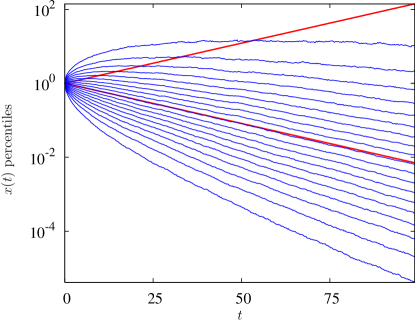
For simplicity, we will assume the initial condition $x(0)=1$. Figure  1 illustrates the nature of this process.

Figure 1: Percentiles from 95 to 5 (top to bottom) in steps of 5, based on 10,000 realizations of $x(t)$. The parameters (used for all illustrations here) are $\mu=0.05$ and $\sigma^{2}=0.2$. The red straight lines show the ensemble average (upward sloping) and an exponential decreasing with the time-average growth rate. The ensemble average is essentially meaningless for a single realization, whereas the time-average growth rate accurately describes the typical behavior.

The process $x(t)$ is not stationary. This implies that where averages can be defined, there is no guarantee for ergodicity, i.e. the equality of ensemble and time averages Gray (2009). The time average of the process itself is either 0 (if $\mu-\sigma^{2}/2<0$), or diverges positively (if $\mu-\sigma^{2}/2>0$), whereas the ensemble average is an exponential function of time. To capture the non-ergodicity of the process in well-defined averages of an observable, we define the following estimator for the exponential growth rate

$$g_{\text{est}}(t,N):=\frac{1}{t}\ln\left(\left\langle x_{i}(t)\right\rangle_{N}\right),$$ (3)

where we call $\left\langle\cdot\right\rangle_{N}:=\frac{1}{N}\sum_{i}^{N}\cdot$ a PEA. The estimator looks at the growth rate of a PEA (it is not a PEA of the growth rate), i.e. the logarithm is taken outside the average. This is crucial to leave the non-ergodic properties of the process, $x(t)$, intact. The time-average growth rate, denoted $\bar{g}$, is found by letting time remove the stochasticity in the process. Mathematically, this is the limit

$$\bar{g}:=\lim_{t\to\infty}g_{\text{est}}(t,N)=\mu-\frac{\sigma^{2}}{2}.$$ (4)

The ensemble-average growth rate, denoted $\left\langle g\right\rangle$, is found by letting an increasing ensemble size remove the stochasticity. Mathematically, this is the limit

$$\left\langle g\right\rangle:=\lim_{N\to\infty}g_{\text{est}}(t,N)=\mu.$$ (5)

The non-ergodicity of the process is manifested in the non-commutativity of the limits $\lim_{t\to\infty}$ and $\lim_{N\to\infty}$.

Both ensemble and time averages are mathematical objects and therefore separated from physical reality by the divide that separates logic from matter. Nonetheless, both averages carry practically meaningful messages. To identify the regimes where they “apply”, that is, where they reflect typical behavior, it is important to understand more about the general case where both the observation time, $t$, and the ensemble size, $N$, are finite and arbitrary.

In Peters (2011a), the time-average growth rate, (Eq. 4), was computed for a single system, $N=1$, by letting $t$ diverge. This case is related to the so-called Kelly criterion, a concept from the gambling literature Kelly Jr. (1956), discussed in Peters (2011a, b). But the case of arbitrary $N$ was not treated. The ensemble average was computed for arbitrary $t$. But the limit $N\to\infty$ was not taken explicitly, relying on the fact that in this limit the PEA, $\left\langle x_{i}(t)\right\rangle_{N}$, is the expectation value, $\left\langle x(t)\right\rangle$. Below we show that (Eq. 4) holds for arbitrary finite $N$ and characterize the process of the convergence of (Eq. 5) for arbitrary finite $t$ as $N\to\infty$.

We begin by showing that for a single instance, $N=1$, the distribution of $g_{\text{est}}(t,N=1)$ approaches a delta function centered on $\mu-\sigma^{2}/2$ in the limit $t\to\infty$.

Substituting (Eq. 2) in (Eq. 3), $g_{\text{est}}(t,N=1)=\mu-\frac{\sigma^{2}}{2}+\frac{1}{t}\sigma W(t)$. We know that the distribution of $W(t)$ is Gaussian with mean 0 and standard deviation $t^{1/2}$, which we write as $P(W(t))=\mathcal{N}(W(t);0,t^{1/2})$. To compute the distribution of $g_{\text{est}}(t,N=1)$, we use the transformation law of probabilities, $P(g)=P(W)\left|\frac{dg}{dW}\right|^{-1}$. With $dg/dW=\frac{\sigma}{t}$ and solving (Eq. 2) for $W(g)$, this yields

$$P(g_{\text{est}}(t,N=1)) =\mathcal{N}\left(g_{\text{est}};\mu-\frac{\sigma^{2}}{2},\sqrt{\frac{\sigma^{2}}{t}}\right)$$ (6)

The limiting behavior of this distribution for $t\to\infty$ is the Dirac delta function

$$\lim_{t\to\infty}P(g_{\text{est}}(t,N=1))=\delta\left(g_{\text{est}}-\left(\mu-\frac{\sigma^{2}}{2}\right)\right)$$ (7)

In other words as $t\to\infty$, the observed growth rate will differ from $\mu-\frac{\sigma^{2}}{2}$ with probability zero.

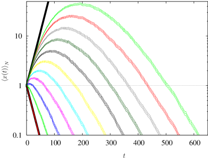
Next, we consider $N$ instances of (Eq. 1). At each moment in time, the $N$ instances are averaged, as illustrated in Fig. 2, and we are interested in the long-time behavior, $t\to\infty$, of the object $\left\langle x(t)\right\rangle_{N}$.

Figure 2: Typical trajectories $\left\langle x(t)\right\rangle_{N}$ for different ensemble sizes $N$, from top to bottom $N=1024,512...1$. For each ensemble size, 10,000 trajectories were generated. At each time the median, the 49th and 51st percentiles are shown. The solid straight red lines illustrate the ensemble-average and time-average growth rates. The single system (bottom) is dominated by time-average behavior; for increasing $N$ the trajectories stay close to the ensemble average.

Again, substituting (Eq. 2) in (Eq. 3),

$$g_{\text{est}}(t,N) =\frac{1}{t}\ln\left(\left\langle\exp\left(\left(\mu-\frac{\sigma^{2}}{2}\right)t+\sigma W_{i}(t)\right)\right\rangle_{N}\right)$$ (8)

$$=\mu-\frac{\sigma^{2}}{2}+\frac{1}{t}\ln\left(\left\langle\exp\left(\sigma W_{i}(t)\right)\right\rangle_{N}\right)$$ (9)

The difficulty with this equation is the logarithm of an average of exponentials. Unlike in the case of the single system, the logarithm does not simply undo the exponential, and the non-trivial behavior of typical trajectories of PEAs is a direct result.

To show that (Eq. 4) holds for arbitrary $N$, we will proceed in two steps by showing that as $t\to\infty$

• the probabilty of finding $g_{\text{est}}(t,N)>\mu-\frac{\sigma^{2}}{2}$ approaches zero (upper bound)

• the probabilty of finding $g_{\text{est}}(t,N)<\mu-\frac{\sigma^{2}}{2}$ approaches zero (lower bound).

Upper bound:
Equation (9) is a growth rate estimate of an average. But the average cannot be larger than the largest individual term. This establishes an inequality, namely an upper bound on $g_{\text{est}}(t,N)$.

$$g_{\text{est}}(t,N)\leq\mu-\frac{\sigma^{2}}{2}+\frac{1}{t}\sigma\max_{i}^{N}W_{i}(t).$$ (10)

A value $g_{\text{est}}(t,N)>\mu-\frac{\sigma^{2}}{2}+\epsilon$ is thus only possible if

$$\max_{i}^{N}W_{i}(t)>\frac{\epsilon t}{\sigma}.$$ (11)

The probability of such an extremum is Gumbel (1958)

$$P\left(\max_{i}^{N}W_{i}(t)>\frac{\epsilon t}{\sigma}\right)=1-\left(\int_{-\infty}^{\frac{\epsilon t}{\sigma}}\mathcal{N}(z;0,\sqrt{t})dz\right)^{N}.$$ (12)

Two interesting properties can be observed. First, for finite $N$, and $\epsilon>0$,

$$\lim_{t\to\infty}P\left(\max_{i}^{N}W_{i}(t)>\frac{\epsilon t}{\sigma}\right)=0,$$ (13)

the desired result. This is because the width of the distribution $\mathcal{N}(x;0,\sqrt{t})$ increases as $\sqrt{t}$, whereas the upper limit of the integral increases as $t$, outpacing the divergence of the width. In the limit $t\to\infty$, the entire distribution is integrated, which yields 1 due to normalization. Second, for finite $t$, the limit

$$\lim_{N\to\infty}P\left(\max_{i}^{N}W_{i}(t)>\frac{\epsilon t}{\sigma}\right)=1.$$ (14)

This must be so because the term that is being raised to the $N^{\text{th}}$ power is less than 1 for finite $t$ and therefore vanishes exponentially with $N$. In other words, in the limit of diverging ensemble size, the method fails to give an upper bound on the estimated average growth rate. This is so because $\max_{i}^{N}W_{i}(t)$ diverges in this limit.

Lower bound:
The lower bound on $g_{\text{est}}(t,N)$ is obtained in the same way as the upper bound, by switching the inequality and considering the minimum of the $N$ instances at time $t$.

We have shown that as $t\to\infty$ the probability for observing a growth rate $g_{\text{est}}(t,N)\neq\mu-\frac{\sigma^{2}}{2}$ approaches zero for any finite $N$.

In proving (Eq. 4), we have used extreme values, and they will be the key to understanding our problem: the exponential introduces a weighting that leads to a finite contribution to the average from extreme values whose relative frequencies vanish in the limit $N\to\infty$. Considering the discrete-time, discrete-space random walk, it is clear that the absolute maximum – not the typical maximum but the largest possible value – scales in a light-cone fashion as $t$ and not as $t^{1/2}$. This is reflected in two regimes of actual physical diffusion, a short-time regime where extrema among the positions of diffusing particles scale as $t$ and a long-time regime where they scale as $t^{1/2}$, beautifully illustrated in Richardson (1921) and, using the discrete multiplicative binomial process, in Redner (1990). For the Wiener process the largest possible values are infinite for any $t>0$. This is a well-known limitation of the model. As pointed out in Morse and Feshbach (1953), the canonical solution to the diffusion equation violates special relativity because it allows diffusing matter to exceed the speed of light. This is visible in the small-$t$ behavior: while for large $t$ positions at a distance $\sqrt{t}$ correspond to slow motion representing the physics well, at short times the speed of such motion diverges and becomes unphysical.

In Redner (1990) it was argued that in order to observe ensemble-average behavior ($N\to\infty$) for a time $\tau$ in a PEA, $N\sim\exp(\tau)$ multiplicative systems are required. This scaling follows from the exponential decrease with $\tau$ of the probability of $\tau$ consecutive up-moves in a random walk. The multiplicative nature of the process enhances large outliers and leads to the extreme values dominating the (linear) average behavior. After a time $\tau\sim\ln(N)$ the absolute extremes become a-typical for the ensemble size, leading to a deviation from ensemble-average behavior. The result in Redner (1990) is derived in the large $N$ limit. Here we reconsider this problem, phrasing it in terms of the stability of PEAs, and obtain a somewhat different conclusion. In particular we find that the PEA deviates from the ensemble average at an earlier time and is linearly unstable, i.e. unstable with respect to arbitrarily small perturbations coming from the noise.

We begin by defining the deviation $\epsilon_{N}(t)$ of the PEA from the ensemble average by

$$\left\langle x(t)\right\rangle_{N}=\exp(\mu t)+\epsilon_{N}(t).$$ (15)

Initially, trajectories will approximate those of the ensemble average so that we can approximate the deviation as

$$\epsilon_{N}(t)=\exp\left(\mu t+\sigma\left\langle\int_{0}^{t_{-}}dW_{i}\right\rangle_{N}\right)-\exp(\mu t).$$ (16)

Replacing $\left\langle\int_{0}^{t_{-}}dW_{i}\right\rangle_{N}$ by $\sqrt{\left\langle\left\langle W_{i}(t)\right\rangle_{N}^{2}\right\rangle}=\sqrt{\frac{t}{N}}$ we obtain an expression for the scaling behavior of the deviation

$$\epsilon_{N}(t)\sim\sigma\exp(\mu t)\sqrt{\frac{t}{N}}.$$ (17)

It can be shown that $\epsilon_{N}(t)$ is the PEA of the solution to

$$d\epsilon_{N=1}(t)=dt\mu\epsilon_{N=1}(t)+\sigma\exp(\mu t)dW$$ (18)

with the initial condition $\epsilon_{N}(t)=0$ at $t=0$. In addition equation (Eq. 17) is the lowest-order contribution in $\sigma\sqrt{\frac{t}{N}}$ from an asymptotic series generated from an iterative solution to (Eq. 1) (manuscript in preparation).

The approximation in (Eq. 16) neglects any non-linear effects. Nonetheless it is informative of the trade-off between $N$ and $t$. We can set (Eq. 17) equal to some finite value and derive an expression for the time, $\tau$, it takes to reach this deviation for a given ensemble size $N$. From (Eq. 17), this is

$$\tau\sim\frac{1}{\mu}\left(\ln\left(\epsilon_{N}(t)\sqrt{N}\right)-\ln\left(\sigma\sqrt{\tau}\right)\right)$$ (19)

Compared to the logarithmic scaling, $\tau\sim\ln(N)$, (Eq. 19) includes a correction (the second term on the right-hand side). For large characteristic times, $\tau\gg|\ln\left(\sigma\sqrt{\tau}\right)|$ (i.e. large values of $\epsilon_{N}(t)\sqrt{N})$, we can neglect this correction. Note however, that for the asymptotic expansion to be a valid approximation we must have $\sigma\sqrt{t/N}$ is small for $t=\tau$.

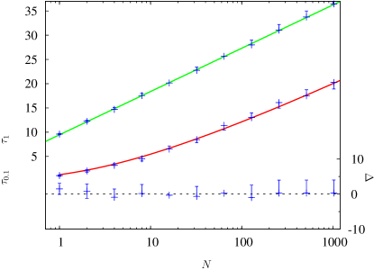
In Fig. 3 we show the times $\tau$ where absolute deviations of magnitude 0.1 and 1 of the PEA from the ensemble average were reached in the trajectories in Fig. 2.

Considering the asymptotic series from the iterative solution to (Eq. 1), we note that the amplitude of the second-order term divided by the amplitude of the first-order term for the data in Fig. 3 is less than $0.55$ for $N\geq 10$. For $\epsilon_{N}(t)=1$, where the $\ln(N)$-scaling appears to be valid, this ratio is small, namely ranging from 0.55 for $N=10$ to 0.08 for $N=1000$. It is even smaller when $\epsilon_{N}(t)=0.1$. This implies that the linear approximation is a good description for a wide range of parameters.

Figure 3: Time where the median for a given $N$, shown in Fig. 2, first differs from the ensemble average $\exp(\mu t)$ by at least 1.0 ($\tau_{1}$, top) and 0.1 ($\tau_{0.1}$, middle). Error bars show the corresponding times for the 49th and 51st percentile. A purely logarithmic fit of the form $\tau=a+b\ln(N)$ works well for deviation 1.0 (with $a=9.46$ and $b=3.88$). For deviation 0.1 occurring at smaller $t$ corrections become visible; to compare shapes the solution for $\tau(N)$ of (Eq. 19) is shown in arbitrary units. Bottom: the percentage difference, $\Delta$, between the top data and their fit.

Also features associated with much larger deviations, such as zero-crossings of the growth rate, (Eq. 3), approximately follow logarithmic scaling. This can be seen in Fig. 2, where the spacing of successive zero-crossings of the growth rate (i.e. trajectories crossing 1) is approximately constant for each doubling of $N$. For a small deviation $\epsilon_{N}(t)=0.1$ we find a non-logarithmic shape similar to (Eq. 19) including the correction.

The fact that properties of a linear approximation feed through to the full non-linear solution is surprising but not unheard-of. Equation (18) is identical to the Cahn-Hilliard-Cook theory for systems with a non-conserved order parameter which describes the evolution of a class of materials after a quench into an unstable state Gross et al. (1994). The Cahn-Hilliard-Cook theory, like (Eq. 18), is an early-time linear theory that accurately describes the sensitivity of the system to arbitrary perturbations. The implication is that early growth associated with PEAs of GBMs is inherently unstable. This leads to the conclusion that any PEA will eventually be dominated by the same time-average behavior ((Eq. 4) holds for arbitrary $N$).

In economics a mistaken belief in ergodicity has produced wide-spread conceptual inconsistency. For instance while ergodic models of exchange yield realistic predicitons for the lower part of wealth distributions, it has been pointed out that GBM-like multiplicative non-ergodic models are most natural for the upper part Yakovenko and Rosser, Jr. (2009). Under GBM, the so-called Theil index of inequality Theil (1967) can be viewed as the time-integrated difference between the time-average and ensemble-average growth rates. This difference (i.e. inequality) would be zero if GBM were ergodic. As more sophisticated and realistic economic models are studied Yakovenko and Rosser, Jr. (2009) it will be important to understand the relation between the nature of the noise, the presence of ergodicity and the properties of PEAs. Our results have important implications for the relevance of diversification strategies under realistic conditions, and the effect of multiplicative noise, in fields ranging from financial risk management to ecology, evolutionary biology, and material science.