On the shape of the mass-function of dense clumps in the Hi-GAL fields

Abstract

Context. Stars form in dense, dusty clumps of molecular clouds, but little is known about their origin and evolution. In particular, the relationship between the mass distribution of these clumps (also known as the “clump mass function”, or CMF) and the stellar initial mass function (IMF), is still poorly understood.

Aims. In order to discern the “true” shape of the CMF and to better understand how the CMF may evolve toward the IMF, large samples of bona-fide pre- and proto-stellar clumps are required. The sensitive observations of the Herschel Space Observatory (HSO) are now allowing us to look at large clump populations in various clouds with different physical conditions.

Methods. We analyse two fields in the Galactic plane mapped by HSO during its science demonstration phase, as part of the more complete and unbiased Herschel infrared GALactic Plane Survey (Hi-GAL). These fields undergo a source-extraction and flux-estimation pipeline, which allows us to obtain a sample with thousands of clumps. Starless and proto-stellar clumps are separated using both color and positional criteria to find those coincident with MIPS 24$\,\mu$m sources.

Results. We describe the probability density functions of the power-law and lognormal models that are used to fit the CMFs, and we then find their best-fit parameters. For the lognormal model we apply several statistical techniques to the data and compare their results.

Conclusions. The CMFs of the two SDP fields show very similar shapes, but very different mass scales. This similarity is confirmed by the values of the best-fit parameters of either the power-law or lognormal model. The power-law model leads to almost identical CMF slopes, whereas the lognormal model shows that the CMFs have similar widths. The similar CMF shape but different mass scale represents an evidence that the overall process of star formation in the two regions is very different. When comparing with the IMF, we find that the width of the IMF is narrower than the measured widths of the CMF in the two SDP fields. This may suggest that an additional mass selection occurs in later stages of gravitational collapse.

1 Introduction

Stars form in dense, dusty clumps of molecular clouds, but little is known about their origin and evolution (sometimes the term core is also used, see Section 3.2.1). In particular, the relationship between the mass distribution of these clumps (also known as the “clump mass function”, or CMF) and the stellar initial mass function (IMF), is poorly understood (McKee & Ostriker 2007). One of the reasons for this lack of understanding, at least from the observational point of view, has been so far the difficulty in selecting a statistically significant sample of truly pre- and proto-stellar clumps from an otherwise unremarkable collection of high column density features.

Starless (or pre-stellar, if gravitationally bound) clumps represent a very early stage of the star formation (SF) process, before collapse results in the formation of a central protostar, and the physical properties of these clumps can reveal important clues about their nature: mass, spatial distributions and lifetime are important diagnostics of the main physical processes leading to the formation of the clumps from the parent molecular cloud. In addition, a comparison of the CMF to the IMF may help to understand what processes are responsible for further fragmentation of the clumps, thus determining stellar masses. Therefore, large samples of bona-fide starless clumps are important for comparison of observations with various SF models and scenarios.

Previous studies from datasets obtained with ground facilities (e.g., Testi & Sargent 1998, Motte et al. 1998, Nutter & Ward-Thompson 2006, Enoch et al. 2008, Alves et al. 2008 and Sadavoy et al. 2010) have revealed that CMFs can roughly follow either power-law or lognormal shapes, which in some cases closely resemble the observed stellar IMF. Unfortunately, these works have also emphasized the difficulty in discerning the form of the CMF (Swift & Beaumont 2010). In fact, in some cases relatively small regions within larger clouds were examined or, even when the observations produced surveys over larger areas, they were carried out at a single wavelength (e.g., 850$\,\mu$m, 1.1 mm) and used different set of conditions to identify “clumps” in molecular clouds.

This scenario changed recently thanks to submillimeter continuum surveys based on telescopes placed on (sub)orbital platforms, namely the Balloon-borne Large Aperture Submillimeter Telescope (BLAST; Pascale et al. 2008) and the Herschel Space Observatory (HSO). BLAST carried out simultaneous observations at $\lambda=250$, 350, and 500$\,\mu$m of several Galactic star forming regions (SFRs; Chapin et al. 2008, Netterfield et al. 2009, Olmi et al. 2009, Roy et al. 2011). The even more sensitive and higher-angular resolutions observations of HSO are now allowing us to look at large clump populations in various clouds with different physical conditions, while using a self-consistent analysis to derive their physical parameters. For example, the first results from the Herschel Gould Belt Survey confirm that the shape of the pre-stellar CMF resembles the stellar IMF (André et al. 2010, Könyves et al. 2010).

In this first paper we analyse two fields in the Galactic plane mapped by HSO during its science demonstration phase (SDP). The two fields observed represent a sample of the more complete and unbiased Herschel infrared GALactic Plane Survey (Hi-GAL). Hi-GAL is a key program of HSO to carry out a 5-band photometric imaging survey at 70, 160, 250, 350, and $500\,\mu$m of a $|b|\leq 1^{\circ}$-wide strip of the Milky Way Galactic plane, originally planned for the longitude range $-60^{\circ}\leq l\leq 60^{\circ}$ (Molinari et al. 2010b), and then extended in subsequent proposals to the whole Galactic plane.

The two SDP fields have been thoroughly analyzed and have also been used to test various methods of source extraction. In addition, they have different global properties that make them interesting for the purposes of this work. Here we use these two regions as a test bed for methods of analysis that will be later applied to the rest of the Hi-GAL survey. Therefore, the conclusions of this work should be considered preliminary and specific for the SDP fields.

The outline of the paper is the following: in Section 2, we give a general description of the Hi-GAL data. In Section 3, we describe the source extraction technique and the photometry specifically adopted in this work, while we describe how the spectral energy distributions (SEDs) were assembled in Section 4. The statistical analysis of the CMFs is carried out in Sections 5 and 6. We discuss our results in Section 7 and draw our conclusions in Section 8.

2 Observations

The observations were carried out by HSO during the SDP that took place in November 2009. Five wavebands were simultaneously observed: the SPIRE instrument (Griffin et al. 2010) at $\lambda=250$, 350, and 500$\,\mu$m, and the PACS instrument (Poglitsch et al. 2010) at $\lambda=$70 and 160$\,\mu$m, were used (see Tab. 1). The two observed fields were centered at $l=30^{\circ}$ and $l=59^{\circ}$ and the final maps spanned $\simeq 2^{\circ}$ in both Galactic longitude and latitude.

The detailed description of the observation settings and scanning strategy adopted as well as the map generation procedure is given in Molinari et al. (2010a, b). Images of the SDP fields can be found in Molinari et al. (2010a) and an analysis of various general properties of these regions can be found in Battersby et al. (2011), Billot et al. (2010) and Elia et al. (2010). Here we summarize the most relevant SFRs known in both regions.

2.1 The $l=30^{\circ}$ region

The $\ell=30^{\circ}$ region that has been analyzed is approximately 4 deg² in size and is dominated by the SRBY 162 (named after Solomon et al. 1987, see also Mooney et al. 1995; also called W43-main, see Nguyen Luong et al. 2011) and SRBY 171 (also called W43-south) SFRs, with a total mass of several times $10^{6}\,M_{\odot}$. The clump of W43-main harbors a well-known giant HII region powered by a very luminous ($\sim 3.5\times 10^{6}\,L_{\odot}$, Blum et al. 1999 and references therein) cluster of Wolf-Rayet and OB stars. W43-south corresponds to a less extreme cloud, which also harbors a smaller HII region, the well-known ultra-compact HII region G29.96$-$0.02 (Cesaroni et al. 1998).

Recent analysis of the W43-main region, also in the context of the Hi-GAL project, revealed a complex structure that could be resolved into a dense cluster of protostars, infrared dark clouds, and ridges of warm dust heated by high-mass stars, thus confirming its efficiency in forming massive stars (Bally et al. 2010). While the two SDP fields seem to have similar clustering properties (Billot et al. 2011), Battersby et al. (2011) show that the median temperatures and the column densities, for all the pixels in the source masks considered, are higher in the $\ell=30^{\circ}$ field than in $\ell=59^{\circ}$. In addition, Battersby et al. (2011) also speculate that the fact that the fraction of pixels with absorption at $8\,\mu$m in the $\ell=59^{\circ}$ field is so much lower than that in the $\ell=30^{\circ}$ field, could suggest that there is a lower fraction of cold, high-column density clouds in the $\ell=59^{\circ}$ field.

Finally, the richness of the $\ell=30^{\circ}$ region in young massive stars has also been associated with it being approximately located at the interaction region between one end of the Galactic bar and the Scutum spiral arm (Garzon et al. 1997).

Table 1: PACS/SPIRE wavebands and beam FWHM. The measured beam FWHM for PACS at 70 $\mu$m is much larger than its nominal diffraction FWHM.

Instrument	Band	Beam FWHM
	[$\mu$m]	[arcsec]
PACS	70	9.2
PACS	160	12.0
SPIRE	250	17.0
SPIRE	350	24.0
SPIRE	500	35.0

2.2 The $\ell=59^{\circ}$ region

Contrary to the $\ell=30^{\circ}$ region, the $\ell=59^{\circ}$ field is not located at the tip of the Galactic bar, but belongs instead to the Sagittarius spiral arm. This region covers approximately 5 deg² and it is prominent in images of thermal dust emission as well as in the radio and the optical (see, e.g., Chapin et al. 2008 and Billot et al. 2010). The most active SFR is the Vulpecula OB association which hosts the star cluster NGC 6823 and three bright H ii regions, Sh2-86, 87 and 88. The stellar HR diagram for NGC 6823 has been examined by Massey et al. (1995). They find an age of 5–7 Myr for the bulk of the stars.

The far-infrared (60 and 100 $\mu$m) emission in this region is dominated by several luminous high-mass SFRs. Three of these have been studied by Beltrán et al. (2006) and Zhang et al. (2005) and are associated with the IRAS sources 19368+2239, 19374+2352, and 19388+2357. A further four IRAS regions (19403+2258, 19410+2336, 19411+2306, and 19413+2332) have been studied extensively by Beuther et al. (2002), using CS multi-line, multi-isotopologue observations and the 1.2 mm dust continuum.

3 Source Photometry and identification of compact sources

There is no standard terminology to identify the compact sources extracted in bolometer maps by various existing algorithms. However, while “core” usually refers to a smaller-scale object ($\mathrel{\mathchoice{\vbox{\offinterlineskip\halign{\hfil$\displaystyle#$\hfil\cr<\cr\sim\cr}}}{\vbox{\offinterlineskip\halign{\hfil$\textstyle#$\hfil\cr<\cr\sim\cr}}}{\vbox{\offinterlineskip\halign{\hfil$\scriptstyle#$\hfil\cr<\cr\sim\cr}}}{\vbox{\offinterlineskip\halign{\hfil$\scriptscriptstyle#$\hfil\cr<\cr\sim\cr}}}}0.1\,$pc), possibly corresponding to a later stage of fragmentation, the term “clump” is generally used for a somewhat larger ($\mathrel{\mathchoice{\vbox{\offinterlineskip\halign{\hfil$\displaystyle#$\hfil\cr>\cr\sim\cr}}}{\vbox{\offinterlineskip\halign{\hfil$\textstyle#$\hfil\cr>\cr\sim\cr}}}{\vbox{\offinterlineskip\halign{\hfil$\scriptstyle#$\hfil\cr>\cr\sim\cr}}}{\vbox{\offinterlineskip\halign{\hfil$\scriptscriptstyle#$\hfil\cr>\cr\sim\cr}}}}1\,$pc), unresolved object, possibly composed of several cores (Williams et al. 2000). Our maps are likely a collection of both cores and clumps; however, given the distances of the two fields being analyzed here (see Section 4 and Russeil et al. 2011), we think the term clump is more appropriate to refer to the compact objects extracted in the SDP fields. We also note that since we are constructing the clump (and not core) mass functions, with the clumps likely being composed of smaller fragments, no attempt will be made here to separate the gravitationally bound and unbound sources.

3.1 Source and flux extraction in the SPIRE/PACS maps

As we mentioned in the introduction, the SDP fields have been useful test beds for various methods of source extraction and brightness estimation. However, for the purposes of this work it was also necessary to adopt a method that in the end would be able to determine source masses, and thus the CMF, with a better accuracy compared to the original source extraction and brightness estimation pipeline described by Elia et al. (2010) and Molinari et al. (2011). This is achieved in two ways: first, the method outlined here defines in a consistent manner the region of emission of the same volume of gas/dust at different wavelengths, thus differing from the source grouping and band-merging procedures described by Molinari et al. (2011) and Elia et al. (2010). In addition, the SED fitting procedure is more accurate compared to that described by Elia et al. (2010) (see Section 4).

The source extraction and brightness estimation techniques applied to the Hi-GAL maps in this work are similar to the methods used during analysis of the BLAST05 (Chapin et al. 2008) and BLAST06 data (Netterfield et al. 2009, Olmi et al. 2009). However, important modifications have been applied to adapt the technique to the SPIRE/PACS maps, as described below.

Candidate sources are identified by finding peaks after a Mexican Hat Wavelet type convolution (MHW, hereafter; see, e.g., Barnard et al. 2004) is applied to all five SPIRE/PACS maps. Initial candidate lists from 70, 160 and $250\,\mu$m are then found and fluxes at all three bands extracted by fitting a compact Gaussian profile to the source. Sources are not identified at 350 and $500\,\mu$m due to the greater source-source and source-background confusion resulting from the lower resolution, and also because these two SPIRE wavebands are in general more distant from the peak of the source SED. The Gaussian-fitted sources are then first selected based on their integrated flux (which cannot be lower than assigned values in each waveband) and also on their FWHM, which is allowed to vary from 80% of the beam (to allow for pixelization effects on point sources) to 90 arcsec.

Each temporary source list at 70, 160 and $250\,\mu$m is then purged of overlapping sources, by comparing the positions of nearby sources at a given wavelength using their estimated FWHM: if two sources are nearer than one-half of the sum of their respective FWHMs, they are taken as being the same object. Purged lists at 70 and $160\,\mu$m are then merged, and nearby 70 and $160\,\mu$m positions are treated as before. This merged $70/160\,\mu$m catalog is then compared with the (already purged) $250\,\mu$m source list, and the same procedure is repeated for identifying overlapping objects and merge the two catalogs. Thus, a final source catalog is generated that contains well separated objects detected from all three 70, 160 and $250\,\mu$m wavebands.

In the next stage, Gaussian profiles are fitted again to all SPIRE/PACS maps, including the 350 and $500\,\mu$m wavebands, using the size and location parameters determined at the shorter wavelengths during the previous steps (the size of the Gaussian is convolved to account for the differing beam sizes). The center of the new Gaussian fit is allowed to move at most by $\simeq 5$ arcsec relative to the candidate source location, to allow for morphological differences at 350 and $500\,\mu$m, and for fitting one single Gaussian profile at those locations where more than one candidate source had been identified during the previous steps. Then, before writing the final catalog, sources are again selected using their final FWHM. Using this technique, 4702 and 2003 selected compact clumps were identified in the $\ell=59^{\circ}$ and $\ell=30^{\circ}$ fields, respectively.

Table 2: Median values of mass, temperature, distance and completeness limits toward the $\ell=30^{\circ}$ and $\ell=30^{\circ}$ fields.

Population	$\ell=30^{\circ}$ field					$\ell=59^{\circ}$ field
	Temperature	Mass	Distance	Completeness		Temperature	Mass	Distance	Completeness
	[K]	[$M_{\odot}$]	[kpc]	[$M_{\odot}$]		[K]	[$M_{\odot}$]	[kpc]	[$M_{\odot}$]
All	21.8	99.6	7.6	73.0		17.6	2.1	3.6	0.7
Starless	19.7	112.6	$-$	$-$		17.4	2.2	$-$	$-$
Proto-stellar	24.3	89.9	$-$	$-$		19.8	1.9	$-$	$-$

Monte Carlo simulations are then used to determine the completeness of this process. Following the method outlined by Netterfield et al. (2009), fake sources are added to the 160 and $250\,\mu$m maps and are then processed through the same source extraction pipeline. To generate these fake sources, we randomly select a fraction ($\sim 20-30$%) of the sources in the final catalog, we convolve them with the measured beam in each band and insert them back into the original maps. The locations of these new sources are chosen to be at least 2 arcmin from their original location, but not more than 4 arcmin, so that the fake sources will reside in a similar background environment to their original location. These added sources are not allowed to overlap each other, but are not prevented from overlapping sources originally present in the map so that the simulation will account for errors due to confusion. Therefore, the sample of fake sources approximately reproduces the distributions in intensity and size of the original catalog.

The resulting set of maps, with both original and fake sources, is run through the source extraction pipeline and the extracted source parameters are compared to the simulation input. The simulations are performed using smaller ($\simeq 0.2\,$deg²) maps, extracted from the original maps of the $\ell=59^{\circ}$ and $\ell=30^{\circ}$ fields (containing a few hundreds sources), in order to be able to run the source extraction pipeline multiple times, thus achieving a statistical average for the mass completeness limits (estimated from the $160\,\mu$m maps, at the 80% confidence level), which are listed in Table 2. These values have been estimated for the median distances of each field, also listed in the same table, and typical values of $T=20\,$K and $\beta=2$ (the dust emissivity index, see Section 4) have been used to convert the flux completeness limit into a mass completeness limit.

3.2 Separating starless and proto-stellar clumps

3.2.1 Color criteria

The catalogs of sources compiled with the technique described in §3.1 do not attempt to separate starless and proto-stellar clumps. These populations must be separated using independent methods, to ensure that they can be accurately characterized. Various criteria can be found in the literature (see, e.g., De Luca et al. 2007, Enoch et al. 2009, Netterfield et al. 2009, Olmi et al. 2009), that use both proximity criteria to infrared objects and temperature criteria. The different approaches may differ in their operational definition of the positional criteria and the identification of proto-stellar phases based on SED shape and/or other color criteria.

In this work we combine color and positional criteria. This approach has the advantage of being less computationally expensive, and least biased to particular models or model parameters, as compared to a full SED approach (e.g., Robitaille et al. 2006). Given the range of spatial resolutions and spectral coverage within the SPIRE/PACS wavebands, this combined approach should also be least biased as compared to positional criteria applied to data sets with single resolutions and limited spectral coverage.

Young protostars still embedded in dense clumps should peak in the far-infrared due to the absorption and reprocessing of light to longer wavelengths by envelopes. Several recent studies have identified these sources using IRAC and MIPS colors (e.g., Harvey et al. 2006, Jørgensen et al. 2006, 2007, 2008). Here, however, we also include the somewhat more restrictive criteria of Sadavoy et al. (2010). In fact, since embedded protostars peak in the far-infrared, we also require that proto-stellar clumps have strong detections at 24 and $70\,\mu$m and rising-red colors. The red colors will exclude stellar sources, which have flat colors in the infrared regime, but not extragalactic sources. Extragalactic contamination must be excluded separately, for example following the color criteria of Gutermuth et al. (2008). IRAC and MIPS colors were assigned to the Hi-GAL sources using the MIPSGAL catalog (Shenoy et al. 2012) and according to positional criteria (see Section 3.2.2). Our color criteria for identifying proto-stellar objects are thus as follows (see also Sadavoy et al. 2010):

• (A) The source flux at $24\,\mu$m has a signal-to-noise ratio (S/N)$\geq 3$ and the source $70\,\mu$m flux is higher than 0.1 Jy.

• (B) Source colors are dissimilar to those of star-forming galaxies (see Gutermuth et al. 2008), i.e.,

  $$\left[4.5\right]-\left[5.8\right] < \frac{1.05}{1.20}\,(\left[5.8\right]-\left[8.0\right]-1),\,\,\,{\rm and}$$

  $$\left[4.5\right]-\left[5.8\right] > 1.05,\,\,\,{\rm and}$$

  $$\left[5.8\right]-\left[8.0\right] > 1.$$

• (C1) If the source is detected at $24\,\mu$m then,

  $$\left[8.0\right]-\left[24\right] > 2.25,\,\,\,{\rm and}$$

  $$\left[3.6\right]-\left[5.8\right] > -0.28\,(\left[8.0\right]-\left[24\right])+1.88$$

• (C2) If the source is not detected at $24\,\mu$m (i.e., due to the lower sensitivity), then the IRAC bands are used,

  $$\left[3.6\right]-\left[5.8\right] > 1.25,\,\,\,{\rm and}$$

  $$\left[4.5\right]-\left[8.0\right] > 1.4.$$

It should be noted, however, that sources with no $24\,\mu$m detection, and possibly even those with no $70\,\mu$m counterpart, cannot be definitively classified as starless, at least in a low-mass clump (see Chen et al. 2010). These kind of sources may in fact represent a stage intermediate between a gravitationally-bound starless clump (i.e., pre-stellar) and a Class 0 protostar, and are difficult to identify. However, apart from these elusive objects, our color-criteria should be able to efficiently separate starless and proto-stellar clumps on a statistical basis. Separating gravitationally bound and unbound clumps is beyond the scopes of this work.

3.2.2 Positional criteria

The positional criteria to associate a MIPSGAL counterpart to the Hi-GAL sources could make the usual assumption that a given clump is to be considered proto-stellar only if a young stellar object (YSO) candidate is found in the region of a clump where the intensity of emission is higher, which is generally associated with the peak submillimeter flux. However, this simple scenario may become more complicated in confused regions, where several clumps are blended together, at which point the peak value could be off-center with respect to the volume occupied by the individual clumps.

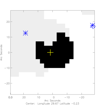
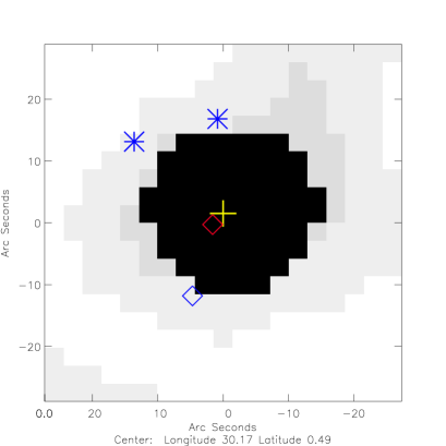
Figure 1: Top. Example of a Hi-GAL starless clump (nominal position represented with a yellow “+” sign) with an irregular shape (shown by the black area, against the gray-scale background, representing the 160 $\mu$m emission). No MIPSGAL or MHW24 source (shown with the “$\star$” and “diamond” symbols, respectively) is falling within the black area and thus they cannot be associated with the Hi-GAL source. Bottom. Example of a proto-stellar Hi-GAL clump. One MHW24 source is associated with the submillimeter clump, but no MIPSGAL source satisfies the coincidence and color criteria.

The search for YSO candidates near a given submillimeter clump is further complicated by the fact that clumps can be irregular in shape. In these cases, a circular approximation of the clump extent, by using the radius obtained with a 2-D Gaussian fit to the clump intensity distribution, could lead the search algorithm to actually probe regions beyond the “real” boundaries of the clump. On the other hand, a fixed angular tolerance could clearly lead to either underestimate or overestimate the number of YSO counterparts to the submillimeter clumps.

An alternative algorithm to ensure that the observed size and shape of the clump is considered, has been suggested by Sadavoy et al. (2010), in which the object location is compared to a percentage of the difference between the peak submillimeter intensity and the boundary intensity. Sadavoy et al. (2010) use a constant value for the boundary intensity, but in the case of the SPIRE/PACS maps, where the clump shape and intensity has to be defined with respect to the local background, we used a different approach.

First, a 1 arcmin box is extracted from the PACS $160\,\mu$m flux density map, centred around each catalog clump. To the purpose of this procedure, we think the $160\,\mu$m map constitutes the best trade-off between sensitivity and angular resolution. An average, local background level is then estimated and subtracted from the map. Intensity at the nominal position of the clump is evaluated in this background-subtracted map; the algorithm also examines the nearby pixels in case the (local) peak submillimeter intensity is off-center from the clump nominal location. The search area for coincidence with YSO candidates is then defined as all those pixels interior to the contour corresponding to a fraction $f=0.7$ of the peak intensity value found in the previous step (see Fig. 1).

The fraction $f=0.7$ has been determined by trial-and-error, and thus there were always several cases where identifying unique YSO candidates within the specified contour was not always clear, particularly in crowded regions or when a dim clump was found near a much more intense source. In these cases, the search area could result in an elongated or quite irregular shape, and we thus introduced further constraints; for example, the YSO candidate must be located within a maximum angular distance from the center of the clump, which is a function of the clump FWHM. We note that the arbitrarity of the $f=0.7$ value may lead to some cross-contamination of the starless and proto-stellar samples, but it should be statistically comparable in the two SDP fields.

The presence of a Mid-Infrared source near a Hi-GAL clump was checked in two different ways. First, the MIPSGAL catalog was used (Shenoy et al. 2012). In order to complement this catalog, we also decided to apply the source extraction algorithm described in §3.1 to the mosaicked $24\,\mu$m MIPS maps (MIPS24, hereafter) of the $\ell=59^{\circ}$ and $\ell=30^{\circ}$ fields (hereafter, we will refer to these MIPS24 sources as MHW24 objects). This approach had the advantage of being able to detect MIPS24 sources that could have been missed by the point response function fitting applied by the MIPSGAL team (Carey et al. 2009). The application of the MHW method also ensured that MIPS24 sources were extracted in a similar and uniform fashion to the SPIRE/PACS maps.

Thus, for each Hi-GAL clump, once the contour defined by $f=0.7$ was determined, the presence of both MIPSGAL and MHW24 sources within this contour was checked. If a MIPSGAL source satisfies the coincidence criterion, and if in addition its colors satisfy the criteria described in §3.2.1, then this object is assumed to be an embedded YSO and its associated Hi-GAL clump is considered to be proto-stellar. If a MHW24 source source satisfies the coincidence criterion, and if it also satisfies the color criterion (A) above, then this object is equally assumed to be an embedded YSO and its associated Hi-GAL clump proto-stellar. Thus, if either a MIPSGAL or MHW24 source satisfies the color and coincidence critaria, then the associated Hi-GAL clump is considered proto-stellar.

4 Submillimeter-MIR SEDs

As discussed by Olmi et al. (2009), our goal here is to use a simple, single-temperature SED model to fit the sparsely sampled photometry described in §3.1, which will allow us to infer the main physical parameters of each clump: mass, temperature and luminosity. These quantities must be interpreted as a parameterization of a more complex distribution of temperature and density in the clump and the equally complex response of each instrument to these physical conditions.

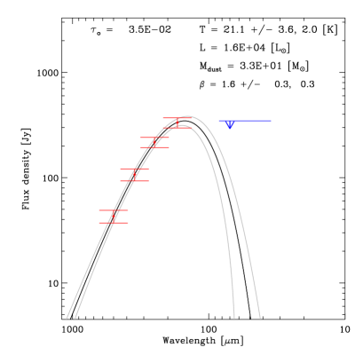
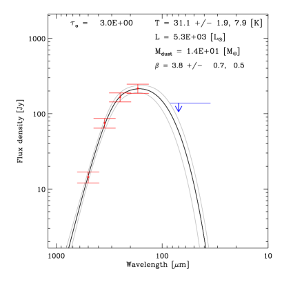
Figure 2: Top. SED of a source in the $\ell=30^{\circ}$ field. The upper limit at $70\,\mu$m is shown and black line shows the best-fit modified blackbody, whereas gray lines show the 68% confidence envelope of modified blackbody models from Monte Carlo simulations. Bottom. Another Hi-GAL clump with a more peculiar shape of the SED, due to the use of equation (1) instead of the optically-thin approximation.

In this work we mainly follow the method described by Olmi et al. (2009, and references therein). Contrary to these authors, however, we do not assume optically-thin emission and use a general isothermal modified blackbody (or gray-body) emission of the type (see, e.g., Mezger et al. 1990),

$$S_{\nu}=\Omega_{\rm s}B_{\nu}(T)\,\left[1-\exp(-\tau_{\rm d})\right],$$ (1)

where $\tau_{\rm d}$, the dust optical depth, can be written as:

$$\tau_{\rm d}=\frac{A}{\Omega_{\rm s}}\left(\frac{\nu}{\nu_{0}}\right)^{\beta}$$ (2)

where $A$ is a constant, $B_{\nu}(T)$ is the Planck function, $\beta$ is the dust emissivity index, $\Omega_{\rm s}$ is the source angular diameter (evaluated at $160\,\mu$m) and the emissivity factor is normalized at a fixed frequency $\nu_{0}$. We then write the factor $A$ in terms of a total (gas + dust) clump mass, $M$, the dust mass absorption coefficient $\kappa_{0}$ (evaluated at $\nu_{0}$), and the distance to the object, $d$:

$$A=\frac{M\kappa_{0}}{R_{\rm gd}d^{2}}.$$ (3)

The distance to individual clumps was taken from Russeil et al. (2011) when available and otherwise set to the median value (see Table 2). Since $\kappa_{0}$ refers to a dust mass, the gas-to-dust mass ratio, $R_{\rm gd}$, is required in the denominator to infer total masses. We adopt $\kappa_{0}=11$ cm² g^-1, evaluated at $\nu_{0}=c/250\,\mu$m, and $R_{\rm gd}\simeq 100$ (Martin et al. 2012).

Equation (1) is fit to all of the five SPIRE/PACS fluxes (with the PACS $70\,\mu$m flux used as upper-limit, see below), using $\chi^{2}$ optimization. Color correction of the SPIRE/PACS flux densities is performed using the filter profiles, and color-corrected fluxes are thus used in all subsequent applications. Besides to $A$ and $T$, also $\beta$ and $\Omega_{\rm s}$ are allowed to vary during the $\chi^{2}$ optimization, for a total of four free parameters.

As far as the parameter $\Omega_{\rm s}$ is concerned, this method will generally result in a different value of the source size as compared to that obtained during the source extraction procedure described in Section 3.1. This is because the source extraction procedure yields a source size mainly based on the source shape; however, the source size delivered by the $\chi^{2}$ optimization of the SED depends solely on the source photometry. In general, we find that the latter method tends to underestimate the source size obtained during the source extraction procedure.

Uncertainties for all model parameters are obtained from Monte Carlo simulations (see Chapin et al. 2008). Mock data sets are generated from realizations of Gaussian noise. The $\chi^{2}$ minimization process is repeated for each data set, and the resulting parameters are placed in histograms. Means and 68% confidence intervals are then measured from the relevant histograms. Fig. 2 shows example SEDs obtained with this procedure; the black line consists of the best-fit modified blackbody at wavelengths $>70\,\mu$m and the solid gray lines indicate the 68% confidence envelope of modified blackbodies that fit the SPIRE and PACS data.

The $70\,\mu$m flux is always treated as an upper-limit, because it would otherwise cause systematic deviations from a single-temperature gray-body fit. In fact, a non-negligible fraction of the flux at this wavelength is emitted by the warmer proto-stellar object, either formed or in advanced stage of formation at the center of the clump, while most of the emission at $\lambda\geq 160\,\mu$m originates in the colder envelope of the clump (Elia et al. 2010). We adopt “survival analysis” to properly include the upper-limit in the calculation of $\chi^{2}$ (see the discussion in Chapin et al. 2008).

5 Description of models used to fit the CMF

The goals of our analysis are to find the best fit parameters for some selected models given the data. In the following sub-sections we give a general description of the mathematical functions used in this analysis, whereas in the Appendices we outline the details of the numerical implementation, where all procedures were written in the Interactive Data Language.

5.1 Definitions

For the sake of mathematical convenience we will approximate discrete power-law and lognormal behavior with their continuous counterparts. Therefore, if ${\rm d}N$ represents the number of objects of mass $M$ lying between $M$ and $M+{\rm d}M$, the number density distribution per mass interval (or CMF), $\xi(M)={\rm d}N/{\rm d}M$, is defined through the relation (e.g., Chabrier 2003):

$$\xi(M)=\frac{{\rm d}N}{{\rm d}M}=\frac{\xi(\log M)}{M\,\ln 10}=\left(\frac{1}{M\,\ln 10}\right)\frac{{\rm d}N}{{\rm d}\log M}$$ (4)

thus, $\xi(M){\rm d}M$ represents the number of objects with mass $M$ lying in the interval $\left[M,M+{\rm d}M\right]$. The probability of a mass falling in the interval $\left[M,M+{\rm d}M\right]$ can be written for a continuous distribution as $p(M){\rm d}M$, where $p(M)$ represents the mass probability density function (PDF). The PDF and CMF must obey the following normalization conditions:

$$\int_{M_{\rm inf}}^{M_{\rm sup}}p(M){\rm d}M=1\,\,\,{\rm and}$$ (5)

$$\int_{M_{\rm inf}}^{M_{\rm sup}}\xi(M){\rm d}M=$$

$$= \int_{\log(M_{\rm inf})}^{\log(M_{\rm sup})}\xi(\log\,M){\rm d}\log\,M=N_{\rm tot}$$

where $N_{\rm tot}$ is a normalization constant which, for the case of discrete data, can be interpreted as the total number of objects being considered in the sample. From Eq. (5) $p(M)$ can also be written as $p(M)=\xi(M)/N_{\rm tot}$.

$M_{\rm inf}$ and $M_{\rm sup}$ denote respectively the inferior and superior limits of the mass range for the objects in the sample, beyond which the distribution does not follow the behavior specified by the PDF or CMF. For example, the power-law density (see Section 5.1.1) diverges as $M\rightarrow 0$ so its formal distribution cannot hold for all $M\geq 0$; there must be some lower bound to the power-law behavior, which we denote by $M_{\rm inf}$. More in general, $M_{\rm inf}$ and $M_{\rm sup}$ should give us a more quantitative estimate of the mass range where the assigned PDF gives a better description of the data.

In the following, we will also make use of the complementary cumulative distribution function (CCDF), which we denote $P_{c}(M)$ and which is defined as the probability of the mass to fall in the interval $\left[M,M_{\rm sup}\right]$, i.e.:

$$P_{c}(M)=\int_{M}^{M_{\rm sup}}p(M^{\prime}){\rm d}M^{\prime}$$ (6)

5.1.1 Powerlaw form

The most widely used functional form for the CMF is the power-law:

$$\xi_{\rm pw}(\log\,M) = A_{\rm pw}\,M^{-\alpha},\,\,\,{\rm or}$$ (7)

$$\xi_{\rm pw}(M) = \frac{A_{\rm pw}}{\ln 10}\,M^{-\alpha-1}.$$ (8)

where $A_{\rm pw}$ is the normalization constant. The original Salpeter value for the IMF is $\alpha=1.35$ (Salpeter 1955).

The PDF of a power-law (continuous) distribution is given by (e.g., Clauset et al. 2009):

$$p_{\rm pw}(M)=C_{\rm pw}\,M^{-\alpha-1}$$ (9)

where the normalization constant can be determined by applying the condition in Eq. (5), yielding:

$$C_{\rm pw}=\frac{\alpha}{(M_{\rm inf}^{-\alpha}-M_{\rm sup}^{-\alpha})}\,\,.$$ (10)

For $\alpha>0$ and $M_{\rm sup}\gg M_{\rm inf}$ one can use the approximation $C_{\rm pw}\simeq\alpha\,M_{\rm inf}^{\alpha}$ as in Clauset et al. (2009) and Swift & Beaumont (2010) (when the proper adjustments for the different definition of the power-law exponent in Eq. (8) are done).

According to Elmegreen (1985) power-laws tend to arise when only the fragments can fragment, and lognormals arise when both the fragments and the interfragment gas can fragment during a hierarchical process of star formation. However, the power-law functional form is also widely used because of its versatility. Past surveys of SFRs (see for example Swift & Beaumont 2010 and references therein) have shown a variety of values for $\alpha$, and the same dataset can be typically fit by one or more power-laws with different slopes. In particular, the power-law behavior does not extend to very low masses, where it displays a turnover or break below typically a few $M_{\odot}$.

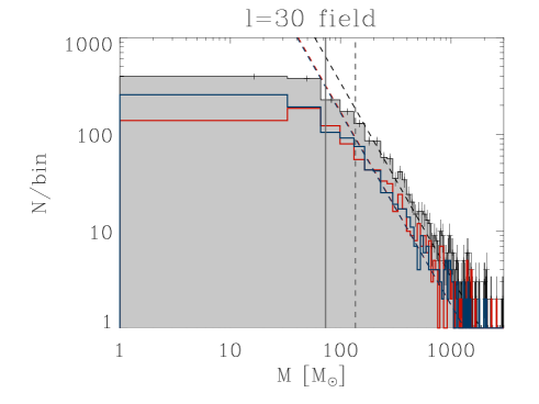
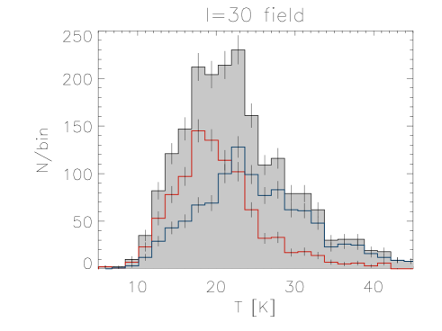
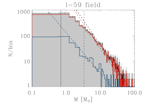
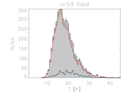
Figure 3: Left panels. Log-log histograms showing the distribution of $M$ for all (black), starless (red) and proto-stellar (blue) clumps in the $\ell=30^{\circ}$ (top) and $\ell=59^{\circ}$ (bottom) fields. The bin width has been chosen according to the Freedman and Diaconis’ rule (see Section 6.3). The dashed lines represent the results of fit to the data using the procedure PLFIT. The vertical dashed line corresponds to the value of $M_{\rm inf}$, whereas the solid vertical line shows the 80% completeness limits (see Section 3.1 and Table 2). Vertical bars show Poisson errors. Right panels. Histograms showing the distribution of clump temperature (color codes are as in the left panels) in the $\ell=30^{\circ}$ (top) and $\ell=59^{\circ}$ (bottom) fields. The bin width has also been chosen according to the Freedman and Diaconis’ rule. Line styles are as before.

Table 3: Best-fit parameters (from PLFIT) to the CMF of the $\ell=30^{\circ}$ and $\ell=59^{\circ}$ fields, for the power-law distribution. The Salpeter value of the power-law exponent for the IMF is $\alpha=1.35$ (Salpeter 1955).

Population	$\ell=30^{\circ}$ field			$\ell=59^{\circ}$ field
	$\alpha$	$M_{\rm inf}$		$\alpha$	$M_{\rm inf}$
		[$M_{\odot}$]			[$M_{\odot}$]
All	$1.15\pm 0.15$	$212\pm 79$		$1.20\pm 0.15$	$7.3\pm 2.2$
Starless	$1.12\pm 0.18$	$206\pm 95$		$1.23\pm 0.17$	$7.5\pm 2.3$
Proto-stellar	$1.06\pm 0.21$	$138\pm 105$		$0.58\pm 0.22$	$0.7\pm 2.5$

5.1.2 Lognormal form

Another widely used functional form for the CMF is the lognormal, which can be rigorously justified because the central limit theorem applied to isothermal turbulence naturally produces a lognormal PDF in density. A CMF consistent with a lognormal form has also been observed in recent surveys of nearby SFRs (see, e.g., Enoch 2006). The continuous lognormal CMF can be written (e.g., Chabrier 2003):

$$\xi_{\rm ln}(\ln\,M)=\frac{A_{\rm ln}}{\sqrt{2\pi}\,\sigma}\,\exp\left[-\frac{(\ln M-\mu)^{2}}{2\sigma^{2}}\right]$$ (11)

where $\mu$ and $\sigma^{2}=\langle(\ln M-\langle\ln M\rangle)^{2}\rangle$ denote respectively the mean mass and the variance in units of $\ln M$. $A_{\rm ln}$ represents a normalization constant which is evaluated in Appendix A.

The PDF of a continuous lognormal distribution can be written as (e.g., Clauset et al. 2009):

$$p_{\rm ln}(M) = \frac{C_{\rm ln}}{M}\,\exp\left[-\frac{(\ln M-\mu)^{2}}{2\sigma^{2}}\right]=$$

$$= \frac{C_{\rm ln}}{M}\,\exp\left[-x^{2}\right]$$

Again, by applying the normalization condition, Eq. (5), we find:

$$C_{\rm ln}=\sqrt{\frac{2}{\pi\sigma^{2}}}\,\times\left[{\rm erfc}(x_{\rm inf})-{\rm erfc}(x_{\rm sup})\right]^{-1}$$ (13)

where the variables $x$, $x_{\rm inf}$ and $x_{\rm sup}$ are defined in Appendix A, and we note that the parameters $M_{\rm inf}$ and $M_{\rm sup}$ are not necessarily the same as those determined for the power-law distribution. As we already mentioned in Section 5.1.1, if the condition $M_{\rm sup}\gg M_{\rm inf}$ holds, then we can write:

$$C_{\rm ln}\simeq\sqrt{\frac{2}{\pi\sigma^{2}}}\,\times\left[{\rm erfc}(x_{\rm inf})\right]^{-1}$$ (14)

Then, by using the definition of PDF given in Section 5.1 and the relations for the erf and erfc functions shown in Appendix A, the CCDF for the lognormal distribution, $P_{c}^{\rm ln}(M)$, can be written as:

$$P_{c}^{\rm ln}(M)=\left[\frac{{\rm erfc}(x)-{\rm erfc}(x_{\rm sup})}{{\rm erfc}(x_{\rm inf})-{\rm erfc}(x_{\rm sup})}\right]$$ (15)

6 Fitting the data

6.1 Evaluating the global CMF

In this section we apply several statistical methods to analyze the CMF of the two regions, and find the best-fit parameters for power-law and lognormal models. An important question is whether the source sample for which the CMF is constructed should undergo more specific selection criteria, such as distance, cloud or cluster location, etc. The two SDP fields may be divided into smaller sub-regions, each containing clumps in various stages of evolution as well as already formed stars. Each sub-region is in turn characterized by locally different mass distributions, which may be functions of the radial distance from the region’s center (see, e.g., Dib et al. 2010). The mass function of clumps in an entire SDP field is thus the sum of all the sub-regions and “local” distributions.

The analysis of the effects of all these local distributions on the CMF of a larger (several sq. degrees) region is out of the scopes of this work. We do not attempt to separate the complete source sample of a given SDP region into somewhat smaller sub-samples. Here we limit ourselves to address the differences, if any, between the global CMF of the two regions and postpone the study of the aforementioned effects to future work. Thus, while each source has been assigned a specific distance, when evaluating the distance effects between the two SDP fields we only consider the median distance of each region (see Section 7.3.1). Clearly, this also means that the CMF will be affected by distance-dependent sensitivity and completeness effects. However, this approach will allow us to determine if there are any significant differences with previous surveys, where the source sample is usually smaller and confined to a single cloud.

6.2 Fitting the power-law form with the method of maximum likelihood

Various methods exist to fit a parametric model to an astronomical dataset (see, e.g., Babu & Feigelson 2006). One of the most popular methods to analyze the mass spectra of the starless and proto-stellar clump populations, consists of placing the masses of individual clumps in logarithmically spaced bins, with a lower limit on the error estimated from the Poisson uncertainty for each bin. The resulting CMF can then be fitted with either a power-law or a lognormal function. Then, the resulting best-fit slope, $\alpha$, and the parameters of the lognormal function, $\mu$ and $\sigma$, usually depend somewhat on the histogram binning, and the selected mass range, particularly when “small” samples of sources are used.

Alternatively, we have considered a method described by Babu & Feigelson (2006) and more in details by Clauset et al. (2009), that consists of a statistically principled set of techniques that allow for the validation and quantification of power-laws. According to Clauset et al. (2009), this method should be quite immune to the significant systematic errors that may affect the histogram technique, including those uncertainties associated with the histogram binning. Clauset et al. (2009) have described a procedure that implements both the discrete and continuous maximum likelihood estimator (MLE) for fitting the power-law distribution to data, along with a goodness-of-fit based approach to estimating the lower cutoff of the data. Hereafter, we will refer to this procedure simply as “PLFIT”, from the name of the main MATLAB function performing the aforementioned statistical operations. The results of the PLFIT method are shown in Fig. 3 and Table 3, and are discussed in Section 7.

6.3 Fitting the lognormal form

Like Section 6.2, also in the case of the lognormal distribution we want to avoid the uncertainties inherent in fitting data using regression models arising from data binning. The first method we describe here is thus based on Bayesian regression techniques. In particular we have used WinBUGS, a programming language based software that is used to generate a random sample (using Markov chain Monte Carlo, or MCMC, methods) from the posterior distribution of the parameters of a Bayesian model. As it is customary in Bayesian regression techniques (e.g., Gregory 2005), once the posterior distributions of the parameters of interest have been generated, they can be analyzed using various descriptive measures. In Table 4 we show the mean values obtained for the $\mu$ and $\sigma$ parameters from 10000 samples MCMC runs in WinBUGS. We note that the procedure implemented in WinBUGS does not currently allow to estimate the $M_{\rm inf}$ and $M_{\rm sup}$ parameters. In the left panels of Fig. 4 we also show the histograms of the $\ln(M)$ values, with the solid lines representing Guassian fits to the histograms obtained with a standard regression technique. Both histograms and fits are shown for graphical purposes only.

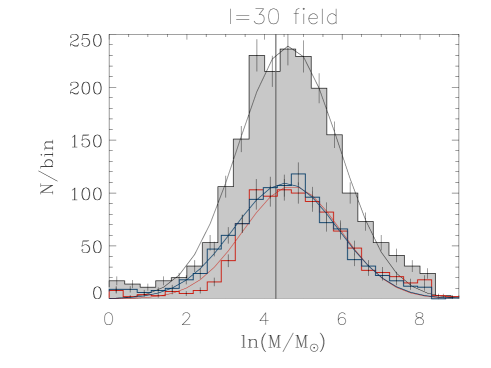
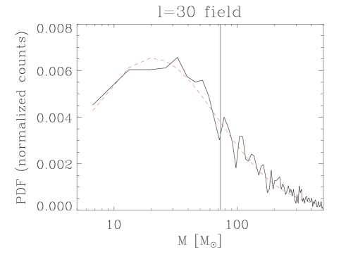
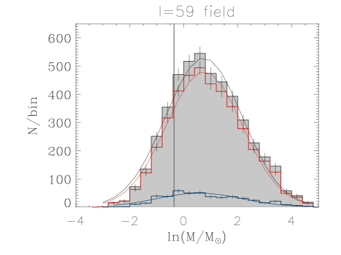
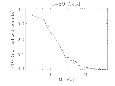
Figure 4: Left panels. Histograms showing the distribution of $\ln(M)$ for all (black), starless (red) and proto-stellar (blue) clumps in the $\ell=30^{\circ}$ (top) and $\ell=59^{\circ}$ (bottom) fields. The solid lines represent the results of Gaussian fits to the histograms. The vertical solid lines represent the completeness limits as in Fig. 3. Vertical bars show Poisson errors. Right panels. PDFs of the mass distribution (black solid line) and best-fit (red dashed line), in the $\ell=30^{\circ}$ (top) and $\ell=59^{\circ}$ (bottom) fields.

Table 4: Mean values, obtained using WinBUGS, from the posterior distributions of the $\mu$ and $\sigma$ parameters of the lognormal distribution, shown separately for the $\ell=30^{\circ}$ and $\ell=59^{\circ}$ fields.

Population	$\ell=30^{\circ}$ field			$\ell=59^{\circ}$ field
	$\mu$	$\sigma$		$\mu$	$\sigma$
	[$\ln M_{\odot}$]	[$\ln M_{\odot}$]		[$\ln M_{\odot}$]	[$\ln M_{\odot}$]
All	$4.58\pm 0.03$	$1.57\pm 0.03$		$0.91\pm 0.02$	$1.43\pm 0.02$
Starless	$4.76\pm 0.05$	$1.50\pm 0.03$		$0.92\pm 0.02$	$1.42\pm 0.02$
Proto-stellar	$4.41\pm 0.05$	$1.62\pm 0.04$		$0.89\pm 0.07$	$1.54\pm 0.04$

While we consider the results from the Bayesian regression technique our baseline results, we also want to compare them with two alternative methods. The first one is based on the computation of the PDF of the mass distribution, and is actually dependent on data binning. To compute the PDF, we plot in the right panels of Fig. 4 the normalized counts, i.e., the count per bin divided by the product of the total number of data points in the sample, $N$, and the (linear) bin width. For this normalization, the area under the histogram is equal to one, as described in Section 5.1. From a probabilistic point of view, this normalization results in a relative histogram that is most akin to the PDF. In addition, the bin width, $W$, has been chosen according to the Freedman and Diaconis’ rule (Freedman & Diaconis 1981) $W=2(IQR)N^{-1/3}$, where $IQR$ represents the inter-quartile range. The best-fit results to the PDF from standard regression techniques are then listed in Table 5.

The final method we describe here to fit the CMF with a lognormal distribution, consists of implementing a MLE method for the lognormal function, similar to the one described in Section 6.2 for the power-law distribution. The main advantage of the MLE technique, compared to the other methods, is to allow the computation of the $M_{\rm inf}$ and $M_{\rm sup}$ parameters. Therefore, we have numerically maximized the likelihood of the distribution in Eq. (5.1.2) as a function of $\sigma$ and $\mu$, using Powell’s method (e.g., Press et al. 2002). The results of this method are also listed in Table 5 ($4^{\rm th}$ and $5^{\rm th}$ column). In this first instance of the MLE method for the lognormal distribution, however, the values of $M_{\rm inf}$ and $M_{\rm sup}$ were arbitrarily fixed to constant values.

Table 5: Best-fit parameters to the CMF of the $\ell=30^{\circ}$ and $\ell=59^{\circ}$ fields, for the lognormal distribution and the PDF and MLE methods. The PDF best-fits are shown in the right panels of Fig. 4.

Region		PDF best-fit			MLE			MLE with KS
		$\mu$	$\sigma$		$\mu$	$\sigma$		$\mu$	$\sigma$	$M_{\rm inf}$	$M_{\rm sup}$
		[$\ln M_{\odot}$]	[$\ln M_{\odot}$]		[$\ln M_{\odot}$]	[$\ln M_{\odot}$]		[$\ln M_{\odot}$]	[$\ln M_{\odot}$]	[$M_{\odot}$]	[$M_{\odot}$]
$\ell=30^{\circ}$		4.5	1.2		4.5	2.3		4.7	2.9	20	394
$\ell=59^{\circ}$		0.54	1.2		1.1	2.6		0.53	1.9	0.5	10.8

Alternatively, we may consider the values of $M_{\rm inf}$ and $M_{\rm sup}$ to be also unknown. These parameters can then be found by minimizing the Kolmogorov-Smirnov (KS) statistic between the best fit model and the data as a function of $M_{\rm inf}$ and $M_{\rm sup}$ (see Appendix B). These latter results are listed in the columns $6-9$ of Table 5.

7 Discussion

7.1 $\ell=30^{\circ}$ field

As shown in Section 6.2, because of our large sample of sources, we were able to apply the PLFIT procedure not only to the whole sample of clumps detected toward the $\ell=30^{\circ}$ field, but also to the starless and proto-stellar clump samples, separately. Irrespectively of the specific sample used, we obtained $\alpha\simeq 1.1$ (see Fig. 3 and Table 3). For $M_{\rm inf}$, which represents the break or turnover below which the distribution does not follow power-law behavior, we find $M_{\rm inf}\sim 200\,M_{\odot}$, except for the sample of proto-stellar clumps where $M_{\rm inf}=138\,M_{\odot}$ but it has a large uncertainty.

In comparing our results with previous surveys we prefer to use the results of Swift & Beaumont (2010), who applied similar statistical techniques to various (smaller) datasets from the literature. In particular, for the power-law functional form, we prefer not to compare our best-fit parameters with corresponding parameters obtained using regression models depending on data binning, which are subject to large uncertainties, especially when the sample is relatively small (a few hundred sources or less).

Thus, in terms of the power-law functional form, the estimated value of $\alpha$ agrees very well with the typical values found by Swift & Beaumont (2010), for both low- and high-mass SFRs. On the other hand, the estimated value of $M_{\rm inf}\sim 200\,M_{\odot}$, is higher compared to the values estimated by Swift & Beaumont (2010) for intermediate- and high-mass SFRs. We also note the similar values of $\alpha$ and (to a lesser extent) $M_{\rm inf}$ for the starless and proto-stellar clump samples.

As far as the lognormal fits are concerned, Table 4 shows that the starless population in $\ell=30^{\circ}$ has a slightly higher (lower) value of $\mu$ ($\sigma$) compared to the proto-stellar population. More Hi-GAL fields need to be observed to determine whether this is a general property. In terms of the other statistical methods, in Table 5 we note that while the results of the MLE and PDF methods yield $\mu$ values quite similar to the Bayesian results, the values of $\sigma$ can differ significantly (by almost a factor of 2). We also note the relatively small value of $M_{\rm sup}$, compared to the whole range of masses in the $\ell=30^{\circ}$ field.

It is worth noting that the completeness limit of the $\ell=30^{\circ}$ field (see Table 2) is lower than the $M_{\rm inf}$ value. Therefore, the peak of the $\ln(M)$ distribution in Fig. 4 is real, though barely constrained. Likewise, the turnover or break in the CMF of Fig. 3 is also effectively observed. However, the fact that the turnover is not better constrained may render all later comparisons between the power-law and lognormal distributions problematic.

7.2 $\ell=59^{\circ}$ field

As shown in Table 3 (see also Fig. 3) we find that the values of $\alpha$ in the $\ell=59^{\circ}$ field are also approximately equal for the whole sample and the starless clumps. These values are consistent, within the errors, with those found in the $\ell=30^{\circ}$ field, as discussed in Section 7.3.1. However, the $\alpha$ value for the proto-stellar clumps is indeed lower than that for the starless sample. Given the much smaller number of proto-stellar clumps in the $\ell=59^{\circ}$ field, we need to further investigate whether this could be a consequence of statistical uncertainty, or it is instead a true property of this region.

Interestingly, the value of $M_{\rm inf}$ estimated in the $\ell=59^{\circ}$ region is much lower than that of the $\ell=30^{\circ}$ field, as expected given that the $\ell=59^{\circ}$ field is mostly a low- to intermediate-mass SFR. However, contrary to the $\ell=30^{\circ}$ region, our estimated value of $M_{\rm inf}$ is comparable to the values estimated by Swift & Beaumont (2010) for low-mass SFRs. On the other hand, while Swift & Beaumont (2010) report a wide range of CMF slopes (corresponding to $\alpha\sim 0.7-3.1$), our estimated values of $\alpha$ do not appreciably vary from the $\ell=30^{\circ}$ to the $\ell=59^{\circ}$ field.

In terms of the lognormal functional form of the CMF toward the $\ell=59^{\circ}$ field, the results shown in Fig. 4 and Tables 4 and 5 confirm that the mass range in the two SDP fields are quite different (see Table 2). As in the $\ell=30^{\circ}$ region, Table 5 shows that the values of $\sigma$ obtained through the MLE and PDF methods can significantly differ from the Bayesian results. We have yet to determine if this is a feature associated with the different methods.

Finally, the completeness limit of the $\ell=59^{\circ}$ region is quite lower than its corresponding $M_{\rm inf}$ value. Therefore, the peak of the $\ln(M)$ distribution in Fig. 4 is at least partially resolved, and the detection of a turnover in the CMF is more reliable than it is in the $\ell=30^{\circ}$ field.

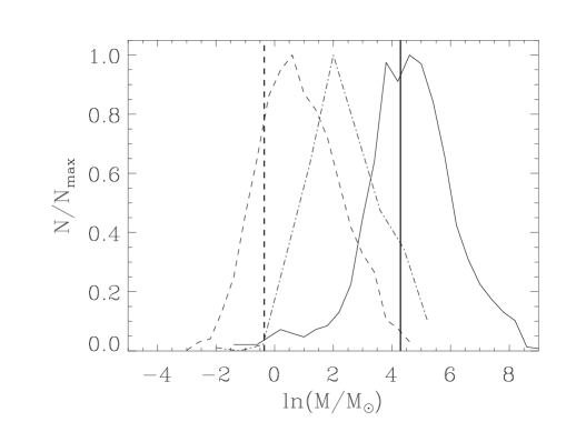
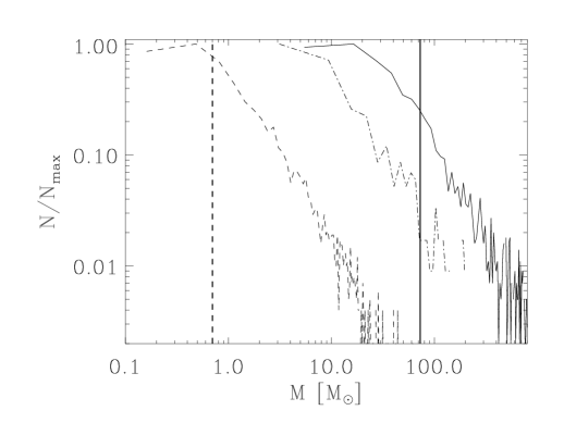
Figure 5: Top. Histogram profiles from Fig. 4, with solid and dashed lines representing the $\ell=30^{\circ}$ and $\ell=59^{\circ}$ fields, respectively. The dash-dotted line represents the distribution obtained for the $\ell=59^{\circ}$ field traslated to the distance of $\ell=30^{\circ}$ (see text). Bottom. CMF profiles from Fig. 3; line styles are as before. The vertical lines mark the completeness limits listed in Table 2 for the $\ell=30^{\circ}$ (solid line) and $\ell=59^{\circ}$ (dashed line) fields.

7.3 Comparing the two SDP fields

7.3.1 Distance effects

Comparing now the results for the $\ell=30^{\circ}$ and $\ell=59^{\circ}$ fields, we have already noted how the values of $\alpha$ are similar for the two regions. Therefore, if the evolution toward the IMF of high-mass clumps ($\ell=30^{\circ}$) is different from those of low- and intermediate-mass clumps ($\ell=59^{\circ}$), it leaves no trace on the shape of the CMF of these two regions. This conclusion, however, is critically dependent on the correcteness of the distance estimates, and in any case it is the result of a survey over a large collection of different SFRs. In fact, our findings in the $\ell=30^{\circ}$ field are different from those of Netterfield et al. (2009) who found a different slope of the CMF for the cold and warm populations of clumps in the Vela-C region, which is a less heterogeneous region compared to our field.

We have also seen that the values of $\mu$ and $M_{\rm inf}$ are clearly different for the two regions (see Tables 4 and 5). However, and despite the uncertainty on the absolute value of $\sigma$, when comparing the results obtained with the same regression technique in the two SDP fields, we find that the values of $\sigma$ are remarkably similar. We can also estimate the average values from all four methods used, and we find $\langle\sigma\rangle=2.0\pm 0.8$ and $1.8\pm 0.6$ $[\ln\,M_{\odot}]$ for $\ell=30^{\circ}$ and $\ell=59^{\circ}$, respectively. These average values are also consistent with the range of $\sigma$ found by Swift & Beaumont (2010), $\sim 0.7\,{\rm to}\,3.4$, who also found the variation in the values of $\mu$ ($\sim-5.4\,{\rm to}\,2.7$) larger compared to that of $\sigma$. Therefore, the histograms representing the distribution of the $\ln(M)$ values in the two SDP fields (Fig. 4) are characterized by decidedly different mass scales, but are quite similar in shape, as it can be noted in the left panels of Fig. 4.

This similarity can be noted even more clearly in the top panel of Fig. 5, where the histogram profiles from Fig. 4, for the $\ell=30^{\circ}$ and $\ell=59^{\circ}$ fields, are shown side by side. We also compare the CMFs in the bottom panel of Fig. 5. Apart from differences due to binning, one can clearly see that the mass distributions are very similar, although this similarity should be taken as far as the completeness limits actually allow to.

Thus, although a full comparison of the mass spectra, including the mass range below the peak of the $\ln(M)$ distribution, will require higher sensitivities than those achieved in the two SDP fields, the existence of a mass scale difference between the two regions is clear. It seems unlikely that the different mass scales could be due entirely to differences in the median distance (see Tab. 2), since this could account for a factor $\sim 4$ at most in mass sensitivity.

To test this issue more quantitatively, we have performed a simulation where the $\ell=59^{\circ}$ field is traslated to the same distance as the $\ell=30^{\circ}$ region. In this procedure, the angular resolution in all of the original maps is first degraded by convolving with a beam in each band enlarged for the increased distance, and then the maps are re-binned accordingly (A. Facchini, priv. comm.). The resulting maps are run through the source extraction and SED-fitting pipelines, and the extracted SED parameters are estimated by scaling the distance of each source by the ratio of the median distances in the $\ell=30^{\circ}$ and $\ell=59^{\circ}$ fields.

Our test thus shows that the mass of the sources in the traslated maps can increase due to the larger distance and, to a lesser extent, due to the “merging” of sources that are detected as separate objects in the original maps of the $\ell=59^{\circ}$ region. The new mass distribution is shown in Fig. 5, where we can clearly see that the CMF for the traslated $\ell=59^{\circ}$ region lies between the original CMFs of the $\ell=59^{\circ}$ and $\ell=30^{\circ}$ fields. This appears to confirm our earlier assumption that distance effects alone cannot explain the overall difference in mass scales between these two specific SFRs. We thus think that this mass scale effect is evidence that the overall process of star formation in the two regions must be radically different.

7.3.2 Clump formation efficiency

It is too early to speculate about the physical origins of the differences described in the previous section. In fact, we have exploited only a few percent of the Hi-GAL survey in the present analysis. With more and more regions being analyzed we expect to find statistically significant indications that there may indeed exist different Galactic star-forming regimes, as stated in the Hi-GAL scientific goals. For the present analysis, the prominence of the $\ell=30^{\circ}$ region in star-forming indicators, compared to $\ell=59^{\circ}$ (Battersby et al. 2011), including the (triggered) W43 “mini-starburst” complex (Bally et al. 2010), and the mass scale difference we found between the two regions, could all be related with the $\ell=30^{\circ}$ field being located near the interaction region between one end of the Galactic bar and the Scutum spiral arm, where high concentrations of shocked gas are more likely to be found (Garzon et al. 1997, López-Corredoira et al. 1999).

In order to further test this scenario, we have estimated an additional figure of merit, the clump formation efficiency ($CFE$), that we define as:

$$CFE=\frac{M_{\rm clumps}}{M_{\rm clumps}+M_{\rm clouds}}$$ (16)

where $M_{\rm clumps}$ represents the total mass of the clumps (above completeness limit) and $M_{\rm clouds}$ is the mass of the ambient gas. Given that the two SDP fields represent a collection of regions, possibly at different distances, rather than being a single molecular cloud at a single distance, two obvious problems must be considered. First off, we have to select a method to map the total column density, without being limited by threshold, opacity and temperature variations in the ambient gas/dust. Second, the distance to separate parcels of gas must be estimated.

Goodman et al. (2009) have discussed and compared several methods for measuring column density in molecular clouds and they conclude that dust extinction is likely the best probe. Therefore, we have downloaded the $A_{\rm v}$ extinction maps obtained by Rowles & Froebrich (2009) and Froebrich & Rowles (2010) and used them to estimate the total column density in the two SDP regions. Specifically, we have selected only those pixels with $A_{\rm v}>1$ and we have assigned them a distance based on the closest (within a 3 arcmin radius) mass clump previously identified. Then, the extinction in each pixel has been converted to column density using the conversion factor $N_{\rm H}=\beta_{\rm v}\,A_{\rm v}\,$cm^-2 where $\beta_{\rm v}=2\times 10^{21}\,$cm${}^{-2}\,$mag^-1 (Savage & Mathis 1979). Therefore, the total mass in the clouds has been calculated as:

$$M_{\rm clouds}=\Delta\Omega\,\mu\,\beta_{\rm v}\,m_{\rm H2}\sum_{i}d_{\rm i}^{2}A_{\rm v}^{\rm i}$$ (17)

where $\Delta\Omega$ is the solid angle subtended by each pixel in the extinction maps, $\mu=1.38$ takes into account the cosmic He abundance, $m_{\rm H2}$ is the mass of molecular hydrogen, and $d_{\rm i}$ and $A_{\rm v}^{\rm i}$ represent the distance and visual extinction toward the $i-$th pixel.

Our estimated $CFE$ thus amounts to $\simeq 2.4\,$% and $\simeq 0.7\,$% for the $l=30^{\circ}$ and $l=59^{\circ}$ regions, respectively. Although the determination of the $CFE$ is subject to several uncertainties (mainly due to the distance estimates), this is an indication that clumps may indeed form more efficiently in the $l=30^{\circ}$ rather than in the $l=59^{\circ}$ field. However, since the relationship of the $CFE$ with the star formation efficiency ($SFE$) is not known, our present analysis is not yet conclusive that the $SFE$ is also higher in the $l=30^{\circ}$ field.

7.4 Comparing the CMF to the IMF

The qualitative similarity, observed in past studies, between the CMF and the IMF offers support for the accepted idea that stars form from dense clumps, and thus comparing the two distributions should allow us to learn how observed samples of clumps evolve into stars. This comparison is actually a complex task because CMFs are often different but the IMF appears to be quite universal. In addition, it is difficult to understand whether the CMFs of different regions are intrinsically different, or to what degree systematic differences in each dataset (either observational or from post-processing) may contribute to the variations seen from dataset to dataset.

Swift & Williams (2008) have shown that different evolutionary pathways from clumps to stars produce variations in the form of the resultant IMF. They also showed that while the power-law slope is quite robust, the width of the lognormal distribution is a more sensitive indicator of clump evolution. As we showed earlier, the average value of $\sigma$ in the two SDP fields is $\sim 1.9$ $[\ln\,M_{\odot}]$, consistent with the range of $\sigma$ found by Swift & Beaumont (2010), and with an uncertainty of as much as 40%. However, the width of the IMF has been measured to be narrower, between 0.3 and 0.7 $[\ln\,M_{\odot}]$ (e.g., Chabrier 2003). As already suggested by Swift & Beaumont (2010) this would appear to indicate that an additional mass selection occurs in later stages of gravitational collapse.

8 Conclusions

We have analysed two fields mapped by the SPIRE and PACS instruments of HSO during its science demonstration phase. The two fields, which are part of the Herschel infrared GALactic Plane Survey, were centered at $l=30^{\circ}$ and $l=59^{\circ}$ and the final maps covered almost 10 deg² of galactic plane.

The two regions underwent a source-extraction and flux-estimation pipeline, which allowed us to obtain a sample with thousands of clumps. We then applied several statistical methods to analyze the resulting CMFs, and found the best-fit parameters for power-law and lognormal models. No attempt was made to select more uniform sub-samples, except for starless and proto-stellar clumps. Our main conclusions are the following:

• Our best-fit parameters for the power-law distribution show a robust slope ($\alpha\simeq 1.2$, with a $\sim\,15$% uncertainty) when comparing the two SDP fields. In contrast, we find a very different value of the parameter $M_{inf}$ for the two regions analyzed. We find that $M_{\rm inf}$ is higher than the completeness limit in each region and is thus well defined.
  

• We have used several statistical techniques to estimate the best-fit parameters of the lognormal functional form. For each separate method, the values of the width, $\sigma$, in the two SDP fields are remarkably similar. The average values, $\langle\sigma\rangle=1.9\pm 0.8$ and $1.8\pm 0.6$ $[\ln\,M_{\odot}]$ for $\ell=30^{\circ}$ and $\ell=59^{\circ}$, respectively, are also very similar. Like $M_{\rm inf}$, the value of the characteristic mass, $\mu$, is very different in the two regions.
  

• The similarity of $\alpha$ and $\sigma$ on one side, and the difference of $M_{\rm inf}$ and $\mu$ on the other, show that the CMFs of the two SDP fields have very similar shapes but different mass scales which, according to our simulations, cannot be explained by distance effects alone. This represents an evidence that the overall process of star formation in the two regions is very different.
  

• The similarity of the shape of the CMF in the two SDP regions suggests that if the evolution toward the IMF of high-mass clumps ($\ell=30^{\circ}$) is different from those of low- and intermediate-mass clumps ($\ell=59^{\circ}$), it leaves no trace on the shape of the CMF.
  

• The width of the IMF is narrower than the measured values of $\sigma$ in the two SDP fields. This suggests that an additional mass selection occurs in later stages of gravitational collapse.
  

Appendix A Normalization of the lognormal Mass Function

By applying the normalization condition (5) to the lognormal MF in Eq. (11), we get:

$$\int_{\ln(M_{\rm inf})}^{\ln(M_{\rm sup})}\frac{A_{ln}}{\sqrt{2\pi}\sigma}\,\exp\left[-\frac{(\ln M-\mu)^{2}}{2\sigma^{2}}\right]{\rm d}\ln\,M =$$

$$= N_{\rm tot}$$

which by changing the variable of integration can be easily transformed into:

$$\frac{A_{ln}}{\sqrt{\pi}}\,\int_{x_{\rm inf}}^{x_{\rm sup}}\exp(-x^{2}){\rm d}x=N_{\rm tot}$$ (18)

where we have defined the variable $x(M)=(\ln M-\mu)/(\sqrt{2}\sigma)$, and $x_{\rm inf}=x(M_{\rm inf})$ and $x_{\rm sup}=x(M_{\rm sup})$. Then, by using the following relation

$$\int_{0}^{x_{1}}\exp(-x^{2}){\rm d}x+\int_{x_{1}}^{x_{2}}\exp(-x^{2}){\rm d}x +$$

$$+\int_{x_{2}}^{\infty}\exp(-x^{2}){\rm d}x=\int_{0}^{\infty}\exp(-x^{2}){\rm d}x = \frac{\sqrt{\pi}}{2}$$

which converts into:

$$\int_{x_{1}}^{x_{2}}\exp(-x^{2}){\rm d}x = \frac{\sqrt{\pi}}{2}\left[1-{\rm erf}(x_{1})-{\rm erfc}(x_{2})\right]=$$

$$= \frac{\sqrt{\pi}}{2}\left[{\rm erfc}(x_{1})-{\rm erfc}(x_{2})\right]$$

we can write Eq. (18) as:

$$\frac{A_{ln}}{2}\,\left[1-{\rm erf}(x_{\rm inf})-{\rm erfc}(x_{\rm sup})\right]=N_{\rm tot}$$ (20)

where the ${\rm erf}$ and ${\rm erfc}$ are defined as:

$${\rm erf}(x)=\frac{2}{\sqrt{\pi}}\int_{0}^{x}\exp(-t^{2}){\rm d}t\,\,\,{\rm and}$$

$${\rm erfc}(x)=1-{\rm erf}(x)=\frac{2}{\sqrt{\pi}}\int_{x}^{\infty}\exp(-t^{2}){\rm d}t\,.$$

Finally, we can write the normalization constant, $A_{ln}$, as:

$$A_{ln}=2N_{\rm tot}\times$$ (21)

$$\left[{\rm erfc}\left(\frac{(\ln M_{\rm inf}-\mu)^{2}}{2\sigma^{2}}\right)-{\rm erfc}\left(\frac{(\ln M_{\rm sup}-\mu)^{2}}{2\sigma^{2}}\right)\right]^{-1}.$$

Appendix B Estimating the $M_{\rm inf}$ and $M_{\rm sup}$ parameters

The most common and easiest ways of choosing the $M_{\rm inf}$ and $M_{\rm sup}$ parameters (for both the power-law and lognormal functional forms) are either to take the minimum (above the completeness limit) and maximum values of the mass range in the dataset, or to plot a histogram of $M$ and choose ${M}_{\rm inf}$ and ${M}_{\rm sup}$ based on a (arbitrary) threshold occupancy for the bins. A more robust approach is desirable. In the method we use here, we choose the values of ${M}_{\rm inf}$ and ${M}_{\rm sup}$ that make the probability distributions of the observed data and the best-fit lognormal model as similar as possible in the range $\left[{M}_{\rm inf},{M}_{\rm sup}\right]$ (Clauset et al. 2009).

There are a variety of measures for quantifying the distance between two probability distributions, and following Clauset et al. (2009) we choose the Kolmogorov-Smirnov (or KS) statistics, which is simply the maximum distance between the CCDFs (see Section 5.1) of the observed data, $P_{c}^{\rm obs}(M)$, and the fitted model, $P_{c}^{\rm mod}(M)$:

$$D={\rm max}_{{}_{\left[M_{\rm inf}\leq M\leq M_{\rm sup}\right]}}|P_{c}^{\rm obs}(M)-P_{c}^{\rm mod}(M)|$$ (22)

The procedure that implements this method thus follows four basic steps:

• (1) choose $M_{\rm inf}$ and $M_{\rm sup}$ from selected (arbitrary) intervals;

• (2) calculate the MLE values of $\mu$ and $\sigma$ using Powell’s method;

• (3) apply the KS statistic to the interval $\left[{M}_{\rm inf},{M}_{\rm sup}\right]$ and estimate $D$;

• (4) go back to step (1) and keep exploring the $(M_{\rm inf},M_{\rm sup})$ space.

At the end of this procedure, we choose the values of $\mu$, $\sigma$, ${M}_{\rm inf}$ and ${M}_{\rm sup}$ that minimizes $D$. $N_{\rm tot}$ is thus the total number of objects with mass in the range $\left[{M}_{\rm inf},{M}_{\rm sup}\right]$.