CO J=2-1 LINE OBSERVATIONS TOWARD THE SUPERNOVA REMNANT G54.1+0.3

Abstract

We present ¹²CO $J=2$–1 line observations of G54.1+0.3, a composite supernova remnant with a mid-infrared (MIR) loop surrounding the central pulsar wind nebula (PWN). We mapped an area of $12^{\prime}\times 9^{\prime}$ around the PWN and its associated MIR loop. We confirm two velocity components that had been proposed to be possibly interacting with the PWN/MIR-loop; the +53 km s^-1 cloud that appears in contact with the eastern boundary of the PWN and the +23 km s^-1 cloud that has CO emission coincident with the MIR loop. We have not found a direct evidence for the interaction in either of these clouds. Instead, we detected an 5^′-long arc-like cloud at +15–+23 km s^-1 with a systematic velocity gradient of $\sim$3 km s^-1 arcmin^-1 and broad-line emitting CO gas having widths (FWHM) of $\lower 2.15277pt\hbox{$\;\buildrel<\over{\sim}\;$}7$ km s^-1 in the western interior of the supernova remnant. We discuss their association with the supernova remnant.

1 INTRODUCTION

G54.1+0.3 is a young, core-collapse supernova remnant (SNR). The remnant has a central PWN with a 136 ms radio/X-ray pulsar (PSR J1930+1852) at the center of the nebula (Lu et al. 2002). The characteristic age of the pulsar is 2,900 yr. The remnant had been known as a Plerion or Crab-like SNR of $120^{\prime\prime}\times 80^{\prime\prime}$ size because of the central PWN, but recently, a faint radio emission with a diameter of $\sim 10^{\prime}$ surrounding the PWN has been detected by Lang et al. (2010), which was proposed to be the SNR shell driven by supernova (SN) ejecta of G54.1+0.3. Another evidence for the SNR shell was provided by Bocchino et al. (2010), who detected diffuse, thermal X-ray emission filling the radio shell. Therefore, G54.1+0.3 is now one of the composite SNRs where we observe a central PWN surrounded by an extended SNR shell. The estimated distances to the SNR range from 6 to 9 kpc (see § 4).

In G54.1+0.3, Koo et al. (2008) detected a MIR loop surrounding the central PWN. The loop is partially complete, and is elongated along the northwest-southeast direction. It has an extent of $\sim 105^{\prime\prime}\times 54^{\prime\prime}$ and surrounds the southern part of the PWN. There are eleven stellar sources with strong MIR excesses embedded in the loop. Koo et al. (2008) showed that they are OB-type stars and, based on their mid/far-infrared excesses and spatial confinement in a loop-like structure surrounding the PWN, proposed that they are young stellar objects whose formation was triggered by the progenitor of the SNR. But later Temim et al. (2010) carried out Spitzer spectroscopy of the MIR shell, and detected dust emission with a bump at 21 $\mu$m which was similar to the emission feature of freshly-formed SN dusts detected in the young SNR Cassiopeia A. This, together with broad ionic emission lines, led Temim et al. (2010) to propose a scenario where the stellar objects are the members of a cluster that the progenitor belonged, and the IR emission comes from SN dusts. So there are two scenarios for the nature of the MIR loop and the stellar objects.

In this paper, we present ¹²CO $J$=2–1 emission line observations of the IR loop and the surrounding area. The molecular environment is expected to be quite different for the two scenarios, so that the observation will be useful in understanding the nature of the IR loop and the stellar sources. Koo et al. (2008) found that there was a faint ¹³CO $J=1$–0 emission coincident with the IR loop in the Boston-University-Five College Radio Astronomy Observatory Galactic Ring Survey (Jackson et al. 2006). They proposed that this molecular cloud could be associated with the SNR. On the other hand, Leahy et al. (2008), using the same survey data, found that there was a CO cloud that appears to be blocking the eastern boundary of the PWN and proposed that this cloud is interacting with the SNR. Both propositions are based on circumstantial evidence and the association needs further investigation. Recently $\gamma$-ray emission has been detected toward the PWN, which could be partly due to the decay of neutral pions produced in the interactions of pulsar-accelerated nuclei with one of these molecular clouds (Li et al. 2010; Acciari et al. 2010). Our observation, however, has not detected a direct evidence for the interaction of the PWN with either cloud. We present our observation in next sections.

Fig. 1.—: (top) Average ¹²CO J = 2–1 spectrum over the observed 12${}^{\prime}\times 9^{\prime}$ area. Overlaid at temperature offset of $-0.25$ K is the corresponding ¹³CO J = 1–0 spectrum obtained from the FCRAO Galactic Ring Survey. (bottom) Relation between the distance and LSR velocity based on the rotation curve of Brand & Blitz (1993).

2 OBSERVATIONS

¹²CO $J$=2-1 mapping observations of G54.1+0.3 were done in February and March, 2008 using a 230 GHz SIS mixer receiver (Lee 2008) newly installed on the 6-m telescope at Seoul Radio Astronomy Observatory (SRAO). The new 210–265 GHz band receiver shows quantum-limited noise performance. It employs a RF and an IF quadrature hybrid for sideband rejection and supports dual-polarization observation. At the time of initial operation, only single polarization mode was supported. The observation of G54.1+0.3 was the first science observation after commissioning runs of the new receiver system. An autocorrelation spectrometer was configured to cover 100 MHz with 2048 channels, which corresponds to 130 km s^-1 velocity coverage. The system temperature was 200–400 K and the typical $\it{rms}$ noise level of the spectra is $\sim$ 0.13 K at 0.21 km s^-1 velocity resolution. All the spectra presented in this paper have been re-gridded to 0.21km s^-1 velocity resolution to match the ¹³CO $J$=1-0 data from the Galactic Ring Survey (Jackson et al. 2006). The main beam efficiency of the telescope $\eta_{mb}$, measured using Mars, is about 0.51 at 230 GHz. We are using $\rm T_{mb}=T^{*}_{A}/\eta_{mb}$ for temperature scale throughout this paper, if not otherwise stated. The mapped area is 12${}^{\prime}\times 9^{\prime}$ around the remnant G54.1+0.3, centered at ($\alpha,\delta$)${}_{2000}=$(19^h30^m37.5^s,+18^∘52^′44^′′). The spectra were obtained at a grid spacing of 30^′′. The beam size of the SRAO telescope at 230 GHz is 48^′′. In the Galactic Ring Survey, ¹³CO data were obtained at 22^′′ grid spacing and beam width of 46^′′. We have re-sampled the ¹³CO data cube with 30^′′ grid spacing using the Miriad data analysis package.

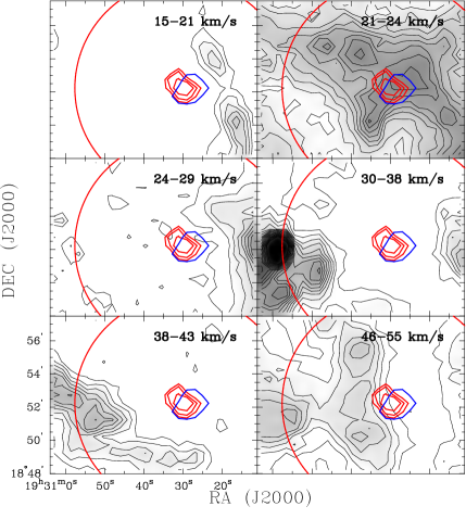
Fig. 2.—: ¹²CO $J$=2–1 integrated intensity maps showing individual velocity components at $v_{\rm LSR}\geq 15$ km s^-1. Integrated velocity ranges are marked on individual channel maps. Contour levels increase from 0.2 K km s^-1 in 0.2 K km s^-1 steps. The red contours show the 21-cm continuum brightness distribution of the central PWN of G54.1+0.3, while the blue contour shows the shape of the MIR shell at 70 $\mu$m. The large red circle of radius $6.^{\prime}5$ represents the outer boundary of the SNR blast wave (Lang et al. 2010; Bocchino et al. 2010). The pulsar PSR J1930+1852 is located at ($\alpha,\delta$)${}_{J2000}=$(19^h30^m30${}^{s}.13$,+18^∘52${}^{{}^{\prime}}$14${}^{{}^{\prime\prime}}.1).$

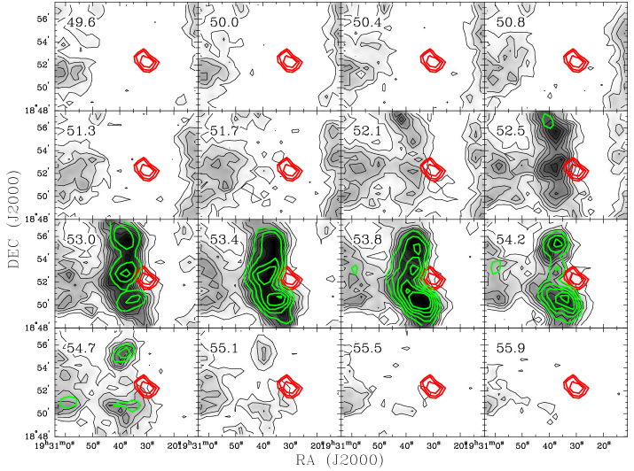
Fig. 3.—: ¹²CO $J$=2–1 channel maps of the +53 km s^-1 cloud. The contours have 0.4 K steps from 0.4 K. Again the red contours represent the PWN. The green contours show the ¹³CO distribution leveled from 0.4 K with 0.2 K steps.

3 RESULTS

3.1 Overall Distribution of CO Gas

Figure  1 shows the average spectrum of ¹²CO $J$ = 2–1 over the observed region with corresponding ¹³CO J = 1–0 spectrum obtained from the Galactic Ring Survey. Between $v_{LSR}$ = 0 and 60 km s^-1 distinct spectral components appear at 2, 8, 23, 32, 40 and 53 km s^-1 in the ¹²CO spectrum. In the bottom frame of the figure, we show the relation between the distance and LSR velocity according to the rotation curve of (Brand & Blitz 1993) which is close to the flat rotation curve with $R_{\odot}$ = 8.5 kpc and $\Theta_{\odot}$ = 220 km s^-1. Note that there are two distances corresponding to a given positive LSR velocity, i.e., +23 km s^-1 component could be either at 1.8 kpc or at 8.2 kpc. The maximum LSR velocity at this Galactic longitude (54.${}^{\circ}1$) is about 43 km s^-1 according to this model. But there are observations suggesting that the maximum rotation velocity toward this Galactic longitude is somewhat higher than 220 km s^-1 (see Leahy et al. 2008, and references therein), so that the +53 km s^-1 component might be near the tangential point which is 6.9 kpc assuming the above Galactocentric distance and Galactic rotational velocity at the Sun.

The integrated intensity maps at every 5–9 km s^-1 from 15 to 55 km s^-1 are presented in Figure  2. At $v_{LSR}$ = 15–21 km s^-1, there is a faint arc-like cloud elongated along the north-south direction in the western side of the PWN. As will be shown below, this arc-like cloud (hereafter $`$Arc Cloud’) has a large line width and systematic velocity gradient along the cloud. At $v_{LSR}$ = 21–24 km s^-1, there is strong, extended emission superposed on the PWN. It has a rather complex morphology with several peaks. Between $v_{LSR}$ = 24 and 43 km s^-1, CO clouds appear in the surrounding area, i.e., in the western and southeastern areas at 24–29 km s^-1 and 30–43 km s^-1, respectively. They are well separated from the PWN/IR-loop and extend beyond the SNR boundary, so that they are not considered to be possibly associated with the PWN (see §3.2). At 45–60 km s^-1, there is another thick, arc-like cloud that appears in contact with the eastern boundary of the PWN. This is the cloud that was proposed to be interacting with the PWN by Leahy et al. (2008). In the below, we first investigate the properties of the +53 km s^-1 component and then the +23 km s^-1 component.

3.2 +53 km s^-1 Cloud

Figure 3 shows channel maps of the +53 km s^-1 cloud where we overplot the contours of the ¹³CO 1–0 emission at corresponding velocities. The cloud is composed of three clumps of a few arc-minute extents; the southern brightest one centered at 53.9 km s^-1, a faint middle one at 53.5 km s^-1, and the northern one of moderate brightness at 54.3 km s^-1. The northern one is superposed with another filamentary cloud in the northern area at slightly lower velocity (52.6 km s^-1). As pointed out by Leahy et al. (2008), the PWN nebula is located in the middle where the cloud appears to kink. But we do not see any indication of the interaction in the line profiles of this cloud (Figure 4). The ratio ¹²CO(2–1)/¹³CO(1–0) ($\equiv R_{21/10}$)$\approx 5$ which is a typical value for a calm molecular cloud (e.g., see Sakamoto et al. 1994).

Fig. 4.—: Average ¹²CO $J=$2–1 (solid) and ¹³CO $J=$1–0 spectra (dotted) of (a) the 53 km s^-1 cloud and (b) the diffuse broad line emission in the eastern area of the cloud.

An interesting feature is the weak ($\sim 1$ K) emission between 45 and 55 km s^-1 in the eastern area of the +53 km s^-1 cloud. As shown in Figure 4, the CO line profiles are broad ($\sim 10$ km s^-1) although there seems to be more than one component. It extends beyond the eastern boundary of the our mapping area, so that we could not see its full extent. The association of this broad emission with the +53 km s^-1 cloud is not clear because the two clouds are connected by faint emission in the middle. Since the radio boundary of the G54.1+0.3 SNR appears quite circular and the broad emission extends beyond the boundary, we consider that this component is not related to the SNR. (The radio filaments outside the SNR shell shown in Figure 4 of Lang et al. (2010) are believed to be belong to a much larger-scale structure. See Figures 1–2 of Leahy et al. (2008).) Instead there is a star-forming infrared filament in the Spitzer MIPS 24 $\mu$m image that is spatially coincident with the broad CO emission as well as the 30–38 km s^-1 CO emission in Figure 2, and we suspect that the broad CO emission is associated with this filament.

3.3 +23 km s^-1 Clouds

The ¹²CO emission structure of the 23 km s^-1 cloud shown in Figure 5 is rather complicated, and it is helpful to look at the ¹³CO map first. In Figure 6, we show $R_{21/10}$ ratio map with the ¹³CO intensity contours overlaid. The ratios are derived in each channel for the pixels with $T_{mb,13}\geq 0.35$ K which corresponds to $5\sigma$ level. Note that the ratios are small where ¹³CO emission is strong. It becomes less than 1 at ¹³CO peaks. This is an indication of self-absorption by a relatively cold CO gas in front of warmer CO gas. The self-absorption is also apparent in the line profiles where we see a dip or a plateau in the ¹²CO profiles at which the ¹³CO intensity has maximum (Fig. 7). According to the ¹³CO intensity contour maps, the ¹³CO cloud at +23 km s^-1 is elongated along the northeast-southwest direction and is composed of several clumps. The clump that is spatially coincides with the PWN/IR-loop is the one in the southwestern end of the cloud. Its central velocity is 22.7 km s^-1, which is slightly smaller than those of the other clumps in the cloud. The median velocity of the ¹³CO cloud is $23.0\pm 0.2$ km s^-1.

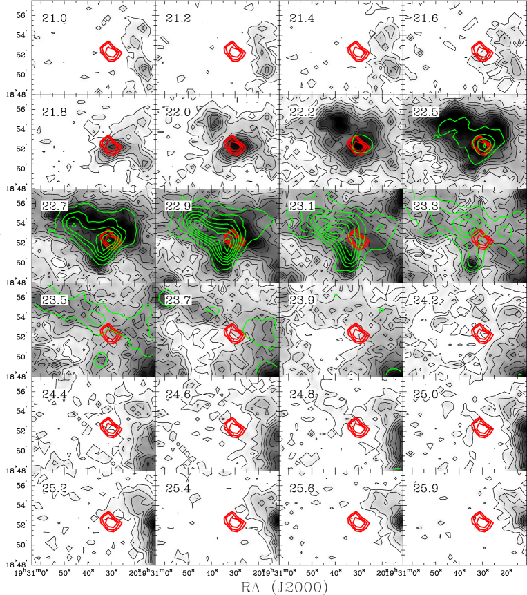
Fig. 5.—: Same as Fig. 3, but for the +23 km s^-1 cloud. ¹²CO contour levels increase from 0.4 K in 0.4 K steps.

The morphology of the +23 km s^-1 12CO cloud is now understandable. At 22.5–23.1 km s^-1, where the cloud is most apparent, the cloud has a ‘$\tau$’ shape, and the ¹³CO emission fits into the weak inner part of this structure. Therefore, the weak ¹²CO emission in the interior of ‘$\tau$’ shape should be mainly due to the absorption by the ¹³CO cloud. The self-absorption can be seen either when a cold CO cloud with high CO opacity but low excitation temperature is in front of warm CO gas further away, e.g., a cold cloud at 1.8 kpc aligned with a warm cloud at 8.2 kpc, or when a CO cloud has a temperature gradient along the line of sight. It is not unusual to see the self-absorption features in molecular clouds in the Galactic plane (e.g., Bieging et al. 2010). Considering the small angular sizes of the ¹²CO and ¹³CO clouds, the probability of a chance alignment of two clouds along the line of sight might be low. On the other hand, the self-absorption is prominent only to the eastern part of the ¹²CO cloud, which suggests that the absorbing ¹³CO cloud could be distinct from the ¹²CO cloud. But this could be due to the temperature and density structure of the cloud. In order to quantitatively understand the self-absorption features, we need to solve the radiative transfer equation together with statistical rate equations, which is beyond the scope of this paper.

The PWN/IR-loop spatially coincides with the southern part of the +23 km s^-1 cloud. There is no obvious indication of dynamical disruption in the line profile (see Fig. 8). There is a wing-like structure at high velocities (23–25 km s^-1), but this is likely due to other clouds in this area although it needs to be confirmed with an observation of higher angular resolution. But in the western part of the field, there are ¹²CO emissions with considerably large line widths, which are discussed in the next section.

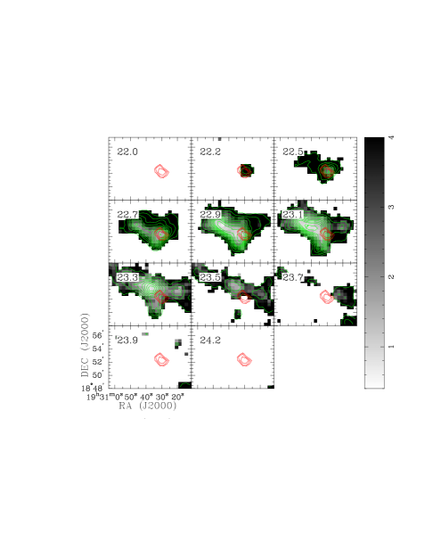
Fig. 6.—: ¹²CO(2–1)/¹³CO(1–0) ratio maps (grey scale) corresponding to the same channels in Fig. 5. The overlaid contours represent the ¹³CO intensities. The contours increase from 0.4 K in every 0.2 K steps.

Fig. 7.—: ¹²CO $J=$2–1(solid) and ¹³CO $J=$1–0 line profiles at positions where the self-absorption features are apparent. The positions of the spectra are marked in each frame with respect to (19^h30^m35.4^s,+18^∘52${}^{{}^{\prime}}$14${}^{{}^{\prime\prime}}$).

Fig. 8.—: Average ¹²CO $J=$2–1 (solid) and ¹³CO $J=$1–0 line profiles toward the position of the MIR loop.

3.4 Arc Cloud and Broad Line Molecular Gas at 15–30 km s^-1.

A distinct structure in the observed field is Arc Cloud seen in Figure 2 at velocities between 15 and 23 km s^-1 as an elongated cloud stretching over $5^{\prime}$ along the northeast-southwest direction. Along the structure, the ¹²CO line profiles have large line widths and their central velocities vary systematically as shown in Figures 9 and 10 which are the plot of spectra and position-velocity diagram along the arc structure. The systematic variation of the central velocity is clear; the velocity increases from 15 km s^-1 at the both ends of Arc Cloud to 23 km s^-1 at the middle point where the northern and southern arc structure merge. The velocity gradient is $\sim 8$ km s^-1  over 150^′′ from the middle to the north and south ends. At a distance of 8 kpc, it corresponds to $\sim 1.4$ km s^-1 pc^-1. The derived properties of Arc Cloud are summarized in Table 1. Velocity range is chosen as 15–22 km s^-1 to get the integrated intensity in Table 1 since the main cloud, some of which may not belong to Arc Cloud, starts to appear at $>22$ km s^-1. $\rm{T_{mb}}$ less than 0.4 K (several $\sigma$ level) was clipped out in the integration.

In addition to Arc Cloud, there are other broad lines at higher velocities in the northwestern area of the field. This can be seen, for example, in the line profiles of the northern part of Arc Cloud in Figure 9, but some representative line profiles are shown in Figure 11. In order to investigate the nature of the broad line emission, we fit the line profiles with 2 Gaussian components. Some profiles, i.e., the profiles with both the blue-shifted and red-shifted broad components, need three Gaussian components to describe the profiles correctly. But the two-component fit should be useful to see the basic properties of the broad components. We used MPFIT, which is a least-squares fitting tool based on the Levenberg-Marquardt algorithm (Markwardt 2009). In the fit, we leave the height, central velocity, and the width of individual components free with reasonable lower and upper boundaries.

Fig. 9.—: ¹²CO $J$=2–1 spectra along the (a) northern and (b) southern parts of Arc Cloud at every 30^′′ in declination. Note the broad-line component shifting systematically in velocity. Relative coordinates in arc-seconds from the map center are indicated in parentheses. The position angle in (a) is 45^∘ at the position of the bottom spectrum. Each spectrum is plotted with 2 K temperature offset. The vertical dashed lines are drawn just for velocity reference.

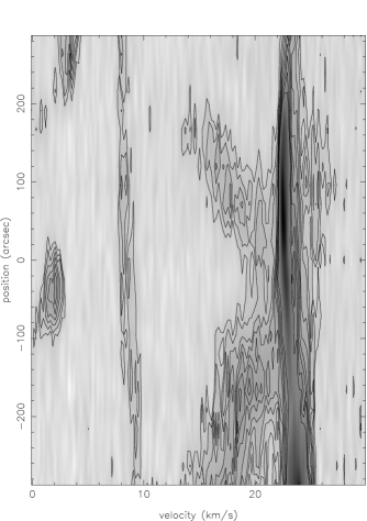
Fig. 10.—: Position-velocity diagram at the offset position ($\Delta\alpha,\Delta\delta$)$=($-230${}^{{}^{\prime\prime}}$,$0^{{}^{\prime\prime}}$) sliced in the position angle of 20 degrees. Contour levels increase from 0.4 K in 0.2 K steps. In order to show Arc Cloud clearly cutting position and angle are chosen dissimilar to Fig. 9. The southern part is brighter and more complex than the northern part.

Figure 12 shows the distributions of the height, central velocity, and width of the two Gaussian components. The height map of the first (narrow) component shows the morphology of the 23 km s^-1 component nicely. The second component represents the broad-line component, and its maps show that the broad-line component is confined to the western part of the field. In the central velocity map, we can identify Arc Cloud that has a velocity gradient that we described above. The broad-lines at higher velocities appear mainly to the western side of Arc Cloud. The very large width at the tip of the arc-like cloud indicates that, at those pixels, both blue-shifted and red-shifted velocity components appear (see Fig. 11). Figure 13 plots the line width versus central velocity of the two Gaussian components. The black dots confined to the central velocity of 23 km s^-1 and a width (FWHM) of 1.4 km s^-1 represents the first Gaussian component, or the +23 km s^-1 cloud component. The red dots represent the second Gaussian component, or the broad component, and they are scattered over the plane. The points with central velocities less than 20 km s^-1 might be from Arc Cloud while the points with widths greater than 7–8 km s^-1 have both red-shifted and blue-shifted broad components. Figure 13 shows that the broad lines in the western part of Arc Cloud have central velocities of 20–26 km s^-1 and widths of 2–7 km s^-1.

Table 1. : ¹²CO $J=$2–1 Line Properties of Arc Cloud

Center	(19h30m19s,+18∘52${}^{{}^{\prime}}$14${}^{{}^{\prime\prime}}$)
Length	$5^{\prime}$
Velocity range	15–23 km s-1
Velocity gradient	$\sim 3$ km s-1 arcmin-1
$\Delta v$(FWHM)	3.6 km s-1 –4.5 km s-1
Peak temperature	$\leq 1$ K
$\int T_{mb}dv$	$\sim 242$ K km s-1

Fig. 11.—: Some representative spectra showing broad line features. Their positions are marked in Fig. 12. The spectra at the bottom of each frame are the corresponding GRS ¹³CO $J$=1–0 spectra with -0.8 K offsets.

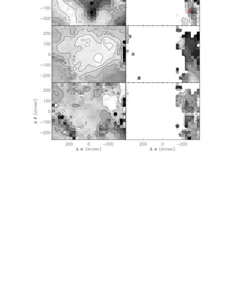
Fig. 12.—: Distribution of the parameters of two Gaussian components describing the line profiles between $v_{\rm LSR}=20$ and 28 km s^-1. The left column shows peak temperatures, central velocities, and line widths of narrow component while the right column shows the same plots for the broad lines. The positions of the spectra shown in Fig. 11 are marked in the top right panel.

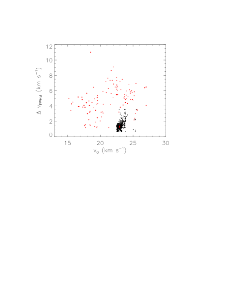
Fig. 13.—: Line width vs. central velocity of the two Gaussian components in Fig. 12. The narrow components (black dots) are confined to a small area with a central velocity of 23.1$\pm$0.24 km s^-1 and a median width of 0.58 km s^-1. On the other hand, the broad component(red dots) are scattered over a large area with a central velocity of $21.8\pm 6.2$ km s^-1 and a median width of 2.1 km s^-1. The areas of the circles are proportional to their heights.

4 Discussion and Conclusion

It has been previously proposed that the +23 km s^-1 and +53 km s^-1 molecular clouds are possibly associated with the SNR by Koo et al. (2008) and Leahy et al. (2008), respectively. They inspected the FCRAO ¹³CO survey data and found that those clouds have spatial correlation with the PWN, which led them to propose the association although there is no direct evidence for the interaction. Our ¹²CO $J$=2–1 map confirms the spatial correlation. The +23 km s^-1 component spatially coincides with the IR shell while the 53 km s^-1 component appears to be in contact with the eastern boundary of the PWN. The kinematic distances to these clouds are 1.8/8.2 kpc and 6.9 kpc, respectively. The distance to G54.1+0.3 has previously been determined in several studies. The distance based on HI absorption spectrum is from 5 to 10 kpc (Koo et al. 2008; Leahy et al. 2008), and the free-electron density/distance model (Cordes & Lazio 2002) gives the distance of $9^{+1.0}_{-1.5}$ kpc to the PSR J1930+1852 at the center of the PWN from its dispersion measure (Camilo et al. 2002). Recently, Kim et al. (2012) derived a distance of $6.0\pm 0.4$ kpc to the IR-excess stellar objects from a spectro-photometric study. Therefore, the estimated distance to the SNR ranges from 5 to 9 kpc, and in principle either of the cloud can be associated with the SNR.

The +53 km s^-1 cloud is composed of several arc-minute-sized clumps forming a kink-shaped structure (Fig. 3). The PWN is located in the middle where the cloud appears to kink. The spatial correlation is suggestive for the interaction as pointed out by Leahy et al. (2008). But we do not see any direct evidence of the interaction; its ¹²CO $J=$2–1 line profiles are well described by a single Gaussian with velocity widths (FWHM) of $1.5$–2.0 km s^-1. It is difficult to imagine a molecular cloud right at the SN explosion site but not disrupted. Also, the PWN shows no indication that it had encountered a dense medium only in the east; its radio structure has a east-west symmetry. Therefore, we consider that the association of the +53 km s^-1 cloud with the PWN is not likely. There is weak ($\sim 1$ K) diffuse emission with broad lines at comparable velocities in the eastern area of the cloud. The association of this diffuse component with the +53 km s^-1 cloud is uncertain. But since it extends beyond the radio boundary of the SNR, it is not likely that this component is associated with the SNR.

The 23 km s^-1 cloud has a complex structure with pronounced self-absorption features. The self-absorption could be either due to a foreground cold CO cloud along the line of sight or due to a temperature gradient in the cloud. The entire cloud structure is large ($\sim 10^{\prime}$) and again it is not likely that this cloud is associated with the SNR. There is a small clump in the southwestern end of the cloud that coincides with the MIR loop (Koo et al. 2008) at $\sim 22$ km s^-1 (see Fig. 5). It is not impossible that this clump is spatially separate from the +23 km s^-1 cloud, but there is no obvious indication of dynamical disruption in its line profile.

A distinct structure detected in this study is Arc Cloud in the west of the PWN at velocities between 15 and 23 km s^-1. The cloud is $5^{\prime}$ long and has a large line width. The central velocity increases from both ends of the cloud to the middle point systematically. The velocity at the end of the arc cloud is 15 km s^-1, so that the velocity shift from the middle (+23 km s^-1) is $\sim 8$ km s^-1. There are also other broad lines at higher velocities in the west of Arc Cloud. The association of this broad line emission with Arc Cloud is possible. It is interesting to note that the radio brightness of the SNR is relatively faint in its western part where these arc-like cloud and the broad-line clouds are located (see Fig. 4 of Lang et al. 2010). The SNR shock of G54.1+0.3 is currently expanding at $\sim 2,000$ km s^-1 and the density of the ambient medium is $\sim 0.2$ cm^-3 (Bocchino et al. 2010). If a dense molecular cloud is swept-up by this shock wave, the shock speed will drop by the square root of the density contrast. Therefore, Arc Cloud and the broad-line cloud could have been produced by the SNR shock if they were recently swept-up and if their densities were $\sim 10^{4}$ cm^-3. However in this part of the sky, there is a large star-forming molecular cloud near the Galactic plane at the same LSR velocity, but at a distance of 2 kpc. It is possible that the cloud that we observe is part of this cloud system. A further study is required to investigate their association.

In conclusion, we could not detect any direct evidence for the interaction of either the +53 or +23 km s^-1 cloud with the SNR from our CO $J=$2–1 line observations. Instead we have detected molecular gas with broad lines and with systematic velocity structure at $v_{\rm LSR}=$15–30 km s^-1 to the west of the IR loop but inside the SNR. Their association with the SNR needs to be investigated with further observations.

ACKNOWLEDGMENTS We express thanks to Yong-Sun Park, SRAO people and Do-Young Byun for support during commissioning of the new receiver system, especially Hyun-Woo Kang for update on control software. B.-C. K. and J.-E. L. have been supported by Basic Science Research Program NRF-2011-00007223 and 2012-0002330, respectively, through the National Research Foundation of Korea (NRF) funded by the Ministry of Education, Science and Technology. This publication makes use of molecular line data from the Boston University-FCRAO Galactic Ring Survey (GRS).

References

- Acciari et al. (2010) Acciari, V. A., Aliu, E., Arlen, T., et al. 2010, Discovery of Very High Energy -ray Emission from the SNR G54.1+0.3, ApJ, 719, L69
- Bieging et al. (2010) Bieging, J. H., Peters, W. L., & Kang, M. 2010, The Arizona Radio Observatory CO Mapping Survey of Galactic Molecular Clouds. I. The W51 Region in CO and 13CO J = 2-1 Emission, ApJS, 191, 232
- Bocchino et al. (2010) Bocchino, F., Bandiera, R., & Gelfand, J. 2010, XMM-Newton and SUZAKU detection of an X-ray emitting shell around the pulsar wind nebula G54.1+0.3, A&A, 520, A71
- Brand & Blitz (1993) Brand, J., & Blitz, L. 1993, The Velocity Field of the Outer Galaxy, A&A, 275, 67
- Camilo et al. (2002) Camilo, F., Lorimer, D. R., Bhat, N. D. R., Gotthelf, E. V., Halpern, J. P., Wang, Q. D., Lu, F. J., & Mirabal, N. 2002, Discovery of a 136 Millisecond Radio and X-Ray Pulsar in Supernova Remnant G54.1+0.3, ApJ, L71
- Cordes & Lazio (2002) Cordes, J. M.,& Lazio, T. J. W. 2002, “NE2001. I. A New Model for the Galactic Distribution of Free Electrons and its Fluctuations”; astro-ph/0207156
- Jackson et al. (2006) Jackson, J. M. et al. 2006, The Boston University-Five College Radio Astronomy Observatory Galactic Ring Survey, ApJS, 163, 145
- Kim et al. (2012) Kim, H.-J., Koo, B.-C., & Moon, D.-S. 2012, Near-infrared Spectroscopy of Infrared-Excess Stellar Objects in the Young Supernova Remnant G54.1+0.3 (to be submitted)
- Koo et al. (2008) Koo, B.-C., Mckee C. F., Lee, J.-J., Lee, H.-G., Lee, J.-E., & Moon, D.-S. 2008, A Massive-Star-forming Infrared Loop around the Crab-like Supernova Remnant G54.1+0.3: Post-Main-Sequence Triggered Star Formation?, ApJ, 673, L147
- Lang et al. (2010) Lang, C. C., Wang, Q. D., Lu, F., & Clubb, K. I. 2010, The Radio Properties and Magnetic Field Configuration in the Crab-like Pulsar Wind Nebula G54.1+0.3, ApJ, 709, 1125
- Leahy et al. (2008) Leahy, D. A., Tian, W., & Wang, Q. D. 2008, Distance Determination to the Crab-like Pulsar Wind Nebula G54.1+0.3 and the Search for its Supernova Remnant Shell, ApJ, 136, 1477
- Lee (2008) Lee, J.-W. 2008, Ph.D. thesis, Seoul National University
- Li et al. (2010) Li, H., Chen, Y., & Zhang, L. 2010, Lepto-hadronic origin of -rays from the G54.1+0.3 pulsar wind nebula, MNRAS, 408, L80
- Lu et al. (2002) Lu, F. J., Wang, Q. D., Asenbach, B., Durouchoux, P., & Song, L. M. 2002, Chandra Observation of Supernova Remnant G54.1+0.3: A Close Cousin of the Crab Nebula, ApJ, 568, L49
- Markwardt (2009) Markwardt, C. B. 2009, Non-linear Least-squares Fitting in IDL with MPFIT, Astronomical Data Analysis Software and Systems XVIII, 411, 251 (http://purl.com/net/mpfit)
- Sakamoto et al. (1994) Sakamoto, S., Hayashi, M., Hasegawa, T., Handa, T., & Oka, T. 1994, A large area CO ( = 2–1) mapping of the giant molecular clouds in Orion, ApJ, 425, 641
- Temim et al. (2010) Temim, T., Slane, P., Reynolds, S. P., Raymond, J. C., & Borkowski, K. J. 2010, Deep Chandra Observations of the Crab-like Pulsar Wind Nebula G54.1+0.3 and Spitzer Spectroscopy of the Associated Infrared Shell, ApJ, 710, 309