Harnack inequality for nondivergent parabolic operators on Riemannian manifolds

Abstract.

We consider second-order linear parabolic operators in non-divergence form that are intrinsically defined on Riemannian manifolds. In the elliptic case, Cabré proved a global Krylov-Safonov Harnack inequality under the assumption that the sectional curvature of the underlying manifold is nonnegative. Later, Kim improved Cabré’s result by replacing the curvature condition by a certain condition on the distance function. Assuming essentially the same condition introduced by Kim, we establish Krylov-Safonov Harnack inequality for nonnegative solutions of the non-divergent parabolic equation. This, in particular, gives a new proof for Li-Yau Harnack inequality for positive solutions to the heat equation in a manifold with nonnegative Ricci curvature.

1. Introduction and main results

In this paper, we study Harnack inequalities for solutions of second-order parabolic equations of non-divergence type on Riemannian manifolds. Let $(M,g)$ be a smooth, complete Riemannian manifold of dimension $n$. For $x\in M$ and $t\in\mathbb{R}$, let $A_{x,t}$ be a positive definite symmetric endomorphism of $T_{x}M$, where $T_{x}M$ is the tangent space of $M$ at $x$. We denote $\left\langle X,Y\right\rangle:=g(X,Y)$ and $\lvert X\rvert^{2}:=\left\langle X,X\right\rangle$ and assume that

(1) $$\lambda\lvert X\rvert^{2}\leq\left\langle A_{x,t}\,X,X\right\rangle\leq\Lambda|X|^{2},\quad\forall(x,t)\in M\times\mathbb{R},\quad\forall X\in T_{x}M$$

for some positive constants $\lambda$ and $\Lambda$. We consider a second-order, linear, uniformly parabolic operator $\mathscr{L}$ defined by

(2) $$\mathscr{L}u=Lu-u_{t}:=\mathrm{trace}(A_{x,t}\circ D^{2}u)-u_{t}\quad\mbox{in}\,\,\,M\times\mathbb{R},$$

where $\circ$ denotes composition of endomorphisms and $D^{2}u$ denotes the Hessian of the function $u$ defined by

$$D^{2}u\cdot X=\nabla_{X}\nabla u,$$

where $\nabla u(x)\in T_{x}M$ is the gradient of $u$ at $x$. Notice that in the special case when $A_{x,t}\equiv\mathrm{Id}$, the equation $\mathscr{L}u=0$ simply becomes the usual heat equation $u_{t}-\Delta u=0$.

In the elliptic setting, Cabré proved in a remarkable paper [Ca] that if the underlying manifold $M$ has nonnegative sectional curvature, then Krylov-Safonov type (elliptic) Harnack inequality holds for solutions of uniformly elliptic equations in non-divergence form. Later, Kim [K] improved Cabré’s result by removing the sectional curvature assumption and imposing a certain condition on distance function which, in the parabolic setting, should read as follows: For all $p\in M$, we have

(3) $$\triangle d_{p}(x) \leq\frac{n-1}{d_{p}(x)}\quad\mbox{for}\quad x\notin\operatorname{Cut}(p)\cup\{p\},$$

(4) $$Ld_{p}(x) \leq\frac{a_{L}}{d_{p}(x)}\quad\mbox{for}\quad x\notin\operatorname{Cut}(p)\cup\{p\},\quad t\in\mathbb{R},$$

where $d_{p}(x)=d(p,x)$ is the geodesic distance between $p$ and $x$, $\operatorname{Cut}(p)$ denotes the cut locus of $p$, and $a_{L}$ is some positive constant that is fixed by the operator $L$. We shall prove that if the above conditions (3) and (4) hold, then we have Krylov-Safonov Harnack inequality for the parabolic operator $\mathscr{L}$; i.e., if $u$ is a (smooth) nonnegative solution of $\mathscr{L}u=f$ in a cylinder $K_{2R}:=B_{2R}(x_{0})\times(t_{0}-4R^{2},t_{0})$, where $x_{0}\in M$ and $t_{0}\in\mathbb{R}$, then we have

(5) $$\sup_{K_{R}^{-}}u\leq C\left\{\inf_{K_{R}^{+}}u+R^{2}\left(\frac{1}{\operatorname{Vol}(K_{2R})}\int_{K_{2R}}\lvert f\rvert^{n+1}\right)^{\frac{1}{n+1}}\right\},$$

where $K_{R}^{-}:=B_{R}(x_{0})\times(t_{0}-3R^{2},t_{0}-2R^{2})$, $K_{R}^{+}:=B_{R}(x_{0})\times(t_{0}-R^{2},t_{0})$, $\operatorname{Vol}$ denotes the volume, and $C$ is a uniform constant depending only on $n,\lambda,\Lambda$ and $a_{L}$. It is well known that the condition (3) holds if the manifold $M$ has nonnegative Ricci curvature. Also, as it is proved in [K], the condition (4) is satisfied, for example, if for all $x\in M$ and any unit vector $e\in T_{x}M$, we have $\mathcal{M}^{-}[R(e)]\geq 0$. Here, $R(e)$ is the Ricci transformation of $T_{x}M$ into itself given by $R(e)X:=R(X,e)e$, where $R(X,Y)Z$ is the Riemannian curvature tensor, and

$$\mathcal{M}^{-}[R(e)]=\mathcal{M}^{-}[R(e),\lambda,\Lambda]:=\lambda\sum_{\kappa_{i}>0}\kappa_{i}+\Lambda\sum_{\kappa_{i}<0}\kappa_{i},$$

where $\kappa_{i}$ are eigenvalues of the (symmetric) endomorphism $R(e)$. In the case when $\mathscr{L}$ is the heat operator and $M$ has nonnegative Ricci curvature, then the condition $\mathcal{M}^{-}[R(e)]\geq 0$ is satisfied and thus the Harnack inequality (5) holds; i.e., if $M$ has nonnegative Ricci curvature, then we have

$$\sup_{K_{R}^{-}}u\leq C_{n}\left\{\inf_{K_{R}^{+}}u+R^{2}\left(\frac{1}{\operatorname{Vol}(K_{2R})}\int_{K_{2R}}\lvert u_{t}-\Delta u\rvert^{n+1}\right)^{\frac{1}{n+1}}\right\},$$

where $C_{n}$ is a constant that depends only on the dimension $n$. This, in particular implies the Harnack inequality of Li and Yau [LY]. Also, in the case when $M$ has nonnegative sectional curvature, then the condition $\mathcal{M}^{-}[R(e)]\geq 0$ is trivially satisfied and we have the inequality (5) with a constant $C$ depending only on $n,\lambda,\Lambda$, which especially reproduces the Harnack inequality by Krylov and Safonov [KS] in the Euclidean space.

One crucial ingredient in proving the Euclidean Krylov-Safonov Harnack inequality is the Krylov-Tso estimate, which is the parabolic counterpart of the Aleksandrov-Bakelman-Pucci (ABP) estimate. The Krylov-Tso estimate as well as the classical ABP estimate is proved using affine functions, which have no intrinsic interpretation in general Riemannian manifolds. In the elliptic case, Cabré ingeniously overcame this difficulty by replacing the affine functions by quadratic functions; quadratic functions have geometric meaning as the square of distance functions. Following Cabré’s approach, we introduce an intrinsically geometric version of Krylov-Tso normal map, namely,

$$\Phi(x,t):=\left(\exp_{x}\nabla_{x}u(x,t),-\frac{1}{2}d\left(x,\exp_{x}\nabla u(x,t)\right)^{2}-u(x,t)\right).$$

The map $\Phi$ is called the parabolic normal map related to $u(x,t)$. A few remarks are in order regarding the normal map. In the classical ABP (and Krylov-Tso) estimate, an affine function concerning with the (elliptic) normal map $x\mapsto\nabla u(x)$ plays a role to bound the maximum of $u$ by estimating the measure of the image of the normal map. Since an affine function cannot be generalized naturally to an intrinsic object in Riemannian manifolds, Cabré used paraboloids instead in [Ca]. The map

$$p\mapsto\min_{\Omega}\{u(x)-p\cdot x\}\quad\mbox{for a domain }\,\Omega$$

is considered (up to a sign) as the Legendre transform of $u$. Krylov [Kr] discovered the parabolic version of the Aleksandrov-Bakelman maximum principle and Tso [T] later simplified his proof by using the map

$$(x,t)\mapsto(\nabla_{x}u(x,t),\nabla_{x}u(x,t)\cdot x-u(x,t)).$$

We end the introduction by stating our main theorems. The rest of the paper shall be devoted to their proof. Below and hereafter, we denote

$$\fint_{Q}f:=\frac{1}{\operatorname{Vol}(Q)}\int_{Q}f$$

and

$$K_{r}(x_{0},t_{0}):=B_{r}(x_{0})\times(t_{0}-r^{2},t_{0}],\quad(x_{0},t_{0})\in M\times\mathbb{R}.$$

Theorem 1.1 (Harnack inequality).

Suppose conditions (3), (4) hold. Let $u$ be a nonnegative smooth function in $K_{2R}(x_{0},4R^{2})$, where $x_{0}\in M$ and $R>0$. Then, we have

(6) $$\sup_{K_{R}(x_{0},2R^{2})}u\leq C\left\{\inf_{K_{R}(x_{0},4R^{2})}u+R^{2}\left(\fint_{K_{2R}(x_{0},4R^{2})}\lvert\mathscr{L}u\rvert^{n+1}\right)^{\frac{1}{n+1}}\right\},$$

where $C$ is a uniform constant depending only on $n,\lambda,\Lambda$ and $a_{L}$.

Theorem 1.2 (Weak Harnack inequality).

Suppose the conditions (3), (4) hold. Let $u$ be a nonnegative smooth function satisfying $\mathscr{L}u\leq f$ in $K_{2R}(x_{0},4R^{2})$, where $x_{0}\in M$ and $R>0$. Then, we have

$$\left(\fint_{K_{R}(x_{0},2R^{2})}u^{p}\right)^{\frac{1}{p}}\leq C\left\{\inf_{K_{R}(x_{0},4R^{2})}u+R^{2}\left(\fint_{K_{2R}(x_{0},4R^{2})}\lvert f^{+}\rvert^{n+1}\right)^{\frac{1}{n+1}}\right\};\quad f^{+}:=\max(f,0),$$

where $p\in(0,1)$ and $C$ are uniform constants depending only on $n,\lambda,\Lambda$ and $a_{L}$.

2. Preliminaries

Let $(M,g)$ be a smooth, complete Riemannian manifold of dimension $n$, where $g$ is the Riemannian metric and $\operatorname{Vol}:=\operatorname{Vol}_{g}$ is the reference measure on $M$. We denote $\langle X,Y\rangle:=g(X,Y)$ and $|X|^{2}:=\langle X,X\rangle$ for $X,Y\in T_{x}M$, where $T_{x}M$ is the tangent space at $x\in M$. Let $d(\cdot,\cdot)$ be the distance function on $M$. For a given point $y\in M$, $d_{y}(x)$ denotes the distance function from $y$, i.e., $d_{y}(x):=d(x,y)$.

We recall the exponential map $\exp:TM\to M$. If $\gamma_{x,X}:{\mathbb{R}}\to M$ is the geodesic starting from $x\in M$ with velocity $X\in T_{x}M$, then the exponential map is defined by

$$\exp_{x}(X):=\gamma_{x,X}(1).$$

We note that the geodesic $\gamma_{x,X}$ is defined for all time since $M$ is complete. Given two points $x,y\in M$, there exists a unique minimizing geodesic $\exp_{x}(tX)$ joining $x$ to $y$ with $y=\exp_{x}(X)$ and we will write $X=\exp_{x}^{-1}(y)$.

For $X\in T_{x}M$ with $|X|=1$, we define

$$t_{c}(X):=\sup\left\{t>0:\exp_{x}(sX)\,\,\,\mbox{is minimizing between}\,\,\,x\,\,\,\mbox{and $\exp_{x}(tX)$}\right\}.$$

If $t_{c}(X)<+\infty$, $\exp_{x}(t_{c}(X)X)$ is a cut point of $x$. The cut locus of $x$ is defined as the set of all cut points of $x$, that is,

$$\operatorname{Cut}(x):=\left\{\exp_{x}(t_{c}(X)X):X\in T_{x}M\,\,\,\mbox{with $|X|=1,\,\,t_{c}(X)<+\infty$}\right\}.$$

Define

$$E_{x}:=\left\{tX\in T_{x}M:0\leq t<t_{c}(X),\,\,X\in T_{x}M\,\,\,\mbox{with $|X|=1$}\right\}\subset T_{x}M.$$

One can show that $\operatorname{Cut}(x)=\exp_{x}(\partial E_{x}),M=\exp_{x}(E_{x})\cup\operatorname{Cut}(x)$ and $\exp_{x}:E_{x}\to\exp_{x}(E_{x})$ is a diffeomorphism. We note that $\operatorname{Cut}(x)$ is closed and has measure zero. For any $x\notin\operatorname{Cut}(y)$ with $x\neq y$, then $d_{y}$ is smooth at $x$ and the Gauss lemma implies that

$$\nabla d_{y}(x)=-\frac{\exp_{x}^{-1}(y)}{|\exp_{x}^{-1}(y)|}$$

and

$$\nabla(d^{2}_{y}/2)(x)=-\exp_{x}^{-1}(y).$$

Let the Riemannain curvature tensor be defined by

$$R(X,Y)Z=\nabla_{X}\nabla_{Y}Z-\nabla_{Y}\nabla_{X}Z-\nabla_{[X,Y]}Z,$$

where $\nabla$ stands for the Levi-Civita connection. For a unit vector $e\in T_{x}M$, $R(e)$ will denote the Ricci transform of $T_{x}M$ into itself given by $R(e)X:=R(X,e)e$.

For $u\in C^{\infty}(M)$, the Hessian operator $D^{2}u(x):T_{x}M\to T_{x}M$ is defined by

$$D^{2}u(x)\cdot X=\nabla_{X}\nabla u(x).$$

Let $M$ and $N$ be Riemannian manifolds of dimension $n$ and $\phi:M\to N$ be smooth. The Jacobian of $\phi$ is the absolute value of determinant of the differential $d\phi$, i.e.,

$$\operatorname{Jac}\phi(x):=|\det d\phi(x)|\quad\mbox{for $x\in M$}.$$

We quote the following lemma from Lemma 3.2 in [Ca], in which the Jacobian of the map $x\mapsto\exp_{x}(\nabla v(x))$ is computed explicitly.

Lemma 2.1 (Cabré).

Let $v$ be a smooth function in an open set $\Omega$ of $M$. Define the map $\phi:\Omega\to M$ by

$$\phi(x):=\exp_{x}\nabla v(x).$$

Let $x\in\Omega$ and suppose that $\nabla v(x)\in E_{x}$. Set $y:=\phi(x)$. Then we have

$$\operatorname{Jac}\phi(x)=\operatorname{Jac}\exp_{x}(\nabla v(x))\cdot\Big{|}\det D^{2}\left(v+d^{2}_{y}/2\right)\left(x\right)\Big{|},$$

where $\operatorname{Jac}\exp_{x}(\nabla v(x))$ denotes the Jacobian of $\exp_{x}$, a map from $T_{x}M$ to $M$, at the point $\nabla v(x)\in T_{x}M$.

Under the condition (3), we have the estimate for Jacobian of the exponential map and Bishop’s volume comparison theorem as follows. We state the known results as a lemma. The proof can be found in [K, p. 286] (see also [L]).

Lemma 2.2.

Suppose that $M$ satisfies (3).

1. For any $x\in M$ and $X\in E_{x},$

   $$\operatorname{Jac}\exp_{x}(X)=|\det d\exp_{x}(X)|\leq 1.$$

2. (Bishop) For any $x\in M$, $\operatorname{Vol}(B_{R}(x))/R^{n}$ is nonincreasing with respect to $R$, where $B_{R}(x)$ is a geodesic ball of radius $R$ centered at $x$. Namely,

   $$\frac{\operatorname{Vol}(B_{R}(x))}{\operatorname{Vol}(B_{r}(x))}\leq\frac{R^{n}}{r^{n}}\quad\text{if $\,0<r<R$.}$$

   In particular, $M$ satisfies the volume doubling property; i.e., $\operatorname{Vol}(B_{2R}(x))\leq 2^{n}\operatorname{Vol}(B_{R}(x))$.

The following is the area formula, which follows easily from the area formula in Euclidean space and a partition of unity.

Lemma 2.3 (Area formula).

For any smooth function $\phi:M\times{\mathbb{R}}\to M\times{\mathbb{R}}$ and any measurable set $E\subset M\times{\mathbb{R}}$, we have

$$\int_{E}\operatorname{Jac}\phi(x,t)dV(x,t)=\int_{M\times{\mathbb{R}}}\mathcal{H}^{0}[E\cap\phi^{-1}(y,s)]dV(y,s),$$

where $\mathcal{H}^{0}$ is the counting measure.

Notation.

Let us summarize the notations and definitions that will be used.

• Let $r>0,\rho>0$, $z_{o}\in M$ and $t_{o}\in{\mathbb{R}}$. We denote

  $$K_{r,\,\rho}(z_{o},t_{o}):=B_{r}(z_{o})\times(t_{o}-\rho,t_{o}],$$

  where $B_{r}(z_{o})$ is a geodesic ball of radius $r$ centered at $z_{o}$.

• We denote $K_{r}(z_{o},t_{o}):=K_{r,\,r^{2}}(z_{o},t_{o})$.

• We say that a constant $C$ is uniform if $C$ depends only on $n,\lambda,\Lambda$ and $a_{L}$.

• We denote $\fint_{Q}f:=\frac{1}{\operatorname{Vol}(Q)}\int_{Q}f.$

• We denote $|Q|:=\operatorname{Vol}(Q)$.

• We denote the trace by $\operatorname{tr}$.

3. Key lemma

In this section, we obtain Aleksandrov-Bakelman-Pucci-Krylov-Tso type estimate (Lemma 3.2) for parabolic Harnack inequalities. We begin with direct computation of the Jacobian of the parabolic normal map $\Phi$ below, which is a parabolic analogue of Lemma 2.1.

Lemma 3.1.

Let $v$ be a smooth function in an open set $K$ of $M\times{\mathbb{R}}$. Define the map $\phi:K\to M$ by

$$\phi(x,t):=\exp_{x}\nabla_{x}v(x,t)$$

and the map $\Phi:K\rightarrow M\times{\mathbb{R}}$ by

$$\Phi(x,t):=\left(\phi(x,t),-\frac{1}{2}d\left(x,\phi(x,t)\right)^{2}-v(x,t)\right).$$

Let $(x,t)\in K$ and assume that $\nabla_{x}v(x,t)\in E_{x}.$ Set $y:=\phi(x,t).$ Then

$$\operatorname{Jac}\Phi(x,t)=\operatorname{Jac}\exp_{x}(\nabla_{x}v(x,t))\cdot\Big{|}(-v_{t})\det\left(D_{x}^{2}\left(v+d^{2}_{y}/2\right)\right)\Big{|},$$

where $\operatorname{Jac}\exp_{x}(\nabla_{x}v(x,t))$ denotes the Jacobian of $\exp_{x}$ at the point $\nabla_{x}v(x,t)\in T_{x}M$.

Proof.

We may assume that $\nabla_{x}v(x,t)\neq 0$, which is equivalent to $x\neq y$. Let $(\xi,\sigma)\in T_{x}M\times{\mathbb{R}}\backslash\{(0,0)\}$ and let $\gamma=(\gamma_{1},\gamma_{2})$ be the geodesic with $\gamma(0)=(x,t)$ and $\gamma^{\prime}(0)=(\xi,\sigma)$. We note that $\gamma_{1}(\tau)=\exp_{x}\tau\xi$ and $\gamma_{2}(\tau)=t+\sigma\tau$. Set

$$Y(s,\tau):=\exp_{\gamma_{1}(\tau)}\left[s\nabla_{x}v(\gamma(\tau))\right].$$

Consider the family of geodesics (in the parameter $s$)

$$\Pi(s,\tau):=\left(Y(s,\tau),\gamma_{2}(\tau)-s\left\{\frac{1}{2}d\left(\gamma_{1}(\tau),\phi(\gamma(\tau))\right)^{2}+\,v(\gamma(\tau))+\gamma_{2}(\tau)\right\}\right)$$

that joins $\Pi(0,\tau)=\gamma(\tau)$ to $\Pi(1,\tau)=\Phi(\gamma(\tau))$. Then we define

$$J(s):=\frac{\partial}{\partial\tau}\Big{|}_{\tau=0}\Pi(s,\tau),$$

which is a Jacobi field along

$$X(s):=\left(\exp_{x}(s\nabla_{x}v(x,t)),t-{\color[rgb]{0,0,0}s}\left\{\frac{1}{2}{d\left(x,\phi(x,t)\right)^{2}}+\,v(x,t)+t\right\}\right).$$

Simple computation says that

$${J(0)=(\xi,\sigma)}\quad\mbox{and}\quad J(1)=\frac{\partial}{\partial\tau}\Big{|}_{\tau=0}\Phi(\gamma(\tau))=d\Phi{(x,t)}\cdot(\xi,\sigma).$$

We also have

$$D_{s}J(0) =\left(D_{x}^{2}v(x,t)\,\xi+\sigma\nabla_{x}v_{t}(x,t)\right.,\quad-\sigma v_{t}(x,t)-\sigma$$

$$\left.-\left\langle\nabla_{x}\left(d_{x}^{2}/2\right)(y),\,d\exp_{x}(\nabla_{x}v(x,t))\cdot\left(D^{2}_{x}\left(v+d_{y}^{2}/2\right)(x,t)\cdot\xi+\sigma\nabla_{x}v_{t}(x,t)\right)\right\rangle\right).$$

In fact, we have

$$D_{s}J(0)=D_{s}\frac{\partial\Pi}{\partial\tau}\Big{|}_{s=0,\tau=0}=D_{\tau}\frac{\partial\Pi}{\partial s}\Big{|}_{s=0,\tau=0}$$

$$=D_{\tau}\Big{|}_{\tau=0}\left(\nabla_{x}v(\gamma(\tau)),-\frac{1}{2}d(\gamma_{1}(\tau),\phi(\gamma(\tau)))^{2}-v(\gamma(\tau))-\gamma_{2}(\tau)\right)$$

$$=\left(D^{2}_{x}v(x,t)\cdot\xi+\sigma\nabla_{x}v_{t}(x,t),\right.$$

$$\,\,-\left\langle\nabla_{x}(d_{y}^{2}/2)(x),\,\xi\right\rangle-\left.\left\langle\nabla_{x}(d_{x}^{2}/2)(\phi(x,t)),\frac{\partial}{\partial\tau}\phi(\gamma(\tau))\Big{|}_{\tau=0}\right\rangle-\left\langle\nabla_{x}v(x,t),\,\xi\right\rangle-\sigma v_{t}-\sigma\right)$$

$$=\left(D^{2}_{x}v\cdot\xi+\sigma\nabla_{x}v_{t},-\left\langle\nabla_{x}(d_{x}^{2}/2)(\phi(x,t)),\frac{\partial}{\partial\tau}\phi(\gamma(\tau))\Big{|}_{\tau=0}\right\rangle-\sigma v_{t}-\sigma\right),$$

since $\nabla_{x}(d^{2}_{y}/2)(x)=-\exp^{-1}_{x}(y)=-\nabla_{x}v(x,t)$. Then we use Lemma 2.1 to obtain

$$\frac{\partial}{\partial\tau}\phi(\gamma(\tau))\Big{|}_{\tau=0}=d\exp_{x}(\nabla_{x}v(x,t))\cdot\left(D_{x}^{2}\left(v+d_{y}^{2}/2\right)(x,t)\cdot\xi+\sigma\nabla_{x}v_{t}(x,t)\right).$$

On the other hand, consider the Jacobi field $J_{\xi,\sigma}$ along $X(s)$ satisfying

$$J_{\xi,\sigma}(0)=(\xi,\sigma)\quad\mbox{and}\quad J_{\xi,\sigma}(1)=(0,0).$$

Then we can check that

$$J_{\xi,\sigma}(s)=\frac{\partial}{\partial\tau}\Psi\Big{|}_{\tau=0}\quad\mbox{and}\quad D_{s}J_{\xi,\sigma}(0)=\left(-D^{2}_{x}\left(d_{y}^{2}/2\right)(x)\cdot\xi,-\sigma\right),$$

where

$$\Psi(s,\tau):=\left(\exp_{\gamma_{1}(\tau)}s\exp^{-1}_{\gamma_{1}(\tau)}\phi(x,t),\gamma_{2}(\tau)-s\left\{\frac{1}{2}d(x,\phi(x,t))^{2}+v(x,t)+\gamma_{2}(\tau)\right\}\right).$$

(We refer [Ca, Lemma 3.2] for the proof.)

Define $\tilde{J}_{\xi,\sigma}:=J-J_{\xi,\sigma}$. The Jacobi field $\tilde{J}_{\xi,\sigma}$ along $X(s)$ satisfying

$$\tilde{J}_{\xi,\sigma}(0)=(0,0)\quad\mbox{and}\quad D_{s}\tilde{J}_{\xi,\sigma}(0)=D_{s}J(0)-D_{s}J_{\xi,\sigma}(0)$$

is written by

$$d\exp_{(x,t)}(sX^{\prime}(0))\cdot\left(sD_{s}\tilde{J}_{\xi,\sigma}(0)\right).$$

Therefore, we have

$$J(1)=\tilde{J}_{\xi,\sigma}(1)=d\exp_{(x,t)}\left(\nabla_{x}v(x,t),-\frac{1}{2}d(x,y)^{2}-v(x,t)-t\right)\cdot\left(D_{s}J(0)-D_{s}J_{\xi,\sigma}(0)\right),$$

which means

$$d\Phi(x,t)\cdot(\xi,\sigma)=d\exp_{(x,t)}\left(\nabla_{x}v(x,t),-\frac{1}{2}d(x,y)^{2}-v(x,t)-t\right)\cdot$$

$$\left(D_{x}^{2}\left(v+d_{y}^{2}/2\right)(x,t)\cdot\xi+\sigma\nabla_{x}v_{t}(x,t)\,,\right.$$

$$\left.-\sigma v_{t}-\left\langle\nabla_{x}\left(d_{x}^{2}/2\right)(y),\,d\exp_{x}(\nabla_{x}v(x,t))\cdot\left(D^{2}_{x}\left(v+d_{y}^{2}/2\right)(x,t)\cdot\xi+\sigma\nabla_{x}v_{t}(x,t)\right)\right\rangle\right)$$

$$=\left(d\exp_{x}\left(\nabla_{x}v(x,t)\right)\cdot\left(D_{x}^{2}\left(v+d_{y}^{2}/2\right)(x,t)\cdot\xi+\sigma\nabla_{x}v_{t}(x,t)\right)\,,\right.$$

$$\left.-\sigma v_{t}-\left\langle\nabla_{x}\left(d_{x}^{2}/2\right)(y),\,d\exp_{x}(\nabla_{x}v(x,t))\cdot\left(D^{2}_{x}\left(v+d_{y}^{2}/2\right)(x,t)\cdot\xi+\sigma\nabla_{x}v_{t}(x,t)\right)\right\rangle\right).$$

To calculate the Jacobian of $\Phi$, we introduce an orthonormal basis $\{e_{1},\cdots,e_{n}\}$ of $T_{x}M$ and an orthonormal basis $\{\overline{e}_{1},\cdots,\overline{e}_{n}\}$ of $T_{y}M=T_{\exp_{x}\nabla v(x,t)}M$. By setting for $i,j=1,\cdots,n$,

$$A_{ij} :=\left\langle\overline{e}_{i},\,d\exp_{x}\left(\nabla_{x}v(x,t)\right)\cdot\left(D_{x}^{2}\left(v+d_{y}^{2}/2\right)(x,t)e_{j}\right)\right\rangle,$$

$$b_{i} :=\left\langle\overline{e}_{i},\,d\exp_{x}\left(\nabla_{x}v(x,t)\right)\cdot\nabla v_{t}(x,t)\right\rangle,$$

$$c_{i} :=\left\langle\overline{e}_{i},\,\nabla_{x}\left(d_{x}^{2}/2\right)(y)\right\rangle,$$

the Jacobian matrix of $\Phi$ at $(x,t)$ is

$$\left(\begin{array}[]{cc}A_{ij}&b_{i}\\ -c_{k}A_{kj}&-v_{t}-b_{k}c_{k}\end{array}\right).$$

Lastly, we use the row operations to deduce that

$$\operatorname{Jac}\Phi(x,t)=\left|\det\left(\begin{array}[]{cc}A_{ij}&b_{i}\\ 0&-v_{t}\end{array}\right)\right|=\left|(-v_{t})\det(A_{ij})\right|.$$

This completes the proof. ∎

The following lemma will play a key role to estimate sublevel sets of $u$ in Lemma 4.3 and then to prove a decay estimate of the distribution function of $u$ in Lemma 6.1. This ABP-type lemma corresponds to [Ca, Lemma 4.1].

Lemma 3.2.

Suppose that $M$ satisfies the condition (4). Let $z_{o}\in M$, $R>0$, and $0<\eta<1$. Let $u$ be a smooth function in $K_{\alpha_{1}R,\,\alpha_{2}R^{2}}(z_{o},0)\subset M\times{\mathbb{R}}$ satisfying

(7) $$u\geq 0\quad\mbox{in}\quad K_{\alpha_{1}R,\,\alpha_{2}R^{2}}(z_{o},0)\backslash K_{\beta_{1}R,\,\beta_{2}R^{2}}(z_{o},0)\quad\mbox{ and}\quad\inf_{K_{2R}(z_{o},0)}u\leq 1,$$

where $\alpha_{1}:=\frac{11}{\eta}$, $\alpha_{2}:=4+\eta^{2}+\frac{\eta^{4}}{4}$, $\beta_{1}:=\frac{9}{\eta}$, and $\beta_{2}:=4+\eta^{2}$. Then we have

(8) $$|B_{R}(z_{o})|\cdot R^{2}\leq C(\eta,n,\lambda)\int_{\{u\leq M_{\eta}\}\cap K_{\beta_{1}R,\,\beta_{2}R^{2}}(z_{o},0)}\left\{\left(R^{2}\mathscr{L}u+a_{L}+\Lambda+1\right)^{+}\right\}^{n+1}$$

where the constant $M_{\eta}>0$ depends only on $\eta>0$ and $C(\eta,n,\lambda)>0$ depends only on $\eta,n$ and $\lambda.$

Proof.

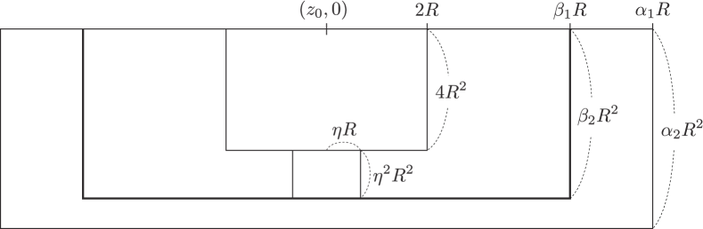
Figure 1. $\alpha_{1}:=\frac{11}{\eta},\alpha_{2}:=4+\eta^{2}+\frac{\eta^{4}}{4},\beta_{1}:=\frac{9}{\eta}$, $\beta_{2}:=4+\eta^{2}$.

For any $\overline{y}\in B_{R}(z_{o})$, we define

$$w_{\overline{y}}(x,t):=\frac{1}{2}R^{2}u(x,t)+\frac{1}{2}d_{\overline{y}}^{2}(x)-C_{\eta}t,\,\,\,\,C_{\eta}:=\frac{6}{\eta^{2}}.$$

From the assumption (7), it is easy to check that

$$\inf_{K_{2R}(z_{o},0)}w_{\overline{y}}\leq\left(5+\frac{24}{\eta^{2}}\right)R^{2}=:A_{\eta}R^{2},$$

and

$$w_{\overline{y}}\geq\left(6+\frac{24}{\eta^{2}}\right)R^{2}=(A_{\eta}+1)R^{2}\quad\mbox{on}\,\,\,K_{\alpha_{1}R,\,\alpha_{2}R^{2}}(z_{o},0)\backslash K_{\beta_{1}R,\,\beta_{2}R^{2}}(z_{o},0).$$

From the above observation, for any $\displaystyle(\overline{y},\overline{h})\in B_{R}(z_{o})\times\left(A_{\eta}R^{2},(A_{\eta}+1)R^{2}\right)$, we can find a time $\displaystyle\overline{t}\in\left(-\beta_{2}R^{2},0\right)$ such that

$$\overline{h}=\inf_{B_{\beta_{1}R}(z_{o})\times(-\beta_{2}R^{2},\overline{t}]}w_{\overline{y}}(z,\tau)=w_{\overline{y}}\left(\overline{x},\overline{t}\right),$$

where the infimum is achieved at an interior point $\overline{x}$ of $B_{\beta_{1}R}(z_{o})$. By the same argument as in [Ca, pp. 637-638], we have the following relation:

$$\overline{y}=\exp_{x}\nabla_{x}\left(\frac{1}{2}R^{2}u\right)\left(\overline{x},\overline{t}\right).$$

Now, we consider the map $\Phi:K_{\alpha_{1}R,\,\alpha_{2}R^{2}}(z_{o},0)\to M\times{\mathbb{R}}$ (with $v(x,t)=\frac{1}{2}R^{2}u(x,t)-C_{\eta}t$ in Lemma 3.1) defined as

$$\Phi(x,t):=\left(\exp_{x}\nabla_{x}\left(\frac{1}{2}R^{2}u\right)(x,t),-\frac{1}{2}d\left(x,\exp_{x}\nabla_{x}\left(\frac{1}{2}R^{2}u\right)(x,t)\right)^{2}-\frac{1}{2}R^{2}u(x,t)+C_{\eta}t\right).$$

Define a set

$$E:=\left\{(x,t)\in K_{\beta_{1}R,\,\beta_{2}R^{2}}(z_{o},0)\,:\,\exists y\in B_{R}(z_{o})\quad\mbox{s.t.}\quad\displaystyle w_{y}(x,t)=\inf_{B_{\beta_{1}R}(z_{o})\times(-\beta_{2}R^{2},t]}w_{y}\leq(A_{\eta}+1)R^{2}\,\right\}.$$

The set $E$ is a subset of the contact set in $K_{\beta_{1}R,\,\beta_{2}R^{2}}(z_{o},0)$ that contains a point $(x,t),$ where a concave paraboloid $-\frac{1}{2}d_{y}^{2}(x)+C_{\eta}t+C$ (for some $C$) touches $\frac{1}{2}R^{2}u$ from below. Thus we have proved that for any $(y,s)\in B_{R}(z_{o})\times(-(A_{\eta}+1)R^{2},-A_{\eta}R^{2})$, there is at least one $(x,t)\in E$ such that $(y,s)=\Phi(x,t)$, namely,

$$B_{R}(z_{o})\times\left(-(A_{\eta}+1)R^{2},-A_{\eta}R^{2}\right)\subset\Phi(E).$$

So Area formula gives

(9) $$|B_{R}(z_{o})|\cdot R^{2}\leq\int_{M\times{\mathbb{R}}}\mathcal{H}^{0}\left[E\cap\Phi^{-1}(y,s)\right]dV(y,s)=\int_{E}\operatorname{Jac}\Phi(x,t)dV(x,t).$$

We notice that for $(x,t)\in E$ and $y\in B_{R}(z_{o})$, $w_{y}(x,t)=\frac{1}{2}R^{2}u(x,t)+\frac{1}{2}d_{y}^{2}(x)-C_{\eta}t\leq(A_{\eta}+1)R^{2}$ and hence $u(x,t)\leq 2(A_{\eta}+1)=:M_{\eta}$ for $(x,t)\in E$.

Lastly, we claim that for $(x,t)\in E$,

(10) $$\operatorname{Jac}\Phi(x,t)\leq\frac{1}{(n+1)^{n+1}\lambda^{n}}\left\{\left(\frac{1}{2}R^{2}\mathscr{L}u(x,t)+a_{L}+\Lambda+C_{\eta}\right)^{+}\right\}^{n+1}.$$

Fix $(x,t)\in E$ and $y\in B_{R}(z_{o})$ to satisfy

$$w_{y}(x,t)=\inf_{B_{\beta_{1}R}(z_{o})\times(-\beta_{2}R^{2},t]}w_{y}.$$

We recall that $y=\exp_{x}\nabla_{x}\left(\frac{1}{2}R^{2}u\right)(x,t)$ (see [Ca, pp. 637-638]).

If $x$ is not a cut point of $y$, then Lemma 3.1 (with $v(x,t)=\frac{1}{2}R^{2}u(x,t)-C_{\eta}t$) and Lemma 2.2 (i) imply that

$$\operatorname{Jac}\Phi(x,t)\leq\left|\left(-\frac{1}{2}R^{2}u_{t}+C_{\eta}\right)\det\left(D_{x}^{2}\left(\frac{1}{2}R^{2}u+\frac{1}{2}d^{2}_{y}\right)\right)(x,t)\right|.$$

Since the minimum of $w_{y}$ in $B_{\beta_{1}R}(z_{o})\times(-\beta_{2}R^{2},t]$ is achieved at $(x,t)$, we have

$$0\leq D^{2}_{x}w_{y}(x,t)=D_{x}^{2}\left(\frac{1}{2}R^{2}u+\frac{1}{2}d^{2}_{y}\right)\,\,\,\mbox{and }\,\,\,0\geq\partial_{t}w_{y}(x,t)=\frac{1}{2}R^{2}u_{t}-C_{\eta},$$

where $D^{2}_{x}w_{y}(x,t)\geq 0$ means that the Hessian of $w_{y}$ at $(x,t)$ is positive semidefinite. Therefore, by using the geometric and arithmetic means inequality, we get

$$\operatorname{Jac}\Phi(x,t) \leq\left(-\frac{1}{2}R^{2}u_{t}+C_{\eta}\right)\det\left(D_{x}^{2}\left(\frac{1}{2}R^{2}u+\frac{1}{2}d^{2}_{y}\right)\right)(x,t)$$

$$\leq\frac{1}{\lambda^{n}}\left(-\frac{1}{2}R^{2}u_{t}+C_{\eta}\right)\det A_{x,t}\det\left(D_{x}^{2}\left(\frac{1}{2}R^{2}u+\frac{1}{2}d^{2}_{y}\right)\right)$$

$$\leq\frac{1}{(n+1)^{n+1}\lambda^{n}}\left\{\operatorname{tr}\left(A_{x,t}\circ D_{x}^{2}\left(\frac{1}{2}R^{2}u+\frac{1}{2}d^{2}_{y}\right)\right)-\frac{1}{2}R^{2}u_{t}+C_{\eta}\right\}^{n+1}$$

$$=\frac{1}{(n+1)^{n+1}\lambda^{n}}\left\{\frac{1}{2}R^{2}\mathscr{L}u(x,t)+L\left[\frac{1}{2}d^{2}_{y}\right]+C_{\eta}\right\}^{n+1}$$

$$\leq\frac{1}{(n+1)^{n+1}\lambda^{n}}\left\{\frac{1}{2}R^{2}\mathscr{L}u+a_{L}+\Lambda+C_{\eta}\right\}^{n+1}$$

$$=\frac{1}{(n+1)^{n+1}\lambda^{n}}\left\{\left(\frac{1}{2}R^{2}\mathscr{L}u+a_{L}+\Lambda+C_{\eta}\right)^{+}\right\}^{n+1},$$

where we used

$$L\left[d_{y}^{2}/2\right]=d_{y}Ld_{y}+\left<A_{x,t}\nabla d_{y},\nabla d_{y}\right>\leq a_{L}+\Lambda|\nabla d_{y}|^{2}.$$

When $x$ is a cut point of $y,$ we make use of upper barrier technique due to Calabi [Cal]. Since $y=\exp_{x}\nabla_{x}\left(\frac{1}{2}R^{2}u\right)(x,t)$, $x$ is not a cut point of $y_{\sigma}:=\phi_{\sigma}(x,t):=\exp_{x}\nabla_{x}\left(\frac{\sigma}{2}R^{2}u\right)(x,t)$ for $0\leq\sigma<1$. Now we consider

$$\Phi_{\sigma}(z,\tau):=\left(\phi_{\sigma}(z,\tau),-\frac{\sigma}{2}R^{2}u(z,\tau)-\frac{1}{2}d\left(z,\phi_{\sigma}(z,\tau)\right)^{2}+C_{\eta}\tau\right)$$

instead of $\Phi$ since $\displaystyle\operatorname{Jac}\Phi(x,t)=\lim_{\sigma\uparrow 1}\operatorname{Jac}\Phi_{\sigma}(x,t)$. As before, we have

$$\operatorname{Jac}\Phi_{\sigma}(x,t)\leq\left|\left(-\frac{\sigma}{2}R^{2}u_{t}+C_{\eta}\right)\det\left(D_{x}^{2}\left(\frac{\sigma}{2}R^{2}u+\frac{1}{2}d^{2}_{y_{\sigma}}\right)\right)(x,t)\right|.$$

We note that

$$\liminf_{\sigma\uparrow 1}\left|\left(-\frac{\sigma}{2}R^{2}u_{t}+C_{\eta}\right)\det\left(D_{x}^{2}\left(\frac{\sigma}{2}R^{2}u+\frac{1}{2}d^{2}_{y_{\sigma}}\right)\right)(x,t)\right|$$

$$= \liminf_{\sigma\uparrow 1}\left|\left(-\partial_{t}w_{y_{\sigma}}(x,t)\right)\det\left(D_{x}^{2}w_{y_{\sigma}}\right)(x,t)\right|$$

for $w_{y_{\sigma}}(z,\tau):=\frac{1}{2}R^{2}u(z,\tau)+\frac{1}{2}d_{y_{\sigma}}^{2}(z)-C_{\eta}\tau$. According to the triangle inequality, we have

$$w_{y}(z,\tau) \leq\frac{1}{2}R^{2}u(z,\tau)+\frac{1}{2}\left(d_{y_{\sigma}}(z)+d(y_{\sigma},y)\right)^{2}-C_{\eta}\tau$$

$$=w_{y_{\sigma}}(z,\tau)+d(y_{\sigma},y)d_{y_{\sigma}}(z)+\frac{1}{2}d(y_{\sigma},y)^{2},$$

where the equality holds at $(z,\tau)=(x,t)$. Since $w_{y}$ has the minimum at $(x,t)$ in $B_{\beta_{1}R}(z_{o})\times(-\beta_{2}R^{2},t]$, the minimum of $w_{y_{\sigma}}(z,\tau)+d(y_{\sigma},y)d_{y_{\sigma}}(z)$ (in $B_{\beta_{1}R}(z_{o})\times(-\beta_{2}R^{2},t]$) is also achieved at $(x,t)$, that implies that

$$D^{2}_{x}\left(w_{y_{\sigma}}+d(y_{\sigma},y)d_{y_{\sigma}}\right)(x,t)\geq 0,\quad\partial_{t}w_{y_{\sigma}}(x,t)\leq 0.$$

To bound $D^{2}y_{\sigma}(x)$ uniformly in $\sigma\in[1/2,1)$, we recall the Hessian comparison theorem (see [S],[SY]): Let $-k^{2}$ ($k>0$) be a lower bound of sectional curvature along the minimal geodesic joining $x$ and $y$. Then for $0<\sigma<1$,

$$D^{2}d_{y_{\sigma}}(x)\leq k\coth(kd_{y_{\sigma}}(x))\mathrm{Id}$$

and hence we find a constant $N>0$ independent of $\sigma$ such that

$$D^{2}d_{y_{\sigma}}(x)\leq N\mathrm{Id}\quad\mbox{for}\,\,\,\frac{1}{2}\leq\sigma<1.$$

Following the above argument, for $\frac{1}{2}\leq\sigma<1$, we obtain

$$0 \leq\liminf_{\sigma\uparrow 1}\left(-\partial_{t}w_{y_{\sigma}}(x,t)\right)\det\left(D_{x}^{2}w_{y_{\sigma}}+d(y_{\sigma},y)D^{2}d_{y_{\sigma}}\right)(x,t)$$

$$\leq\liminf_{\sigma\uparrow 1}\left(-\partial_{t}w_{y_{\sigma}}(x,t)\right)\det\left(D_{x}^{2}w_{y_{\sigma}}+d(y_{\sigma},y)N\mathrm{Id}\right)(x,t)$$

$$\leq\liminf_{\sigma\uparrow 1}\frac{1}{(n+1)^{n+1}\lambda^{n}}\left\{\frac{1}{2}R^{2}\mathscr{L}u+a_{L}+\Lambda+C_{\eta}+d(y_{\sigma},y)n\Lambda N\right\}^{n+1}$$

$$\leq\frac{1}{(n+1)^{n+1}\lambda^{n}}\left\{\left(\frac{1}{2}R^{2}\mathscr{L}u+a_{L}+\Lambda+C_{\eta}\right)^{+}\right\}^{n+1}.$$

Then we deduce that

$$\operatorname{Jac}\Phi(x,t)\leq\frac{1}{(n+1)^{n+1}\lambda^{n}}\left\{\left(\frac{1}{2}R^{2}\mathscr{L}u(x,t)+a_{L}+\Lambda+C_{\eta}\right)^{+}\right\}^{n+1}$$

since

$$\liminf_{\sigma\uparrow 1}\left|\det\left(D_{x}^{2}w_{y_{\sigma}}\right)(x,t)\right| =\liminf_{\sigma\uparrow 1}\left|\det\left(D_{x}^{2}w_{y_{\sigma}}+d(y_{\sigma},y)N\mathrm{Id}\right)(x,t)\right|$$

$$=\liminf_{\sigma\uparrow 1}\det\left(D_{x}^{2}w_{y_{\sigma}}+d(y_{\sigma},y)N\mathrm{Id}\right)(x,t).$$

We conclude that (10) is true for $(x,t)\in E.$ Therefore the estimate (8) follows from (9) since $E\subset\left\{u\leq M_{\eta}\right\}\cap K_{\beta_{1}R,\,\beta_{2}R^{2}}(z_{o},0)$. ∎

4. Barrier functions

We modify the barrier function of [W] to construct a barrier function in the Riemannian case. First, we fix some constants that will be used frequently (see Figure 1); for a given $0<\eta<1$,

$$\alpha_{1}:=\frac{11}{\eta},\,\alpha_{2}:=4+\eta^{2}+\frac{\eta^{4}}{4},\,\beta_{1}:=\frac{9}{\eta}\,\,\,\,\mbox{and}\,\,\,\beta_{2}:=4+\eta^{2}.$$

Lemma 4.1.

Suppose that $M$ satisfies the condition (4). Let $z_{o}\in M$, $R>0$ and $0<\eta<1$. There exists a continuous function $v_{\eta}(x,t)$ in $\displaystyle K_{\alpha_{1}R,\,\alpha_{2}R^{2}}(z_{o},\beta_{2}R^{2})$, which is smooth in $\left(M\backslash\operatorname{Cut}(z_{o})\right)\cap K_{\alpha_{1}R,\,\alpha_{2}R^{2}}(z_{o},\beta_{2}R^{2})$ such that

1. $v_{\eta}(x,t)\geq 0$ in $K_{\alpha_{1}R,\,\alpha_{2}R^{2}}(z_{o},\beta_{2}R^{2})\,\backslash\,K_{\beta_{1}R,\,\beta_{2}R^{2}}(z_{o},\beta_{2}R^{2})$,

2. $v_{\eta}(x,t)\leq 0$ in $K_{2R}(z_{o},\beta_{2}R^{2})$,

3. $R^{2}\mathscr{L}v_{\eta}+a_{L}+\Lambda+1\leq 0\$ a.e. in $K_{\beta_{1}R,\,\beta_{2}R^{2}}(z_{o},\beta_{2}R^{2})\backslash K_{\frac{\eta}{2}R}(z_{o},\frac{\eta^{2}}{4}R^{2}),$

4. $R^{2}\mathscr{L}v_{\eta}\leq C_{\eta}\quad a.e.$ in $K_{\beta_{1}R,\,\beta_{2}R^{2}}(z_{o},\beta_{2}R^{2})$,

5. $v_{\eta}(x,t)\geq-C_{\eta}$ in $K_{\alpha_{1}R,\,\alpha_{2}R^{2}}(z_{o},\beta_{2}R^{2})$.

Here, the constant $C_{\eta}>0$ depends only on $\eta,n,\lambda,\Lambda,a_{L}$ ( independent of $R$ and $z_{o}$ ).

Proof.

Fix $0<\eta<1$. Consider

$$h(s,t):=-Ae^{-mt}\left(1-\frac{s}{\beta_{1}^{2}}\right)^{l}\frac{1}{(4\pi t)^{n/2}}\exp\left(-\alpha\frac{s}{t}\right)\quad\mbox{for $t>0$,}$$

as in Lemma 3.22 of [W] and define

$$\psi(s,t):=h(s,t)+(a_{L}+\Lambda+1)t\quad\mbox{in $[0,\beta_{1}^{2}]\times[0,\beta_{2}]\backslash[0,\frac{\eta^{2}}{4}]\times[0,\frac{\eta^{2}}{4}]$, }$$

where the positive constants $A,m,l,\alpha$ ( depending only on $\eta,n,\lambda,\Lambda,a_{L}$) will be chosen later. In particular, $l$ will be an odd number in ${\mathbb{N}}$. We extend $\psi$ smoothly in $[0,\alpha_{1}^{2}]\times[-\frac{\eta^{4}}{4},\beta_{2}]$ to satisfy

$$\psi\geq 0\quad [0,\alpha_{1}^{2}]\times[-\frac{\eta^{4}}{4},\beta_{2}]\backslash[0,\beta_{1}^{2}]\times[0,\beta_{2}]$$ on ,

$$\psi\geq-C_{\eta}\quad [0,\alpha_{1}^{2}]\times[-\frac{\eta^{4}}{4},\beta_{2}]$$ on ,

and

$$\sup_{[0,\beta_{1}^{2}]\times[0,\beta_{2}]}\left\{2a_{L}\left|\partial_{s}\psi\right|+\Lambda\left(2|\partial_{s}\psi|+4s|\partial_{ss}\psi|\right)+|\partial_{t}\psi|\right\}(s,t)<C_{\eta}$$

for some $C_{\eta}>0$. We also assume that $\psi(s,t)$ is nondecreasing with respect to $s$ in $[0,\alpha_{1}^{2}]\times[-\frac{\eta^{4}}{4},\beta_{2}]$. We define

$$v_{\eta}(x,t)=v(x,t):=\psi\left(\frac{d^{2}_{z_{o}}(x)}{R^{2}},\frac{t}{R^{2}}\right)\quad\mbox{for }\,\,\,\,(x,t)\in K_{\alpha_{1}R,\,\alpha_{2}R^{2}}(z_{o},\beta_{2}R^{2}),$$

where $d_{z_{o}}$ is the distance function to $z_{o}$. Properties (i) and (v) are trivial.

We denote $d_{z_{o}}(x)$ and $h\left(\frac{d^{2}_{z_{o}}(x)}{R^{2}},\frac{t}{R^{2}}\right)$ by $d(x)$ and $\phi(x,t)$ for simplicity and we notice that for $(x,t)\in K_{\beta_{1}R,\,\beta_{2}R^{2}}(z_{o},\beta_{2}R^{2})\backslash K_{\frac{\eta}{2}R}(z_{o},\frac{\eta^{2}}{4}R^{2})$,

$$v(x,t) =h\left(\frac{d^{2}(x)}{R^{2}},\frac{t}{R^{2}}\right)+(a_{L}+\Lambda+1)\frac{t}{R^{2}}=\phi(x,t)+(a_{L}+\Lambda+1)\frac{t}{R^{2}}$$

and $\phi(x,t)$ is negative in $K_{\beta_{1}R,\,\beta_{2}R^{2}}(z_{o},\beta_{2}R^{2})$.

Now, we claim that

(11) $$\mathscr{L}\phi\leq 0\quad\mbox{a.e. in $K_{\beta_{1}R,\,\beta_{2}R^{2}}(z_{o},\beta_{2}R^{2})\backslash K_{\frac{\eta}{2}R}(z_{o},\frac{\eta^{2}}{4}R^{2})$.}$$

Once (11) is proved, then property (iii) follows from the simple calculation that $R^{2}\mathscr{L}\left[(a_{L}+\Lambda+1)\frac{t}{R^{2}}\right]=-(a_{L}+\Lambda+1)$ in $K_{\beta_{1}R,\beta_{2}R^{2}}(z_{o},\beta_{2}R^{2})$. Now we use the identity

$$\mathscr{L}[\varphi(u(x),t)]=\partial_{u}\varphi(u,t)\mathscr{L}u+\partial_{uu}\varphi(u,t)\langle A_{x,t}\nabla u,\nabla u\rangle-\partial_{t}\varphi(u,t)$$

to obtain

$$\mathscr{L}\phi =\frac{2d}{R^{2}}\partial_{s}h\left(\frac{d^{2}}{R^{2}},\frac{t}{R^{2}}\right)Ld$$

$$+\left\{\frac{2}{R^{2}}\partial_{s}h+\frac{4d^{2}}{R^{4}}\partial_{ss}h\right\}\left(\frac{d^{2}}{R^{2}},\frac{t}{R^{2}}\right)\langle A_{x,t}\nabla d,\nabla d\rangle-\frac{1}{R^{2}}\partial_{t}h\left(\frac{d^{2}}{R^{2}},\frac{t}{R^{2}}\right).$$

Since $d\cdot Ld\leq a_{L}$ and $\lambda\leq\langle A_{x,t}\nabla d,\nabla d\rangle\leq\Lambda$ in $M\backslash\operatorname{Cut}(z_{o}),$ we have that

$$\frac{(\beta_{1}^{2}R^{2}-d^{2})^{2}}{(-\phi)}\mathscr{L}\phi$$

$$=(\beta_{1}^{2}R^{2}-d^{2})\left\{2l+(\beta_{1}^{2}R^{2}-d^{2})\frac{2\alpha}{t}\right\}d\mathscr{L}d$$

$$-\left\{l(l-1)4d^{2}+2l(\beta_{1}^{2}R^{2}-d^{2})\frac{4\alpha d^{2}}{t}+(\beta_{1}^{2}R^{2}-d^{2})^{2}\frac{4\alpha^{2}d^{2}}{t^{2}}\right\}\langle A_{x,t}\nabla d,\nabla d\rangle$$

$$+(\beta_{1}^{2}R^{2}-d^{2})\left\{2l+(\beta_{1}^{2}R^{2}-d^{2})\frac{2\alpha}{t}\right\}\langle A_{x,t}\nabla d,\nabla d\rangle$$

$$+(\beta_{1}^{2}R^{2}-d^{2})^{2}\frac{\alpha d^{2}}{t^{2}}-(\beta_{1}^{2}R^{2}-d^{2})^{2}\left(\frac{n}{2t}+\frac{m}{R^{2}}\right)$$

$$\leq 2l(\beta_{1}^{2}R^{2}-d^{2})(a_{L}+\Lambda)+(\beta_{1}^{2}R^{2}-d^{2})^{2}\left\{\frac{2\alpha}{t}(a_{L}+\Lambda)+\frac{\alpha d^{2}}{t^{2}}\right\}$$

$$-l(l-1)4d^{2}\lambda-(\beta_{1}^{2}R^{2}-d^{2})^{2}\left(\frac{4\alpha^{2}d^{2}}{t^{2}}\lambda+\frac{n}{2t}\right)$$

$$-2l(\beta_{1}^{2}R^{2}-d^{2})\frac{4\alpha d^{2}}{t}\lambda-\frac{m}{R^{2}}(\beta_{1}^{2}R^{2}-d^{2})^{2}\quad\mbox{a.e. in $K_{\beta_{1}R,\,\beta_{2}R^{2}}(z_{o},\beta_{2}R^{2})$}.$$

By choosing

(12) $$\begin{split}\alpha&:=\frac{1}{4\lambda},\,\,\,\,\frac{2\beta_{1}^{2}}{\eta^{2}\lambda}(a_{L}+\Lambda)+1\leq l:=2l^{\prime}+1\,\,\,\mbox{(for some $l^{\prime}\in{\mathbb{N}}$)},\\ m&:=2\cdot\max\left\{\frac{8\alpha}{\eta^{2}}(a_{L}+\Lambda),\,\,\frac{2l(a_{L}+\Lambda)}{\beta_{1}^{2}-\frac{\eta^{2}}{4}}\right\},\end{split}$$

we deduce

$$\frac{(\beta_{1}^{2}R^{2}-d^{2})^{2}}{(-\phi)}\mathscr{L}\phi\leq 0\quad\mbox{a.e. in $K_{\beta_{1}R,\beta_{2}R^{2}}(z_{o},\beta_{2}R^{2})\backslash K_{\frac{\eta}{2}R}(z_{o},\frac{\eta^{2}}{4}R^{2})$.}$$

Indeed, we divide the domain $K_{\beta_{1}R,\beta_{2}R^{2}}(z_{o},\beta_{2}R^{2})\backslash K_{\frac{\eta}{2}R}(z_{o},\frac{\eta^{2}}{4}R^{2})$ into three regions such that

$$K_{\beta_{1}R,\beta_{2}R^{2}}(z_{o},\beta_{2}R^{2})\backslash K_{\frac{\eta}{2}R}(z_{o},\frac{\eta^{2}}{4}R^{2})=:A_{1}\cup A_{2}\cup A_{3},$$

where $A_{1}:=\{0\leq\frac{t}{R^{2}}\leq\frac{\eta^{2}}{4},\frac{\eta}{2}\leq\frac{d}{R}\leq\beta_{1}\},$ $A_{2}:=\{\frac{\eta^{2}}{4}\leq\frac{t}{R^{2}}\leq\beta_{2},\frac{\eta}{2}\leq\frac{d}{R}\leq\beta_{1}\}$ and $A_{3}:=\{\frac{\eta^{2}}{4}\leq\frac{t}{R^{2}}\leq\beta_{2},0\leq\frac{d}{R}\leq\frac{\eta}{2}\}$. We can check that

$$\frac{(\beta_{1}^{2}R^{2}-d^{2})^{2}}{(-\phi)}\mathscr{L}\phi\leq 0\quad\mbox{a.e. in $K_{\beta_{1}R,\beta_{2}R^{2}}(z_{o},\beta_{2}R^{2})\backslash K_{\frac{\eta}{2}R}(z_{o},\frac{\eta^{2}}{4}R^{2})$}$$

by choosing $\alpha$ and $l$ large in $A_{1}$, $m$ large in $A_{2}$ and $A_{3}$ as in (12). Therefore, we have proved (11).

From the assumption on $\psi$, we have that for a.e. $(x,t)\in K_{\beta_{1}R,\,\beta_{2}R^{2}}(z_{o},\beta_{2}R^{2})$,

$$R^{2}\mathscr{L}v(x,t) =2\partial_{s}\psi\left(\frac{d^{2}}{R^{2}},\frac{t}{R^{2}}\right)d\cdot Ld+\left\{2\partial_{s}\psi+\frac{4d^{2}}{R^{2}}\partial_{ss}\psi\right\}\left(\frac{d^{2}}{R^{2}},\frac{t}{R^{2}}\right)\langle A_{x,t}\nabla d,\nabla d\rangle$$

$$-\partial_{t}\psi\left(\frac{d^{2}}{R^{2}},\frac{t}{R^{2}}\right)$$

$$\leq\displaystyle\sup_{[0,\beta_{1}^{2}]\times[0,\beta_{2}]}\left\{2a_{L}{\partial_{s}\psi}+\Lambda\left(2\partial_{s}\psi+4s|\partial_{ss}\psi|\right)+|\partial_{t}\psi|\right\}(s,t)<C_{\eta}.$$

This proves property (iv).

In order to show (ii), we take $A>0$ large enough so that for $(x,t)\in K_{2R}(z_{o},\beta_{2}R^{2})$,

$$v(x,t) \leq-Ae^{-\beta_{2}m}\left(1-\frac{4}{\beta_{1}^{2}}\right)^{l}\frac{1}{{(4\pi\beta_{2})}^{n/2}}e^{-4\alpha/\eta^{2}}+(a_{L}+\Lambda+1)\beta_{2}\leq 0.$$

This finishes the proof of the lemma. ∎

Now we apply Lemma 3.2 to $u+v_{\eta}$ with $v_{\eta}$ constructed in Lemma 4.1 and translated in time. Since the barrier function $v_{\eta}(x,t)=\psi_{\eta}\left(\frac{d_{z_{o}}^{2}(x)}{R^{2}},\frac{t}{R^{2}}\right)$ is not smooth on $\operatorname{Cut}(z_{o})$, we need to approximate $v_{\eta}$ by a sequence of smooth functions as Cabré’s approach at [Ca]. We recall that the cut locus of $z_{o}$ is closed and has measure zero. It is not hard to verify the following lemma and we just refer to [Ca] Lemmas 5.3, 5.4.

Lemma 4.2.

Let $z_{o}\in M,\,R>0$ and let $\psi:{\mathbb{R}}^{+}\times[0,T]\to{\mathbb{R}}$ be a smooth function such that $\psi(s,t)$ is nondecreasing with respect to $s$ for any $t\in[0,T]$. Let $v(x,t):=\psi\left({d^{2}_{z_{o}}(x)},t\right)$. Then there exist a smooth function $0\leq\zeta(x)\leq 1$ on $M$ satisfying

$$\zeta\equiv 1\,\,\,\,\mbox{in $B_{\beta_{1}R}(z_{o})$ and }\,\,\,\,\operatorname{supp}\zeta\subset B_{\frac{10}{\eta}R}(z_{o})$$

and a sequence $\{w_{k}\}_{k=1}^{\infty}$ of smooth functions in $M\times[0,T]$ such that

$$\left\{\begin{array}[]{ll}w_{k}\to\zeta v&\mbox{uniformly in $M\times[0,T]$, }\\ \partial_{t}w_{k}\to\zeta\partial_{t}v&\mbox{uniformly in $M\times[0,T]$, }\\ D^{2}_{x}w_{k}\leq C\mathrm{Id}&\mbox{ in $M\times[0,T]$, }\\ D^{2}_{x}w_{k}\to D_{x}^{2}v&\mbox{a.e. in $B_{\beta_{1}R}(z_{o})\times[0,T]$, }\end{array}\right.\qquad\qquad$$

where the constant $C>0$ is independent of $k$.

Lemma 4.3.

Suppose that $M$ satisfies the conditions (3),(4). Let $z_{o}\in M,R>0$, and $0<\eta<1$. Let $u$ be a smooth function such that $\mathscr{L}u\leq f$ in $K_{\alpha_{1}R,\,\alpha_{2}R^{2}}(z_{o},4R^{2})$ such that

$$u\geq 0\quad\mbox{in}\quad K_{\alpha_{1}R,\,\alpha_{2}R^{2}}(z_{o},4R^{2})\backslash K_{\beta_{1}R,\,\beta_{2}R^{2}}(z_{o},4R^{2})$$

and

$$\inf_{K_{2R}(z_{o},4R^{2})}u\leq 1.$$

Then, there exist uniform constants $M_{\eta}>1,0<\mu_{\eta}<1$, and $0<\varepsilon_{\eta}<1$ such that

(13) $$\frac{\left|\left\{u\leq M_{\eta}\right\}\cap K_{\eta R}(z_{o},0)\right|}{\left|K_{\alpha_{1}R,\,\alpha_{2}R^{2}}(z_{o},4R^{2})\right|}\geq\mu_{\eta},$$

provided

(14) $$R^{2}\left(\fint_{K_{\alpha_{1}R,\,\alpha_{2}R^{2}}(z_{o},4R^{2})}|f^{+}|^{n+1}\right)^{\frac{1}{n+1}}\leq\varepsilon_{\eta},$$

where $M_{\eta}>0,\,0<\varepsilon_{\eta},\,\mu_{\eta}<1$ depend only on $\eta,n,\lambda,\Lambda$ and $a_{L}$.

Proof.

Let $v_{\eta}$ be the barrier function in Lemma 4.1 after translation in time (by $-\eta^{2}R^{2}$) and let $\{w_{k}\}_{k=1}^{\infty}$ be a sequence of smooth functions approximating $v_{\eta}$ as in Lemma 4.2. We notice that $u+v_{\eta}\geq 0$ in $K_{\alpha_{1}R,\,\alpha_{2}R^{2}}(z_{o},4R^{2})\backslash K_{\beta_{1}R,\,\beta_{2}R^{2}}(z_{o},4R^{2})$ and $\displaystyle\inf_{K_{2R}(z_{o},4R^{2})}(u+v_{\eta})\leq 1$. Thanks to the uniform convergence of $w_{k}$ to $\zeta v_{\eta}$, we consider a sequence $\{\varepsilon_{k}\}_{k=1}^{\infty}$ converging to $0$ such that $\displaystyle\sup_{K_{2R}(z_{o},4R^{2})}w_{k}\leq\varepsilon_{k}$ and

$$w_{k}\geq-\varepsilon_{k}\,\,\,\mbox{in}\,\,\,{K_{\alpha_{1}R,\,\alpha_{2}R^{2}}(z_{o},4R^{2})\backslash K_{\beta_{1}R,\,\beta_{2}R^{2}}(z_{o},4R^{2})},$$

and define

$$\overline{w}_{k}:=\frac{u+w_{k}+\varepsilon_{k}}{1+2\varepsilon_{k}}.$$

Then $\overline{w}_{k}$ satisfies the hypotheses of Lemma 3.2 (after translation in time by $4R^{2}$). Now we replace $u$ by $\overline{w}_{k}$ in (8) and then the uniform convergence implies that for a given $0<\delta<1$, we have

$$|B_{R}(z_{o})|R^{2} \leq C(\eta,n,\lambda)\int_{\{u+v_{\eta}\leq M_{\eta}+\delta\}\cap K_{\beta_{1}R,\,\beta_{2}R^{2}}(z_{o},4R^{2})}\left\{\left(R^{2}\mathscr{L}\overline{w}_{k}+a_{L}+\Lambda+1\right)^{+}\right\}^{n+1}$$

if $k$ is sufficiently large. Since $D_{x}^{2}w_{k}\leq C{\rm Id}$ and $|\partial_{t}w_{k}|<C$ uniformly in $k$ on $K_{\beta_{1}R,\beta_{2}R^{2}}(z_{o},4R^{2})$, we use the dominated convergence theorem to let $k$ go to $+\infty$. Letting $\delta$ go to $0$, we obtain

$$|B_{R}(z_{o})|\cdot R^{2} \leq C(\eta,n,\lambda)\int_{\{u+v_{\eta}\leq M_{\eta}\}\cap K_{\beta_{1}R,\beta_{2}R^{2}}(z_{o},4R^{2})}\left\{\left(R^{2}\mathscr{L}[u+v_{\eta}]+a_{L}+\Lambda+1\right)^{+}\right\}^{n+1}$$

$$=C(\eta,n,\lambda)\int_{E_{1}\cup E_{2}}\left\{\left(R^{2}\mathscr{L}[u+v_{\eta}]+a_{L}+\Lambda+1\right)^{+}\right\}^{n+1},$$

where $E_{1}:=\{u+v_{\eta}\leq M_{\eta}\}\cap\left(K_{\beta_{1}R,\,\beta_{2}R^{2}}(z_{o},4R^{2})\backslash K_{\eta R}(z_{o},0)\right)$ and $E_{2}:=\{u+v_{\eta}\leq M_{\eta}\}\cap K_{\eta R}(z_{o},0)$. From properties (iii) and (iv) of $v_{\eta}$ in Lemma 4.1 and Bishop’s volume comparison theorem in Lemma 2.2, we deduce that

$${|K_{\alpha_{1}R,\,\alpha_{2}R^{2}}(z_{o},4R^{2})|^{\frac{1}{n+1}}} \leq C_{\eta}\left\|\left(R^{2}\mathscr{L}u\right)^{+}\right\|_{L^{n+1}\left(K_{\beta_{1}R,\beta_{2}R^{2}}(z_{o},4R^{2})\right)}+C_{\eta}\left\|\chi_{E_{2}}\right\|_{L^{n+1}\left(K_{\beta_{1}R,\,\beta_{2}R^{2}}(z_{o},4R^{2})\right)}$$

$$\leq C_{\eta}||R^{2}f^{+}||_{L^{n+1}\left(K_{\alpha_{1}R,\,\alpha_{2}R^{2}}(z_{o},4R^{2})\right)}+C_{\eta}\left|\left\{u+v_{\eta}\leq M_{\eta}\right\}\cap K_{\eta R}(z_{o},0)\right|^{\frac{1}{n+1}},$$

where $C_{\eta}>0$ depends only on $n,\lambda$ and $\eta>0$. We note that $\{u\leq M_{\eta}-v_{\eta}\}\subset\{u\leq M_{\eta}+C_{\eta}\}$ from (v) in Lemma 4.1. Therefore, by taking

$$\varepsilon_{\eta}=\frac{1}{2C_{\eta}},\,\,\,M^{\prime}_{\eta}=M_{\eta}+C_{\eta}\,\,\,\,\mbox{and}\,\,\,\,\mu_{\eta}^{\frac{1}{n+1}}=\frac{1}{2C_{\eta}},$$

we conclude that $\displaystyle\frac{\left|\left\{u\leq M^{\prime}_{\eta}\right\}\cap K_{\eta R}(z_{o},0)\right|}{\left|K_{\alpha_{1}R,\,\alpha_{2}R^{2}}(z_{o},4R^{2})\right|}\geq\mu_{\eta}>0.$∎

Using iteration of Lemma 4.3, we have the following corollaries.

Corollary 4.4.

Suppose that $M$ satisfies the conditions (3),(4). Let $z_{o}\in M$ and $0<\eta<1$. For $i\in{\mathbb{N}}$, let $\overline{R}_{i}:=\left(\frac{2}{\eta}\right)^{i-1}R$ and $\overline{t}_{i}:=\sum_{j=1}^{i}4\overline{R}_{j}^{2}$. Let $u$ be a nonnegative smooth function such that $\mathscr{L}u\leq f$ in $\bigcup_{i=1}^{k}K_{\alpha_{1}\overline{R}_{i},\alpha_{2}\overline{R}_{i}^{2}}(z_{o},\overline{t}_{i})$ for some $k\in{\mathbb{N}}$. We assume that for $h>0$, $\displaystyle\inf_{\bigcup_{i=1}^{k}K_{2\overline{R}_{i}}(z_{o},\overline{t}_{i})}u\leq h$ and

$$\overline{R}_{i}^{2}\left(\fint_{K_{\alpha_{1}\overline{R}_{i},\alpha_{2}\overline{R}_{i}^{2}}(z_{o},\overline{t}_{i})}|f^{+}|^{n+1}\right)^{\frac{1}{n+1}}\leq\varepsilon_{\eta}hM_{\eta}^{k-i},\,\,\,\forall 1\leq i\leq k.$$

Then we have

(15) $$\frac{\left|\left\{u\leq hM^{k}_{\eta}\right\}\cap K_{\eta R}(z_{o},0)\right|}{\left|K_{\alpha_{1}R,\,\alpha_{2}R^{2}}(z_{o},4R^{2})\right|}\geq\mu_{\eta},$$

where $M_{\eta},\varepsilon_{\eta},\mu_{\eta}$ are the same uniform constants as in Lemma 4.3.

Proof.

We may assume $h=1$ since $v:=\frac{u}{h}$ satisfies $\mathscr{L}v=\frac{1}{h}\mathscr{L}u\leq\frac{f}{h}$. We use the induction on $k$ to show the lemma. When $k=1$, it is immediate from Lemma 4.3.

Now suppose that (15) is true for $k-1$. By assumption, we find a $j_{o}\in{\mathbb{N}}$ such that $1\leq j_{o}\leq k$ and $\displaystyle\inf_{K_{2\overline{R}_{j_{o}}}(z_{o},\overline{t}_{j_{o}})}u=\inf_{\bigcup_{i=1}^{k}K_{2\overline{R}_{i}}(z_{o},\overline{t}_{i})}u\leq 1$. Define $v:={u}/{M^{k-j_{o}}_{\eta}}$. Then $v$ satisfies that $\displaystyle\mathscr{L}v\leq{f}/{M^{k-j_{o}}_{\eta}},\,\inf_{K_{2\overline{R}_{j_{o}}}(z_{o},\overline{t}_{j_{o}})}v\leq 1$ and

$$\overline{R}_{j_{o}}^{2}\left(\fint_{K_{\alpha_{1}\overline{R}_{j_{o}},\,\alpha_{2}\overline{R}_{j_{o}}^{2}}(z_{o},\overline{t}_{j_{o}})}\left|f^{+}/M^{k-j_{o}}_{\eta}\right|^{n+1}\right)^{\frac{1}{n+1}}\leq\varepsilon_{\eta}.$$

Applying Lemma 4.3 to $v$ in $K_{\alpha_{1}\overline{R}_{j_{o}},\,\alpha_{2}\overline{R}_{j_{o}}^{2}}(z_{o},\overline{t}_{j_{o}})$, we deduce

$$\frac{\left|\left\{v\leq M_{\eta}\right\}\cap K_{\eta\overline{R}_{j_{o}}}(z_{o},\overline{t}_{j_{o}}-4R_{j_{o}}^{2})\right|}{\left|K_{\alpha_{1}\overline{R}_{j_{o}},\,\alpha_{2}\overline{R}_{j_{o}}^{2}}(z_{o},\overline{t}_{j_{o}})\right|}=\frac{\left|\left\{v\leq M_{\eta}\right\}\cap K_{2\overline{R}_{j_{o}-1}}(z_{o},\overline{t}_{j_{o}-1})\right|}{\left|K_{\alpha_{1}\overline{R}_{j_{o}},\,\alpha_{2}\overline{R}_{j_{o}}^{2}}(z_{o},\overline{t}_{j_{o}})\right|}\geq\mu_{\eta}>0$$

which implies that $\displaystyle\inf_{\bigcup_{i=1}^{j_{o}-1}K_{2\overline{R}_{i}}(z_{o},\overline{t}_{i})}u\leq\inf_{K_{2\overline{R}_{j_{o}-1}}(z_{o},\overline{t}_{j_{o}-1})}u\leq M^{k-j_{o}+1}_{\eta}$. Therefore, we use the induction hypothesis for $j_{o}-1(\leq k-1)$ to conclude

$$\frac{\left|\left\{u/M_{\eta}^{k-j_{o}+1}\leq M^{j_{o}-1}_{\eta}\right\}\cap K_{\eta R}(z_{o},0)\right|}{\left|K_{\alpha_{1}R,\,\alpha_{2}R^{2}}(z_{o},4R^{2})\right|}\geq\mu_{\eta}>0,$$

which implies (15). ∎

We remark that Lemma 4.3 and Corollary 4.4 hold for any $M^{\prime}_{\eta}\geq M_{\eta}$. The following is a simple technical lemma that will be used in the proof of Proposition 4.6.

Lemma 4.5.

Let $A,D>0$ and $\varepsilon>0$. Let $u$ be a nonnegative smooth function such that $\mathscr{L}u\leq f$ in $\overline{B_{R}(z_{o})}\times(-AR^{2},0]$ with

$$R^{2}\left(\fint_{B_{R}(z_{o})\times(-AR^{2},0]}|f^{+}|^{n+1}\right)^{\frac{1}{n+1}}\leq\varepsilon.$$

Then, there exists a sequence $u_{k}$ of nonnegative smooth functions in $B_{R}(z_{o})\times(-AR^{2},DR^{2}]$ such that $u_{k}$ converges to $u$ locally uniformly in $B_{R}(z_{o})\times(-AR^{2},0]$ and $\mathscr{L}u_{k}\leq g_{k}$ in $B_{R}(z_{o})\times(-AR^{2},DR^{2}]$ with

$$R^{2}\left(\fint_{B_{R}(z_{o})\times(-AR^{2},DR^{2}]}|g_{k}^{+}|^{n+1}\right)^{\frac{1}{n+1}}\leq\varepsilon.$$

Proof.

First, we define for $(x,t)\in B_{R}(z_{o})\times(-\infty,DR^{2}]$,

$$\overline{u}(x,t):=\left\{\begin{array}[]{ll}0&\mbox{for $\,\,t\in(-\infty,-AR^{2}]$, }\\ u(x,t)&\mbox{for $\,\,t\in(-AR^{2},0]$, }\\ u(x,0)+St&\mbox{for $\,\,t\in(0,DR^{2}]$},\end{array}\right.\qquad\qquad$$

where $\displaystyle S:=\sup_{B_{R}(z_{o})}\left\{(\mathscr{L}u)^{+}(x,0)+|u_{t}(x,0)|\right\}$. Then $\overline{u}$ is Lipschitz continuous with respect to time in $B_{R}(z_{o})\times(-AR^{2},DR^{2}]$ and satisfies

$$\mathscr{L}\overline{u}(x,t)\leq\overline{f}(x,t):=\left\{\begin{array}[]{ll}0&\mbox{for $t\in(-\infty,-AR^{2})$, }\\ f(x,t)&\mbox{for $t\in(-AR^{2},0)$, }\\ \mathscr{L}u(x,0)+u_{t}(x,0)-S\leq 0&\mbox{for $t\in(0,DR^{2}]$}.\end{array}\right.\qquad\qquad$$

Let $\varepsilon_{k}>0$ converge to $0$ as $k\to+\infty,$ and let $\varphi$ be a nonnegative smooth function such that $\varphi(t)=0$ for $t\not\in(0,1)$ and $\int_{\mathbb{R}}\varphi(t)dt=1$. We define $\displaystyle\varphi_{k}(t):=\frac{1}{\varepsilon_{k}}\varphi\left(\frac{t}{\varepsilon_{k}}\right)$ and

$$u_{k}(x,t):=\int_{\mathbb{R}}\overline{u}(x,s)\varphi_{k}(t-s)ds,\,\,\,\forall(x,t)\in B_{R}(z_{o})\times(-\infty,DR^{2}],$$

where we notice that the above integral is calculated over $(t-\varepsilon_{k},t)\subset{\mathbb{R}}$. Then, a smooth function $u_{k}$ satisfies

$$\mathscr{L}u_{k}(x,t)=\int_{\mathbb{R}}\mathscr{L}\overline{u}(x,s)\varphi_{k}(t-s)ds\leq g_{k}(x,t),\quad\mbox{$\forall(x,t)\in B_{R}(z_{o})\times(-\infty,DR^{2}],$ }$$

where $g_{k}(x,t):=\displaystyle\int_{\mathbb{R}}\overline{f}^{+}(x,s)\varphi_{k}(t-s)ds\geq 0$. We also have

$$R^{2}\left(\fint_{B_{R}(z_{o})\times(-AR^{2},DR^{2}]}|g_{k}^{+}|^{n+1}\right)^{\frac{1}{n+1}} \leq\frac{R^{2}}{\left\{|B_{R}(z_{o})|\cdot(A+D)R^{2}\right\}^{\frac{1}{n+1}}}||\overline{f}^{+}||_{L^{n+1}\left(B_{R}(z_{o})\times(-AR^{2}-\varepsilon_{k},DR^{2}-\varepsilon_{k}]\right)}$$

$$\leq\frac{R^{2}}{\left\{|B_{R}(z_{o})|\cdot(A+D)R^{2}\right\}^{\frac{1}{n+1}}}||\overline{f}^{+}||_{L^{n+1}\left(B_{R}(z_{o})\times(-AR^{2},0]\right)}$$

$$\leq\left(\frac{A}{A+D}\right)^{\frac{1}{n+1}}\varepsilon<\varepsilon,$$

which finishes the proof. ∎

Proposition 4.6.

Suppose that $M$ satisfies the conditions (3),(4). Let $z_{o}\in M,R>0,0<\eta<\frac{1}{2}$ and $\tau\in[3,16].$ Let $u$ be a nonnegative smooth function such that $\mathscr{L}u\leq f$ in $B_{\frac{49}{\eta^{3}}R}(z_{o})\times\left(-3R^{2},\frac{\tau R^{2}}{\eta^{2}}\right]$. Assume that $\displaystyle\inf_{B_{R}(z_{o})\times\left[\frac{2R^{2}}{\eta^{2}},\frac{\tau R^{2}}{\eta^{2}}\right]}u\leq 1$ and

$$R^{2}\left(\fint_{B_{\frac{49}{\eta^{3}}R}(z_{o})\times\left(-3R^{2},\frac{\tau R^{2}}{\eta^{2}}\right]}|f^{+}|^{n+1}\right)^{\frac{1}{n+1}}\leq\varepsilon^{\prime}_{\eta}$$

for a uniform constant $0<\varepsilon^{\prime}_{\eta}<1.$ Let $r>0$ satisfy $\left(\frac{\eta}{2}\right)^{N}R\leq r<\left(\frac{\eta}{2}\right)^{N-1}R$ for some $N\in{\mathbb{N}}$ and let $(z_{1},t_{1})$ be a point such that $d(z_{o},z_{1})<R$ and $|t_{1}|<R^{2}$. Then there exists a uniform constant $M^{\prime}_{\eta}>1$ (independent of $r,N,z_{1}$ and $t_{1}$) such that

$$\frac{\left|\left\{u\leq{M^{\prime}_{\eta}}^{N+2}\right\}\cap K_{\eta r}(z_{1},t_{1})\right|}{\left|K_{\alpha_{1}r,\,\alpha_{2}r^{2}}(z_{1},t_{1}+4r^{2})\right|}\geq\mu_{\eta}>0,$$

where $0<\mu_{\eta}<1$ is the constant in Lemma 4.3.

Proof.

(i) From Lemma 4.5, we approximate $u$ by nonnegative smooth functions $u_{k},$ which are defined on $B_{\frac{48}{\eta^{3}}R}(z_{o})\times\left(-3R^{2},\frac{64R^{2}}{(4-\eta^{2})\eta^{6}}+R^{2}\right].$ We find functions $u_{k}$ and $g_{k}$ such that $u_{k}$ converges locally uniformly to $u$ in $B_{\frac{48}{\eta^{3}}R}(z_{o})\times\left(-3R^{2},\frac{\tau R^{2}}{\eta^{2}}\right],$ and satisfies

$$\mathscr{L}u_{k}\leq g_{k}\quad\mbox{in}\,\,\,B_{\frac{48}{\eta^{3}}R}(z_{o})\times\left(-3R^{2},\frac{64R^{2}}{(4-\eta^{2})\eta^{6}}+R^{2}\right],$$

and

$$R^{2}\left(\fint_{B_{\frac{48}{\eta^{3}}R}(z_{o})\times\left(-3R^{2},\frac{64R^{2}}{(4-\eta^{2})\eta^{6}}+R^{2}\right]}|g_{k}^{+}|^{n+1}\right)^{\frac{1}{n+1}}\leq\frac{49}{48}\varepsilon^{\prime}_{\eta}<2\varepsilon^{\prime}_{\eta}$$

by using the volume comparison theorem and Lemma 4.5. For a small $\delta>0$, we consider $w_{k}:=\displaystyle\frac{u_{k}}{1+\delta}$ and then for large $k,$ $w_{k}$ satisfies $\displaystyle\inf_{B_{R}(z_{o})\times\left[\frac{2R^{2}}{\eta^{2}},\frac{\tau R^{2}}{\eta^{2}}\right]}w_{k}\leq 1,$ $\mathscr{L}w_{k}\leq g_{k}\,\,\,\mbox{in}\,\,\,B_{\frac{48}{\eta^{3}}R}(z_{o})\times\left(-3R^{2},\frac{64R^{2}}{(4-\eta^{2})\eta^{6}}+R^{2}\right],$ and

$$R^{2}\left(\fint_{B_{\frac{48}{\eta^{3}}R}(z_{o})\times\left(-3R^{2},\frac{64R^{2}}{(4-\eta^{2})\eta^{6}}+R^{2}\right]}|g_{k}^{+}|^{n+1}\right)^{\frac{1}{n+1}}<2\varepsilon^{\prime}_{\eta},$$

according to the local uniform convergence of $u_{k}$ to $u$ in Lemma 4.5. So if we show the proposition for $w_{k}$, the local uniform convergence will imply that the result holds for $u$ by letting $k\to+\infty$ and $\delta\to 0$. Now we assume that $u$ is a nonnegative smooth function in $B_{\frac{48}{\eta^{3}}R}(z_{o})\times\left(-3R^{2},\frac{64R^{2}}{(4-\eta^{2})\eta^{6}}+R^{2}\right]$ satisfying the same hypotheses as $w_{k}.$

(ii) We use Corollary 4.4 so we need to check the two hypotheses with $k=N+2$ and $h=1.$ As in the corollary, we define for $i\in{\mathbb{N}}$,

$$\overline{r}_{i}:=\left(\frac{2}{\eta}\right)^{i-1}r\quad\mbox{and}\quad\overline{t}_{i}:=t_{1}+\sum_{j=1}^{i}4\overline{r}_{j}^{2}.$$

Using the conditions on $r,$ $z_{1}$, and $t_{1},$ simple computation says that for $0<\eta<1/2,$

$$B_{2\overline{r}_{N+1}}(z_{1})\supset B_{2R}(z_{1})\supset B_{R}(z_{o}),$$

$$\overline{t}_{N}<R^{2}+\frac{16R^{2}}{4-\eta^{2}}<\frac{2R^{2}}{\eta^{2}}<\frac{16R^{2}}{\eta^{2}}<-R^{2}+\frac{4(4+\eta^{2})R^{2}}{\eta^{2}}<\overline{t}_{N+2}.$$

Thus we have $B_{2\overline{r}_{N+1}}(z_{1})\times(\overline{t}_{N},\overline{t}_{N+2})\supset B_{R}(z_{o})\times\left[\frac{2R^{2}}{\eta^{2}},\frac{16R^{2}}{\eta^{2}}\right]\supset B_{R}(z_{o})\times\left[\frac{2R^{2}}{\eta^{2}},\frac{\tau R^{2}}{\eta^{2}}\right]$ for $0<\eta<\frac{1}{2}$ and hence $\displaystyle\inf_{\bigcup_{i=1}^{N+2}K_{2\overline{r}_{i}}(z_{1},\overline{t}_{i})}u\leq\inf_{\bigcup_{i=N+1}^{N+2}K_{2\overline{r}_{i}}(z_{1},\overline{t}_{i})}u\leq 1$. We remark that $\overline{r}_{N+2}$ is comparable to $R$.

Now, it suffices to show for some large $M^{\prime}_{\eta}\geq M_{\eta}$, and small $0<\varepsilon^{\prime}_{\eta}<\varepsilon_{\eta},$ we have

(16) $$\overline{r}_{i}^{2}\left(\fint_{K_{\alpha_{1}\overline{r}_{i},\alpha_{2}\overline{r}_{i}^{2}}(z_{1},\overline{t}_{i})}|f^{+}|^{n+1}\right)^{\frac{1}{n+1}}\leq\varepsilon_{\eta}{M^{\prime}_{\eta}}^{N+2-i},\quad\forall 1\leq i\leq N+2,$$

where $M_{\eta}$ and $\varepsilon_{\eta}$ are the constants in Corollary 4.4. We notice that $B_{\beta_{1}\overline{r}_{N+2}}(z_{o})\subset B_{\alpha_{1}\overline{r}_{N+2}}(z_{1})\subset B_{\frac{12}{\eta}\cdot\frac{4}{\eta^{2}}R}(z_{o})$ and

$$\bigcup_{i=1}^{N+2}K_{\alpha_{1}\overline{r}_{i},\alpha_{2}\overline{r}_{i}^{2}}(z_{1},\overline{t}_{i})\subset B_{\frac{48}{\eta^{3}}R}(z_{o})\times\left(-3R^{2},\frac{64R^{2}}{(4-\eta^{2})\eta^{6}}+R^{2}\right]$$

since $d(z_{o},z_{1})<R,|t_{1}|<R^{2}$ and $\frac{2}{\eta}R\leq\overline{r}_{N+2}<\frac{4}{\eta^{2}}R$. Then for $i=1,2,\cdots,N+2$, we have

$$\overline{r}_{i}^{2(n+1)}\fint_{K_{\alpha_{1}\overline{r}_{i},\alpha_{2}\overline{r}_{i}^{2}}(z_{1},\overline{t}_{i})}|f^{+}|^{n+1} \leq\left(\frac{4}{\eta^{2}}\right)^{2(n+1)}\frac{R^{2(n+1)}}{|K_{\alpha_{1}\overline{r}_{i},\alpha_{2}\overline{r}_{i}^{2}}(z_{1},\overline{t}_{i})|}||f^{+}||^{n+1}_{L^{n+1}\left(B_{\frac{48}{\eta^{3}}R}(z_{o})\times\left(-3R^{2},\frac{64R^{2}}{(4-\eta^{2})\eta^{6}}+R^{2}\right]\right)}$$

$$\leq\left(\frac{4}{\eta^{2}}\right)^{2(n+1)}(2\varepsilon^{\prime}_{\eta})^{n+1}\frac{\left|B_{\frac{48}{\eta^{3}}R}(z_{o})\times\left(-3R^{2},\frac{64R^{2}}{(4-\eta^{2})\eta^{6}}+R^{2}\right]\right|}{|K_{\alpha_{1}\overline{r}_{i},\alpha_{2}\overline{r}_{i}^{2}}(z_{1},\overline{t}_{i})|}$$

$$\leq C(n,\eta){\varepsilon^{\prime}_{\eta}}^{n+1}\frac{|B_{\frac{48}{\eta^{3}}R}(z_{o})|R^{2}}{|B_{\alpha_{1}\overline{r}_{i}}(z_{1})|\overline{r}_{i}^{2}}\leq C(n,\eta){\varepsilon^{\prime}_{\eta}}^{n+1}\frac{\left|B_{\beta_{1}\overline{r}_{N+2}}(z_{o})\right|{\overline{r}_{N+2}^{2}}}{|B_{\alpha_{1}\overline{r}_{i}}(z_{1})|\overline{r}_{i}^{2}},$$

where we use that $\frac{2}{\eta}R\leq\overline{r}_{N+2}<\frac{4}{\eta^{2}}R$ and the volume comparison theorem in the last inequality and the constant $C(n,\eta)>0$ depending only on $n$ and $\eta,$ may change from line to line. Since $d(z_{o},z_{1})<R$, we use the volume comparison theorem again to obtain

$$\overline{r}_{i}^{2(n+1)}\fint_{K_{\alpha_{1}\overline{r}_{i},\alpha_{2}\overline{r}_{i}^{2}}(z_{1},\overline{t}_{i})}|f^{+}|^{n+1} \leq C(n,\eta){\varepsilon^{\prime}_{\eta}}^{n+1}\frac{\left|B_{\beta_{1}\overline{r}_{N+2}}(z_{o})\right|{\overline{r}_{N+2}^{2}}}{|B_{\alpha_{1}\overline{r}_{i}}(z_{1})|\overline{r}_{i}^{2}}$$

$$\leq C(n,\eta){\varepsilon^{\prime}_{\eta}}^{n+1}\frac{\left|B_{\alpha_{1}\overline{r}_{N+2}}(z_{1})\right|\overline{r}_{N+2}^{2}}{|B_{\alpha_{1}\overline{r}_{i}}(z_{1})|\overline{r}_{i}^{2}}$$

$$\leq C(n,\eta){\varepsilon^{\prime}_{\eta}}^{n+1}\left(\frac{\overline{r}_{N+2}}{\overline{r}_{i}}\right)^{n+2}\leq C(n,\eta){\varepsilon^{\prime}_{\eta}}^{n+1}\left(\frac{2}{\eta}\right)^{(n+2)(N+2-i)}.$$

We select $M^{\prime}_{\eta}>M_{\eta}$ large and $0<\varepsilon^{\prime}_{\eta}<\varepsilon_{\eta}$ small enough to satisfy

$$C(n,\eta){\varepsilon^{\prime}_{\eta}}^{n+1}\left(\frac{2}{\eta}\right)^{(n+2)(N+2-i)}\leq\varepsilon_{\eta}^{n+1}{M^{\prime}_{\eta}}^{(n+1)(N+2-i)},\,\,\,\forall 1\leq i\leq N+2,$$

which proves (16). Therefore, Corollary 4.4 (after translation in time by $t_{1}$) gives

$$\frac{\left|\left\{u\leq{M^{\prime}_{\eta}}^{N+2}\right\}\cap K_{\eta r}(z_{1},t_{1})\right|}{\left|K_{\alpha_{1}r,\,\alpha_{2}r^{2}}(z_{1},t_{1}+4r^{2})]\right|}\geq\mu_{\eta}>0.$$

∎

5. Parabolic version of the Calderón-Zygmund decomposition

Throughout this section, we assume that a complete Riemannian manifold $M$ satisfies the condition (3). We introduce a parabolic version of the Calderón-Zygmund lemma ( Lemma 5.7 ) to prove power decay of super-level sets in Lemma 6.1 (see [W, Ca, CC]). Christ [Ch] proved that the following theorem holds for so-called ”spaces of homogeneous type”, which is a generalization of Euclidean dyadic decomposition. In harmonic analysis, a metric space $X$ is called a space of homogeneous type when $X$ equips a nonnegative Borel measure $\nu$ satisfying the doubling property

$$\nu(B_{2R}(x))\leq A_{1}\nu(B_{R}(x))<+\infty,\,\,\,\,\forall x\in X,\,\,R>0,$$

for some constant $A_{1}$ independent of $x$ and $R$. From Bishop’s volume comparison (Lemma 2.2), a complete Riemannian manifold $M$ satisfying the condition (3) is a space of homogeneous type with $A_{1}=2^{n}$.

Theorem 5.1 (Christ).

There exist a countable collection $\{Q^{k,\alpha}\subset M:k\in{\mathbb{Z}},\alpha\in I_{k}\}$ of open subsets of $M$ and positive constants $0<\delta_{0}<1$, $c_{1}$ and $c_{2}$ (with $2c_{1}\leq c_{2}$ ) that depend only on $n$, such that

1. $\left|M\backslash\bigcup_{\alpha}Q^{k,\alpha}\right|=0$ for $k\in{\mathbb{Z}}$,

2. if $l\leq k$, $\alpha\in I_{k}$, and $\beta\in I_{l}$, then either $Q^{k,\alpha}\subset Q^{l,\beta}$ or $Q^{k,\alpha}\cap Q^{l,\beta}=\emptyset$,

3. for any $(k,\alpha)$ and any $l<k$, there is a unique $\beta$ such that $Q^{k,\alpha}\subset Q^{l,\beta}$,

4. $\text{diam}(Q^{k,\alpha})\leq c_{2}\delta^{k}_{0}$,

5. any $Q^{k,\alpha}$ contains some ball $B_{c_{1}\delta^{k}_{0}}(z^{k,\alpha})$.

For convenience, we will use the following notation.

Definition 5.2 (Dyadic cubes on $M$).

1. The open set $Q=Q^{k,\alpha}$ in Theorem 5.1 is called a dyadic cube of generation $k$ on $M$. From the property (iii) in Theorem 5.1, for any $(k,\alpha)$, there is a unique $\beta$ such that $Q^{k,\alpha}\subset Q^{k-1,\beta}$. We call $Q^{k-1,\beta}$ the predecessor of $Q^{k,\alpha}$. When $Q:=Q^{k,\alpha}$, we denote the predecessor $Q^{k-1,\beta}$ by $\widetilde{Q}$ for simplicity.

2. For a given $R>0$, we define $k_{R}\in{\mathbb{N}}$ to satisfy

   $$c_{2}\delta_{0}^{k_{R}-1}<R\leq c_{2}\delta_{0}^{k_{R}-2}.$$

The number $k_{R}$ means that a dyadic cube of generation $k_{R}$ is comparable to a ball of radius $R$.

For the rest of the paper, we fix some small numbers;

$$\delta:=\frac{2c_{1}}{c_{2}}\delta_{0}\in(0,\delta_{0}),\,\ \delta_{1}:=\frac{\delta_{0}(1-\delta_{0})}{2}\in\left(0,\frac{\delta_{0}}{2}\right),$$

$${\eta}:=\min(\delta,\delta_{1})\in\left(0,\frac{1}{2}\right)\quad\mbox{and}\quad{\kappa}:=\frac{\eta}{2}\sqrt{1-\delta_{0}^{2}}.$$

By using the dyadic decomposition of a manifold $M$, we have the following decomposition of $M\times(T_{1},T_{2}]$ in space and time. For time variable, we take the standard euclidean dyadic decomposition.

Lemma 5.3.

There exists a countable collection $\{K^{k,\alpha}\subset M\times(T_{1},T_{2}]:k\in{\mathbb{Z}},\alpha\in J_{k}\}$ of subsets of $M\times(T_{1},T_{2}]\subset M\times{\mathbb{R}}$ and positive constants $0<\delta_{0}<1$, $c_{1}$ and $c_{2}$ (with $2c_{1}\leq c_{2}$) that depend only on $n,$ such that

1. $\left|M\times(T_{1},T_{2}]\backslash\bigcup_{\alpha}K^{k,\alpha}\right|=0$ for $k\in{\mathbb{Z}}$,

2. if $l\leq k$, $\alpha\in J_{k}$, and $\beta\in J_{l}$, then either $K^{k,\alpha}\subset K^{l,\beta}$ or $K^{k,\alpha}\cap K^{l,\beta}=\emptyset$,

3. for any $(k,\alpha)$ and any $l<k$, there is a unique $\beta$ such that $K^{k,\alpha}\subset K^{l,\beta}$,

4. $\text{diam}(K^{k,\alpha})\leq c_{2}\delta^{k}_{0}\times c_{2}^{2}\delta_{0}^{2k}$,

5. any $K^{k,\alpha}$ contains some cylinder $B_{c_{1}\delta^{k}_{0}}(z^{k,\alpha})\times(t^{k,\alpha}-c_{1}^{2}\delta_{0}^{2k},t^{k,\alpha}]$.

Proof.

To decompose in time variable, for each $k\in{\mathbb{Z}}$, we select the largest integer $N_{k}\in{\mathbb{Z}}$ to satisfy

$$\frac{1}{4}c_{2}^{2}\delta_{0}^{2k}\leq\frac{T_{2}-T_{1}}{2^{2N_{k}}}<c_{2}^{2}\delta_{0}^{2k}.$$

For $k$-th generation, we split the interval $(T_{1},T_{2}]$ into $2^{2N_{k}}$ disjoint subintervals which have the same length. Then we obtain $|J_{k}|=|I_{k}|\cdot 2^{2N_{k}}$ disjoint subsets on $M\times(T_{1},T_{2}]$ satisfying properties (i)-(v). ∎

For the rest of this section, let $\{K^{k,\alpha}\subset M\times(T_{1},T_{2}]:k\in{\mathbb{Z}},\alpha\in J_{k}\}$ be the parabolic dyadic decomposition of $M\times(T_{1},T_{2}]$ as in Lemma 5.3.

Definition 5.4 (Parabolic dyadic cubes ).

1. $K=K^{k,\alpha}$ is called a parabolic dyadic cube of generation $k$. If $K:=K^{k,\alpha}\subset K^{k-1,\beta}=:\widetilde{K}$, we say $\widetilde{K}$ is the predecessor of $K$.

2. For a parabolic dyadic cube $K$ of generation $k$, we define $l(k)$ to be the length of $K$ in time variable, namely, $l(k)=\frac{T_{2}-T_{1}}{2^{2N_{k}}}$ for $M\times(T_{1},T_{2}]$ in Lemma 5.3.

We quote the following technical lemma proven by Cabré [Ca, Lemma 6.5].

Lemma 5.5 (Cabré).

Let $z_{o}\in M$ and $R>0$. Then we have the following.

1. If $Q$ is a dyadic cube of generation $k$ such that

   $$k\geq k_{R}\quad\mbox{and}\quad Q\subset B_{R}(z_{o}),$$

   then there exist $z_{1}\in Q$ and $r_{k}\in(0,R/2)$ such that

   (17) $$B_{\delta r_{k}}(z_{1})\subset Q\subset\widetilde{Q}\subset\overline{B_{2r_{k}}(z_{1})}\subset B_{\frac{11}{\eta}r_{k}}(z_{1})\subset B_{\frac{11}{\eta}R}(z_{o})$$

   and

   (18) $$B_{\frac{9}{\eta}R}(z_{o})\subset B_{\frac{11}{\eta}R}(z_{1}).$$

   In fact, for $k\geq k_{R},$ the above radius $r_{k}$ is defined by

   $$r_{k}:=\frac{1}{2}c_{2}\delta_{0}^{k-1}=\frac{c_{1}}{\delta}\delta_{0}^{k}.$$

2. If $Q$ is a dyadic cube of generation $k_{R}$ and $d(z_{o},Q)\leq\delta_{1}R$, then $Q\subset B_{R}(z_{o})$ and hence (17) and (18) hold for some $z_{1}\in Q$ and $r_{k_{R}}\in\left[\frac{\delta_{0}R}{2},\frac{R}{2}\right)$. Moreover,

   $$B_{\delta_{1}R}(z_{o})\subset B_{2r_{k_{R}}}(z_{1}).$$

3. There exists at least one dyadic cube $Q$ of generation $k_{R}$ such that $d(z_{o},Q)\leq\delta_{1}R$.

We remark that for $k\geq k_{R},$

$$\eta^{2}r_{k}^{2}\leq\delta_{0}^{2}r_{k}^{2}=\frac{1}{4}c_{2}^{2}\delta_{0}^{2k}\leq l(k)<c_{2}^{2}\delta_{0}^{2k}=4r_{k+1}^{2}$$

and (17) gives that for any $a\in{\mathbb{R}}$,

(19) $$K_{\eta r_{k}}(z_{1},a)\subset Q\times\big{(}a-l(k),a\big{]}\subset\overline{K_{2r_{k}}(z_{1},a)}$$

Definition 5.6.

Let $m\in{\mathbb{N}}.$ For any parabolic dyadic cube $K:=Q\times(a-l(k),a]$ of generation $k$, the elongation of $K$ along time in $m$ steps (see [KL]), denoted by $\overline{K}^{m}$, is defined by

$$\overline{K}^{m}:=\widetilde{Q}\times\big{(}a,a+m\cdot l(k-1)\big{]},$$

where $l(k)$ is the length of a parabolic dyadic cube of generation $k$ in time and $\widetilde{Q}$ is the predecessor of $Q$ in space. The elongation $\overline{K}^{m}$ is the union of the stacks of parabolic dyadic cubes congruent to the predecessor of $K$.

Now we have a parabolic version of Calderón-Zygmund lemma. The proof of lemma is the same as Euclidean case so we refer to [W] for the proof.

Lemma 5.7 (Lemma 3.23, [W]).

Let $K_{1}=Q_{1}\times\big{(}a-l(k_{0}),a\big{]}$ be a parabolic dyadic cube of generation $k_{0}$ in $M\times(T_{1},T_{2}],$ and let $0<\alpha<1$ and $m\in{\mathbb{N}}$. Let $\mathcal{A}\subset K_{1}$ be a measurable set such that $|\mathcal{A}\cap K_{1}|\leq\alpha|K_{1}|$ and let

$$\mathcal{A}^{m}_{\alpha}:=\cup\left\{\overline{K}^{m}:|K\cap\mathcal{A}|>\alpha|K|,\,K,\,\text{a parabolic dyadic cube in}\,\,\,K_{1}\right\}\cap\left(Q_{1}\times{\mathbb{R}}\right).$$

Then, we have

$$|\mathcal{A}_{\alpha}^{m}|\geq\frac{m}{(m+1)\alpha}|\mathcal{A}|.$$

6. Harnack inequality

In order to prove the parabolic Harnack inequality, we take the approach presented in [W] and iterate Lemma 4.3 with Christ decomposition (Theorem 5.1) and Calderón-Zygmund type lemma (Lemma 5.7). We begin this section with recalling that $\eta\in\left(0,\frac{1}{2}\right)$ is fixed as in the previous section. So the uniform constants $\mu_{\eta},\varepsilon^{\prime}_{\eta}$ and $M^{\prime}_{\eta}$ in Proposition 4.6 are also fixed and we denote them by $\mu,\varepsilon_{0}$ and $M_{0}$ for simplicity.

We select an integer $m>1$ large enough to satisfy

$$\frac{m}{(m+1)(1-\mu)}>\frac{1}{1-\frac{\mu}{2}},$$

where $0<\mu<1$ is the constant in Lemma 4.3. For $T_{1}:=-3R^{2}$ and $T_{2}:=\left(\frac{16}{\eta^{2}}+1+m\right)R^{2}$, we consider a parabolic dyadic decomposition of $M\times(T_{1},T_{2}]$ in Lemma 5.3 and fix the decomposition for Section 6.

6.1. Power decay estimate of super-level sets

Lemma 6.1.

Suppose that $M$ satisfies the conditions (3),(4). Let $z_{o}\in M,R>0$ and $\tau\in[3,16].$ Let $u$ be a nonnegative smooth function such that $\mathscr{L}u\leq f$ in $B_{\frac{50}{\eta^{3}}R}(z_{o})\times\left(-3R^{2},\frac{\tau R^{2}}{\eta^{2}}\right]$. Assume that

$$\inf_{B_{R}(z_{o})\times\left[\frac{2R^{2}}{\eta^{2}},\frac{\tau R^{2}}{\eta^{2}}\right]}u\leq 1$$

and

$$R^{2}\left(\fint_{B_{\frac{50}{\eta^{3}}R}(z_{o})\times\left(-3R^{2},\frac{\tau R^{2}}{\eta^{2}}\right]}|f^{+}|^{n+1}\right)^{\frac{1}{n+1}}\leq{\varepsilon_{1}}$$

for a uniform constant $0<\varepsilon_{1}<\varepsilon_{0}.$ Let $K_{1}$ be a parabolic dyadic cube of generation $k_{R}$ such that

$$K_{1}:=Q_{1}\times\left(t_{1}-l(k_{R}),t_{1}\right]\subset Q_{1}\times(-R^{2},R^{2}),$$

where $Q_{1}$ is a dyadic cube of generation $k_{R}$ such that $d(z_{o},Q_{1})\leq\delta_{1}R$. Then for $i=1,2,\cdots$, we have

(20) $$\frac{\left|\{u>M_{1}^{i}\}\cap K_{1}\right|}{|K_{1}|}<\left(1-\frac{\mu}{2}\right)^{i},$$

where $0<\varepsilon_{1}<\varepsilon_{0}$ and $M_{1}>0$ depend only on $n,\lambda,\Lambda$, and $a_{L}$.

Proof.

(i) As Proposition 4.6, we use Lemma 4.5 to assume that a nonnegative smooth function $u$ defined on $B_{\frac{49}{\eta^{3}}R}(z_{o})\times\left(T_{1},T_{2}\right]$ satisfies that $\displaystyle\inf_{B_{R}(z_{o})\times\left[\frac{2R^{2}}{\eta^{2}},\frac{\tau R^{2}}{\eta^{2}}\right]}u\leq 1$ and $\mathscr{L}u\leq f$ in $B_{\frac{49}{\eta^{3}}R}(z_{o})\times\left(T_{1},T_{2}\right]$ for some $f$ with

$$R^{2}\left(\fint_{B_{\frac{49}{\eta^{3}}R}(z_{o})\times\left(T_{1},T_{2}\right]}|f^{+}|^{n+1}\right)^{\frac{1}{n+1}}\leq\frac{50}{49}\varepsilon_{1}<2\varepsilon_{1}.$$

(ii) According to Lemma 5.5, there exists a dyadic cube $Q_{1}\subset B_{R}(z_{o})$ of generation $k_{R}$ such that $d(z_{o},Q_{1})\leq\delta_{1}R$. We find $z_{1}\in Q_{1}$ and $r_{k_{R}}\in[\frac{\delta_{0}}{2}R,\frac{1}{2}R)$ satisfying (17),(18) and $B_{\delta_{1}R}(z_{o})\subset B_{2r_{k_{R}}}(z_{1})$. Since $\eta^{2}r_{k_{R}}^{2}\leq l(k_{R})<4r_{k_{R}+1}^{2}=4\delta_{0}^{2}r_{k_{R}}^{2}<\delta_{0}^{2}R^{2}$, we find $t_{1}\in(-R^{2}+l(k_{R}),R^{2})$ such that $K_{1}:=Q_{1}\times(t_{1}-l(k_{R}),t_{1}]$ is a parabolic dyadic cube of generation $k_{R}$ of $M\times(T_{1},T_{2}]$. From (19), we also have that

$$K_{\eta r_{k_{R}}}(z_{1},t_{1}) \subset K_{1}\subset\overline{K_{2r_{k_{R}}}(z_{1},t_{1})}.$$

We use the induction to prove (20) so we first check the case $i=1$. We notice that $d(z_{o},z_{1})<R$, $r_{k_{R}}\in[\frac{\delta_{0}}{2}R,\frac{1}{2}R)\subset(\frac{\eta}{2}R,R)$ and $|t_{1}|<R^{2}$. We set $\varepsilon_{1}:=\left(\frac{3/\eta^{2}+3}{16/\eta^{2}+m+4}\right)^{\frac{1}{n+1}}\frac{\varepsilon_{0}}{2}.$ Then, $u$ satisfies the hypotheses of Proposition 4.6 with $r=r_{k_{R}}$ and $N=1$, so we deduce that

$$0<\mu \leq\frac{\left|\{u\leq M_{0}^{3}\}\cap K_{\eta r_{k_{R}}}(z_{1},t_{1})\right|}{|K_{\alpha_{1}r_{k_{R}},\,\alpha_{2}r_{k_{R}}^{2}}(z_{1},t_{1}+4r_{k_{R}}^{2})|}=\frac{\left|\{u\leq M_{0}^{3}\}\cap K_{\eta r_{k_{R}}}(z_{1},t_{1})\right|}{|K_{\alpha_{1}r_{k_{R}},\,\alpha_{2}r_{k_{R}}^{2}}(z_{1},t_{1})|}<\frac{\left|\{u\leq M_{0}^{3}\}\cap K_{1}\right|}{|K_{1}|}.$$

Thus, we have for $M_{1}\geq M_{0}^{3}$,

$$\frac{\left|\{u>M_{1}\}\cap K_{1}\right|}{|K_{1}|}\leq 1-\mu<1-\frac{\mu}{2}.$$

(iii) Now, suppose that (20) is true for $i$, that is,

$$\frac{\left|\{u>M_{1}^{i}\}\cap K_{1}\right|}{|K_{1}|}<\left(1-\frac{\mu}{2}\right)^{i}.$$

To show the (i+1)-th step, define for $h>0$,

$$\mathcal{B}_{h}:=\{u>h\}\cap{\color[rgb]{0,0,0}B_{\frac{49}{\eta^{3}}R}(z_{o})\times(T_{1},T_{2}]}.$$

We know $\displaystyle\frac{\left|\mathcal{B}_{M_{1}^{i}}\cap K_{1}\right|}{|K_{1}|}<\left(1-\frac{\mu}{2}\right)^{i}$. If $h>0$ is a constant such that

$$\frac{|\mathcal{A}|}{|K_{1}|}\geq\left(1-\frac{\mu}{2}\right)^{i+1}\quad\mbox{for}\quad\mathcal{A}:=\mathcal{B}_{hM_{1}^{i}}\cap K_{1},$$

then we will show that $h<M_{1}$ for a uniform constant $M_{1}>M_{0}>1$, that will be fixed later.

Suppose on the contrary that $h\geq M_{1}$. From (ii), we have $\displaystyle\frac{|\mathcal{A}|}{|K_{1}|}\leq\frac{|\mathcal{B}_{M_{0}^{3}}\cap K_{1}|}{|K_{1}|}\leq 1-\mu$ for $M_{1}\geq M^{3}_{0}$ and $h\geq 1$. Applying Lemma 5.7 to $\mathcal{A}$ with $\alpha=1-\mu$, it follows that

$$|\mathcal{A}_{1-\mu}^{m}|\geq\frac{m}{(m+1)(1-\mu)}|\mathcal{A}|>\frac{1}{1-\frac{\mu}{2}}|\mathcal{A}|.$$

We claim that

(21) $$\mathcal{A}_{1-\mu}^{m}\subset\mathcal{B}_{\frac{hM_{1}^{i}}{M_{0}^{m}}}$$

for $h\geq C_{1}M_{0}^{m}>1$, where a uniform constant $C_{1}>0$ will be chosen. If not, there is a point $(x_{1},s_{1})\in\mathcal{A}^{m}_{1-\mu}\backslash\mathcal{B}_{\frac{hM_{1}^{i}}{M_{0}^{m}}}$ and we find a parabolic dyadic cube $K:=Q\times(a-l(k),a]\subset K_{1}$ of generation $k(>k_{R})$ such that

$$|\mathcal{A}\cap K|>(1-\mu)|K|\quad\mbox{and}\quad(x_{1},s_{1})\in\overline{K}^{m}$$

from the definition of $\mathcal{A}^{m}_{1-\mu}$. According to Lemma 5.5, there exist $z_{1}\in Q\subset Q_{1}\subset B_{R}(z_{o})$ and $r_{k}\in(0,R/2)$ satisfying (17), (18), $K_{\eta r_{k}}(z_{1},a)\subset K\subset\overline{K_{2r_{k}}(z_{1},a)}$ and

$$(x_{1},s_{1})\in\overline{K}^{m}=\widetilde{Q}\times\big{(}a,a+m\cdot l(k-1)\big{]}\subset\overline{B}_{2r_{k}}(z_{1})\times(a,a+m\cdot 4r_{k}^{2}].$$

We note that

$$\inf_{B_{2r_{k}}(z_{1})\times(a,a+m\cdot 4r_{k}^{2}]}u\leq u(x_{1},s_{1})\leq\frac{hM_{1}^{i}}{M_{0}^{m}}$$

and

$$B_{\alpha_{1}r_{k}}(z_{1})\times\left(a-(\eta^{2}+\eta^{4}/4)r_{k}^{2},a+m\cdot 4r_{k}^{2}\right]\subset B_{\alpha_{1}R}(z_{o})\times\left(-3R^{2},(1+m)R^{2}\right],$$

since $r_{k}<R/2$ and $a\in(t_{1}-l(k_{R}),t_{1}]\subset(-R^{2},R^{2})$. We also have that for $j=1,\cdots,m$,

(22) $$r_{k}^{2}\,\left(\fint_{K_{\alpha_{1}r_{k},\alpha_{2}r_{k}^{2}}(z_{1},a+(m-j+1)\cdot 4r_{k}^{2})}|f^{+}|^{n+1}\right)^{\frac{1}{n+1}}\leq\varepsilon_{0}\frac{hM_{1}^{i}}{M_{0}^{m-j+1}}.$$

Indeed, the volume comparison theorem and the property (18) will give that

$$r_{k}^{2}\,\left(\fint_{K_{\alpha_{1}r_{k},\alpha_{2}r_{k}^{2}}(z_{1},a+(m-j+1)\cdot 4r_{k}^{2})}|f^{+}|^{n+1}\right)^{\frac{1}{n+1}}=\frac{r_{k}^{\frac{n}{n+1}}\cdot r_{k}^{\frac{n+2}{n+1}}}{\left|B_{\alpha_{1}r_{k}}(z_{1})\right|^{\frac{1}{n+1}}\left(\alpha_{2}r_{k}^{2}\right)^{\frac{1}{n+1}}}||f^{+}||_{L^{n+1}}$$

$$\leq\frac{R^{\frac{n}{n+1}}\cdot R^{\frac{n+2}{n+1}}}{\left|B_{\alpha_{1}R}(z_{1})\right|^{\frac{1}{n+1}}\left(\alpha_{2}R^{2}\right)^{\frac{1}{n+1}}}||f^{+}||_{L^{n+1}\left(B_{\frac{12}{\eta}R}(z_{o})\times(T_{1},T_{2}]\right)}$$

$$\leq\frac{R^{2}}{\left|B_{\beta_{1}R}(z_{o})\right|^{\frac{1}{n+1}}\left(\alpha_{2}R^{2}\right)^{\frac{1}{n+1}}}||f^{+}||_{L^{n+1}\left(B_{\frac{49}{\eta^{3}}}(z_{o})\times(T_{1},T_{2}]\right)}$$

$$\leq\frac{C_{1}R^{2}/2}{\left|B_{\frac{49}{\eta^{3}}}(z_{o})\times(T_{1},T_{2}]\right|^{\frac{1}{n+1}}}||f^{+}||_{L^{n+1}\left(B_{\frac{49}{\eta^{3}}}(z_{o})\times(T_{1},T_{2}]\right)}<C_{1}\varepsilon_{1},$$

where a uniform constant $C_{1}>1$ depends only on $\eta,n$ and $m$. For $h\geq C_{1}M_{0}^{m}$ and $M_{1}>1$, we have that

$$r_{k}^{2}\,\left(\fint_{K_{\alpha_{1}r_{k},\alpha_{2}r_{k}^{2}}(z_{1},\,a+(m-j+1)\cdot 4r_{k}^{2})}|f^{+}|^{n+1}\right)^{\frac{1}{n+1}}<C_{1}\varepsilon_{1}<\varepsilon_{0}\frac{hM_{1}^{i}}{M_{0}^{m}}\leq\varepsilon_{0}\frac{hM_{1}^{i}}{M_{0}^{m-j+1}},$$

which proves (22). Thus, we can apply Lemma 4.3 iteratively to $\tilde{u}_{j}:=\frac{M_{0}^{m-j+1}}{hM_{1}^{i}}u,$ for $1\leq j\leq m$, to deduce

$$\mu\leq\frac{\left|\left\{u\leq hM_{1}^{i}\right\}\cap K_{\eta r_{k}}(z_{1},a)\right|}{|K_{\alpha_{1}r_{k},\,\alpha_{2}r_{k}^{2}}(z_{1},a+4r_{k}^{2})|}<\frac{\left|\left\{u\leq hM_{1}^{i}\right\}\cap K\right|}{|K|}.$$

However, this contradicts to the fact that $|\mathcal{A}\cap K|>(1-\mu)|K|$. Therefore, we have proved that $\mathcal{A}_{1-\mu}^{m}\subset\mathcal{B}_{\frac{hM_{1}^{i}}{M_{0}^{m}}}$ for $h\geq C_{1}M_{0}^{m}$.

(iv) Since $|\mathcal{B}_{M_{1}^{i}}\cap K_{1}|<\left(1-\frac{\mu}{2}\right)^{i}|K_{1}|$, we have that $\displaystyle{\big{|}\mathcal{B}_{\frac{hM_{1}^{i}}{M_{0}^{m}}}\cap K_{1}\big{|}}\leq|\mathcal{B}_{M_{1}^{i}}\cap K_{1}|<\left(1-\frac{\mu}{2}\right)^{i}|K_{1}|\leq\frac{1}{1-\frac{\mu}{2}}{|\mathcal{A}|}$ for $h\geq C_{1}M_{0}^{m}$. Then, by using (21), we obtain

$$|\mathcal{A}_{1-\mu}^{m}\backslash K_{1}| =|\mathcal{A}_{1-\mu}^{m}|-|\mathcal{A}_{1-\mu}^{m}\cap K_{1}|$$

$$\geq\frac{m}{(m+1)(1-\mu)}|\mathcal{A}|-{\left|\mathcal{B}_{\frac{hM_{1}^{i}}{M_{0}^{m}}}\cap K_{1}\right|}$$

$$>\left(\frac{m}{(m+1)(1-\mu)}-\frac{1}{1-\frac{\mu}{2}}\right)|\mathcal{A}|=:\alpha|\mathcal{A}|\geq\alpha\left(1-\frac{\mu}{2}\right)^{i+1}|K_{1}|$$

with $\alpha:=\frac{m}{(m+1)(1-\mu)}-\frac{1}{1-\frac{\mu}{2}}>0$. We find a point $(x_{1},s_{1})\in\mathcal{A}^{m}_{1-\mu}\backslash K_{1}$ and a parabolic dyadic cube $K:=Q\times(a-l(k),a]\subset K_{1}$ of generation $k(>k_{R})$ such that $(x_{1},s_{1})\in\overline{K}^{m},$ and $|\mathcal{A}\cap K|>(1-\mu)|K|$. We may assume that

$$s_{1}>t_{1}+\frac{\alpha}{2}\left(1-\frac{\mu}{2}\right)^{i+1}l(k_{R})$$

since $\mathcal{A}_{1-\mu}^{m}\subset Q_{1}\times(t_{1}-l(k_{R}),+\infty)$ and $\frac{|\mathcal{A}_{1-\mu}^{m}\backslash K_{1}|}{|Q_{1}|}>\alpha\left(1-\frac{\mu}{2}\right)^{i+1}l(k_{R})$. Using Lemma 5.5 again, there exist $z_{1}\in Q\subset Q_{1}\subset B_{R}(z_{o})$ and $r_{k}\in(0,R/2)$ satisfying (17),(18), and $K_{\eta r_{k}}(z_{1},a)\subset K\subset\overline{K_{2r_{k}}(z_{1},a)}$. Then we have

$$s_{1}\leq a+m\cdot l(k-1)<t_{1}+m\cdot 4r_{k}^{2}$$

and hence

$$r_{k}\geq\frac{\sqrt{\alpha}}{\sqrt{8m}}\left(1-\frac{\mu}{2}\right)^{\frac{i+1}{2}}\sqrt{l(k_{R})}\geq\frac{\sqrt{\alpha}\delta_{0}^{2}}{4\sqrt{2m}}\left(1-\frac{\mu}{2}\right)^{\frac{i+1}{2}}R\geq\left(\frac{\eta}{2}\right)^{Ni}R$$

for a uniform integer $N>0$ independent of $i\in{\mathbb{N}}$. We apply Proposition 4.6 to $u$ in order to get

$$\mu \leq\frac{\left|\left\{u\leq M_{0}^{Ni+2}\right\}\cap K_{\eta r_{k}}(z_{1},a)\right|}{\left|K_{\alpha_{1}r_{k},\,\alpha_{2}r_{k}^{2}}(z_{1},a+4r_{k}^{2})\right|}\leq\frac{\left|\left\{u\leq M_{0}^{(N+2)i}\right\}\cap K\right|}{\left|K\right|},$$

since $r_{k}\geq\left(\frac{\eta}{2}\right)^{Ni}R$, and $(z_{1},a)\in K\subset K_{1}\subset B_{R}(z_{o})\times(-R^{2},R^{2})$. If $h\geq M_{1}:=\max\{C_{1}M_{0}^{m},M_{0}^{N+2}\}$, this implies

$$1-\mu>\frac{\left|\left\{u>M_{0}^{(N+2)i}\right\}\cap K\right|}{\left|K\right|}\geq\frac{\left|\left\{u>hM_{1}^{i}\right\}\cap K\right|}{\left|K\right|}=\frac{|\mathcal{A}\cap K|}{\left|K\right|},$$

which is a contradiction to the fact that $|\mathcal{A}\cap K|>(1-\mu)|K|$. Thus, we have $h<M_{1}$ for a uniform constant $M_{1}:=\max\{C_{1}M_{0}^{m},M_{0}^{N+2}\}.$ Therefore, we conclude that $\frac{\left|\{u>M_{1}^{i+1}\}\cap K_{1}\right|}{|K_{1}|}<\left(1-\frac{\mu}{2}\right)^{i+1}$, completing the proof. ∎

The following corollary is a direct consequence of Lemma 6.1, which estimates the distribution function of $u$.

Corollary 6.2.

Under the same assumption as Lemma 6.1, we have

(23) $$\frac{\left|\{u\geq h\}\cap K_{1}\right|}{|K_{1}|}\leq dh^{-\epsilon}\quad\forall h>0,$$

where $d>0$ and $0<\epsilon<1$ depend only on $n,\lambda,\Lambda$, and $a_{L}$.

Another consequence of Lemma 6.1 is a weak Harnack inequality for nonnegative supersolutions to $\mathscr{L}u=f$.

Corollary 6.3.

Under the same assumption as Lemma 6.1, we have for $p_{o}:=\frac{\epsilon}{2}$,

(24) $$\left(\frac{1}{|K_{\kappa R}(z_{o},0)|}\int_{K_{\kappa R}(z_{o},0)}u^{p_{o}}\right)^{\frac{1}{p_{o}}}\leq C,$$

where $C>0$ depends only on $n,\lambda,\Lambda$, and $a_{L}$.

Proof.

Let $k=k_{R}$ and let $\left\{K^{k,\alpha}:=Q^{k,\alpha}\times(t^{k,\alpha}-l(k),t^{k,\alpha}]\right\}_{\alpha\in J^{\prime}_{k}}$ be a family of parabolic dyadic cubes intersecting $K_{\kappa R}(z_{o},0)$. For $\alpha\in J_{k}^{\prime}$, we have that $K^{k,\alpha}\subset B_{(\kappa+\delta_{0})R}(z_{o})\times(-R^{2},R^{2}]$ since $d(z_{o},Q^{k,\alpha})\leq\kappa R(<\delta_{1}R)$, $diam(Q^{k,\alpha})\leq c_{2}\delta_{0}^{k}\leq\delta_{0}R$, and $-R^{2}+l(k)<-\kappa^{2}R^{2}\leq t^{k,\alpha}\leq l(k)<\delta_{0}^{2}R^{2}$. Since

$$|K_{\kappa R}(z_{o},0)| \geq\left(\frac{\kappa}{\kappa+\delta_{0}}\right)^{n}|B_{(\kappa+\delta_{0})R}(z_{o})|\cdot\kappa^{2}R^{2}\geq\left(\frac{\kappa}{\kappa+\delta_{0}}\right)^{n}\sum_{\alpha\in J^{\prime}_{k}}|Q^{k,\alpha}|\cdot\kappa^{2}R^{2}$$

$$\geq\left(\frac{\kappa}{\kappa+\delta_{0}}\right)^{n}\sum_{\alpha\in J^{\prime}_{k}}|B_{c_{1}\delta_{0}^{k}}(z^{k,\alpha})|\cdot\kappa^{2}R^{2}\geq\left(\frac{\kappa}{\kappa+\delta_{0}}\right)^{n}\sum_{\alpha\in J^{\prime}_{k}}|B_{\frac{\delta\delta_{0}}{2}R}(z^{k,\alpha})|\cdot\kappa^{2}R^{2}$$

$$\geq\left(\frac{\kappa}{\kappa+\delta_{0}}\cdot\frac{\delta\delta_{0}}{2(\delta_{0}+2\kappa)}\right)^{n}\sum_{\alpha\in J^{\prime}_{k}}|B_{(\delta_{0}+2\kappa)R}(z^{k,\alpha})|\cdot\kappa^{2}R^{2}$$

$$\geq\left(\frac{\kappa}{\kappa+\delta_{0}}\cdot\frac{\delta\delta_{0}}{2(\delta_{0}+2\kappa)}\right)^{n}\sum_{\alpha\in J^{\prime}_{k}}|B_{\kappa R}(z_{o})|\cdot\kappa^{2}R^{2},$$

the number $|J_{k}^{\prime}|$ of parabolic dyadic cubes intersecting $K_{\kappa R}(z_{o},0)$ is uniformly bounded. Thus for some $K^{k,\alpha}$ with $\alpha\in J_{k}^{\prime}$, we have

$$\int_{K_{\kappa R}(z_{o})}u^{p_{o}} \leq|J^{\prime}_{k}|\cdot\int_{K^{k,\alpha}}u^{p_{o}}$$

$$\leq|J^{\prime}_{k}|\cdot\left\{|K^{k,\alpha}|+p_{o}\int_{1}^{\infty}h^{p_{o}-1}|\{u\geq h\}\cap{K^{k,\alpha}}|dh\right\}$$

$$\leq|J^{\prime}_{k}|\cdot\left\{|K^{k,\alpha}|+p_{o}d|{K^{k,\alpha}}|\int_{1}^{\infty}h^{p_{o}-1-\epsilon}dh\right\}.$$

from Corollary 6.2, where $d$ and $\epsilon$ are the constants in Corollary 6.2.

By using the volume comparison theorem, we conclude that

$$\frac{1}{|K_{\kappa R}(z_{o},0)|}\int_{K_{\kappa R}(z_{o},0)}u^{p_{o}} \leq C_{0}\frac{|{K^{k,\alpha}}|}{|K_{\kappa R}(z_{o},0)|}\leq C_{0}\left(\frac{\kappa+\delta_{0}}{\kappa}\right)^{n}\cdot\frac{\delta_{0}^{2}}{\kappa^{2}}$$

for $C_{0}:=|J^{\prime}_{k}|\cdot\left\{1+p_{o}d\int_{1}^{\infty}h^{-1-\epsilon/2}dh\right\}$ since $K^{k,\alpha}\subset B_{(\kappa+\delta_{0})R}(z_{o})\times(t^{k,\alpha}-\delta_{0}^{2}R^{2},t^{k,\alpha}]$. ∎

6.2. Proof of Harnack Inequality

So far, we have dealt with nonnegative supersolutions. Now, we consider a nonnegative solution $u$ of $\mathscr{L}u=f$. We apply Corollary 6.2 as in [Ca] (see also [W]) to solutions $C_{1}-C_{2}u$ for some constants $C_{1}$ and $C_{2}.$

Lemma 6.4.

Suppose that $M$ satisfies the conditions (3),(4). Let $z_{o}\in M,R>0$ and $\tau\in[3,16].$ Let $u$ be a nonnegative smooth function such that $\mathscr{L}u=f$ in $B_{\frac{50}{\eta^{3}}R}(z_{o})\times\left(-3R^{2},\frac{\tau R^{2}}{\eta^{2}}\right]$. Assume that $\displaystyle\inf_{B_{R}(z_{o})\times\left[\frac{2R^{2}}{\eta^{2}},\frac{\tau R^{2}}{\eta^{2}}\right]}u\leq 1$ and

$$R^{2}\left(\fint_{B_{\frac{50}{\eta^{3}}R}(z_{o})\times\left(-3R^{2},\frac{\tau R^{2}}{\eta^{2}}\right]}|f|^{n+1}\right)^{\frac{1}{n+1}}\leq\frac{\varepsilon_{1}}{4}=:\varepsilon$$

for a uniform constant $0<\varepsilon_{1}<1$ as in Lemma 6.1.

Then there exist constants $\sigma>0$ and $\tilde{M}_{0}>1$ depending on $n,\lambda,\Lambda$ and $a_{L}$ such that for $\nu:=\frac{\tilde{M}_{0}}{\tilde{M}_{0}-1/2}>1$, the following holds:

If $j\geq 1$ is an integer and $z_{1}\in M$ and $t_{1}\in{\mathbb{R}}$ satisfy

$$d(z_{o},z_{1})\leq{\kappa R},\quad|t_{1}|\leq\kappa^{2}R^{2}$$

and

$$u(z_{1},t_{1})\geq\nu^{j-1}\tilde{M}_{0},$$

then

1. $K_{\frac{50}{\eta^{3}}L_{j},\,\left(3+\frac{\tau}{\eta^{2}}\right)L_{j}^{2}}(z_{1},t_{1})\subset B_{\frac{50}{\eta^{3}}R}(z_{o})\times\left(-3R^{2},\frac{\tau R^{2}}{\eta^{2}}\right]$,

2. $\displaystyle\sup_{K_{\frac{50}{\eta^{3}}L_{j},\,\left(3+\frac{\tau}{\eta^{2}}\right)L_{j}^{2}}(z_{1},t_{1})}u\geq\nu^{j}\tilde{M}_{0}$,

where $\,L_{j}:=\displaystyle\sigma{\tilde{M}_{0}}^{-\frac{\epsilon}{n+2}}\nu^{-\frac{j\epsilon}{n+2}}R$ and $0<\epsilon<1$ as in Corollary 6.2.

Proof.

We select $\sigma>0$ and $\tilde{M}_{0}>1$ large so that

$$\sigma>\frac{c_{2}}{c_{1}\delta_{0}}\left(2d2^{\epsilon}\right)^{\frac{1}{n+2}}$$

and

$$\sigma{\tilde{M}_{0}}^{-\frac{\epsilon}{n+2}}+d\tilde{M}_{0}^{-\epsilon}\leq\frac{\kappa}{4},$$

where $d,\epsilon,c_{1},c_{2}$ and $\delta_{0}$ are the constants in Corollary 6.2 and Theorem 5.1. Since $L_{j}\leq\frac{\kappa R}{4}<\frac{\eta R}{8},\,d(z_{o},z_{1})\leq\kappa R<R$ and $|t_{1}|\leq\kappa^{2}R^{2}<\frac{\eta^{2}R^{2}}{4}$, we have

$$B_{\frac{50}{\eta^{3}}L_{j}}(z_{1})\times\left(t_{1}-\left(3+\frac{\tau}{\eta^{2}}\right)L_{j}^{2},t_{1}\right]\subset B_{\frac{50}{\eta^{3}}R}(z_{o})\times\left(-3R^{2},\frac{\tau R^{2}}{\eta^{2}}\right],$$

so (i) is true.

Now, suppose on the contrary that

$$\sup_{K_{\frac{50}{\eta^{3}}L_{j},\,\left(3+\frac{\tau}{\eta^{2}}\right)L_{j}^{2}}(z_{1},t_{1})}u<\nu^{j}\tilde{M}_{0}.$$

Let $k_{j}:=k_{L_{j}}\geq k_{R}$ with $L_{j}$ in Definition 5.2. From Lemma 5.5, there exists a dyadic cube $Q_{L_{j}}$ of generation $k_{j}$ such that $d(z_{1},Q_{L_{j}})\leq\delta_{1}L_{j}$. We also find a parabolic dyadic cube $K_{L_{j}}$ of generation $k_{j}$ such that

$$K_{L_{j}}\subset Q_{L_{j}}\times\left(t_{1}-\frac{\tau L_{j}^{2}}{\eta^{2}}-L_{j}^{2},t_{1}-\frac{\tau L_{j}^{2}}{\eta^{2}}+L_{j}^{2}\right)$$

since $l(k_{j})<\delta_{0}^{2}L_{j}^{2}$. Let $K_{1}$ be the unique predecessor of $K_{L_{j}}$ of generation $k_{R}$, that is,

$$K_{L_{j}}\subset K_{1}:=Q_{1}\times(a-l(k_{R}),a].$$

Then we have

$$d(z_{o},Q_{1})\leq d(z_{o},Q_{L_{j}}) \leq d(z_{o},z_{1})+d(z_{1},Q_{L_{j}})\leq\kappa R+\delta_{1}L_{j}<\delta_{1}R$$

and $$(a-l(k_{R}),a]\subset(-R^{2},R^{2})$$

since

$$l(k_{R})+|t_{1}|+\frac{\tau L_{j}^{2}}{\eta^{2}}+L_{j}^{2}\leq l(k_{R})+|t_{1}|+\frac{16L_{j}^{2}}{\eta^{2}}+L_{j}^{2}$$

$$\leq\delta_{0}^{2}R^{2}+\kappa^{2}R^{2}+\left(\frac{16}{\eta^{2}}+1\right)\frac{\kappa^{2}}{16}R^{2}=\left\{\delta_{0}^{2}+\left(\frac{16}{\eta^{2}}+17\right)\frac{\eta^{4}(1-\delta_{0}^{2})}{64}\right\}R^{2}<R^{2}.$$

Now, we apply Corollary 6.2 to $u$ with $K_{1}$ to obtain

(25) $$\left|\left\{u\geq\nu^{j}\frac{\tilde{M}_{0}}{2}\right\}\cap K_{L_{j}}\right|\leq\left|\left\{u\geq\nu^{j}\frac{\tilde{M}_{0}}{2}\right\}\cap K_{1}\right|\leq d\left(\nu^{j}\frac{\tilde{M}_{0}}{2}\right)^{-\epsilon}|K_{1}|.$$

On the other hand, we consider the function

$$w:=\frac{\nu\tilde{M}_{0}-u/\nu^{j-1}}{(\nu-1)\tilde{M}_{0}},$$

which is nonnegative and satisfies

$$\mathscr{L}w=-\frac{f}{\nu^{j-1}(\nu-1)\tilde{M}_{0}}\,\,\,\,\mbox{in}\,\,\,\,K_{\frac{50}{\eta^{3}}L_{j},\,\left(3+\frac{\tau}{\eta^{2}}\right)L_{j}^{2}}(z_{1},t_{1})$$

from the assumption. We also have $w(z_{1},t_{1})\leq 1$ and

$$\frac{|f|}{\nu^{j-1}(\nu-1)\tilde{M}_{0}}\leq\frac{|f|}{(\nu-1)\tilde{M}_{0}}=\frac{2(\tilde{M}_{0}-1/2)|f|}{\tilde{M}_{0}}\leq 2|f|.$$

By using the volume comparison theorem with $L_{j}\leq\frac{\kappa}{4}R<\frac{\eta R}{8}$ and $B_{\frac{11}{\eta}\frac{4}{\eta^{2}}\frac{\eta R}{8}}(z_{o})\subset B_{\frac{50}{\eta^{3}}\frac{\eta R}{8}}(z_{1})$, we get

$$L_{j}^{2}\left(\fint_{K_{\frac{50}{\eta^{3}}L_{j},\,\left(3+\frac{\tau}{\eta^{2}}\right)L_{j}^{2}}(z_{1},t_{1})}|2f|^{n+1}\right)^{\frac{1}{n+1}}=\frac{2L_{j}^{2}}{|B_{\frac{50}{\eta^{3}}L_{j}}(z_{1})|^{\frac{1}{n+1}}\left\{\left(3+\frac{\tau}{\eta^{2}}\right)L_{j}^{2}\right\}^{\frac{1}{n+1}}}||f||_{L^{n+1}}$$

$$\leq\frac{2(\eta R/8)^{2}}{|B_{\frac{50}{\eta^{3}}\cdot\frac{\eta R}{8}}(z_{1})|^{\frac{1}{n+1}}\left\{\left(3+\frac{\tau}{\eta^{2}}\right)(\eta R/8)^{2}\right\}^{\frac{1}{n+1}}}||f||_{L^{n+1}}$$

$$\leq\frac{2(\eta R/8)^{2}}{|B_{\frac{11}{\eta}\frac{4}{\eta^{2}}\frac{\eta R}{8}}(z_{o})|^{\frac{1}{n+1}}\left\{\left(3+\frac{\tau}{\eta^{2}}\right)(\eta R/8)^{2}\right\}^{\frac{1}{n+1}}}||f||_{L^{n+1}}$$

$$\leq\frac{2R^{2}}{|B_{\frac{11}{\eta}\frac{4}{\eta^{2}}R}(z_{o})|^{\frac{1}{n+1}}\left\{\left(3+\frac{\tau}{\eta^{2}}\right)R^{2}\right\}^{\frac{1}{n+1}}}||f||_{L^{n+1}\left(B_{\frac{50}{\eta^{3}}R}(z_{o})\times\left(-3R^{2},\frac{\tau R^{2}}{\eta^{2}}\right]\right)}$$

$$\leq 2\left(\frac{50}{44}\right)^{\frac{n}{n+1}}\frac{\varepsilon_{1}}{4}\leq\varepsilon_{1}.$$

Applying Corollary 6.2 to $w$ in $K_{L_{j}}$, we deduce that $|\{w\geq\tilde{M}_{0}\}\cap K_{L_{j}}|\leq d\tilde{M}_{0}^{-\epsilon}|K_{L_{j}}|$, i.e.,

$$\left|\left\{u\leq\nu^{j}\frac{\tilde{M}_{0}}{2}\right\}\cap K_{L_{j}}\right|\leq d\tilde{M}_{0}^{-\epsilon}|K_{L_{j}}|.$$

Putting together with (25), we obtain

$$|K_{L_{j}}|\leq 2d2^{\epsilon}\nu^{-j\epsilon}{\tilde{M}_{0}}^{-\epsilon}|K_{1}|$$

since $d\tilde{M}_{0}^{-\epsilon}\leq\frac{\kappa}{2}<1/2$. From Theorem 5.1, there is a point $z_{*}\in Q_{L_{j}}$ such that $B_{c_{1}\delta_{0}^{k_{j}}}(z_{*})\subset Q_{L_{j}}\subset Q_{1}\subset\overline{B}_{c_{2}\delta_{0}^{k_{R}}}(z_{*})$. Then we have

$$\left|B_{c_{1}\delta_{0}^{k_{j}}}(z_{*})\right|\cdot c_{1}^{2}\delta_{0}^{2k_{j}}\leq\left|B_{c_{1}\delta_{0}^{k_{j}}}(z_{*})\right|\cdot l(k_{j}) \leq|K_{L_{j}}|$$

$$\leq 2d2^{\epsilon}\nu^{-j\epsilon}{\tilde{M}_{0}}^{-\epsilon}|K_{1}|=2d2^{\epsilon}\nu^{-j\epsilon}{\tilde{M}_{0}}^{-\epsilon}|Q_{1}|\cdot l(k_{R})$$

$$<2d2^{\epsilon}\nu^{-j\epsilon}{\tilde{M}_{0}}^{-\epsilon}|\overline{B}_{c_{2}\delta_{0}^{k_{R}}}(z_{*})|\cdot c_{2}^{2}\delta_{0}^{2k_{R}}$$

$$\leq 2d2^{\epsilon}\nu^{-j\epsilon}{\tilde{M}_{0}}^{-\epsilon}\left(\frac{c_{2}\delta_{0}^{k_{R}}}{c_{1}\delta_{0}^{k_{j}}}\right)^{n}\left|B_{c_{1}\delta_{0}^{k_{j}}}(z_{*})\right|c_{2}^{2}\delta_{0}^{2k_{R}}$$

from the volume comparison theorem. This means

$$\delta_{0}^{k_{j}}<\left(2d2^{\epsilon}\right)^{\frac{1}{n+2}}\tilde{M}_{0}^{-\frac{\epsilon}{n+2}}\nu^{-\frac{j\epsilon}{n+2}}\frac{c_{2}}{c_{1}}\delta_{0}^{k_{R}}.$$

Since $c_{2}\delta_{0}^{k_{R}-1}<R\leq c_{2}\delta_{0}^{k_{R}-2}$, we deduce that

$$L_{j} \leq c_{2}\delta_{0}^{k_{j}-2}\leq\frac{c_{2}^{2}}{c_{1}\delta_{0}^{2}}\left(2d2^{\epsilon}\right)^{\frac{1}{n+2}}\tilde{M}_{0}^{-\frac{\epsilon}{n+2}}\nu^{-\frac{j\epsilon}{n+2}}\delta_{0}^{k_{R}}$$

$$<\frac{c_{2}}{c_{1}\delta_{0}}\left(2d2^{\epsilon}\right)^{\frac{1}{n+2}}\tilde{M}_{0}^{-\frac{\epsilon}{n+2}}\nu^{-\frac{j\epsilon}{n+2}}R<\sigma\tilde{M}_{0}^{-\frac{\epsilon}{n+2}}\nu^{-\frac{j\epsilon}{n+2}}R=L_{j},$$

in contradiction to the definition of $L_{j}$. Therefore, (ii) is true. ∎

Thus we deduce the following lemma from Lemma 6.4.

Lemma 6.5.

Suppose that $M$ satisfies the conditions (3),(4). Let $z_{o}\in M,R>0$ and $\tau\in[3,16]$. Let $u$ be a nonnegative smooth function such that $\mathscr{L}u=f$ in $B_{\frac{50}{\eta^{3}}R}(z_{o})\times\left(-3R^{2},\frac{\tau R^{2}}{\eta^{2}}\right]$. Assume that

$$\inf_{B_{R}(z_{o})\times\left[\frac{2R^{2}}{\eta^{2}},\frac{\tau R^{2}}{\eta^{2}}\right]}u\leq 1$$

and

$$R^{2}\left(\fint_{B_{\frac{50}{\eta^{3}}R}(z_{o})\times\left(-3R^{2},\frac{\tau R^{2}}{\eta^{2}}\right]}|f|^{n+1}\right)^{\frac{1}{n+1}}\leq\varepsilon$$

for a uniform constant $0<\varepsilon<1$ in Lemma 6.4. Then

$$\sup_{B_{\frac{\kappa R}{2}}(z_{o})\times\left(-\frac{\kappa^{2}R^{2}}{4},\frac{\kappa^{2}R^{2}}{4}\right)}u\leq C,$$

where $C>0$ depends only on $n,\lambda,\Lambda$ and $a_{L}$.

Proof.

We take $j_{o}\in{\mathbb{N}}$ such that

$$\sum_{j=j_{o}}^{\infty}\frac{50}{\eta^{3}}L_{j}<\frac{\kappa R}{2}\quad\mbox{and}\quad\sum_{j=j_{o}}^{\infty}\left(3+\frac{16}{\eta^{2}}\right)L_{j}^{2}<\frac{\kappa^{2}R^{2}}{4}.$$

We claim that $\displaystyle\sup_{B_{\frac{\kappa R}{2}}(z_{o})\times\left(-\frac{\kappa^{2}R^{2}}{4},\frac{\kappa^{2}R^{2}}{4}\right)}u\leq\nu^{j_{o}-1}\tilde{M}_{0}$ with $\tilde{M}_{0}>1$ as in Lemma 6.4. If it does not hold, then there is a point $(z_{j_{o}},t_{j_{o}})\in B_{\frac{\kappa R}{2}}(z_{o})\times\left(-\frac{\kappa^{2}R^{2}}{4},\frac{\kappa^{2}R^{2}}{4}\right)$ such that $u(z_{j_{o}},t_{j_{o}})>\nu^{j_{o}-1}\tilde{M}_{0}$. Applying Lemma 6.4 with $(z_{1},t_{1})=(z_{j_{o}},t_{j_{o}})$, we can find a point $(z_{j_{o}+1},t_{j_{o}+1})\in K_{\frac{50}{\eta^{3}}L_{j},\,\left(3+\frac{\tau}{\eta^{2}}\right)L_{j}^{2}}(z_{j_{o}},t_{j_{o}})$ such that

$$u(z_{j_{o}+1},t_{j_{o}+1})\geq\nu^{j_{o}}\tilde{M}_{0}.$$

According to the choice of $j_{o}$, we have

$$d(z_{o},z_{j_{o}+1})\leq d(z_{o},z_{j_{o}})+d(z_{j_{o}},z_{j_{o}+1})<\frac{\kappa R}{2}+\frac{\kappa R}{2}={\kappa R}$$

and

$$|t_{j_{o}+1}|\leq|t_{j_{o}}|+|t_{j_{o}}-t_{j_{o}+1}|<\frac{\kappa^{2}R^{2}}{4}+\frac{\kappa^{2}R^{2}}{4}<{\kappa^{2}R^{2}}.$$

Thus we iterate this argument to obtain a sequence of points $(z_{j},t_{j})$ for $j\geq j_{o}$ satisfying

$$d(z_{o},z_{j})\leq{\kappa R},\,\,|t_{j}|\leq{\kappa^{2}R^{2}}\quad\mbox{and}\quad u(z_{j},t_{j})\geq\nu^{j-1}\tilde{M}_{0},$$

since $\displaystyle d(z_{o},z_{j})\leq d(z_{o},z_{j_{o}})+\sum_{i=j_{o}}^{\infty}d(z_{i},z_{i+1})\leq\frac{\kappa R}{2}+\sum_{i=j_{o}}^{\infty}\frac{50}{\eta^{3}}L_{i}<{\kappa R}$ and $\displaystyle|t_{i}|\leq|t_{j_{o}}|+\sum_{i=j_{o}}^{\infty}|t_{i}-t_{i+1}|\leq\frac{\kappa^{2}R^{2}}{4}+\sum_{i=j_{o}}^{\infty}\left(3+\frac{\tau}{\eta^{2}}\right)L_{i}^{2}<{\kappa^{2}R^{2}}$ for $j\geq j_{o}$. This contradicts to the continuity of $u$ and therefore we conclude that

$$\sup_{B_{\frac{\kappa R}{2}}(z_{o})\times\left(-\frac{\kappa^{2}R^{2}}{4},\frac{\kappa^{2}R^{2}}{4}\right)}u\leq\nu^{j_{o}-1}\tilde{M}_{0}.$$

∎

Now the Harnack inequality in Theorem 6.6 follows easily from Lemma 6.5 by using a standard covering argument and the volume comparison theorem.

Theorem 6.6 (Harnack Inequality).

Suppose that $M$ satisfies the conditions (3),(4). Let $z_{o}\in M,$ and $R>0$. Let $u$ be a nonnegative smooth function in $K_{2R}(0,4R^{2})\subset M\times{\mathbb{R}}$. Then

(26) $$\sup_{K_{R}(z_{o},2R^{2})}u\leq C\left\{\inf_{K_{R}(z_{o},4R^{2})}u+R^{2}\left(\fint_{K_{2R}(z_{o},4R^{2})}|\mathscr{L}u|^{n+1}\right)^{\frac{1}{n+1}}\right\},$$

where $C>0$ is a constant depending only on $n,\lambda,\Lambda$ and $a_{L}$.

Proof.

According to Lemma 6.5, for $\tau\in[3,16]$, a nonnegative smooth function $v$ in $K_{\frac{50}{\eta^{3}}r,\,\left(3+\frac{\tau}{\eta^{2}}\right)r^{2}}\left(\overline{x},\overline{t}+\frac{\tau r^{2}}{\eta^{2}}\right)$ satisfies

(27) $$\sup_{K_{\frac{\kappa r}{2}}(\overline{x},\overline{t})}v\leq C\left\{\inf_{K_{\frac{\kappa r}{2}}(\overline{x},\overline{t}+\frac{\tau r^{2}}{\eta^{2}})}v+r^{2}\left(\fint_{K_{\frac{50}{\eta^{3}}r,\,\left(3+\frac{\tau}{\eta^{2}}\right)r^{2}}\left(\overline{x},\overline{t}+\frac{\tau r^{2}}{\eta^{2}}\right)}|\mathscr{L}v|^{n+1}\right)^{\frac{1}{n+1}}\right\}$$

since $\frac{\kappa}{2}<1$.

Now, let $(x,t)\in K_{R}(z_{o},2R^{2})=B_{R}(z_{o})\times(R^{2},2R^{2}]$ and $(y,s)\in K_{R}(z_{o},4R^{2})=B_{R}(z_{o})\times(3R^{2},4R^{2}]$. We show that

$$u(x,t)\leq C\left\{u(y,s)+\frac{R^{2}}{|K_{2R}(z_{o},4R^{2})|^{\frac{1}{n+1}}}||\mathscr{L}u||_{L^{n+1}(K_{2R}(z_{o},4R^{2}))}\right\}$$

for a uniform constant $C>0$ depending only on $n,\lambda,\Lambda$ and $a_{L}$. We consider a piecewise $C^{1}$ path $\gamma:[0,l]\to M,\,\,\gamma(0)=x,\gamma(l)=y,\,\,l<2R$, consisting of a minimal geodesic parametrized by arc length joining $x$ and $z_{o}$, followed by a minimal geodesic parametrized by arc length joining $z_{o}$ and $y$. We notice that $\gamma([0,l])\subset B_{R}(z_{o})$ and $d(\gamma(s_{1}),\gamma(s_{2}))\leq|s_{1}-s_{2}|$.

We can select uniform constants $A>0$ and $N\in{\mathbb{N}}$ such that

$$A:=\max\left\{\frac{64}{3\kappa\eta^{2}},\frac{50}{\eta^{3}}\right\}\,\,\,\,\,\mbox{and}\,\,\,\,\,\frac{3}{16}\eta^{2}A^{2}\leq N\leq\frac{1}{3}\eta^{2}A^{2}$$

since $\frac{16-9}{16\cdot 3}\eta^{2}A^{2}\geq\frac{7\cdot 4}{3^{2}\kappa}A>1$. For $i=0,1,\cdots,N,$ we define

$$(x_{i},t_{i}):=\left(\gamma\left(i\frac{l}{N}\right),i\,\frac{s-t}{N}+t\right)\in B_{R}(z_{o})\times[R^{2},4R^{2}].$$

Then we have $(x_{0},t_{0})=(x,t),(x_{N},t_{N})=(y,s)$ and for $i=0,\cdots,N-1$,

$$d(x_{i+1},x_{i})\leq\frac{l}{N}<\frac{2R}{N}\leq\frac{64}{3\kappa\eta^{2}A}\cdot\frac{\kappa R}{2A}\leq\frac{\kappa}{2}\frac{R}{A},$$

$$\frac{3R^{2}}{\eta^{2}A^{2}}\leq\frac{R^{2}}{N}\leq t_{i+1}-t_{i}=\frac{s-t}{N}\leq\frac{3R^{2}}{N}\leq\frac{16R^{2}}{\eta^{2}A^{2}}.$$

We also have that $K_{\frac{50}{\eta^{3}}\frac{R}{A},\,3\frac{R^{2}}{A^{2}}+t_{i}-t_{i-1}}(x_{i},t_{i})\subset K_{2R}(z_{o},4R^{2})$ for $i=1,\cdots,N$ since $\frac{50}{\eta^{3}}\frac{R}{A}\leq R$. We apply the estimate (27) with $r=\frac{R}{A},\tau=(t_{i+1}-t_{i})\frac{\eta^{2}A^{2}}{R^{2}}$ and $(\overline{x},\overline{t})=(x_{i+1},t_{i+1})$ for $i=0,1,\cdots,N-1$ and use the volume comparison theorem to have

$$u(x_{i},t_{i}) \leq C\left\{u(x_{i+1},t_{i+1})+\frac{(R/A)^{2}}{|K_{\frac{50}{\eta^{3}}\frac{R}{A},\,3\frac{R^{2}}{A^{2}}+t_{i}-t_{i-1}}(x_{i+1},t_{i+1})|^{\frac{1}{n+1}}}||\mathscr{L}u||_{L^{n+1}(K_{2R}(z_{o},4R^{2}))}\right\}$$

$$\leq C\left\{u(x_{i+1},t_{i+1})+\frac{(R/A)^{2}}{|B_{\frac{50}{\eta^{3}}\frac{R}{A}}(x_{i+1})\cdot\left(3+\frac{3}{\eta^{2}}\right)\frac{R^{2}}{A^{2}}|^{\frac{1}{n+1}}}||\mathscr{L}u||_{L^{n+1}(K_{2R}(z_{o},4R^{2}))}\right\}$$

$$\leq C\left\{u(x_{i+1},t_{i+1})+\frac{R^{2}}{|B_{3R}(x_{i+1})\cdot 4R^{2}|^{\frac{1}{n+1}}}||\mathscr{L}u||_{L^{n+1}(K_{2R}(z_{o},4R^{2}))}\right\},$$

where a uniform constant $C>0$ may change from line to line. Since $B_{3R}(x_{i+1})\supset B_{2R}(z_{o})$, we deduce that

$$u(x_{i},t_{i}) \leq C\left\{u(x_{i+1},t_{i+1})+\frac{R^{2}}{|B_{2R}(z_{o})\cdot 4R^{2}|^{\frac{1}{n+1}}}||\mathscr{L}u||_{L^{n+1}(K_{2R}(z_{o},4R^{2}))}\right\}.$$

Therefore, we conclude that

$$u(x,t)\leq C\left\{u(y,s)+\frac{R^{2}}{|K_{2R}(z_{o},4R^{2})|^{\frac{1}{n+1}}}||\mathscr{L}u||_{L^{n+1}(K_{2R}(z_{o},4R^{2}))}\right\}$$

for a uniform constant $C>0$ since $N\in{\mathbb{N}}$ is uniform. ∎

Arguing in a similar way as Theorem 6.6, Corollary 6.3 gives the following weak Harnack inequality.

Theorem 6.7 (Weak Harnack Inequality).

Suppose that $M$ satisfies the conditions (3),(4). Let $z_{o}\in M,$ and $R>0$. Let $u$ be a nonnegative smooth function such that $\mathscr{L}u\leq f$ in $K_{2R}(z_{o},4R^{2})$. Then

$$\left(\fint_{K_{R}(z_{o},2R^{2})}u^{p_{o}}\right)^{\frac{1}{p_{o}}}\leq C\left\{\inf_{K_{R}(z_{o},4R^{2})}u+R^{2}\left(\fint_{K_{2R}(z_{o},4R^{2})}|f^{+}|^{n+1}\right)^{\frac{1}{n+1}}\right\},$$

where $0<p_{o}<1$ and $C>0$ depend only on $n,\lambda,\Lambda$ and $a_{L}$.

Proof.

Let $\epsilon>0$ be the constant in Corollary 6.2 and let $p_{o}:=\frac{\epsilon}{2}$. We consider a parabolic decomposition of $M\times(0,4R^{2}]$ according to Lemma 5.3. Let $k:=k_{\frac{\kappa R}{A}}$ for the constant $A>0$ in the proof of Theorem 6.6. Let $\left\{K^{k,\alpha}:=Q^{k,\alpha}\times(t^{k,\alpha}-l(k),t^{k,\alpha}]\right\}_{\alpha\in J^{\prime}_{k}}$ be a family of parabolic dyadic cubes intersecting $K_{R}(z_{o},2R^{2})$. We note that $diam(Q^{k,\alpha})\leq c_{2}\delta_{0}^{k}\leq\delta_{0}\cdot\frac{\kappa R}{A}$ and $l(k)\leq\delta_{0}^{2}\cdot\frac{\kappa^{2}R^{2}}{A^{2}}$. Following the same argument as Corollary 6.3, we deduce that $|J^{\prime}_{k}|$ is uniformly bounded and

$$\int_{K_{R}(z_{o},2R^{2})}u^{p_{o}}\leq|J^{\prime}_{k}|\int_{K^{k,\alpha}}u^{p_{o}}$$

for some $K^{k,\alpha}$ with $\alpha\in J^{\prime}_{k}$. Then we find $(x,t)\in K^{k,\alpha}\cap B_{R}(z_{o})\times[R^{2},(2+\delta_{0}^{2}\frac{\kappa^{2}}{A^{2}})R^{2}]$ such that $K^{k,\alpha}\subset K_{\frac{\kappa R}{A}}(x,t)$ since $diam(Q^{k,\alpha})\leq\delta_{0}\cdot\frac{\kappa R}{A}$ and $l(k)\leq\delta_{0}^{2}\cdot\frac{\kappa^{2}R^{2}}{A^{2}}$. Since $d(z_{o},x)\leq R$ and $B_{\frac{\kappa R}{A}}(x)\subset B_{\left(1+\frac{\kappa}{A}\right)R}(z_{o})$, we have

(28) $$\frac{1}{|K_{R}(z_{o},2R^{2})|}\int_{K_{R}(z_{o},2R^{2})}u^{p_{o}}\leq\frac{C_{0}}{|K_{\frac{\kappa R}{A}}(x,t)|}\int_{K_{\frac{\kappa R}{A}}(x,t)}u^{p_{o}}$$

for $C_{0}:=|J^{\prime}_{k}|\left(1+\frac{\kappa}{A}\right)^{n}\cdot\frac{\kappa^{2}}{A^{2}}$ by using the volume comparison theorem.

We set

$$\inf_{K_{R}(z_{o},4R^{2})}u=:u(y,s)$$

for some $(y,s)\in\overline{K_{R}(z_{o},4R^{2})}$. As in the proof of Theorem 6.6 we take a piecewise geodesic path $\gamma$ connecting $x$ to $y$. Let $N\in{\mathbb{N}}$ be the constant in Theorem 6.6. For $i=0,1,\cdots,N,$ we define

$$(x_{i},t_{i}):=\left(\gamma\left(i\frac{l}{N}\right),i\,\frac{s-t}{N}+t\right)\in B_{R}(z_{o})\times[R^{2},4R^{2}].$$

Then we have $(x_{0},t_{0})=(x,t),(x_{N},t_{N})=(y,s)$ and for $i=0,\cdots,N-1$,

$$d(x_{i+1},x_{i})<\frac{\kappa}{2}\cdot\frac{R}{A}\quad\mbox{and }\quad\frac{3R^{2}}{\eta^{2}A^{2}}\leq t_{i+1}-t_{i}\leq\frac{16R^{2}}{\eta^{2}A^{2}}.$$

It is easy to check that for any $i=0,1,\cdots,N-1$, $B_{\frac{\kappa R}{A}}(x_{i})\cap B_{\frac{\kappa R}{A}}(x_{i+1})\supset B_{\frac{\kappa R}{2A}}(x_{i+1})$ and hence

(29) $$\begin{split}\inf_{K_{\frac{\kappa R}{A}}(x_{i},t_{i+1})}u\leq\inf_{K_{\frac{\kappa R}{2A}}(x_{i+1},t_{i+1})}u&\leq\left\{\frac{1}{|K_{\frac{\kappa R}{2A}}(x_{i+1},t_{i+1})|}\int_{K_{\frac{\kappa R}{2A}}(x_{i+1},t_{i+1})}u^{p_{o}}\right\}^{\frac{1}{p_{o}}}\\ &\leq 2^{\frac{n+2}{p_{o}}}\left\{\frac{1}{|K_{\frac{\kappa R}{A}}(x_{i+1},t_{i+1})|}\int_{K_{\frac{\kappa R}{A}}(x_{i+1},t_{i+1})}u^{p_{o}}\right\}^{\frac{1}{p_{o}}}.\end{split}$$

On the other hand, Corollary 6.3 says that for $i=0,1,\cdots,N-1$

$$\left\{\frac{1}{|K_{\frac{\kappa R}{A}}(x_{i},t_{i})|}\int_{K_{\frac{\kappa R}{A}}(x_{i},t_{i})}u^{p_{o}}\right\}^{1/{p_{o}}}$$

$$\leq C\left\{\inf_{K_{\frac{\kappa R}{A}}(x_{i},t_{i+1})}u+\frac{(R/A)^{2}}{\left|K_{\frac{50}{\eta^{3}}\cdot\frac{R}{A},\,3\frac{R^{2}}{A^{2}}+t_{i+1}-t_{i}}\left(x_{i},t_{i+1}\right)\right|^{\frac{1}{n+1}}}\left\|f^{+}\right\|_{L^{n+1}(K_{2R}(z_{o},4R^{2}))}\right\}$$

$$\leq C\left\{\inf_{K_{\frac{\kappa R}{A}}(x_{i},t_{i+1})}u+\frac{R^{2}}{\left|K_{2R}\left(z_{o},4R^{2}\right)\right|^{\frac{1}{n+1}}}\left\|f^{+}\right\|_{L^{n+1}(K_{2R}(z_{o},4R^{2}))}\right\}$$

by using the same argument as Theorem 6.6 with the volume comparison theorem. Combining with (29), we deduce

$$\left\{\frac{1}{|K_{\frac{\kappa R}{A}}(x,t)|}\int_{K_{\frac{\kappa R}{A}}(x,t)}u^{p_{o}}\right\}^{1/{p_{o}}}$$

$$\leq C\left\{\inf_{K_{\frac{\kappa R}{A}}(x_{N-1},t_{N})}u+\frac{R^{2}}{\left|K_{2R}\left(z_{o},4R^{2}\right)\right|^{\frac{1}{n+1}}}\left\|f^{+}\right\|_{L^{n+1}(K_{2R}(z_{o},4R^{2}))}\right\}$$

$$\leq C\left\{\inf_{K_{\frac{\kappa R}{2A}}(x_{N},t_{N})}u+\frac{R^{2}}{\left|K_{2R}\left(z_{o},4R^{2}\right)\right|^{\frac{1}{n+1}}}\left\|f^{+}\right\|_{L^{n+1}(K_{2R}(z_{o},4R^{2}))}\right\}$$

$$\leq C\left\{u(y,s)+\frac{R^{2}}{\left|K_{2R}\left(z_{o},4R^{2}\right)\right|^{\frac{1}{n+1}}}\left\|f^{+}\right\|_{L^{n+1}(K_{2R}(z_{o},4R^{2}))}\right\},$$

for a uniform constant $C>0$ since $N\in{\mathbb{N}}$ is uniform. Therefore, the result follows from (28). ∎

Acknowledgment.

Seick Kim is supported by NRF Grant No. 2012-040411 and R31-10049 (WCU program). Ki-Ahm Lee was supported by Basic Science Research Program through the National Research Foundation of Korea(NRF) grant funded by the Korea government(MEST)(2010-0001985).

References

- [Ca] X. Cabré, Nondivergent elliptic equations on manifolds with nonnegative curvature, Comm. Pure Appl. Math. 50 (1997), 623-665.
- [Cal] E. Calabi, An extension of E. Hopf’s maximum principle with an application to Riemannian geometry, Duke Math. J. 25 (1957), 45-56.
- [CC] L. A. Caffarelli and X. Cabré, Fully Nonlinear Elliptic Equations, American Mathematical Society Colloquium Publications 43, American Mathematical Society, Providence, RI, 1995.
- [Ch] M. Christ, A theorem with remarks on analytic capacity and the Cauchy integral, Colloq. Math. 60/61 (1990), 601-628.
- [K] S. Kim, Harnack inequality for nondivergent elliptic operators on Riemannian manifolds, Pacific J. Math. 213 (2004), 281-293.
- [Kr] N. V. Krylov, Sequences of convex functions and estimates of the maximum of the solution of a parabolic equation (Russian), Sibirskii Mat. Zh. 17 (1976), 290-303; Siberian Math. J. 17 (1976), 226-236 (English).
- [KL] Y.-C. Kim and K.-A. Lee , Regularity results for fully nonlinear parabolic integro-differential operators., preprint.
- [KS] N. V. Krylov and M. V. Safonov, A property of the solutions of parabolic equations with measurable coefficients (Russian), Izv. Akad. Nauk SSSR Ser. Mat. 44(1) (1980), 161-175; Math. USSR Izvestija 16 (1981), 151-164 (English).
- [L] P. Li, Lecture Notes on Geometric Analysis, Lecture Notes Series 6, Seoul National University, Research Institute of Mathematics, Global Analysis Research Center, Seoul, 1993.
- [LY] P. Li and. S.-T. Yau, On the parabolic kernel of the Schrödinger operator, Acta Math. 156 (1986), no. 3-4, 153-201.
- [S] R. Schoen, The effect of curvature on the behavior of harmonic functions and mappings, Nonlinear Partial Differential Equations in Differential Geometry (Park City, UT, 1992), IAS/Park City Math. Ser. 2, American Mathematical Society, Providence, RI, 1996, 127-184.
- [SY] R. Schoen and S.-T. Yau, Lectures on Differential Geometry, International Press, Cambridge, MA, 1994.
- [T] K. Tso, On an Aleksandrov-Bakelman type maximum principle for second-order parabolic equations, Comm. Partial Differential Equations 10 (1985), 543-553.
- [W] L. Wang, On the regularity theory of fully nonlinear parabolic equations. I, Comm. Pure Appl. Math. 45 (1992), 27-76.