B. Sc (high hons), University of Regina, 2006 Doctor of Philosophy The University Of British Columbia Vancouver The Faculty of Graduate Studies Physics September 2012

Nonperturbative Quantum Field Theory in Astrophysics

Chapter 1 Abstract

The extreme electromagnetic or gravitational fields associated with some astrophysical objects can give rise to macroscopic effects arising from the physics of the quantum vacuum. Therefore, these objects are incredible laboratories for exploring the physics of quantum field theories. In this dissertation, we explore this idea in three astrophysical scenarios.

In the early universe, quantum fluctuations of a scalar field result in the generation of particles, and of the density fluctuations which seed the large-scale structure of the universe. These fluctuations are generated through quantum processes, but are ultimately treated classically. We explore how a quantum-to-classical transition may occur due to non-linear self-interactions of the scalar field. This mechanism is found to be too inefficient to explain classicality, meaning fields which do not become classical because of other mechanisms may maintain some evidence of their quantum origins.

Magnetars are characterized by intense magnetic fields. In these fields, the quantum vacuum becomes a non-linear optical medium because of interactions between light and quantum fluctuations of electron-positron pairs. In addition, there is a plasma surrounding the magnetar which is a dissipative medium. We construct a numerical simulation of electromagnetic waves in this environment which is non-perturbative in the wave amplitudes and background field. This simulation reveals a new class of waves with highly non-linear structure that are stable against shock formation.

The dense nuclear material in a neutron star is expected to be in a type-II superconducting state. In that case, the star’s intense magnetic fields will penetrate the core and crust through a dense lattice of flux tubes. However, depending on the details of the free energy associated with these flux tubes, the nuclear material may be in a type-I state which completely expels the field. We compute the quantum corrections to the classical energies of these flux tubes by creating a new, massively parallel Monte-Carlo simulation. The quantum contribution tends to make a small contribution which adds to the classical free energy. We also find a non-local interaction energy with a sign that depends on the field profile and spacing between flux tubes.

Chapter 2 Preface

This dissertation includes reprints of the following previously published material:

• Chapter 7: Mazur, Dan and Heyl, J. S. Phys. Rev. D 80, 023523 (2009). Copyright 2009 by the American Physical Society.

• Chapter 9: Mazur, Dan and Heyl, J.S. MNRAS 412, 2 (2011)

Some additions and changes have been made to the original manuscripts while preparing this dissertation to improve the writing clarity and to add more details to the descriptions of the methods and results.

The majority of the research described in this dissertation, as well as the majority of the work involved in preparing the manuscript was performed by the first author listed above (DM). Both the research and the writing were supervised and directed by the co-author listed above (JSH). The scope of the research program and the methods employed were developed collaboratively by both DM and JSH. Section 7.2.4 was derived from a draft written by JSH. All of the analytical and numerical calculations described in this dissertation were performed by DM, except where citations are made in the text.

Contents

1. 1 Abstract
2. 2 Preface
3. 3 Glossary
4. 4 Acknowledgments
5. 5 Introduction
   1. 5.1 Outline of Thesis
6. I Classicality in Cosmology
   1. 6 Classicality of Large-Scale Structure
      1. 6.1 Cosmological Inflation
         1. 6.1.1 Origin of Large-Scale Structure
      2. 6.2 Classicality of the Vacuum Fluctuations
      3. 6.3 Decoherence and the Quantum to Classical Transition
         1. 6.3.1 Measures of Decoherence
      4. 6.4 Discussion
   2. 7 Creation of Entanglement Entropy During Inflation
      1. 7.1 Introduction
      2. 7.2 Cosmological Scalar-Field Evolution
         1. 7.2.1 Mode Coupling During Inflation
         2. 7.2.2 Entanglement Measures
         3. 7.2.3 Thermal Entropy and Classicality
         4. 7.2.4 Estimating the Sizes of $\lambda$ and $x_{\rm final}$
      3. 7.3 Results
      4. 7.4 Conclusions
7. II Electromagnetic Waves Near Magnetars
   1. 8 The Magnetized Vacuum
      1. 8.1 Strong-Field
      2. 8.2 Neutron Stars and Extreme Magnetism
      3. 8.3 The Effective Action
         1. 8.3.1 Proper-Time Formalism
         2. 8.3.2 Effective Lagrangian in a Uniform Field
         3. 8.3.3 Wave Propagation in the Vacuum
   2. 9 Travelling Electromagnetic Waves in the Magnetosphere of a Magnetar
      1. 9.1 Introduction
      2. 9.2 Wave Equations
         1. 9.2.1 The Maxwell’s Equations
         2. 9.2.2 Vacuum Dielectric and Inverse Magnetic Permeability Tensors
         3. 9.2.3 Plasma
         4. 9.2.4 Travelling Wave
         5. 9.2.5 Weak Field, Small Wave Limit
      3. 9.3 Solution Procedure
      4. 9.4 Results
      5. 9.5 Conclusion
8. III Magnetic Flux Tubes in Neutron Stars
   1. 10 Magnetic Flux Tubes
      1. 10.1 Introduction
      2. 10.2 Superconductivity
      3. 10.3 Energy Interpretation of the Effective Action
      4. 10.4 Flux Tube Free Energy
         1. 10.4.1 Meissner Effect
         2. 10.4.2 Interaction Energy Between Vortices
      5. 10.5 Nuclear Superconductivity in Neutron Stars
      6. 10.6 Magnetic Flux Tubes in Neutron Stars
      7. 10.7 Effective Actions of Flux Tubes
      8. 10.8 Conclusion
   2. 11 Green’s Function Method for Cylindrically Symmetric Flux Tubes
      1. 11.1 Introduction
      2. 11.2 Effective Action in Arbitrary Fields
      3. 11.3 Cylindrically Symmetric B-fields
      4. 11.4 Solution Strategy
      5. 11.5 Boundary Conditions
      6. 11.6 Configurations with Stationary Action
      7. 11.7 Step-Function Flux Tube
         1. 11.7.1 Exterior Integral
         2. 11.7.2 Interior Integral
      8. 11.8 Discussion
   3. 12 Parallel Worldline Numerics in
      1. 12.1 Effective Action on the Worldline
      2. 12.2 Worldline Numerics
         1. 12.2.1 Loop Generation
      3. 12.3 Cylindrical Worldline Numerics
         1. 12.3.1 Cylindrical Magnetic Fields
         2. 12.3.2 Wilson Loop
         3. 12.3.3 Renormalization
      4. 12.4 Computing an Effective Action
      5. 12.5 Verification and Validation
      6. 12.6 Conclusions
   4. 13 Uncertainty analysis in worldline numerics
      1. 13.1 Estimating the Discretization Uncertainties
      2. 13.2 Estimating the Statistical Uncertainties
         1. 13.2.1 The Worldline Ensemble Distribution is Non-Gaussian
         2. 13.2.2 Correlations between Wilson Loops
         3. 13.2.3 Grouping Worldlines
      3. 13.3 Uncertainties and the Fermion Problem
      4. 13.4 Conclusions
   5. 14 Magnetic Flux Tubes in a Dense Lattice
      1. 14.1 Introduction
         1. 14.1.1 Cylindrical Magnetic Fields
      2. 14.2 Isolated Flux Tubes
      3. 14.3 Cylindrical Model of a Flux Tube Lattice
         1. 14.3.1 The Classical Action
         2. 14.3.2 Integrating to Find the Potential Function
      4. 14.4 Results
         1. 14.4.1 Comparing Scalar and Fermionic Effective Actions
         2. 14.4.2 Flux Tube Lattice
         3. 14.4.3 Interaction Energies
      5. 14.5 Discussion and Conclusions
9. IV Conclusions
   1. 15 Conclusions
      1. 15.1 Inflation
      2. 15.2 Electromagnetic Waves Near a Magnetar
      3. 15.3 Flux tubes
   2. References
   3. A fication of Worldline Numerics
      1. A.1 Overview of
      2. A.2 Implementing in -C
      3. A.3 Compiling Code
   4. B Source Code
      1. B.1 Common Header File - intT.h
      2. B.2 Main Program Driver - EffAct.c
      3. B.3 Integral over T - Tint.c
      4. B.4 Calculation of the Integrand - Integrand.c
      5. B.5 Kernel and Kernel Call - intEV.cu
      6. B.6 Reading Worldlines from ASCII - getwl.c
      7. B.7 Compiling Instructions - Makefile
      8. B.8 Worldline Generation

List of Figures

1. 7.1 Evolution of entropy and linear entropy
2. 7.2 Information lost and the separability parameter
3. 7.3 The number of Fock states associated with the reduced system.
4. 7.4 Evolution of particle numbers
5. 7.5 Entropy versus particle number
6. 7.6 Entropy versus nonlinear coupling
7. 7.7 Linear entropy versus nonlinear coupling
8. 7.8 Entanglement versus nonlinear coupling
9. 7.9 Entanglement versus nonlinear coupling
10. 8.1 Magnetic field orders of magnitude
11. 8.2 Pulsar period-period derivative diagram
12. 9.1 Nonlinear electromagnetic travelling wave
13. 9.2 Travelling wave at larger scales
14. 9.3 Travelling wave power spectrum
15. 9.4 Amplitude of $B_{z}$ versus amplitude of $E_{z}$
16. 9.5 Power spectrum of the travelling wave
17. 9.6 Frequency and wavenumber versus phase velocity
18. 10.1 Hexagonal lattice
19. 12.1 Discretization of the worldline loop
20. 12.2 small $T$ behaviour of worldline numerics
21. 12.3 Heterogeneous processing scheme for worldline numerics
22. 12.4 Comparison with derivative expansion for $T$ integrand
23. 12.5 Comparison with approximation for action density
24. 13.1 Illustration of convergence testing scheme
25. 13.2 Illustration of extrapolation to infinite points per loop
26. 13.3 Standard errors in the mean for worldline numerics
27. 13.4 Histograms showing the worldline distributions
28. 13.5 Correlation coefficients between different evaluations of the integrand
29. 13.6 Histogram for reproducing measurements with groups of worldlines
30. 13.7 Comparison of error bars between standard error in the mean and jackknife analysis
31. 14.1 Cylindrical model of a hexagonal lattice
32. 14.2 Magnetic field in a cylindrical lattice model
33. 14.3 Surface plot of magnetic field model
34. 14.4 Classical current required to create magnetic field model
35. 14.5 The profile function in a cylindrical lattice model
36. 14.6 Comparison of 1-loop term in and
37. 14.7 The 1-loop action density for a cylindrical lattice in .
38. 14.8 Wilson loop and counter term contributions for a constant field
39. 14.9 The 1-loop term versus flux tube width
40. 14.10 The deviation of the cylindrical flux tube lattice from the approximation
41. 14.11 A comparison between the action density in the approximation and
42. 14.12 The 1-loop quantum to classical ratio versus flux tube width
43. 14.13 The interaction energy versus the flux tube spacing

Chapter 3 Glossary

$\mathrm{AXP}$

anomalous X-ray pulsar

$\mathrm{CMB}$

cosmic microwave background

$\mathrm{CPU}$

central processing unit

$\mathrm{CUDA}$

compute unified device architecture

$\mathrm{GNU}$

$\mathrm{GNU}$’s not unix

$\mathrm{GPU}$

graphics processing unit

$\mathrm{GSL}$

$\mathrm{GNU}$ scientific library

$\mathrm{LCF}$

locally constant field

$\mathrm{MPI}$

message passing interface

$\mathrm{MRI}$

magnetic resonance imaging

$\mathrm{npQFT}$

non-perturbative quantum field theory

$\mathrm{ODE}$

ordinary differential equation

$\mathrm{QCD}$

quantum chromodynamics

$\mathrm{QED}$

quantum electrodynamics

$\mathrm{QFT}$

quantum field theory

$\mathrm{ScQED}$

scalar quantum electrodynamics

$\mathrm{SGR}$

soft gamma repeater

$\mathrm{WLN}$

worldline numerics

Chapter 4 Acknowledgments

Firstly, I would like to thank my research supervisor, Jeremy S. Heyl, for his mentorship and support throughout my graduate education.

Thanks to the members of my supervisory committee for their helpful guidance and for providing input on this thesis.

I would like to thank my parents for their financial support and encouragement throughout all stages of my education.

Thanks to my research group, office mates, and close friends for countless research-related and welcome distracting conversations over the years, especially: Anand Thirumalai, Ramandeep Gill, Kelsey Hoffman, Alain Prat, Sanaz Vafaei, Lara Thompson, Mya Warren, Conan Weeks, Gili Rosenberg, Francis-Yan Cyr-Racine, Stephanie Flynn, and Laura Kasian.

Finally, many thanks to Margery Pazdor for her patience, encouragement, and countless kindnesses over the past few years.

This work was supported in part by the Natural Science and Engineering Research Council of Canada (NSERC).

Chapter 5 Introduction

Some astrophysical environments, such as the early Universe, or the intense fields and hot plasmas near a neutron star, are so extreme that they can dramatically alter the properties of the quantum vacuum. As a result, the behaviour of familiar particles and their interactions can change qualitatively in these environments. In some cases, these vacuum effects can have significant impacts, even at the scales of classical physics, or the largest distance scales in astrophysics.

Such effects are understood quantitatively using quantum field theories in external classical fields. $\mathrm{QFTs}$ are frameworks for modelling quantum mechanical fields that arose out of the need to unite quantum mechanics with special relativity [157, 92]. $\mathrm{QFTs}$ have become one of the corner stones of modern physics research for providing the quantitative framework used to understand particle and condensed matter physics. The elementary particles of the Standard Model are identified with quantized fluctuations of relativistic quantum fields. Interactions between these fundamental particles are also described by the theory and result in quantum descriptions of the fundamental forces. The stable or meta-stable bound states of a $\mathrm{QFT}$ may be identified with composite particles such as hadrons or mesons. Quantum electrodynamics, the $\mathrm{QFT}$ within the standard model which describes electromagnetic interactions is arguably the most precisely tested theory in the history of science. Furthermore, $\mathrm{QFT}$ lends itself to studying the interactions and statistics of large numbers of fluctuations that provide the quantitative framework for studying condensed matter physics.

One of the great conceptual developments arising from the development of $\mathrm{QFTs}$ was a better understanding of the vacuum, i.e. what exists after all matter has been removed from a region of space. This development builds on a rich history of scientific discovery influencing the concept of ‘vacuum’. Ancient Greek philosophers such as Plato had difficulty conceiving that ‘nothing’ could exist somewhere [52]. In medieval Europe, some Catholic leaders may have even considered the concept heretical [65]. However, in the 17th century, many new ideas in thermodynamics developed, providing Evangelista Torricelli with the conceptual framework needed to build a laboratory vacuum at the top of a mercury barometer and explain it in terms of gas pressure in 1643. Later, during the development of electromagnetic theory in the 19th century, scientists reasoned that mercury barometers were evacuated of gases but must still contain luminiferous ether because light could propagate through the evacuated region. This concept was eventually abandoned largely because of the 1887 Michelson-Morley experiment null result and the development of special relativity. When Einstein developed general relativity, the concept of space itself was abstracted into a bundle of worldlines with no material properties.

The modern conception of the vacuum began to form with the introduction of the Dirac equation in 1930 [39] and the subsequent development of $\mathrm{QFT}$. Dirac’s equation predicts solutions which come in pairs with both negative and positive frequencies. In order to prevent electrons in the theory from descending without limit into lower and lower energy states by emitting photons, he postulated that the vacuum state of the system was one in which the infinite negative frequency states were all filled, and none of the positive frequency states were filled. The infinite sea of negative frequency particles was called the Dirac sea. Based on this conception of the vacuum, Dirac correctly predicted the existence of the positron, the anti-matter partner of the electron. A particle could be liberated from the Dirac sea, leaving a positive frequency particle, and a hole in the negative energy sea which was identified with the positron. Thus, Dirac’s vacuum could decay into particle-antiparticle pairs. As $\mathrm{QFT}$ was further developed, this conception of the vacuum was further clarified. In $\mathrm{QFT}$, the vacuum state is obtained by removing all physical particles from a region and it is identified with ground state of the quantum field theory. Remarkably, it can be lively and have many of the properties we attribute to materials.

In an interacting $\mathrm{QFT}$, the Hamiltonian typically does not commute with the particle number operator. So, we expect there to be an uncertainty relationship between energy and particle content of any state. This means that any interacting quantum system prepared in its ground state will later be in a superposition of states with arbitrary numbers of particles in each mode. Physicists often describe this situation heuristically in terms of pairs of “virtual” particles spontaneously coming into existence and annihilating each other a short time later. However, these quantum fluctuations are, by definition, not directly observable. They are important, though, for their direct role in computations in perturbative $\mathrm{QFT}$ and for their indirect role in explaining several important observations: spontaneous atomic emission, the Casimir effect [30], and pair emission in heavy ion collisions  [16].

Some of the most dramatic effects arising from interactions between quantum and external fields are inaccessible to perturbative $\mathrm{QFT}$. An early example of this is the Schwinger mechanism, where electron-positron pairs are emitted from an intense electric field [168]. This phenomenon cannot be understood as a perturbative sequence of discrete interactions with the external field to any order. Other effects such as solitons and instantons are also non-perturbative aspects of a $\mathrm{QFT}$ which may be important in the presence of external fields [162]. Even when studying perturbative phenomena, the weak-field expansion is an asymptotic series that generally fails to converge for some large value of the external fields. For this reason, it is particularly interesting to study the quantum field theories in external backgrounds nonperturbatively.

In this thesis, we explore the physics of the $\mathrm{QFT}$ vacuum states in the presence of astrophysically relevant external fields. To do this, we make use of numerics and special methods which are described and developed in the relevant chapters. We focus specifically on scalar fields in the rapidly expanding gravitational field of inflation and Dirac fields in the intense magnetic fields of magnetars. In the case of inflation, the gravitational interaction generates physical particles from the vacuum which then perform the remarkable trick of seeding the galaxies and the largest structures in astrophysics. Near a magnetar, the magnetic fields are so intense that they have a significant interaction with the $\mathrm{QED}$ vacuum, and hence we may think of the vacuum as a dense optical medium with its own unique physical properties. So, the central theme of this dissertation is to investigate the link between the microscopic physics of the quantum vacuum and the macroscopic behaviour of astrophysical systems.

Outline of Thesis

I have organized this thesis into three main parts. Part I deals with the emergence of classical behaviour in the large-scale structures of cosmology. Part II explores electromagnetic waves near the surfaces of highly magnetic stars. Finally, part III discusses magnetic flux tubes such as those in neutron star crusts and interiors. Each part begins with a chapter of introductory material relevant to the other chapters in that part, so that the introductory material for this thesis is distributed between chapters 6, 8, and 10.

In part I (chapters 6 and 7), I explore the role played by quantum fluctuations in the inflationary epoch of our Universe’s early history. In the standard picture of inflationary cosmology, the natural evolution of vacuum fluctuations in the early Universe leads to the creation of large-scale structure. But there is an open question of how the quantum fluctuations developed the very classical characteristics displayed by the galaxies. Since it is absurd to believe that observing a new galaxy collapses the wavefunction describing the density distribution of the early quantum field, we want to explore how the observed classicality likely developed in this system. The research described in chapter 7 explores the possibility that nonlinear interactions inherent within the quantum field itself could lead to a quantum system which to us appears classical through the process of decoherence. I use a toy model of the scalar field which allows us to directly track particle production and interactions so that we can exactly compute the entanglement entropy and compare this with other measures of classicality discussed in the literature.

Magnetars are a class of neutron star characterized by unusually intense magnetic fields. These magnetic fields can be so large that the Larmor radius of the electron becomes smaller than its Compton wavelength, so that $\mathrm{QED}$ effects are expected to be important. We may incorporate the effects of these magnetic fields into our description of $\mathrm{QED}$ using an effective action approach. In this approach, we integrate over the effects of the electron-positron quantum fluctuations so that we may describe the average properties of the quantum vacuum in terms of the magnetic field alone, without any reference to electronic degrees of freedom.

In part II (chapters 8 and 9) we consider the non-linear electrodynamics of the $\mathrm{QED}$ vacuum in intense magnetic fields near the magnetosphere of a magnetar, incorporating the dispersive effects of a plasma. Media which are both dispersive and non-linear often display interesting travelling wave phenomena, and we explore this possibility through a numerical model in chapter 9.

In the dense nuclear matter in the cores of neutron stars, we expect neutrons and positrons to form superconducting materials. In part III, I turn my attention to studying the intense magnetic vortices which may be present in neutron star crusts and interiors. In this case, the path integral over fermionic degrees of freedom in the effective action takes the form of a functional determinant in very intense magnetic fields which vary significantly on the Compton wavelength scale. The determinants in this situation are very difficult to compute analytically, so we discuss several numerical approaches that could be applied to the problem. In chapter 11, I develop a new technique for computing the functional determinant in cylindrically symmetric magnetic fields based on Green’s function methods. In chapter 12, I explore a more established Monte Carlo technique called worldline numerics ($\mathrm{WLN}$) that approximates a functional integral over fermion loops as an average over a cloud of discrete loops. A discussion of the uncertainties in this technique is given in chapter 13 and involves several interesting subtleties that have not been given a proper treatment in the literature. Finally, in chapter 14, I apply the $\mathrm{WLN}$ technique to computing the effective actions in a cylindrically symmetric toy model of a dense lattice of flux tubes.

The final part of this dissertation is the conclusion, chapter 15. This chapter provides a part-by-part summary of the main contributions from this thesis and suggests areas for future work.

Part I Classicality in Cosmology

Chapter 6 Classicality of Large-Scale Structure

In this chapter, I will introduce cosmological inflation and the evolution of galaxies and galactic clusters in the Universe from initial density perturbations. One of the conceptual problems with the inflation paradigm is that the density perturbations are believed to begin from quantum fluctuations, but are later treated classically. Some progress has been made in understanding this quantum-to-classical transition, but some open questions remain. One powerful tool for understanding the boundary between classical and quantum physics is a framework called decoherence, which is introduced in this chapter along with a discussion of the implications of decoherence on the evolution of the Universe.

Despite the massive success of quantum mechanics in describing physics at small distance scales, it can be safely neglected when describing physics at a very wide range of larger distance scales. The physics of an atom is simply different from the physics of our day-to-day experience as macroscopic beings. However, the boundary separating quantum physics from classical physics is not well understood. When a quantum system is measured with a classical detector, the quantum wavefunction appears to collapse instantaneously, destroying quantum information about the system. However, this scenario seems to violate unitarity, a postulate of quantum mechanics that forbids the destruction of information in a closed system. This creates an open problem of fundamental physics which has been dubbed ‘the measurement problem’.

Large-scale structure is the term used in cosmology to describe the organization of matter in the Universe on galactic scales up to the scales of superclusters and filaments. In the modern standard model of cosmology, large-scale structure is initially seeded by fluctuations of the quantum vacuum in a period of the early Universe known as inflation. However, it is difficult to believe any suggestion that the distribution of matter in the Universe remains in its original quantum superposition on the largest scales of astrophysics until human astronomers collapse the wavefunctions by observing the positions of the galaxies. So, large-scale structure provides a very dramatic example of a quantum system that makes a transition to being a classical system without a well-defined measurement event to explain the collapse of the wavefunction.

This chapter elaborates on the above ideas and provides a technical introduction to chapter 7.

Cosmological Inflation

Cosmological inflation, a postulated period of rapid-expansion in the Universe’s early history, is currently a well-accepted component of the standard model of cosmology. While accelerated cosmological expansion had already been discussed [182], the idea generated great interest in 1981 when Alan Guth [72] showed that it addressed three major problems with the standard big bang cosmological models of that time [6, 119]:

• The flatness problem: As the Universe expands, the energy density due to curvature decreases more slowly than the energy densities of matter and radiation. This means that a small curvature in the early Universe would be expected to become dominant in the later Universe. Instead, we observe that the energy density of the present Universe is consistent with it being flat, implying that the early Universe was somehow fine-tuned for precise flatness  [91].

• The horizon problem: If we observe two points near the cosmological horizon on opposite sides of the sky, the light from each of those points is reaching us for the first time, and for the first time bringing us into causal contact with those points. However, we would naively expect that those points have never been in causal contact with each other, since they are each further from each other than they are from us. Nevertheless, we observe homogeneity and isotropy throughout the sky. For example, those two distant points share the same cosmic microwave background ($\mathrm{CMB}$) temperature, implying that they must have been in thermal (and therefore causal) contact at some point in the past  [117, 91].

• The magnetic-monopole problem: Most grand unified theories predict the copious production of magnetic monopoles at high temperatures, such as those of the early Universe [203]. These theories predict that the present Universe should contain a significant density of magnetic monopoles, however our experimental searches have not discovered any, indicating that the density is much lower than predicted. In fact, inflation tends to dilute many types of predicted but unobserved relics  [196, 90].

Inflation solves these problems by postulating a period of rapid expansion in the Universe’s early history. An inflationary period would smooth out inhomogeneities, and anisotropies, drive the curvature toward precise flatness, and dilute away exotic relic particles, like magnetic monopoles [106]. The resulting Universe takes on a very simple effective initial state which is dominated by the fields that drive the inflationary phase.

The simplest models of inflation postulate a scalar field called the inflaton, $\phi(x)$, which varies slowly with time so that the energy is dominated by the potential term(s), $V(\phi)$. In units where $\hbar=c=1$, we have

$$\left({\dot{\phi}}\right)^{2}\ll V(\phi).$$ (6.1)

The inflaton is usually imagined to be in a metastable false vacuum state, slowly rolling down a shallow potential throughout the inflationary epoch [119, 6]. In this case, the inflaton field contributes to cosmological evolution like a cosmological constant with

$$\Lambda\approx 8\pi GV(\phi).$$ (6.2)

This leads to a nearly exponential expansion of the scale factor, $a(t)$ with (coordinate) time.

$$a(t)\sim\exp{(\sqrt{\Lambda/3}t)}$$ (6.3)

Inflation was initially proposed as a solution to the problems mentioned at the beginning of this section by smoothing out the initial conditions of the early Universe. Unfortunately, inflation as a theory of initial conditions is difficult to test as there are very few observable signals which could falsify its initial condition predictions [118, 5]. However, inflation also provides a framework for understanding the origin of structure in the Universe. In this role it is a strongly predictive theory, where different models of inflation lead to different predictions of observable cosmological structures. For this reason, recent research interest on inflation focuses primarily on the relationship between inflation and the formation of structure in the Universe.

Origin of Large-Scale Structure

The large-scale structure that we observe today is a natural consequence of the gravitational collapse of initial density perturbations in the early Universe. From cosmological perturbation theory [147], we can predict the nature of the structure that we observe today from some initial perturbations which collapse classically into structure under the gravitational instability. To high precision, our Universe is consistent with Gaussian density perturbations which become frozen-in at horizon exit [108]. Gaussian perturbations are exactly the prediction of the density perturbations that arise from quantum fluctuations of the inflaton field.

To see the prediction that inflation makes for the density perturbations, we begin by separating the inflaton field into an unperturbed part and a perturbation:

$$\phi({\bf x},t)=\phi(t)+\delta\phi({\bf x},t).$$ (6.4)

In the conformal-time formalism, we define the conformal time, $\tau$ so that $d\tau=dt/a$. During inflation, this means that we have

$$\tau=-(aH)^{-1}.$$ (6.5)

We define a new field to describe the perturbations:

$$u({\bf x},\tau)=a(\tau)\delta\phi({\bf x},\tau).$$ (6.6)

The Fourier expansion of this field is

$$u({\bf x},\tau)=\left(\frac{1}{2\pi}\right)^{3/2}\int d^{3}ku({\bf k},\tau)e^{i{\bf k}\cdot{\bf r}}.$$ (6.7)

The fluctuations well before the mode exits the horizon can be analyzed in terms of a set of creation and annihilation operators appropriate for flat spacetime [116]

$$u({\bf k},\tau)=\frac{1}{\sqrt{2k}}\left(e^{-ik\tau}a({\bf k})+e^{ik\tau}a^{\dagger}(-{\bf k})\right).$$ (6.8)

In discussing the evolution of large-scale structure, it is useful to know the spectrum of density inhomogeneities in the inflaton field well after the modes exit the horizon. This information is encoded in the power spectrum of the field, $\mathcal{P}_{\phi}$. The power spectrum is defined so that the mean-square field is

$$\langle\phi^{2}({\bf r})\rangle=\int_{0}^{\infty}\mathcal{P}_{\phi}(p)\frac{dp}{p}.$$ (6.9)

So, we have

$$\mathcal{P}_{\phi}(p)=\frac{p^{3}}{2\pi^{2}}\langle 0|~{}|\phi({\bf p})|^{2}~{}|0\rangle.$$ (6.10)

where $\phi({\bf p})$ is the Fourier transformed scalar field. In terms of our new field, $u({\bf x},\tau)$, and its Fourier transform, the power spectrum is

$$\mathcal{P}_{\phi}(p)=\frac{\mathcal{P}_{u}(k)}{a^{2}}=\frac{k^{3}}{2\pi^{2}a^{2}}\langle 0|~{}|u({\bf k},\tau)|^{2}~{}|0\rangle.$$ (6.11)

To evaluate the power spectrum, we would like to evaluate this quantity well after horizon exit when the mode experiences a curved spacetime and the equation (6.8) is therefore no longer appropriate. In general, we describe the field in terms of creation operators and a mode function:

$$u({\bf k},\tau)=w(k,\tau)a({\bf k})+w^{*}(k,\tau)a^{\dagger}(-{\bf k}).$$ (6.12)

Well after horizon exit, the form of the mode function which gives us appropriate creation and annihilation operators is  [116]

$$w(k,\tau)=-\frac{1}{\sqrt{2k^{3}}}(i-k\tau)\frac{e^{-ik\tau}}{\tau}.$$ (6.13)

This description of the field in terms of creation and annihilation operators allows us to evaluate the vacuum expectation value in the definition of the power spectrum if we recall the basic properties of the creation and annihilation operators:

$$[a({\bf k}),a^{\dagger}({\bf k}^{\prime})]=\delta^{3}({\bf k}-{\bf k}^{\prime});$$ (6.14)

$$[a({\bf k}),a({\bf k}^{\prime})]=0;$$ (6.15)

$$a({\bf k})|0\rangle=0.$$ (6.16)

We can now find the vacuum expectation value,

$$\langle 0|~{}|u({\bf k},\tau)|^{2}~{}|0\rangle=|w^{2}(k,\tau)|=\frac{1}{2k^{3}\tau^{2}}=\frac{a^{2}H^{2}}{2k^{3}}.$$ (6.17)

We finally find that the fluctuations of the inflaton result in a scale invariant power spectrum:

$$\mathcal{P}_{\phi}=\left(\frac{H}{2\pi}\right)^{2},$$ (6.18)

where $H$ is evaluated at horizon exit $k=aH$. The scale invariance insures that the Fourier components of the perturbations are uncorrelated. Thus, inflation with linear perturbations makes a clear prediction of Gaussian inhomogeneities. This prediction is confirmed to high precision in $\mathrm{CMB}$ measurements [108] and constitutes one of the most important observational tests of the inflationary paradigm [107]. Of course, non-linearities may still occur in the $\mathrm{CMB}$ from relaxing the assumption that the perturbations are linear and allowing them to self-interact and to interact with other fields.

Classicality of the Vacuum Fluctuations

The Fourier coefficients of the inflaton field, $\delta\phi_{\bf k}$, are not eigenstates of the Hamiltonian, so in the quantum vacuum state these coefficients are in a superposition; we cannot know what value their measurement will yield until we perform a measurement which collapses the superposition onto a particular eigenvalue of $\delta\phi_{\bf k}$. Well before the mode exits the horizon, this is exactly what we expect since the vacuum state is a quantum state in every sense. Well after horizon exit, however, we have an interpretation problem.

By observing large-scale structure, we make measurements of the density perturbation, and therefore of $\delta\phi_{\bf k}$ well after horizon exit. However, we treat these measurements as classical and assume that each galaxy arrived at its current location along a classical trajectory. But this leads us into a cosmological Schrödinger’s cat paradox. Quantum mechanics seems to suggest that cats and Universes are in a superposition until we measure them and collapse their wavefunctions, even though that conclusion seems absurd for macroscopic objects.

The evolution of classicality in cosmological perturbations has been studied from a wide variety of perspectives. The research can be placed into two main categories. The first category deals with the evolution of field modes as closed-systems. From this perspective, inflation causes general initial quantum states to become very peculiar quantum states at the end of inflation. The mode is driven toward a state whose phase space occupies the minimum uncertainty allowed by the Heisenberg principle, and which is squeezed into a highly elongated ellipse with negligible width [99]. This state is a very extreme example of a squeezed state and closely reproduces classical stochastic behaviour. More heuristically, the field produces a large particle content during inflation and these particles form a condensate that behaves classically because the canonical momentum and coordinate operators approximately commute when the particle occupation number, $n$, becomes large (since $\langle[a,a^{\dagger}]\rangle=\mathcal{O}(1/n)$) [142].

While the above explanation may be sufficient to explain the emergence of classicality in the modes, it is not the complete story. Even in a highly squeezed state, the quantum coherence within the system is preserved and there is still an interpretation problem associated with measuring the density perturbations. The concept of decoherence is generally invoked in discussions of these remaining issues [98]. The field of interest will be interacting with other fields, and experiencing non-linear self-interactions. Even if we neglect any interactions, different spatial regions of the field will become entangled inside and outside of the horizon. These interactions can have a decohering effect on the field modes of interest and produce entropy [163, 75, 153]. The second main category of research investigates the role that these decohering interactions have on the classicality of the field modes.

Decoherence and the Quantum to Classical Transition

Both classical and quantum systems may be described as stochastic distributions of states. However, interference terms arising from quantum superpositions and entanglement are unique to quantum systems and do not occur in classical mechanics. For example, consider a quantum mechanical transition probability:

$$|\langle\psi|\phi\rangle|^{2} = \sum_{i}|\psi_{i}^{*}\phi_{i}|^{2}+\sum_{i,j;i\neq j}\psi_{i}^{*}\psi_{j}\phi_{j}^{*}\phi_{i}$$ (6.19)

$$= \mbox{Classical terms}+\mbox{Quantum interference terms}.$$

The expanded probability includes both classical terms that would also be present in a stochastic distribution, as well as additional interference terms that characterize the quantum nature of the system.

The key result of decoherence is that these quantum interference terms, and the quantum information they represent, are destroyed by interactions with complicated degrees of freedom if we do not observe those interactions.

Consider a quantum state interacting with the complicated degrees of freedom in a classical environment, such as a detector. In that case, we must sum over all possible states of the environment:

$$|\langle\psi|\phi\rangle|^{2}\rightarrow\sum_{j}|\langle\psi|\phi,\epsilon_{j}\rangle|^{2}=\sum_{j}|\sum_{i}\psi_{i}^{*}\langle i|\phi\rangle\langle\epsilon_{i}|\epsilon_{j}\rangle|^{2}.$$ (6.20)

The nature of the interaction with the environment leads to a phenomenon called environment-induced superselection (or Einselection for short) [206]. Only a few states of the quantum system will be robust against frequent monitoring by the environmental degrees of freedom, and these states are called pointer states. Einselection occurs when the states of the environment, which correspond to the pointer states, become orthogonal:

$$\langle\epsilon_{i}|\epsilon_{j}\rangle\approx\delta_{ij}.$$ (6.21)

Then, we have

$$|\langle\psi|\phi\rangle|^{2}\rightarrow\sum_{i}|\psi_{i}^{*}\phi_{i}|^{2}.$$ (6.22)

So, we see that the environment has destroyed the quantum phase information. More precisely, the phase information has been hidden in the unobserved degrees of freedom of the environment through a unitary evolution. The resulting system is indistinguishable from a classical stochastic distribution. This decoherence occurs on a time scale called the decoherence time which for most macroscopic environments is typically many orders of magnitude faster than any other dynamic time scale [207]. So, decoherence results in a nearly-instantaneous destruction of superposition and entanglement and produces a distribution which is consistent with classical physics. In this framework, wave-function collapse is a natural, unitarity-preserving consequence of the interaction between a quantum system and a complicated environment.

Because quantum superposition and entanglement are incompatible with classical physics, decoherence is a necessary condition for the emergence of classicality.

Measures of Decoherence

An operator, $\rho$, called the density matrix is useful for characterizing quantum mixed-states and the decoherence of quantum systems [113, 166]:

$$\rho=|\psi\rangle\langle\psi|.$$ (6.23)

In this picture of the quantum state, the quantum phase information (recall equation (6.19)) is stored in the off-diagonal elements in the pointer basis. In general, we consider the density matrix of the states belonging to the system while the environment’s states are unobserved. We account for this by defining the reduced density matrix, $\rho_{\mbox{red}}$: the density matrix of the combined environment and system with the environment’s degrees of freedom traced out,

$$\rho_{\mbox{red}}=\sum_{i}\langle\epsilon_{i}|\psi\rangle\langle\psi|\epsilon_{i}\rangle.$$ (6.24)

If the resulting reduced density matrix is in a pure quantum state, the eigenvalues will be $\{1,0,0,...\}$. However, if there is mixing between the system of interest and the environment, the reduced density matrix will have several positive eigenvalues which sum to unity. Therefore, a useful measure of the entanglement between the system and the environment is the entanglement (or von Neumann) entropy [166],

$$S=-{\rm Tr}(\rho_{\mbox{red}}\ln\rho_{\mbox{red}}).$$ (6.25)

For a pure state, $S(\rho_{\mbox{red}})$ is zero, and it increases with the amount of entanglement between the reduced system and the environment.

Computing the entropy for complicated quantum systems using this expression can be difficult analytically, and intensive computationally since it requires diagonalizing large matrices. So, it is often practical to find alternative measures of decoherence which may be easier to compute. Several examples of these which have been used in the context of classicality in cosmology will be discussed in section 7.2.2. One of our goals in chapter 7 will be to compare these alternative measures of entanglement with the entanglement entropy for a scalar field during inflation.

Discussion

In this chapter, I have briefly reviewed the important ideas behind the puzzle of the classicality of large-scale structure. The modern standard model of cosmology includes an inflationary period which helps to explain the isotropy, and flatness of the Universe that we observe today. During the inflationary period, fluctuations of a quantum scalar field become the initial density perturbations around which matter gravitationally collapses to eventually form the large-scale structure that we observe today. Initially, the fluctuations are quantum and finally, they are classical. In between, we are confronted with an open problem of quantum mechanics: how exactly does the quantum-to-classical transition take place?

In the next chapter, I will introduce a new toy model that allows us to exactly evolve certain modes of a scalar field during inflation. This method has two interesting features. First, the mechanism leading to the decoherence of the field can be easily understood in terms of interactions between particles exchanging quantum information between modes. The second feature of this technique is that one can compute several different measures of decoherence including the exact entanglement entropy. Thus, we use the model to compare different measures of decoherence and entanglement in the context of inflation.

Chapter 7 Creation of Entanglement Entropy During Inflation

The density fluctuations that we observe in the universe today are thought to originate from quantum fluctuations produced during a phase of the early universe called inflation. By evolving a wave function describing two coupled Fourier modes of a scalar field forward through an inflationary epoch, we demonstrate that nonlinear effects can result in a generation of entanglement entropy between modes with different momenta in a scalar field during the inflationary period when just one of the modes is observed. Through this mechanism, the field would experience decoherence and appear more like a classical distribution today; however the mechanism is not sufficiently efficient to explain classicality. We find that the amount of entanglement entropy generated scales roughly as a power law $S\propto\alpha^{1.75}$, where $\alpha$ is the coupling coefficient of the nonlinear potential term. We also investigate how the entanglement entropy scales with the duration of inflation and compare various entanglement measures from the literature with the von Neumann entropy. This demonstration explicitly follows particle creation and interactions between modes; consequently, the mechanism contributing to the generation of the von Neumann entropy can be easily seen.

Introduction

Most modern cosmological models include a period in the universe’s history called inflation during which the scale parameter increased exponentially with the proper time of a comoving observer. This period was originally introduced to address the horizon and flatness problems of cosmology  [72]. More recently, however, research on inflation has been toward understanding structure formation [73, 183, 127]. The distribution of galaxies and clusters that we observe in the universe today are thought to have originated from fluctuations of a quantized field created during inflation [146, 77]. A thorough review of structure formation and inflationary cosmology can be found in Liddle and Lyth [116].

Despite their quantum mechanical origins, the late-time evolution of these fluctuations is treated in a classical framework. It is therefore important to understand the quantum-to-classical transition made by these fluctuations (for a recent review, see  [99]). The classicality of a quantum system is often discussed in the context of decoherence. That is, as a quantum system interacts with unobserved environmental influences, that system loses quantum coherence and begins to behave as a classical statistical distribution.

The quantized field may of course be the inflaton itself, which drives the inflation of the universe, or it could be another quantized field that produces density fluctuations as in curvaton models or the gravitational field. It is possible, in principle, that non-classical correlations from an inflationary period in our universe’s history may one day be observed. But this depends on the decoherence that the scalar or tensor field has experienced since the beginning of inflation. Several authors have investigated decoherence of the density fluctuations by calculating the entropy of cosmological perturbations created during inflation  [100, 23, 24, 160, 26, 25].

It has been suggested [22] that decoherence is unlikely to occur during inflation because the Bunch-Davies state occupied by the scalar field during inflation is similar to the Minkowski vacuum. Because the ordinary Minkowski vacuum does not decohere, we would not expect to see any decoherence from a scalar field during inflation. In the particle-based picture adopted for the present analysis, it becomes clear that the scalar field does undergo decoherence when the potential is non-linear.

Since decoherence is a necessary condition for the emergence of classicality in a quantum system  [208], non-linearities in the scalar field help to explain the classical matter distribution that we observe today. This simple model demonstrates that this entropy generation can occur during inflation itself and does not depend on the reheating process at the end of inflation [103, 105]; therefore, the results are perhaps most interesting for cosmological scalar fields that do not participate in reheating. For such fields, the non-linear interactions do not generate a sufficient amount of decoherence to result in classicality for the fields.

Here, we examine the case where certain modes of a field play the role of the environmental influence and cause decoherence when a non-linearity in the potential allows the modes to interact [121, 22, 130]. We discuss a simulation that was performed to compute the entanglement entropy between such modes in a very transparent model that follows particle creation and the interaction between modes during the inflationary period. The entropy is computed as inflation progresses to demonstrate the decoherence of a scalar field.

Computing the entanglement entropy of a large quantum system is a computationally difficult task since it involves diagonalizing the density matrix. To evaluate several possible expediencies, we have compared our results to other measures of entanglement and correlations between modes. We have found that the other measures considered share a similar qualitative behaviour with the entanglement entropy and can be much easier to compute. Therefore, for some applications, these measures may be useful as stand-in quantities in simulations where the entanglement entropy is too costly to compute. We verify several efficient methods to characterize the entropy.

Cosmological Scalar-Field Evolution

We would like to investigate the evolution of a scalar field in an isotropic, homogeneous, flat spacetime. The analysis for this situation is covered extensively in part I, chapter 6 of Mukhanov et al.  [147]. The relevant metric for this evolution is

$$ds^{2}=a^{2}(\tau)(d\tau^{2}-d{\bf x}^{2}).$$ (7.1)

where $\tau$ is the conformal time, which is related to the comoving time by $dt=a(\tau)d\tau$, and ${\bf x}$ is a comoving displacement. For simplicity we will take $a(\tau)=-(H\tau)^{-1}$ (pure de Sitter expansion) during inflation.

The evolution of a scalar field $\phi$ is governed by its Lagrangian $\mathcal{L}$. The lowest-order Lorentz-invariant expression containing up to first derivatives is

$$\mathcal{L}=\frac{1}{2}g^{\mu\nu}\partial_{\mu}\phi\partial_{\nu}\phi-V(\phi).$$ (7.2)

For simplicity we will neglect the mass of the scalar field during inflation ($m\ll H$). We include a non-linearity in the potential that couples the Fourier modes of the field. Even if the field itself is free, its self-gravity will introduce an interaction potential of the form  [22, 130]

$$V=\lambda M_{\rm Pl}\phi^{3}.$$ (7.3)

Although the $\phi^{3}$ potential is generally unstable, one should interpret this as an effective potential to account for the gravitational self-interaction, so the instability is not surprising because the gravitational self-interaction is generally unstable.

Mode Coupling During Inflation

For this analysis, we choose to use a simple model in which the universe contains only particles with four possible momenta: $\pm{\bf k}$ and $\pm 2{\bf k}$. Given this requirement, we construct a Hamiltonian which incorporates a coupling term between these two Fourier modes so that we can observe the effect this non-linearity has on the entanglement between modes during inflation.

The creation and annihilation operators satisfy the following commutation relations

$$[a_{{\bf k}},a_{{\bf k^{\prime}}}^{\dagger}]=\delta^{(3)}({\bf k}-{\bf k^{\prime}})$$ (7.4)

$$[a_{{\bf k}}^{\dagger},a_{{\bf k^{\prime}}}^{\dagger}]=[a_{{\bf k}},a_{{\bf k^{\prime}}}]=0.$$ (7.5)

Including our potential term (7.3), the action for the field is

$$S=\frac{1}{2}\int d^{4}x\sqrt{-g}\biggr{[}\partial_{\mu}\phi\partial^{\mu}\phi+\lambda M_{\rm Pl}\phi^{3}\biggr{]}.$$ (7.6)

Following the steps outlined by ref. [82], we arrive at the following expression for the action.

$$S=\frac{1}{2}\int d^{4}xa^{2}\left\{\left[\frac{\partial\phi}{\partial\tau}\right]^{2}-[\nabla\phi^{2}]+a^{2}\lambda M_{\rm Pl}\phi^{3}\right\}$$ (7.7)

If we make the substitution $u=a\phi=\frac{1}{(2\pi)^{3/2}}\int d^{3}ku_{k}(\tau)e^{i{\bf k}\cdot{\bf r}}$, the action becomes

$$S = \frac{1}{2}\int d\tau d^{3}k\biggr{[}\left|\frac{\partial u_{k}}{\partial\tau}\right|^{2}-(k^{2}+m_{\rm eff}^{2})|u_{k}|^{2}$$ (7.8)

$$-\frac{\lambda M_{\rm Pl}}{(2\pi)^{1/2}a}\int{d^{3}k^{\prime}d^{3}k^{\prime\prime}u_{{\bf k}}u_{{\bf k}^{\prime}}u_{{\bf k}^{\prime\prime}}\delta^{(3)}({\bf k}+{\bf k}^{\prime}+{\bf k}^{\prime\prime})}\biggr{]}$$

where the effective mass is $m_{\rm eff}^{2}=-2\frac{Q}{\tau^{2}}$,

$$Q\equiv\frac{1}{(1+3w)^{2}}\left[(1-3w)\right]$$ (7.9)

and $w=p/\rho$ is the equation of state parameter.

The Hamiltonian is, then,

$$H=\frac{1}{2}\int d^{3}k\left[\left|\frac{\partial u_{{\bf k}}}{\partial\tau}\right|^{2}+(k^{2}+m_{\rm eff}^{2})|u_{{\bf k}}|^{2}+\frac{\lambda M_{\rm Pl}}{\sqrt{2\pi}a}\int d^{3}k^{\prime}u_{{\bf k}}u_{{\bf k}^{\prime}}u_{-({\bf k}+{\bf k}^{\prime})}\right].$$ (7.10)

In general, we have $u_{{\bf k}}=g(k,\tau)a_{{\bf k}}+g^{*}(k,\tau)a_{{\bf-k}}^{\dagger}$. Putting this into to the Hamiltonian, (7.10), and neglecting terms that do not conserve energy in flat spacetime gives

$$H = \frac{1}{2}\int d^{3}k\biggr{[}\left(\left|\frac{\partial g(k,\tau)}{\partial\tau}\right|^{2}+|g(k,\tau)|^{2}(k^{2}+m_{\rm eff}^{2})\right)(a_{{\bf k}}^{\dagger}a_{{\bf k}}+a_{{\bf k}}a_{{\bf k}}^{\dagger})$$ (7.11)

$$+\left(\frac{\partial g^{*2}(k,\tau)}{\partial\tau}+g^{*2}(k,\tau)(k^{2}+m_{\rm eff}^{2})\right)a_{{\bf-k}}^{\dagger}a_{{\bf k}}^{\dagger}$$

$$+\left(\frac{\partial g^{2}(k,\tau)}{\partial\tau}+g^{2}(k,\tau)(k^{2}+m_{\rm eff}^{2})\right)a_{{\bf k}}a_{{\bf-k}}$$

$$+\frac{\lambda M_{\rm Pl}}{\sqrt{2\pi}a}\big{[}g(k,\tau)g(k,\tau)g^{*}(2k,\tau)a_{{\bf 2k}}^{\dagger}a_{{\bf k}}a_{{\bf k}}$$

$$+g^{*}(k,\tau)g^{*}(k,\tau)g(2k,\tau)a_{{\bf 2k}}a_{{\bf k}}^{\dagger}a_{{\bf k}}^{\dagger}\big{]}.\biggr{]}$$

The mode function is normally chosen to be

$$g(k,\tau)=-\frac{1}{\sqrt{2k^{3}}}(i-k\tau)\frac{e^{-ik\tau}}{\tau},$$ (7.12)

as this choice satisfies the equation of motion for the free field during a de Sitter phase and because it simplifies the Hamiltonian to one that commutes with the number operator since, when $Q=1$,

$$\frac{\partial g^{2}(k,\tau)}{\partial\tau}+g^{2}(k,\tau)(k^{2}+m_{\rm eff}^{2})=0.$$ (7.13)

However, this choice is not practical for our calculation because the scalar field is not free; therefore, this choice does not satisfy the field equation of motion, and in fact it complicates the Hamiltonian because, for example

$$g(k,\tau)g(k,\tau)g^{*}(2k,\tau)=\frac{1}{4k^{9/2}\tau}(2(k\tau)^{3}-3i(k\tau)^{2}-i)$$ (7.14)

does not have a simple dependence on $\tau$ and the simplifications provided by (7.12) are lost.

We would like to know the amount of entropy at the end of inflation during radiation domination. The usual way to proceed is to select the mode function (7.12) and use this to determine the equation of motion for the scalar field during inflation. We would then determine the Bogoliubov coefficients at the transition from inflation to radiation domination. After performing the transformation, we would compute the amount of entropy from the transformed density matrix.

However, we can simplify the problem by instead choosing a mode function that describes the system during radiation domination and use this mode function to compute the entire evolution. The choice of function $g(k,\tau)$ is flexible due to the vacuum ambiguity and is related to choosing the set of states that the creation and annihilation operators act upon. Any choice will provide us with a complete basis with which we can describe any state of the field. The arbitrariness of the mode function is also discussed in [8].

For us, it is most prudent to choose the simple function

$$g(k,\tau)=\frac{1}{\sqrt{2k}}e^{-ik\tau},$$ (7.15)

which defines the vacuum both during radiation domination and for scales much smaller than the horizon even during the de Sitter phase. Thus, we can make a very natural connection between our initial state and our final state. The choice is as arbitrary as choosing to perform a calculation in classical mechanics in a rotating frame rather than an inertial frame.

Correctly interpreting the wavefunction where (7.15) is inappropriate (i.e.   after horizon exit during a de Sitter phase) would require a Bogoliubov transformation, but for our purposes we do not require this. We are only interested in calculating the entropy after the transition to radiation domination where our choice of mode function corresponds to the usual creation and annihilation operators for this background. Therefore, we avoid transformations entirely since we already have the required description of our wavefunction.

With the choice (7.15), the Hamiltonian is not constant in time even without the non-linear couplings. In particular the mass depends on time; this choice is similar in spirit to the calculations of Guth and Pi ([73]). Heyl [82] has shown for a free scalar field that this choice gives the same results as the standard function $g(k,\tau)$ and we refer the reader to that article for a more thorough discussion of the technique.

Choosing to use (7.15), we have

$$u_{{\bf k}}=\frac{1}{\sqrt{2k}}(e^{-ik\tau}a_{{\bf k}}+e^{ik\tau}a_{{\bf-k}}^{\dagger}).$$ (7.16)

The nonlinear terms in the Hamiltonian provide a coupling mechanism between the modes of interest. To perform the integral over $d^{3}k^{\prime}$ in (7.10), we neglect the effect of the coupling on the modes that are not considered in our simulation and treat the functions $u_{\bf k}$ as constant on a spherical shell surrounding the momenta, ${\bf k}^{\prime}$, that we are interested in. For $u_{{\bf k}^{\prime}}=\rm{const.}$ on spherical shells of constant volume around ${\bf k}$ and $2{\bf k}$, the integral becomes

$$\int d^{3}k^{\prime}u_{{\bf k}}u_{{\bf k}^{\prime}}u_{-({\bf k}+{\bf k}^{\prime})}\rightarrow Vk^{3}u_{{\bf k}}u_{{\bf k}}u_{-2{\bf k}},$$ (7.17)

where $V=\frac{4}{3}\pi\left(\frac{4}{1+\sqrt[3]{2}}\right)^{3}\approx 23$ is a (somewhat arbitrary) geometrical constant.

Making this substitution, we arrive at the final form of the Hamiltonian.

$$H = \int d^{3}{\bf k}\biggr{[}\left(k-\frac{Q}{\tau^{2}k}\right)(a_{{\bf k}}^{\dagger}a_{{\bf k}}+a_{{\bf k}}a_{{\bf k}}^{\dagger})-\frac{Q}{\tau^{2}k}(a_{{\bf-k}}a_{{\bf k}}e^{-2ik\tau}+a_{{\bf-k}}^{\dagger}a_{{\bf k}}^{\dagger}e^{2ik\tau})$$ (7.18)

$$+\frac{\lambda Vk^{3/2}M_{\rm Pl}}{4\sqrt{2\pi}a}(a_{{\bf 2k}}^{\dagger}a_{{\bf k}}a_{{\bf k}}+a_{{\bf 2k}}a_{{\bf k}}^{\dagger}a_{{\bf k}}^{\dagger})\biggr{]}.$$

This Hamiltonian is similar to that used by ref. [82], generalized to allow for the interactions between Fourier modes.

Here, the two terms multiplied by the factor $\lambda$ are responsible for the annihilation of two particles from the ${\bf k}$ mode into a single particle from the $2{\bf k}$ mode and the decay of an $2{\bf k}$ mode particle into two ${\bf k}$ mode particles, respectively. As the two modes of the field exchange particles with each other, we expect that entanglement entropy will be generated in either of the modes observed individually.

We wish to use this Hamiltonian to evolve Fock space wavefunctions representing the number of particles in each of four modes: Those with $m^{+}$ particles with momentum $2{\bf k}^{\prime}$, $m^{-}$ particles with momentum $-2{\bf k}^{\prime}$, $n^{+}$ particles with momentum ${\bf k}^{\prime}$, and $n^{-}$ particles with momentum $-{\bf k}^{\prime}$.

$$|\psi\rangle = \sum_{m^{+}=0}^{\infty}\sum_{m^{-}=0}^{\infty}\sum_{n^{+}=0}^{\infty}\sum_{n^{-}=0}^{\infty}B_{m^{+},m^{-},n^{+},n^{-}}(\tau)\left(\frac{(a_{{\bf 2k^{\prime}}}^{\dagger})^{m^{+}}}{\sqrt{m^{+}}[\delta^{(3)}(2{\bf k}^{\prime}-2{\bf k}^{\prime})]^{\frac{m^{+}}{2}}}\right)$$ (7.19)

$$\times\left(\frac{(a_{{\bf-2k^{\prime}}}^{\dagger})^{m^{-}}}{\sqrt{m^{-}}[\delta^{(3)}(2{\bf k}^{\prime}-2{\bf k}^{\prime})]^{\frac{m^{-}}{2}}}\right)\left(\frac{(a_{{\bf k^{\prime}}}^{\dagger})^{n^{+}}}{\sqrt{n^{+}}[\delta^{(3)}({\bf k}^{\prime}-{\bf k}^{\prime})]^{\frac{n^{+}}{2}}}\right)$$

$$\times\left(\frac{(a_{{\bf-k^{\prime}}}^{\dagger})^{n^{-}}}{\sqrt{n^{-}}[\delta^{(3)}({\bf k}^{\prime}-{\bf k}^{\prime})]^{\frac{n^{-}}{2}}}\right)|0\rangle$$

$$= \sum_{m^{+},m^{-},n^{+},n^{-}=0}^{\infty}\!\!\!\!\!\!\!\!\!\!\!\!B_{m^{+},m^{-},n^{+},n^{-}}(\tau)|m^{+},2{\bf k}^{\prime}\rangle|m^{-},-2{\bf k}^{\prime}\rangle|n^{+},{\bf k}^{\prime}\rangle|n^{-},{\bf-k}^{\prime}\rangle.~{}~{}~{}$$ (7.20)

Whenever possible, we will use simplified notation such as

$$|\psi\rangle=\sum_{n^{\pm},m^{\pm}=0}^{\infty}B_{n^{\pm},m^{\pm}}(\tau)|m^{\pm}\rangle|n^{\pm}\rangle.$$ (7.21)

In order to evolve the wavefunction forward in time, we replace $\tau$ with a new variable, $x=-1/(k\tau)$. The equation of motion is then found from $i\frac{d}{d\tau}|\psi\rangle=H|\psi\rangle$, left multiplied by $\langle n^{\pm},\pm{\bf k}|\langle m^{\pm},\pm 2{\bf k}|$. The following identities are needed to evaluate $H|\psi\rangle$:

$$a_{{\bf k}}^{\dagger}a_{{\bf k}}|m^{\pm}\rangle|n^{\pm}\rangle = [m^{+}\delta^{(3)}({\bf k}-2{\bf k}^{\prime})+n^{+}\delta^{(3)}({\bf k}-{\bf k}^{\prime})$$ (7.22)

$$+m^{-}\delta^{(3)}({\bf k}+2{\bf k}^{\prime})+n^{-}\delta^{(3)}({\bf k}+{\bf k}^{\prime})]|m^{\pm}\rangle|n^{\pm}\rangle~{}~{}~{}$$

$$(a_{{\bf k}}^{\dagger}a_{{\bf k}}+a_{{\bf k}}a_{{\bf k}}^{\dagger})|\psi\rangle = (2a_{{\bf k}}^{\dagger}a_{{\bf k}}+Z)|\psi\rangle$$ (7.23)

$$a_{{\bf-k}}a_{{\bf k}}|m^{\pm}\rangle|n^{\pm}\rangle = \sqrt{m^{+}m^{-}}(\delta^{(3)}({\bf k}-2{\bf k}^{\prime})$$ (7.24)

$$+\delta^{(3)}({\bf k}+2{\bf k}^{\prime}))|m^{\pm}-1\rangle|n^{\pm}\rangle$$

$$+\sqrt{n^{+}n^{-}}(\delta^{(3)}({\bf k}-{\bf k}^{\prime})$$

$$+\delta^{(3)}({\bf k}+{\bf k}^{\prime}))|m^{\pm}\rangle|n^{\pm}-1\rangle$$

$$a_{{\bf-k}}^{\dagger}a_{{\bf k}}^{\dagger}|m^{\pm}\rangle|n^{\pm}\rangle = \sqrt{(n^{+}+1)(n^{-}+1)}(\delta^{(3)}({\bf k}-{\bf k}^{\prime})$$ (7.25)

$$+\delta^{(3)}({\bf k}+{\bf k}^{\prime}))|m^{\pm}\rangle|n^{\pm}+1\rangle$$

$$+\sqrt{(m^{+}+1)(m^{-}+1)}(\delta^{(3)}({\bf k}-2{\bf k}^{\prime})$$

$$+\delta^{(3)}({\bf k}+2{\bf k}^{\prime}))|m^{\pm}+1\rangle|n^{\pm}\rangle$$

$$a_{{\bf 2k}}a_{{\bf k}}^{\dagger}a_{{\bf k}}^{\dagger}|m^{\pm}\rangle|n^{\pm}\rangle = \sqrt{m^{+}(n^{+}+1)(n^{+}+2)}\delta^{(3)}(2{\bf k}-2{\bf k}^{\prime})$$ (7.26)

$$\times|m^{+}-1\rangle|m^{-}\rangle|n^{+}+2\rangle|n^{-}\rangle$$

$$+\sqrt{m^{-}(n^{-}+1)(n^{-}+2)}\delta^{(3)}(2{\bf k}+2{\bf k}^{\prime})$$

$$\times|m^{+}\rangle|m^{-}-1\rangle|n^{+}\rangle|n^{-}+2\rangle$$

$$a_{{\bf 2k}}^{\dagger}a_{{\bf k}}a_{{\bf k}}|m^{\pm}\rangle|n^{\pm}\rangle = \sqrt{n^{+}(n^{+}-1)(m^{+}+1)}\delta^{(3)}({\bf k}-{\bf k}^{\prime})$$ (7.27)

$$\times|m^{+}+1\rangle|m^{-}\rangle|n^{+}-2\rangle|n^{-}\rangle$$

$$+\sqrt{n^{-}(n^{-}-1)(m^{-}+1)}\delta^{(3)}({\bf k}+{\bf k}^{\prime})$$

$$\times|m^{+}\rangle|m^{-}+1\rangle|n^{+}\rangle|n^{-}-2\rangle,$$

where $Z=[a_{{\bf k}},a_{{\bf k}}^{\dagger}]=\delta^{(3)}({\bf k}-{\bf k})$ is an infinite constant (related to the renormalization of the vacuum energy).

After some algebra, we find the time evolution of the states is given by

$$i\frac{d}{dx}A_{m^{\pm},n^{\pm}}(x) = -\frac{Q}{2}\biggr{[}\biggr{(}\sqrt{m^{+}m^{-}}A_{m^{\pm}-1,n^{\pm}}+\sqrt{n^{+}n^{-}}A_{m^{\pm},n^{\pm}-1}\biggr{)}e^{-2i\gamma/x}$$ (7.28)

$$+\biggr{(}\sqrt{(n^{+}+1)(n^{-}+1)}A_{m^{\pm},n^{\pm}+1}$$

$$+\sqrt{(m^{+}+1)(m^{-}+1)}A_{m^{\pm}+1,n^{\pm}}\biggr{)}e^{2i\gamma/x}\biggr{]}$$

$$+\frac{\alpha}{x^{3}}\biggr{[}\biggr{(}\sqrt{(n^{+}-1)(n^{+})(m^{+}+1)}A_{m^{+}+1,m^{-},n^{+}-2,n^{-}}$$

$$+\sqrt{(n^{-}-1)(n^{-})(m^{-}+1)}A_{m^{+},m^{-}+1,n^{+},n^{-}-2}\biggr{)}$$

$$+\biggr{(}\sqrt{(m^{+})(n^{+}+1)(n^{+}+2)}A_{m^{+}-1,m^{-},n^{+}+2,n^{-}}$$

$$+\sqrt{(m^{-})(n^{-}+1)(n^{-}+2)}A_{m^{+},m^{-}-1,n^{+},n^{-}+2}\biggr{)}\biggr{]},$$

where the matrices $A$ and $B$ are related by a phase transformation

$$A_{m^{\pm},n^{\pm}}(x)=e^{-i(m^{+}+m^{-}+n^{+}+n^{-}+Z)(\gamma(x)-1)/x}B_{m^{\pm},n^{\pm}}(x),$$ (7.29)

with $\gamma(x)=2+Qx^{2}$. The dimensionless constant $\alpha$ has the value $\frac{\lambda VH}{8\sqrt{2\pi k\phi}}$. To arrive at equation (7.28), we have ignored terms that involve modes $\pm\frac{1}{2}{\bf k}$ and $\pm 4{\bf k}$ since we are not concerned with how these modes evolve for our present purposes.

We begin the simulation for small values of $x$, well before the modes cross outside the Hubble length. At such a time, there has been a negligible amount particle production, so our initial wavefunction is simply the Fock vacuum, $|\psi\rangle_{i}=|m^{\pm}=0\rangle|n^{\pm}=0\rangle.$ In the limit of $\frac{k}{a}\ll H$ or $x\ll 1$, this initial condition corresponds to the Bunch-Davies vacuum. During vacuum-energy-domination, the equation of state parameter, $w$, equals $-1$. Therefore, neglecting the mass of the scalar field, the value of $Q$ is unity.

Entanglement Measures

Discussions of decoherence rely on the notion of an environment: a collection of degrees of freedom that interacts and becomes entangled with the system of interest. Our model is naturally separated into modes with different magnitudes of momentum. Noting that the entanglement entropy does not depend on our choice of which set of modes is the environment and which is the system, we identify the modes with momentum $\pm 2{\bf k}$ with the environmental degrees of freedom and the modes with momentum $\pm{\bf k}$ to be the system.

This choice represents an entanglement due to coarse graining the internal degrees of freedom of the scalar field based on scale. One can think of the coarse graining as either being due to practical limitations in the observations that can be made or as physical limitations such as a mode being entangled with a mode with a wavelength greater than the horizon size. The latter case is discussed in  [130].

We measure the entanglement between modes using two different entanglement measures. The first of these is the entanglement or von Neumann entropy. The other is the linear entropy. While the former is more common, the latter is easier to compute and scales monotonically with the entanglement entropy. Figure 7.1 shows a comparison between these two measures for $\alpha=0.2$.

The density matrix of the above described system is

$$\rho = |\psi\rangle\langle\psi|$$ (7.30)

$$= \!\!\!\!\!\!\!\!\sum_{m^{\pm},n^{\pm},m^{\prime\pm},n^{\prime\pm}=0}^{\infty}\!\!\!\!\!\!\!\!\!\!\!\!\!\!\!B_{m^{\pm},n^{\pm}}B_{m^{\prime\pm},n^{\prime\pm}}^{\dagger}|m^{\pm}\rangle|n^{\pm}\rangle\langle n^{\prime\pm}|\langle m^{\prime\pm}|,~{}~{}~{}~{}~{}~{}~{}$$ (7.31)

and we assume that the modes with momentum $2k$ are inaccessible to measurement. This gives rise to a reduced density matrix obtained from tracing over the unobserved degrees of freedom:

$$\rho_{N} = {\rm Tr}_{M}\rho=\sum_{m^{\prime\prime\pm}=0}^{\infty}\langle m^{\prime\prime\pm}|\psi\rangle\langle\psi|m^{\prime\prime\pm}\rangle$$ (7.32)

$$= \!\!\!\!\sum_{n^{\prime\pm}=0}^{\infty}\sum_{n^{\pm}=0}^{\infty}\left(\sum_{m^{\pm}=0}^{\infty}B_{m^{\pm},n^{\pm}}B_{m^{\pm},n^{\prime\pm}}^{\dagger}\!\!\right)|n^{\pm}\rangle\langle n^{\prime\pm}|.~{}~{}~{}~{}~{}$$ (7.33)

The von Neumann entropy is then a measure of the entanglement between the $N$ system and the unobserved $M$ system.

$$S=-{\rm Tr}(\rho_{N}\ln\rho_{N})=-\sum_{i=1}^{N}\rho_{i}\ln\rho_{i},$$ (7.34)

where the $\rho_{i}$’s are the eigenvalues of the reduced density matrix, $\rho_{N}$. A system with a finite Hilbert space spanned by $N$ basis states will have a maximum entropy $S_{\rm max}=\ln{N}$.

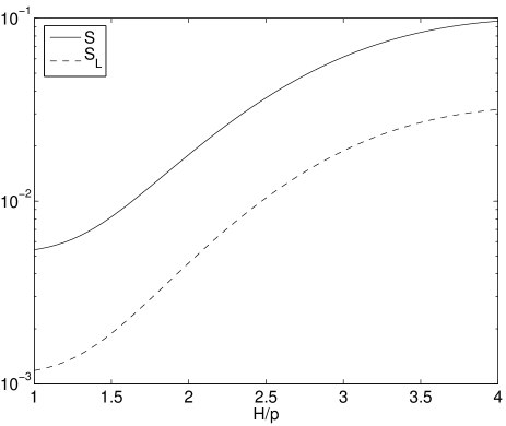
Figure 7.1: The evolution of entanglement entropy, $S$, and linear entropy, $S_{L}=|1-{\rm Tr}(\rho^{2})|$, as the mode stretches past the horizon for $\alpha=0.2$. This demonstrates that the non-linearities in the inflaton potential are capable of producing entanglement entropy between the coupled modes. Also note that $S$ scales monotonically with $S_{L}$.

The linear entropy, $S_{L}=1-\rm{Tr}(\rho^{2})$, is often used as a stand-in for the entanglement entropy since it can be computed more easily and in our case contains the same qualitative information,

$${\rm Tr}(\rho^{2})=\sum_{i=1}^{\infty}\sum_{j=1}^{i}\begin{cases}2|\rho_{ij}|^{2}&\text{if $j\neq i$,}\\ |\rho_{ij}|^{2}&\text{if $j=i$.}\end{cases}$$ (7.35)

A system with a finite Hilbert space spanned by $N$ basis states will have a maximum linear entropy $S_{L,{\rm max}}=(N-1)/N$.

From figure 7.1, we can see that this quantity is nearly proportional to the entropy. We will present the results both in terms of entanglement entropy and $S_{L}$.

Thermal Entropy and Classicality

The amount of entropy generated can be compared to the entropy of a thermal system that contains the same average number of particles. For a thermal system, the entropy is

$$S_{\rm th}=-\sum_{n=1}^{\infty}\rho_{n,{\rm th}}\ln\rho_{n,{\rm th}}$$ (7.36)

where the thermal density matrix is given by

$$\rho_{n,{\rm th}}=\frac{e^{-\beta E_{n}}}{\sum_{n^{\prime}=1}^{\infty}e^{-\beta E_{n^{\prime}}}}$$ (7.37)

and $n^{\prime}$ labels the Fock states. Since the energy is $m=n^{+}+n^{-}$, each $n^{\prime}$ state is $m+1$ times degenerate, the partition function can be written

$$\sum_{n^{\prime}=1}^{\infty}e^{-\beta E_{n^{\prime}}}=\sum_{m=0}^{\infty}(m+1)e^{-\beta m}=\frac{1}{(e^{-\beta}-1)^{2}}.$$ (7.38)

Using the relation

$$\langle n\rangle=\sum_{n^{\prime}=0}^{\infty}n\rho_{n^{\prime},\rm{th}}=\sum_{n=0}^{\infty}n(n+1)e^{-\beta n}(1-e^{-\beta})^{2}$$ (7.39)

we can eliminate $\beta$ for $\langle n\rangle$ using

$$e^{-\beta}=\frac{\langle n\rangle}{2+\langle n\rangle}$$ (7.40)

where $\langle n\rangle$ is the average number of particles in the reduced system. Finally, we can write the thermal entropy as

$$S_{\rm th}(\langle n\rangle)=-\sum_{m=0}^{\infty}(m+1)\frac{4\langle n\rangle^{m}}{(2+\langle n\rangle)^{m+2}}\ln\left(\frac{4\langle n\rangle^{m}}{(2+\langle n\rangle)^{m+2}}\right).$$ (7.41)

This quantity allows us to compare the entropy generated due to the coupling with the total energy of a thermal system at the same temperature. For example, if the information content of a system is defined as $I=S_{\rm th}-S$ then the relative information lost from the system due to the non-linear coupling term is

$$I_{\rm lost}=1-\frac{I}{I_{\rm max}}=\frac{S}{S_{\rm th}}.$$ (7.42)

Figure 7.2 shows that the rate of information loss due to the coupling is roughly the same as the rate of particle production.

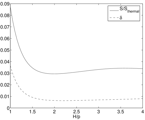
Figure 7.2: The fraction of information lost due to tracing out the unobserved degrees of freedom, defined by equation (7.42), and the separability parameter $\delta$ (equation 7.43) as the observed mode stretches past the horizon for $\alpha=0.2$. By the end of the simulation, $I_{\rm lost}$ appears to have leveled off to a constant few percent. For a separable (classical) system, we would expect $I_{lost}$ to grow to at least 0.5 to the right of the graph. If the system were to become classical, we would expect $\delta$ to grow to $1$. However, it too levels off to less than a percent.

Another approach for determining the classicality of a quantum system is to determine the conditions under which the subsystems can be considered separable states. Campo and Parentani argue that for Gaussian states at the threshold of separability and for $\langle n\rangle\gg 1$, the entanglement entropy between modes will be one half the entropy of the thermal state [26]. Since our states are not Gaussian, there is no known general separability condition. However, from the lack of growth in the information loss function shown in Figure 7.2, we can see that the Gaussian separability condition is unlikely to occur as $\langle n\rangle$ grows much larger than $1$ at times greater than can be shown on the figure. Therefore, these types of non-linear interactions alone are likely insufficient to cause the system to appear classical.

Another measure of separability used by Campo and Parentani is the parameter $\delta$ defined by the equation

$$|c|^{2}=n(n+1-\delta),$$ (7.43)

where $n={\rm Tr}(\rho a_{{\bf k}}^{\dagger}a_{{\bf k}})=\langle n^{+}\rangle$ and $c={\rm Tr}(\rho a_{{\bf k}}a_{{\bf-k}})$. The parameter, $\delta$, is a measure of the correlations between the ${\bf k}$ and $-{\bf k}$ modes. For Gaussian density matrices, it can be shown that separability occurs when $\delta=1$. The value of $\delta$ measured for our model is shown alongside the information loss function in Figure 7.2. In both cases, the measures flatten out after the modes leave the horizon and fail to grow as one would need for non-linearities to explain the classicality of the quantum state. We can generalize the definition of $c$ to measure the correlation between modes of different magnitudes of momenta in our system

$$d\equiv{\rm Tr}(\rho a_{{\bf-2k}}a_{{\bf k}}a_{{\bf k}}).$$ (7.44)

Although the interpretation of this quantity or $\delta$ is not as clear cut as for Gaussian density matrices, we find that both are useful and convenient tracers of the entanglement entropy.

Estimating the Sizes of $\lambda$ and $x_{\rm final}$

In order to match our above analysis with reality, we would like to make order of magnitude estimates for the parameters $\alpha$ in equation (7.18) and the final value of the $x$ at the end of inflation, $x_{\rm final}$.

For fluctuations in a scalar field other than the inflaton, the value of $\lambda$ is essentially arbitrary; however, the gravitational self-interaction of the field provides a strict lower bound. Burgess, et al. [22] give an estimate of this self-interaction,

$$\lambda_{g} \approx \frac{48}{(2\epsilon)^{3/2}}\left(\frac{H}{M_{\rm Pl}}\right)^{2}=\frac{128\pi}{(2\epsilon)^{3/2}}\left(\frac{M}{M_{\rm Pl}}\right)^{4}$$ (7.45)

$$\approx 6\times 10^{-16}\left(\frac{\epsilon}{0.01}\right)^{-3/2}\left(\frac{M}{10^{14}{\rm GeV}}\right)^{4},$$ (7.46)

where $M^{4}$ is the vacuum energy associated with the scalar field, and $\epsilon=\frac{M_{\rm Pl}^{2}}{2}\left(\frac{V^{\prime}}{V}\right)^{2}$ is a slow-roll parameter which may be larger than $1$ if the scalar field is not the inflaton. We have included a possible matter-dominated period following the end of inflation from scale factor $a_{\rm EI}$ to $a_{\rm RH}$ before reheating and taken $a$ to be the value of scale factor at the end of inflation.

The parameter $\alpha$ was introduced in equation (7.18) to replace

$$\alpha=\frac{\lambda VH}{8\sqrt{2\pi kM_{\rm Pl}}}.$$ (7.47)

So, if we take, for example, a mode of size $\omega=ck\sim 0.1{\rm Hz}=5\times 10^{-45}M_{\rm Pl}$ today, we arrive at an estimate for $\alpha$ due to gravitational self-interactions.

$$\alpha_{g}\approx 2\times 10^{-3}\left(\frac{\epsilon}{0.01}\right)^{-3/2}\left(\frac{M}{10^{14}{\rm GeV}}\right)^{6}\left(\frac{\omega}{0.1~{}{\rm Hz}}\right)^{-1/2}.$$ (7.48)

If the scalar field in question is the inflaton field, the gravitational self-interaction will dominate over self-coupling interactions.

The analysis here has assumed that reheating is quick and efficient [104, 205], but in principle the end of inflaton may be followed by a period of matter domination from scale factor $a_{\rm EI}$ to $a_{\rm RH}$ before reheating. With this generalization, the comoving Hubble rate at the end of inflation is

$$a_{\rm EI}H = \left(\frac{\pi^{2}}{30}g_{r}\frac{a_{\rm EI}}{a_{\rm RH}}\right)^{1/4}\left(\frac{8\pi}{3}\right)^{1/2}\frac{T_{0}M}{M_{\rm Pl}}$$ (7.49)

$$= 6.3\left(g_{r}\frac{a_{\rm EI}}{a_{\rm RH}}\right)^{1/4}\frac{M}{10^{14}{\rm GeV}}{\rm MHz},$$ (7.50)

where $M^{4}$ is the vacuum energy associated with the inflaton field, ($\approx\lambda M_{\rm Pl}^{4}/4$) and $g_{r}$ is the number of relativistic degrees of freedom at the end of reheating where the photon counts as two. The value of $x_{\rm final}$ (at the end of inflation) for the comoving scale $a_{\rm EI}H$ is simply unity and for other scales we have

$$x_{\hbox{\rm\scriptsize final}}=\frac{a_{\rm EI}H}{\omega}=6.3\times 10^{7}g_{r}^{1/4}\frac{M}{10^{14}{\rm GeV}}\frac{0.1~{}{\hbox{\rm Hz}}}{\omega}.$$ (7.51)

Consequently although the correlations are present on all scales, they are most obvious on the comoving scale of the Hubble length at the end of inflation (i.e. really small scales). On these small scales the density fluctuations are well into the non-linear regime today, but tensor fluctuations, gravitational waves (GW), would still be a loyal tracer of these correlations. Inflationary tensor perturbations were first calculated in  [181].

The expression given in equation (7.51) is very uncertain. Typically today’s Hubble scale is assumed to pass out through the Hubble length during inflation after about 50$-$60 $e-$foldings [116]; equation (7.51) gives 56 $e-$foldings before the end, so the centihertz scale would pass through the Hubble length 12$-$22 $e-$foldings before the end of inflaton. However, the former number is highly uncertain. For example, if inflation occurs at a lower energy scale or if there is a epoch of late “thermal inflaton” [128, 37, 38], the number of $e-$foldings for today’s Hubble scale could be as low as 25 [116], yielding $x_{\hbox{\rm\scriptsize final}}\ll\ 1$ for $ck\sim 0.1$ Hz.

Because the simulation increases in complexity as particles are produced (see figure 7.3), we are confined to keeping $x_{\rm final}\sim O(1)$. So, even though $\alpha$ may be small in reality, there may be sufficient time during inflation for even a small non-linearity to produce a great deal of entanglement entropy because of very large values of $x_{final}$.

Results

We would like to investigate how the amount of entropy generated in a single mode scales with the coupling strength and the duration of inflation (i.e. $\alpha$ and $x_{\rm final}$). Figure 7.1 explicitly shows the creation of entanglement entropy for $\alpha=1$ as the universe undergoes its inflationary phase. The horizontal axis, $x=H/p$, is the physical size of a mode with respect to the horizon scale. The entanglement entropy increases less quickly than exponentially, which would be a straight line on the figure. Unfortunately, as was mentioned previously, the computational size of the problem prevents us from simulating far past horizon crossing because the number of particles becomes too large. Figure 7.3 shows how many Fock states are in the reduced system at each time step in the simulation. The number of states being integrated is this number to the $3/2$ power, and the number of entries in the density matrix is the square of this number.

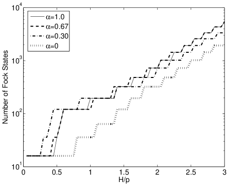
Figure 7.3: The number of Fock states associated with the reduced system.

The evolution of particles in the system is shown in figure 7.4. Our results are consistent with those found in Heyl [82] and show a nearly exponential evolution of the average particle number. Moreover, we can look at the evolution of each mode separately. For $\lambda=0$, each mode evolves according to the same equations of motion, and in this case, there is no difference between the rate that each of the modes evolves. However, the nature of the interaction between the modes is not symmetric because the decay of a single $M$ mode particle results in 2 $N$ mode particles and therefore the interaction results in an increased rate of production of $N$ mode particles, relative to the $M$ mode. Figure 7.5 shows how the entanglement entropy scales with average particle number when $\alpha=0.2$.

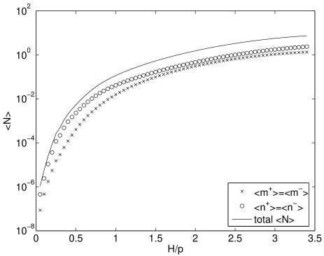
Figure 7.4: Evolution of the average particle numbers for each mode for $\alpha=1.0$

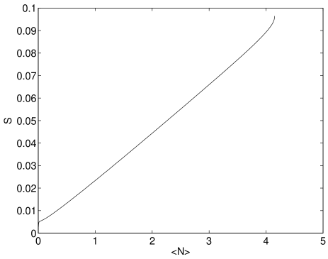
Figure 7.5: Entanglement entropy vs. average particle number for $\alpha=0.2$

We performed the simulation for a variety of values for the coupling, $\alpha$, spanning several orders of magnitude. Figure 7.6 shows entropy generation as a function of $\alpha$ for a variety of inflation durations $x_{\rm final}$. From this plot, we can see that $S_{\rm final}$ scales roughly as a power law in $\alpha$. Most of the $\alpha$ dependence can be removed by dividing $S_{\rm final}$ by $\alpha^{1.75}$. Doing this also helps to illustrate how $S_{\rm final}$ scales with $x_{\rm final}$. As expected, there is no entropy generated without the coupling terms (i.e. when $\alpha=0$). In this case, there is no communication between modes of the scalar field and they evolve independently.

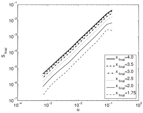
Figure 7.6: von Neumann entropy vs. $\alpha$ for various values of $x_{\rm final}$

As was mentioned earlier, $S_{L}$ is a useful stand-in for $S$ that can be computed faster than $S$. Figure 7.7 echoes the previous results in terms of $S_{L}$ instead of $S$. In this case, $1-\rm{Tr}(\rho^{2})$ scales more like $\alpha^{2}$ instead of $\alpha^{1.75}$. However, both $S_{L}$ and $S$ demonstrate the same qualitative behaviour.

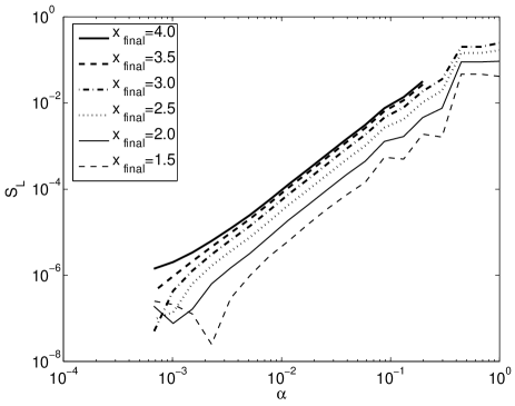
Figure 7.7: $S_{L}$ vs. $\alpha$ for various values of $x_{\rm final}$

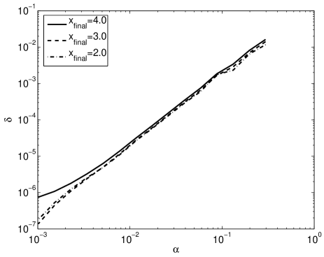
Figure 7.8: $\delta$, defined in equation (7.43) scales with $\alpha$ in much the same way as $S_{L}$, but is less costly to compute.

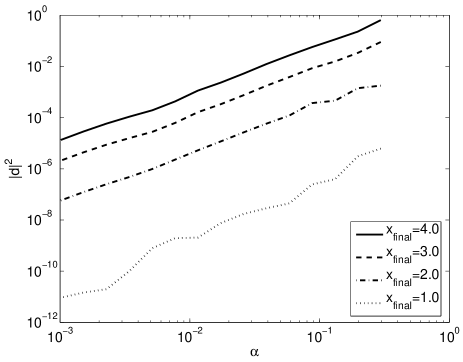
Figure 7.9: $|d|^{2}=|{\rm Tr}(\rho a_{{\bf 2k}}a_{{\bf k}}a_{{\bf k}})|^{2}$ scales with $\alpha$ in much the same way as $S$, but is less costly to compute.

In addition, we have found other useful stand-ins for the entanglement entropy that are easier to compute and scale similarly with $\alpha$. The $\delta$ parameter, defined in (7.43), scales roughly like an $\alpha^{2}$ power law much like $S_{L}$. Figure 7.8 shows the power law behaviour of this function. Additionally, if we use a simple measure of correlation between entangled modes, $|d|^{2}$ (equation 7.44), we find that its scales like $\alpha^{1.85}$ (see figure 7.9), and so can be a useful stand-in for the von Neumann entropy, $S\propto\alpha^{1.75}$.

In the real universe, we are dealing with small values of $\lambda$ (and therefore of $\alpha$) and very large values of $x$. However, the simulation outlined in this chapter is limited because its computational complexity increases dramatically as particles are produced, even for small values of the coupling, $\alpha$. Moreover, for small values of $\alpha$, the production of entropy is too small to be meaningful. While the dependence of $S$ on $\alpha$ nearly follows a power law, there is no simple relation describing the dependence of $S$ on $x_{\rm final}$. The value $S_{L}$ is approximately proportional to $\alpha^{2}x_{\rm final}^{3}$ over a wide range of $\alpha$ and the modest range $x$ probed by the simulations; therefore, very roughly, we can write the scaling law as $S_{L}\propto\alpha^{2}x_{\rm final}^{3}$ where

$$S_{L}\approx 10^{16}g_{r}^{3/4}\left(\frac{M}{10^{14}{\rm GeV}}\right)^{15}\left(\frac{\omega}{0.1~{}{\rm Hz}}\right)^{-4}.$$ (7.52)

Of course, only values of $S_{L}$ less than unity make sense, so a larger value from the fitting formula indicates that $S_{L}$ is very close to one. However, a value of $S_{L}<1$ is obtained by lowering the mass scale of inflation below

$$M<8\times 10^{12}\left(\frac{\omega}{0.1~{}{\rm Hz}}\right)^{-4/15}{\rm GeV};$$ (7.53)

therefore, if the energy scale of inflation is low, the quantum states of fluctuations at $\omega\sim 0.1$ Hz will remain coherent despite the non-linear coupling.

The simulation was checked for consistency in several ways. First, we traced the probability throughout the simulation measured both by the sum of squares of the matrix elements $\sum_{m^{\pm},n^{\pm}=0}^{\infty}A_{m^{\pm},n^{\pm}}$ and the trace of the density operator. Both of these quantities were conserved to a few parts in $10^{-7}$. Moreover, we estimated the level of numerical error by rerunning the simulation with a variety of phase rotations multiplying the initial wavefunction. The standard deviation of the results from these numerical changes in the initial conditions give us an idea of the level of numerical error in the simulation, which were typically at the level of one part per thousand.

Conclusions

In this chapter we have developed a model in which two modes of a scalar field evolve during inflation and we have computed the entanglement entropy between them. The entanglement entropy generated between observed and unobserved modes in the inflaton field give the appearance that entropy is being produced, even though the scalar field remains in an overall pure state. The preceding results clearly show that non-linearities in the inflaton potential give rise to a generation of entanglement entropy between observed modes and unobserved modes in a scalar field during inflation. This entropy is an additional source to that caused by coupling to external degrees of freedom [101], entanglement between the inside and outside of the horizon [172] and that which is created during reheating after inflation has ended.

We have attempted to extrapolate the results of our simulation to the real universe. The relevant parameters determining the amount of entropy generated via non-linearities are the strength of the coupling $\alpha_{g}\sim 10^{-3}$ and the scale of the fluctuation at the end of inflation given by the dimensionless parameter $x_{\rm final}\sim 10^{7}$. The entanglement entropy was found to scale like $\alpha^{1.75}$ for a fixed $x_{\rm final}$. The dependence of $S_{L}$ on $x_{\rm final}$ for a given value of $\alpha$ is not as straightforward, but $S_{L}\propto x_{\rm final}^{3}$ over a short range of $x_{\rm final}$ values. Based on these rough scaling patterns, we estimate that non-linearities due to gravity and inflaton self-coupling are insufficient to decohere modes that spend only a few Hubble times at super-horizon scales. In particular, if the energy scale of inflaton is less than $10^{13}$ GeV, fluctuations at about 0.1 Hz may remain coherent.

We found two measures of the decoherence related to the correlations between modes of different momenta provide a faithful estimate of the entanglement entropy in our model — one of these measures is new to this work ($d$) and specifically probes the non-linear coupling between modes. In particular these estimates are very inexpensive to calculate as compared to the von Neumann entropy and should prove useful for more detailed models of entropy generation.

It is usually assumed that the main contribution to the entropy observed in the density perturbations is generated during reheating, when the inflaton decays. However, the analysis demonstrates that entropy can be generated independently of reheating, provided there is even a small non-linearity in the scalar potential; therefore, the results are applicable to scalar fields that do not participate in reheating. For example, the gravitational wave background can be treated as a pair of scalar fields, so even tensor fluctuations may contribute to the entropy and the classicality of the distribution of density perturbations in this way and observations of the gravitational wave background at high frequency could reveal the quantum mechanical origin of density fluctuations.

Part II Electromagnetic Waves Near Magnetars

Chapter 8 The Magnetized Vacuum

In magnetic fields near or above the critical field strength, $B_{k}=4.4\times 10^{13}$ Gauss, the Larmor radius of the electron becomes comparable to its Compton wavelength. In this regime, the vacuum fluctuations of $\mathrm{QED}$ interact significantly with the background magnetic field, altering the physical properties of the vacuum. We may take these effects into account by defining a new classical theory with a Lagrangian that effectively accounts for the quantum fluctuations by averaging over them. The resulting theory describes the quantum vacuum with a strong background field as a nonlinear optical medium. In this chapter, I review the history and theory behind this idea.

The purpose of this chapter is to introduce the interesting physics behind magnetic fields near to and exceeding a critical value determined by the electron mass and electric charge, $B_{k}=\frac{m^{2}}{e}=4.4\times 10^{13}$ Gauss. Magnetic fields have important physical effects even at the scale of Earth’s weak magnetic field, which is typically less than one Gauss. Here on Earth, the magnetic field is strong enough to magnetize ferromagnetic materials. This effect is used for navigation in both human technologies and by some animals, for example [96]. Large fields used in research labs (for magnetic resonance imaging ($\mathrm{MRI}$), for example) are on the order of $10^{4}$ Gauss [201]. The quantum critical field is well beyond the strength of fields that we can achieve in labs. Fortunately, extreme magnetic fields in excess of the critical field strength are believed to exist around neutron stars. The emissions from these neutron stars are strongly influenced by their incredible magnetic fields.

Quantum effects can alter the structure of the vacuum when we include a background magnetic field near the quantum critical field strength. For example, in two-dimensional $\mathrm{QED}$₂₊₁, a classically stable uniform magnetic field is unstable to the formation of inhomogeneities when QED effects are taken into account [29]. This result motivates the question of whether $\mathrm{QED}$₃₊₁ also prefers more interesting structures over a strong, uniform magnetic field. If so, what might these structures look like?

Here, we wish to study these questions by looking at the effective classical theory that is obtained by averaging over quantum effects to the one-loop level. This picture results in an effective action of $\mathrm{QED}$ where the quantum effects appear as correction terms to the familiar classical Maxwell action. These correction terms destroy the linearity of Maxwell’s equations, and allow light waves to interact with one another. So, the quantum vacuum in the presence of a strong electromagnetic field behaves like a non-linear optical medium that may be capable of supporting novel electromagnetic structures like solitons.

Solitons are local wave excitations that can travel undisturbed for considerable distances. They commonly appear in a wide variety of wave equations displaying nonlinear and dispersive behavior. Electromagnetic solitons are known to exist in certain nonlinear optical materials where they are called light bullets [187]. It is therefore possible that solitons can be found in the systems similar to the magnetar magnetosphere model described above, where there is a strong magnetic background field and a plasma. Recently, perturbative methods revealed electromagnetic waves in a magnetized plasma with slowly varying soliton solutions [109, 31].

Strong-Field $\mathrm{QED}$

Research into the interactions between the electronic vacuum and external electromagnetic fields predates modern $\mathrm{QFT}$ and was among the earliest applications of $\mathrm{QED}$. In 1936, Heisenberg and Euler [79] and Weisskopf [200] independently derived the effective action due to electronic fluctuations from electron-hole theory. In 1951, Schwinger re-derived the result from the new theory of $\mathrm{QED}$ [168]. The 1960s and early 1970s saw considerable progress in understanding the one-loop corrections to the classical action in $\mathrm{QED}$ [102, 45, 2, 140, 68].

$\mathrm{QED}$ is the quantum field theory describing the interactions between electrons (and positrons) and light. The electrons are described by a Dirac spinor field, $\psi(x)$, and the photon field is the vector field, $A_{\mu}(x)$. In each case, the quantized fluctuations of the field are identified with the corresponding particles. The Lagrangian is [199, 157, 68]

$${\cal L}=\bar{\psi}(i\not{\partial}+e\not{A}-m)\psi-\frac{1}{4}F_{\mu\nu}F^{\mu\nu}.$$ (8.1)

The Feynman slash indicates a vector-index contraction with the Dirac gamma matrices, $\not{A}\equiv\gamma^{\mu}A_{\mu}$ and $\bar{\psi}$ is defined by $\bar{\psi}\equiv\psi^{\dagger}\gamma^{0}$. We may incorporate the effects of a classical background electromagnetic field, $\tilde{A}_{\mu}^{0}({\bf q})$, through a new interaction with the Feynman rule

$$-ie\gamma^{\mu}\tilde{A}_{\mu}^{0}({\bf q}).$$ (8.2)

This interaction dresses all of the fermion propagators, including internal lines.

The background field may be thought of as an average over all possible quantum fluctuations of a quantum field composed of a large number of photons. For weak background fields, the new interaction may be treated perturbatively. However, when the fields exceed $\frac{1}{2}\frac{m^{2}}{e}\approx 2\times 10^{13}\mbox{G}$, the perturbation series fails to converge.

Neutron Stars and Extreme Magnetism

The extreme strengths of the quantum critical fields make effects from the quantum vacuum difficult to probe in terrestrial experiments. Very large magnetic fields up to $10^{19}$G can be created in heavy ion collisions [161, 175]. Unfortunately, experimental access to these fields is limited since they only exist in microscopic volumes. In general, the largest macroscopic, continuous magnetic fields that can be created in the lab are on the order of tens of Teslas, or tens of thousands of Gauss  [156]. Pulsed magnetic fields of several kiloteslas can be produced with the use of explosives [17]. However, these fields are less than a millionth the strength of the $\mathrm{QED}$ critical field (see figure 8.1). Luckily, nature occasionally provides us with very strong astrophysical magnets.

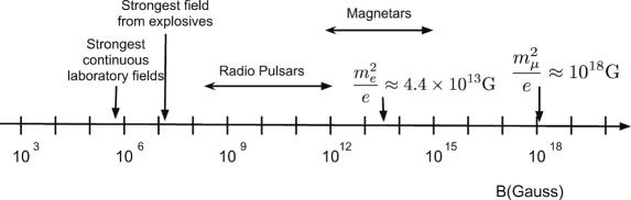
Figure 8.1: Orders of magnitudes of magnetic fields in terrestrial experiments and astrophysical objects.

A few times per century in our galaxy, a massive star will reach the end of its nuclear fuel supply and will no longer have sufficient thermal pressure to support itself against gravitational collapse. The energy from the collapse may blow away the outer layers of the star in a supernova explosion, leaving behind an ultradense core. In most of these supernova explosions, the remaining core becomes a neutron star, supported from further collapse by the degeneracy pressure of its nucleons, and often with an intense magnetic field, approaching or exceeding the quantum critical field. Therefore, our galaxy provides us with real astrophysical laboratories for exploring the physics of the magnetized vacuum.

The idea of a neutron star was first proposed by Landau in 1932 [112], and in 1934, Baade and Zwicky suggested that one could result from the supernovae of a star with a massive iron core exceeding the Chandrasekhar mass [9]. In this case, the gravitational pressure of the collapsing core would exceed the electron degeneracy pressure, causing a collapse to incredible densities until the neucleon degeneracy pressure eventually stabilized the star.

In 1968, Bell and Hewish observed an unusual steadily-pulsing astrophysical radio signal, marking the discovery of a new class of stars called ‘pulsars’ [80]. Pulsars were quickly identified as strongly magnetized neutron stars by Pacini [152] and Gold [62]. Soon afterwards, this link was solidified with strong observational evidence when a pulsar was discovered near the Crab Nebula [179]. The radio pulsations from the new class of stars were explained by relativistic plasma velocities in the magnetosphere leading to charged particles emitting acceleration radiation beamed along the magnetic axis. When the magnetic axis and the rotation axis are misaligned, the result is a lighthouse beacon of radio emission consistent with the observations. To date, more than 2000 pulsars have been identified [129] (see figure 8.2).

The incredible surface magnetic field strengths of neutron stars arises partly because the magnetic flux flowing through the surface of the progenitor star becomes frozen in the core as it collapses. The mass-radius ($m-R$) relation for a neutron star supported by non-relativistic degeneracy pressure is

$$R\approx 4.5\frac{\hbar^{2}}{Gm_{p}^{8/3}}M^{-1/3}.$$ (8.3)

Putting the canonical neutron star mass of $M\approx 1.4M_{\odot}$  [193] into this expression yields an expected radius of $R\sim 1.2\times 10^{4}\mbox{m}$, roughly the size of a city. During the collapse to this astronomically tiny radius, the star is strongly ionized with free electrons and protons and is nearly a perfect conductor. The magnetic field lines are frozen in the star. The constant flux condition requires

$$\Phi=\int{\bf B}\cdot d{\bf A}\sim{\bf B}\cdot{\bf A}={\rm constant.}$$ (8.4)

So, when the radius shrinks from a typical solar radius of $10^{9}$m to $10^{4}$m, the magnetic field strength at the surface is amplified by 10 orders of magnitude. Through this effect alone, neutron stars are expected to have magnetic fields of $10^{12}-10^{13}$ Gauss.

The magnetic fields of astrophysical neutron stars can be inferred from observations of pulsars. The most common way of doing this is by equating the observed spin-down power with magnetic dipole radiation [133]. For example, consider a crude model in which the pulsar is a rigidly rotating sphere with a dipole magnetic field. For a pulsar with mass $M$, radius $R$, period $P$, and period derivative, $\dot{P}$, we have

$$\dot{E}_{{\rm spin-down}}=-\frac{8}{5}\pi^{2}MR^{2}\frac{\dot{P}}{P^{3}}.$$ (8.5)

This spin-down energy loss is a consequence of the energy radiated away as dipole radiation,

$$\dot{E}_{{\rm dipole}}=-\frac{8\pi^{4}}{3c^{3}}\frac{B_{0}^{2}R^{6}}{P^{4}}.$$ (8.6)

Equating these expressions gives an expression for the surface magnetic field in terms of $P$ and $\dot{P}$

$$B_{0}=\left(1.3\times 10^{19}~{}\frac{\rm G}{\sqrt{\rm s}}\right)\sqrt{P\dot{P}}.$$ (8.7)

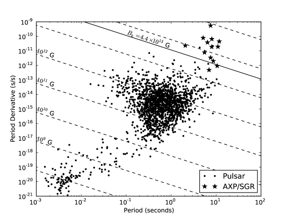
Figure 8.2: The $P$-$\dot{P}$ diagram for the $\sim$1800 known pulsars. The magnetars (anomalous X-ray pulsars and soft gamma repeaters) occupy the top right region of the diagram and are labelled with stars. The magnetic fields indicated by equation (8.7) are shown with diagonal dotted lines, and the line representing the critical field is shown as a solid line. This data was collected from the ATNF Pulsar Catalogue[69, 129]

.

The magnetic fields inferred from these measurements are largely consistent with the estimate we made above (see figure 8.2). However, there are two related classes of pulsars which appear to have even larger magnetic fields. These are $\mathrm{AXP}$s and $\mathrm{SGR}$s, the so-called magnetars. These pulsars generally have periods and period derivatives which imply magnetic fields in the range $10^{14}-10^{16}$ Gauss.

A favoured explanation for such intense fields is that they are generated by a convective dynamo mechanism in the first few seconds of the proto-neutron star’s life [189]. The neutron star fluid is a very good conductor as it contains free protons and electrons. If the star is born rotating very quickly, and is differentially rotating, the magnetic field lines can be dragged through the conductive neutron star fluid in convection currents. The magnetic field is built up through this dragging process. This is similar to the dynamo mechanisms which generate magnetic fields in the Earth and Sun. However, if it works efficiently in newborn neutron-stars, it can generate magnetic fields of up to $10^{16}$ Gauss [189].

The inferred magnetic field strengths can also be checked for consistency against other lines of observational evidence (for a review, see [202, 76]). In the cases of some pulsars, spectral features can be seen which imply large magnetic fields ($10^{13}-10^{15}~{}{\rm G}$) if they are interpreted as proton cyclotron resonances. For a few X-Ray pulsars, electron cyclotron spectral features have been detected implying magnetic fields up to $10^{13}$ G. There are strong theoretical arguments that the emissions from $\mathrm{SGR}$s and $\mathrm{AXP}$s are likely powered by fields exceeding the quantum critical field [190, 191]. Similarly, the giant flares and bursts from $\mathrm{SGR}$s have been argued to be consistent with highly-magnetized stars [192, 202]

The McGill $\mathrm{AXP}$/$\mathrm{SGR}$ catalog [70] lists 23 confirmed or candidate magnetars at the time of writing: 11 $\mathrm{SGR}$s (7 confirmed, 4 candidates), and 12 $\mathrm{AXP}$s (9 confirmed, 3 candidates). A thorough, recent review of the physics of highly magnetized neutron stars can be found in [76].

The $\mathrm{QED}$ Effective Action

The effective action can be viewed as a quantum-corrected expression of the classical action which averages over all possible quantum fluctuations of the field. Thus, it provides a means of interpolating between the classical and quantum regimes. The quantum correction terms destroy the linearity of Maxwell’s equations, so the quantum vacuum state in the presence of external fields resembles a non-linear optical medium which can be polarized and magnetized. In this section, we will derive the effective action of $\mathrm{QED}$.

Consider a function, $E[J^{\mu},\bar{\eta},\eta]$, representing the energy of the vacuum as a function of external sources, $J^{\mu}$, $\bar{\eta}$, and $\eta$. The sources $\bar{\eta}$ and $\eta$ are anti-commuting (Grassman) variables. We may use this functional to express a partition functional:

$$Z[J^{\mu},\bar{\eta},\eta] = e^{-iE[J^{\mu},\bar{\eta},\eta]/\hbar}$$ (8.8)

$$= \int\mathcal{D}A_{\mu}\mathcal{D}\psi\mathcal{D}\bar{\psi}\exp\left(\frac{i}{\hbar}\int d^{4}x(\mathcal{L}+J^{\mu}A_{\mu}+\bar{\eta}\psi+\bar{\psi}\eta)\right).~{}~{}~{}$$ (8.9)

There is a strong analogy with statistical mechanics. Here, the energy functional is the analog of the Helmholtz free energy. We would like to define the effective action, $\Gamma[A_{\mu}^{0}]$, so that stable quantum states of the theory are solutions to

$$\frac{\delta\Gamma[A_{\mu}^{0}]}{\delta A_{\mu}^{0}(x)}\biggr{|}_{J^{\mu}=0}=0$$ (8.10)

where $A_{\mu}^{0}(x)=\langle 0|A_{\mu}(x)|0\rangle$ is a weighted average of the field configuration over all possible quantum fluctuations. We refer to this field as a classical field.

This problem is analogous to finding the most probable thermodynamic state in a thermally fluctuating background. This state is a minimum of the Gibbs free energy, $G$, which is related to the Helmholtz free energy, $F$, by a Legendre transformation

$$G=F-V\frac{\partial F}{\partial V}\biggr{|}_{T}=F+PV.$$ (8.11)

Analogously, the effective action is defined in terms of a Legendre transformation of the energy functional

$$\Gamma[A_{\mu}^{0},\bar{\psi}^{0},\psi^{0}]=-E[J^{\mu},\bar{\eta},\eta]-\int d^{4}y(J^{\mu}(y)A_{\mu}^{0}(y)+\bar{\eta}(y)\psi^{0}(y)+\bar{\psi}^{0}(y)\eta(y)).$$ (8.12)

We compute the energy functional by expanding the fields about their classical values (i.e. $A_{\mu}(x)=A_{\mu}^{0}(x)+\Delta A_{\mu}(x)$):

$$E[J_{\mu},\bar{\eta},\eta] = \int d^{4}x\left({\cal L}[A_{\mu},\bar{\psi},\psi]+J^{\mu}A_{\mu}+\bar{\eta}\psi+\bar{\psi}\eta\right)$$ (8.14)

$$= \int d^{4}x\left({\cal L}[A_{\mu}^{0},\bar{\psi}^{0},\psi^{0}]+J^{\mu}A^{0}_{\mu}+\bar{\eta}\psi^{0}+\bar{\psi}^{0}\eta\right)$$

$$+\int d^{4}x\biggr{[}\Delta A_{\mu}(x)\left(\frac{\delta{\cal L}}{\delta A_{\mu}(x)}+J^{\mu}\right)$$

$$+\left(\frac{\delta{\cal L}}{\delta\psi(x)}+\bar{\eta}\right)\Delta\psi(x)+\Delta\bar{\psi}(x)\left(\frac{\delta{\cal L}}{\delta\bar{\psi}(x)}+\eta\right)\biggr{]}$$

$$+\frac{1}{2}\int d^{4}xd^{4}y\biggr{[}\Delta A_{\mu}(x)\Delta A_{\nu}(y)\frac{\delta^{2}{\cal L}}{\delta A_{\mu}(x)\delta A_{\nu}(y)}$$

$$+\Delta\bar{\psi}(x)\frac{\delta^{2}{\cal L}}{\delta\bar{\psi}(x)\delta\psi(y)}\Delta\psi(y)+\Delta A_{\mu}(x)\frac{\delta^{2}{\cal L}}{\delta A_{\mu}(x)\delta\psi(x)}\Delta\psi(x)$$

$$+\Delta\bar{\psi}(x)\frac{\delta^{2}{\cal L}}{\delta\bar{\psi}(x)\delta A_{\mu}(x)}\Delta A_{\mu}(x)\biggr{]}+...$$

In order to have an effective action which is independent of the external currents, we must find a relationship between the currents and the classical fields. Here we will promote the result from lowest order perturbation theory to a requirement connecting the currents $J^{\mu}$, $\eta$, and $\bar{\eta}$ to the classical fields $A_{\mu}$, $\bar{\psi}$ and $\psi$. That is, the fields and currents must obey the classical field equations. For example,

$$\frac{\delta{\cal L}}{\delta A_{\mu}}\biggr{|}_{A_{\mu}=A_{\mu}^{0}}+J_{\mu}=\bar{\psi}e\gamma^{\mu}\psi+J^{\mu}-\partial_{\nu}F^{\nu\mu}=0.$$ (8.15)

We may imagine this step as replacing the currents in the energy functional with whatever currents are required to satisfy (8.15) exactly, with the relationship between the two currents being determined order-by-order in perturbation theory. In this case, the first-order derivative terms vanish. If we terminate the series at the second-order derivative terms (the one-loop approximation), the energy functional is a Gaussian integral, which we can evaluate by treating the functional derivatives as infinite dimensional matrices in a field-configuration space:

$$E[J_{\mu},\bar{\eta},\eta] = \int d^{4}x\left({\cal L}^{0}+J^{\mu}A^{0}_{\mu}+\bar{\eta}\psi^{0}+\bar{\psi}^{0}\eta\right)$$ (8.17)

$$+i\hbar{\rm ln}\int\mathcal{D}A_{\mu}\mathcal{D}\psi\mathcal{D}\bar{\psi}\exp\frac{i}{2\hbar}\int d^{4}xd^{4}y\biggr{[}$$

$$\Delta A_{\mu}(x)\Delta A_{\nu}(y)\frac{\delta^{2}{\cal L}}{\delta A_{\mu}(x)\delta A_{\nu}(y)}$$

$$+\Delta\bar{\psi}(x)\frac{\delta^{2}{\cal L}}{\delta\bar{\psi}(x)\delta\psi(y)}\Delta\psi(y)\biggr{]}$$

$$= -\int d^{4}x\left(-\frac{1}{4}F^{0}_{\mu\nu}F^{0,\mu\nu}+J^{\mu}A_{\mu}^{0}\right)$$

$$-\frac{i\hbar}{2}{\rm ln~{}Det}\left[-\frac{\delta^{2}{\cal L}}{\delta A_{\mu}(x)\delta A_{\nu}(y)}\right]$$

$$+\frac{i\hbar}{2}{\rm ln~{}Det}\left[-\frac{\delta^{2}{\cal L}}{\delta\bar{\psi}(x)\delta\psi(y)}\right]+{\rm Constant~{}Terms}.$$

The different signs in front of the functional determinants in the above equation arise due to the difference between Gaussian integration involving Grassman versus standard complex variables:

$${\rm Grassman:}~{}\int d{\bf\eta}d{\bf\psi}\exp(-\eta_{\mu}^{*}\psi_{\nu}b^{\mu\nu})={\rm det}(b);$$ (8.18)

$${\rm Standard:}~{}\frac{1}{\pi}\int d{\bf\theta}d{\bf\phi}\exp(-\theta_{\mu}\phi_{\nu}b^{\mu\nu})=\frac{1}{{\rm det}(b)}.$$ (8.19)

The Legendre transformation, (8.12), eliminates the $J^{\mu}$ dependent terms and we are left with

$$\Gamma[A_{\mu}^{0}] = \int d^{4}x\left(-\frac{1}{4}F^{0}_{\mu\nu}F^{0,\mu\nu}\right)+\frac{i\hbar}{2}{\rm ln~{}Det}\left[-\frac{\delta^{2}{\cal L}}{\delta A_{\mu}(x)\delta A_{\nu}(y)}\right]$$ (8.20)

$$-\frac{i\hbar}{2}{\rm ln~{}Det}\left[-\frac{\delta^{2}{\cal L}}{\delta\bar{\psi}(x)\delta\psi(y)}\right]+{\rm Constant~{}Terms}.$$

The functional determinants in the above expression are divergent, so we must renormalize the expression. We therefore require that the effective action vanishes when the classical action vanishes. So, we subtract off two terms corresponding to the functional determinants evaluated at $A_{\mu}^{0}=0$. The term arising due to the photon field then vanishes at the one-loop order since the photon fluctuations do not interact with the background field except through the fermion loop. We are left with

$$\Gamma[A_{\mu}^{0}]=\int d^{4}x\left(-\frac{1}{4}F^{0}_{\mu\nu}F^{0,\mu\nu}\right)-i\hbar{\rm ln~{}Det}\left[\frac{\not{p}+e\not{A}^{0}-m}{\not{p}-m}\right].$$ (8.21)

We may put the one-loop effective action into a more manageable form by using the linear algebra result, ${\rm ln~{}Det}A={\rm Tr~{}ln}A$. Additionally, we may simplify the operator using invariance under the charge conjugation operator, $C(\not{p}+e\not{A}^{0})C^{-1}=-(\not{p}+e\not{A}^{0})^{T}$. Then,

$${\rm Tr~{}ln}\left[\frac{\not{p}+e\not{A}^{0}-m}{\not{p}-m}\right]={\rm Tr~{}ln}\left[\frac{\not{p}+e\not{A}^{0}+m}{\not{p}+m}\right]=\frac{1}{2}{\rm Tr~{}ln}\left[\frac{(\not{p}+e\not{A}^{0})^{2}-m^{2}}{\not{p}^{2}-m^{2}}\right],$$ (8.22)

where the final expression is half the sum of the first two expressions. The effective action is now in its most useful, fully general form:

$$\Gamma[A_{\mu}^{0}]=\int d^{4}x\left(-\frac{1}{4}F^{0}_{\mu\nu}F^{0,\mu\nu}\right)-i\hbar{\rm Tr~{}ln}\left[\frac{(\not{p}+e\not{A}^{0})^{2}-m^{2}}{\not{p}^{2}-m^{2}}\right].$$ (8.23)

Proper-Time Formalism

The proper-time formalism is a useful trick for regularizing the functional determinants in terms of a fictional proper-time parameter while preserving the gauge and Lorentz invariance of the expressions [48, 168]. We may express the logarithm appearing in the effective action in terms of an integral using the following identity:

$$\ln\frac{a}{b}=\int_{0}^{\infty}\frac{dT}{T}\left[\exp{(iT(b+i\epsilon))}-\exp{(iT(a+i\epsilon))}\right].$$ (8.24)

Employing this identity, we may write

$${\rm Tr~{}ln}\left[\frac{\not{p}+e\not{A}^{0}-m}{\not{p}-m}\right] = -\frac{1}{2}\int d^{4}x\int_{0}^{\infty}\frac{dT}{T}e^{-iTm^{2}}$$ (8.25)

$$\times{\rm tr}\biggr{(}\langle x|e^{iT(\not{p}+e\not{A}^{0})^{2}}|x\rangle-\langle x|e^{iT\not{p}^{2}}|x\rangle\biggr{)}$$

where previously ${\rm Tr}$ signified a trace over both spin and coordinate degrees of freedom, we use ${\rm tr}$ to signify that the trace is now only over spinorial components.

Beyond its function as a useful technical tool, the proper-time formalism also provides an intuitive picture of the functional determinants. The object $\langle x|e^{iT(\not{p}+e\not{A}^{0})^{2}}|x\rangle$ can be thought of as a transition amplitude in standard quantum mechanics for a fictitious particle with space-time coordinates evolving in proper-time, $T$, under the influence of a “Hamiltonian”, $-(\not{p}+e\not{A}^{0})^{2}$, that depends only on the $T$-independent electromagnetic field. Thus, we have expressed the functional determinant in terms of the motion of a “particle” that obeys a $T$-dependent Schrödinger-like equation in the given $T$-independent electromagnetic field.

Effective Lagrangian in a Uniform Field

The effective Lagrangian can only be evaluated analytically for a small number of field configurations. The homogeneous field case is the simplest of these. We begin by considering the Lorentz frame and coordinate system where the classical electric and magnetic fields are parallel and point in the $x^{3}$-direction. The magnitudes of the fields in this frame provide us with a set of Lorentz scalar field invariants, $a\equiv|{\bf E}|$ and $b\equiv|{\bf B}|$.

The operator of interest can be separated into a scalar and a fermion term,

$$-(\not{p}+e\not{A}^{0})^{2}=(p_{\mu}+eA^{0}_{\mu})^{2}-\frac{1}{2}e\sigma^{\mu\nu}F_{\mu\nu},$$ (8.26)

where $\sigma^{\mu\nu}=\frac{i}{2}[\gamma^{\mu},\gamma^{\nu}]$. This means that the trace factorizes.

First, consider the scalar factor,

$${\rm tr}\left(\langle x|e^{iT(p_{\mu}+eA^{0}_{\mu})^{2}}|x\rangle\right).$$ (8.27)

In this coordinate system and frame, we may choose a gauge so that $A^{3}=-ax^{0}$, and $A^{1}=-bx^{2}$. The relevant operator then expands as

$$(p_{\mu}+eA^{0}_{\mu})^{2} = p_{0}^{2}-p_{2}^{2}-(p_{1}+ebx_{2})^{2}-(p_{3}+eax_{0})^{2}$$ (8.29)

$$= {\rm exp}\left(-i\frac{p_{2}p_{1}}{eb}-i\frac{p_{0}p_{3}}{ea}\right)\left[p_{0}^{2}-p_{2}^{2}-(ebx_{2})^{2}-(eax_{0})^{2}\right]$$

$$\times{\rm exp}\left(i\frac{p_{2}p_{1}}{eb}+i\frac{p_{0}p_{3}}{ea}\right),$$

where we have used the shift operator, $e^{-ip_{1}c}f(x_{1})e^{ip_{1}c}=f(x_{1}+c)$. The scalar factor can then be evaluated by taking the trace in momentum space,

$${\rm tr}\left(\langle x|e^{iT(p_{\mu}+eA^{0}_{\mu})^{2}}|x\rangle\right) = \int\frac{dp_{3}dp_{1}}{(2\pi)^{4}}dp_{0}dp_{0}^{\prime}dp_{2}dp_{2}^{\prime}$$ (8.31)

$$\times{\rm exp}\left[i(p_{0}^{\prime}-p_{0})\left(x_{0}+\frac{p_{0}}{ea}\right)\right]$$

$$\times{\rm exp}\left[i(p_{2}^{\prime}-p_{2})\left(x_{2}+\frac{p_{2}}{eb}\right)\right]$$

$$\times\langle p_{0}|{\rm exp}[iT(p_{0}^{2}-e^{2}a^{2}x_{0}^{2})]|p_{0}^{\prime}\rangle$$

$$\times\langle p_{2}|{\rm exp}[iT(p_{2}^{2}+e^{2}b^{2}x_{2}^{2})]|p_{2}^{\prime}\rangle$$

$$= \frac{e^{2}ab}{(2\pi)^{2}}\int_{-\infty}^{\infty}dp_{0}\langle p_{0}|{\rm exp}[iT(p_{0}^{2}-e^{2}a^{2}x_{0}^{2})]|p_{0}^{\prime}\rangle$$

$$\times\int_{-\infty}^{\infty}dp_{2}\langle p_{2}|{\rm exp}[iT(p_{2}^{2}+e^{2}b^{2}x_{2}^{2})]|p_{2}^{\prime}\rangle.$$

The remaining traces can be evaluated by using the known eigenvalues of the harmonic oscillator. For example, we evaluate the second one:

$$\int_{-\infty}^{\infty}dp_{2}\langle p_{2}|{\rm exp}[-iT(p_{2}^{2}+e^{2}b^{2}x_{2}^{2})]|p_{2}\rangle$$ (8.32)

$$= {\rm Tr}e^{-iT(p^{2}+e^{2}b^{2}x^{2})}$$

$$= \sum_{n=0}^{\infty}{\rm exp}\left[-2iTeb\left(n+\frac{1}{2}\right)\right]$$ (8.33)

$$= \frac{1}{2i\sin{(Teb)}}.$$ (8.34)

The other trace proceeds the same way, except with $b\rightarrow ia$, producing a sinh() function.

The eigenvalues of $\frac{i}{2}eT\sigma^{\mu\nu}F_{\mu\nu}$ are $\pm eT(a\pm ib)$. So, the fermion factor is

$${\rm tr}\left(\langle x|{\rm exp}\left(\frac{i}{2}eT\sigma^{\mu\nu}F^{0}_{\mu\nu}\right)|x\rangle\right)=4\cosh{(eTa)}\cos{(eTb)}.$$ (8.35)

Finally, we may write the complete expression for the trace:

$${\rm tr}\left(\langle x|e^{iT(\not{p}+e\not{A}^{0}_{\mu})^{2}}|x\rangle\right)=-i\frac{e^{2}ab}{(2\pi)^{2}}\coth{(eTa)}\cot{(eTb)}.$$ (8.36)

This expression is easily evaluated in the case where the fields vanish:

$${\rm tr}\left(\langle x|e^{iT(\not{p}+e\not{A}^{0}_{\mu})^{2}}|x\rangle-\langle x|e^{iT\not{p}^{2}}|x\rangle\right)$$ (8.37)

$$=-\frac{i}{(2\pi)^{2}}\left(e^{2}ab\coth{(eTa)}\cot{(eTb)}-\frac{1}{T^{2}}\right).$$

Therefore, we arrive at an expression for the effective Lagrangian,

$$\mathcal{L}_{\rm eff} = -\frac{1}{4}F^{0}_{\mu\nu}F^{0,\mu\nu}$$ (8.38)

$$+\frac{\hbar}{4(2\pi)^{2}}\int_{0}^{\infty}\frac{dT}{T}e^{iTm^{2}}\left[e^{2}ab\coth{(eTa)}\cot{(eTb)}-\frac{1}{T^{2}}\right].$$

The integral is divergent for small values of the proper time, $T$. This reflects the usual ultra-violet divergence in $\mathrm{QED}$. Correspondingly, the divergence is proportional to the classical term and can be absorbed with a field strength renormalization. The renormalized Lagrangian is

$$\mathcal{L}_{\rm eff} = -\frac{1}{4}F^{0}_{\mu\nu}F^{0,\mu\nu}$$ (8.39)

$$+\frac{\hbar}{4(2\pi)^{2}}\int_{0}^{\infty}\frac{dT}{T}e^{-iTm^{2}}\biggr{[}e^{2}ab\coth{(eTa)}\cot{(eTb)}$$

$$-\frac{1}{T^{2}}-\frac{1}{3}e^{2}(a^{2}-b^{2})\biggr{]}.$$

We may express this more simply by Wick rotating [157]:

$$\mathcal{L}_{\rm eff} = \frac{a^{2}-b^{2}}{2}$$ (8.40)

$$+\frac{\alpha}{8\pi^{2}}B_{k}^{2}\int_{0}^{\infty}\frac{d\zeta}{\zeta}e^{-\zeta}\biggr{[}\frac{ab}{B_{k}^{2}}\cot{\left(\zeta\frac{a}{B_{k}}\right)}\coth{\left(\zeta\frac{b}{B_{k}}\right)}$$

$$-\frac{1}{\zeta^{2}}-\frac{1}{3}\frac{(a^{2}-b^{2})}{B_{k}}\biggr{]},$$

where we have substituted $\zeta=Tm^{2}$ after performing a Wick rotation.

This expression is the Heisenberg-Euler-Weisskopf-Schwinger one-loop effective Lagrangian [79, 200, 168]. It is quite useful in practice because it describes the local energy densities of fields that vary slowly relative to the electron Compton wavelength scale, $\lambda_{e}=2\times 10^{-12}$m. As such, the constant field effective Lagrangian provides the leading order term in the popular derivative expansion technique, which expands the effective action in derivatives of the fields [115, 71, 131]. It is therefore an excellent approximation for sufficiently slowly varying fields.

Wave Propagation in the $\mathrm{QED}$ Vacuum

In intense electromagnetic fields, photons and electromagnetic waves will interact significantly with fermion vacuum fluctuations. These effects can be taken into account, on average, by treating the vacuum as a non-linear optical medium whose properties are given by the effective Lagrangian. In this section we will derive the dielectric and inverse magnetic permeability tensors for the $\mathrm{QED}$ vacuum.

We start with the Heisenberg-Euler-Weisskopf-Schwinger [79, 200, 168] one-loop effective Lagrangian, equation (8.40), rewritten in terms of the field invariants

$$K = \left(\frac{1}{2}\varepsilon^{\lambda\rho\mu\nu}F_{\lambda\rho}F_{\mu\nu}\right)^{2}=-(4{\bf E}\cdot{\bf B})^{2}$$ (8.41)

$$I = F_{\mu\nu}F^{\mu\nu}=2(|{\bf B}|^{2}-|{\bf E}|^{2}).$$ (8.42)

$${\cal L}_{0} = -{\frac{1}{4}}I,$$ (8.43)

$${\cal L}_{1} = {\frac{e^{2}}{hc}}\int_{0}^{\infty}e^{-\zeta}\frac{{\rm d}\zeta}{\zeta^{3}}\left\{i\zeta^{2}\frac{\sqrt{-K}}{4}\times\frac{\cos\left(\frac{\zeta}{B_{k}}\sqrt{-\frac{I}{2}+i\sqrt{K}}\right)}{\cos\left(\frac{\zeta}{B_{k}}\sqrt{-\frac{I}{2}+i\sqrt{K}}\right)}\right.$$

$$~{}~{}\left.\frac{\cos\left(\frac{\zeta}{B_{k}}\sqrt{-\frac{I}{2}+i\frac{\sqrt{-K}}{2}}\right)+\cos\left(\frac{\zeta}{B_{k}}\sqrt{-\frac{I}{2}-i\frac{\sqrt{-K}}{2}}\right)}{\cos\left(\frac{\zeta}{B_{k}}\sqrt{-\frac{I}{2}+i\frac{\sqrt{-K}}{2}}\right)-\cos\left(\frac{\zeta}{B_{k}}\sqrt{-\frac{I}{2}-i\frac{\sqrt{-K}}{2}}\right)}+|B_{k}|^{2}+\frac{\zeta^{2}}{6}I\right\}.$$

Consider the expansion of the non-linear term in the Lagrangian about $K=0$.

$${\cal L}_{1}={\cal L}_{1}(I,0)+K\left.\frac{\partial{\cal L}_{1}}{\partial K}\right|_{K=0}+\frac{K^{2}}{2}\left.\frac{\partial^{2}{\cal L}_{1}}{\partial K^{2}}\right|_{K=0}+\cdots$$ (8.45)

We may write each of the derivatives in terms of an analytic function of $1/\xi$ where

$$\xi=\frac{1}{B_{k}}\sqrt{\frac{I}{2}}.$$ (8.46)

$${\cal L}_{1}(I,0) = \frac{e^{2}}{hc}\frac{I}{2}X_{0}\left(\frac{1}{\xi}\right),$$ (8.47)

$$\left.\frac{\partial{\cal L}_{1}}{\partial K}\right|_{K=0} = \frac{e^{2}}{hc}\frac{1}{16I}X_{1}\left(\frac{1}{\xi}\right)$$ (8.48)

$$\left.\frac{\partial^{2}{\cal L}_{1}}{\partial K^{2}}\right|_{K=0} = \frac{e^{2}}{hc}\frac{1}{384I^{2}}X_{2}\left(\frac{1}{\xi}\right)$$ (8.49)

Explicit expressions for these functions are given in ref. [84] and in section 9.2.2. Since we want to describe the vacuum as an optical medium, we should evaluate the macroscopic fields arising from the non-linear terms of the effective Lagrangian. The macroscopic electromagnetic fields are

$${\bf D}=\frac{\partial{\cal L}}{\partial{\bf E}},~{}~{}{\bf H}=-\frac{\partial{\cal L}}{\partial{\bf B}}.$$ (8.50)

The response from the vacuum can now be characterized in terms of vacuum dielectric and permeability tensors:

$$D_{i}=\epsilon_{ij}E_{j},~{}~{}H_{i}=\mu^{\prime}_{ij}B_{j},$$ (8.51)

where

$$\epsilon_{ij} = \delta_{ij}-4\frac{\partial{\cal L}_{1}}{\partial I}\delta_{ij}-32\frac{\partial{\cal L}_{1}}{\partial K}B_{i}B_{j},$$ (8.52)

$$\mu^{\prime}_{ij} = \delta_{ij}-4\frac{\partial{\cal L}_{1}}{\partial I}\delta_{ij}+32\frac{\partial{\cal L}_{1}}{\partial K}E_{i}E_{j}.$$ (8.53)

We may take

$$\frac{\partial{\cal L}_{1}}{\partial K}=\frac{\partial{\cal L}_{1}}{\partial K}\biggr{|}_{K=0}=\frac{e^{2}}{hc}\frac{1}{16I}X_{1}\left(\frac{1}{\xi}\right)$$ (8.54)

since the factor $B_{i}B_{j}$ is already of order $\sqrt{K}$, and we may neglect any larger orders in $K$. The other derivative is given by

$$\frac{\partial{\cal L}_{1}}{\partial I} = \frac{e^{2}}{2hc}\biggr{(}X_{0}\left(\frac{1}{\xi}\right)-\frac{1}{\xi}X^{\prime}_{0}\left(\frac{1}{\xi}\right)$$ (8.56)

$$-\frac{K}{8I^{2}}X_{1}\left(\frac{1}{\xi}\right)-\frac{K}{8I^{2}\xi}X^{\prime}_{1}\left(\frac{1}{\xi}\right)\biggr{)}$$

where the Lagrangian and its derivatives have been expressed in terms of a set of analytic functions given by equations (9.6-9.8) and

$$X_{n}^{\prime}(x)=\frac{{\rm d}X_{n}(x)}{{\rm d}x}.$$ (8.57)

Putting equations (8.54) and (8.56) into equations (8.52) and (8.53), we arrive at an expression for the vacuum dielectric and inverse magnetic permeability tensors:

$$\varepsilon^{ij}=\Delta^{ij}-\frac{\alpha}{2\pi}\left[\frac{2}{I}X_{1}\left(\frac{1}{\xi}\right)+\frac{12K}{I^{3}}X_{2}\left(\frac{1}{\xi}\right)\right]B^{i}B^{j},$$ (8.58)

$$(\mu^{-1})^{ij}=\Delta^{ij}+\frac{\alpha}{2\pi}\left[\frac{2}{I}X_{1}\left(\frac{1}{\xi}\right)+\frac{K}{12I^{3}}X_{2}\left(\frac{1}{\xi}\right)\right]E^{i}E^{j},$$ (8.59)

where

$$\Delta^{ij} = \delta^{ij}\Bigg{[}1+\frac{\alpha}{2\pi}\Bigg{(}-2X_{0}\left(\frac{1}{\xi}\right)+\frac{1}{\xi}X_{0}^{(1)}\left(\frac{1}{\xi}\right)$$ (8.60)

$$+\frac{K}{4I^{2}}X_{1}\left(\frac{1}{\xi}\right)+\frac{K}{8I^{2}\xi}X_{1}^{(1)}\left(\frac{1}{\xi}\right)\Bigg{)}\Bigg{]}.$$

These expressions will be useful when they appear as equations (9.11) and (9.12).

Chapter 9 Travelling Electromagnetic Waves in the Magnetosphere of a Magnetar

We compute electromagnetic wave propagation through the magnetosphere of a magnetar. The magnetosphere is modelled as the quantum electrodynamics vacuum and a cold, strongly magnetized plasma. The background field and electromagnetic waves are treated non-perturbatively and can be arbitrarily strong. This technique is particularly useful for examining non-linear effects in propagating waves. Waves travelling through such a medium typically form shocks; on the other hand we focus on the possible existence of waves that travel without evolving. Therefore, in order to examine the non-linear effects, we make a travelling wave ansatz and numerically explore the resulting wave equations. We discover a class of solutions in a homogeneous plasma which are stabilized against forming shocks by exciting non-orthogonal components which exhibit strong non-linear behaviour. These waves may be an important part of the energy transmission processes near pulsars and magnetars.

Introduction

The magnetosphere of a magnetar is a particularly interesting medium for the propagation of electromagnetic waves. Magnetars are characterized by exceptionally large magnetic fields that can be several times larger than the quantum critical field strength [134]. Because the magnetic fields are so large, the fluctuations of the vacuum of $\mathrm{QED}$ influence the propagation of light. Specifically, the vacuum effects add nonlinear terms to the wave equations of light in the presence large magnetic fields. In addition, the magnetosphere of a magnetar contains a plasma which alters the dispersion relationship for light. Because of the unique optical conditions in the magnetospheres of magnetars, they provide excellent arenas to explore nonlinear vacuum effects arising due to quantum electrodynamics.

The influence of $\mathrm{QED}$ vacuum effects from strong magnetic fields in the vicinities of magnetized stars has previously been studied by several authors. The combined $\mathrm{QED}$ vacuum and plasma medium is discussed in detail in the context of neutron stars in Mészáros [135]. Vacuum effects have been found to dominate the polarization properties and transport of X-rays in the strong magnetic fields near neutron stars [138, 137, 136, 139, 51]. Detailed consideration of magnetic vacuum effects is therefore critical to an understanding of emissions from highly magnetized stars.

Most studies of waves in systems including plasmas or vacuum effects approach the problem perturbatively, which limits the applicability of their results. The purpose of the present paper is to examine the combined impact of the $\mathrm{QED}$ vacuum and a magnetized plasma using nonperturbative methods to fully preserve the nonlinear interaction between the fields. Neutron stars may be capable of producing very intense electromagnetic waves, comparable to the ambient magnetic field. For example, a coupling between plasma waves and seismic activity in the crust could produce an Alfvén wave with a very large amplitude [12, 190]. Even if they may not be produced directly, electromagnetic waves naturally develop through the interactions between Alfvén waves. To lowest order in the size of the wave, Alfvén waves do not suffer from shock formation [188] whereas electromagnetic waves do [81, 85]. Therefore, how to stabilise the propagation of the the latter is the focus of this paper.

If such a magnetospheric disturbance results in electromagnetic waves of sufficiently large amplitude and low frequency, then nonperturbative techniques are required to characterize the wave. The importance of studying such a system nonperturbatively is particularly well illustrated by the fact that some nonlinear wave behaviour is fundamentally nonperturbative, as is generally the case with solitons [162]. In order to handle the problem nonperturbatively, we choose to study waves whose spacetime dependence is described by the parameter $S=x-vt$, where $v$ is a constant speed of propagation through the medium in the $\hat{\bf x}$-direction. In the study of waves, one normally chooses the ansatz $e^{i(\omega t-{\bf k}\cdot{\bf x})}$. However, in this picture, a numerical study would typically treat the self-interactions of the electromagnetic field by summing the interactions of finitely many Fourier modes. So, this ansatz conflicts with our goal of studying the nonlinear interactions to all orders. In contrast, a plane wave ansatz given by $S=x-vt$ allows us to study a simple wave structure to all orders without any reference to individual Fourier modes.

We model a magnetar atmosphere by including the effects of arbitrarily strong electromagnetic fields using a $\mathrm{QED}$ one-loop effective Lagrangian approach. These effects are discussed in section 9.2.2. Plasma effects are included by assuming free electrons moving under the Lorentz force without any self-interactions. The model is that of a cold magnetohydrodynamic plasma and is discussed in section 9.2.3. We have also assumed that the medium is homogeneous in agreement with the travelling-wave ansatz. Of course the actual situation is more complicated with a thermally excited plasma [e.g. 61] and inhomogeneities — the latter can result in a whole slew of interesting interactions between the wave modes [87, 88, 89, 111] that are especially crucial to our understanding of the thermal radiation from their surfaces, but these are beyond the scope of this paper.

The formation of electromagnetic shocks is expected to be an important phenomenon for electromagnetic waves in the magnetized vacuum since electromagnetic waves can evolve discontinuities under the influence of nonlinear interactions [124, 204, 81]. Such shocks can form even in the presence of a plasma [86]. In this study, through our explicit focus on travelling waves, we examine an alternate class of solutions to the wave equations which do not suffer this fate. Instead, they are stabilized against the formation of discontinuities by dispersion. These waves travel as periodic wave trains without any change to their form, such as wave steepening or shock formation. Waves such as these may contribute to the formation of pulsar microstructures [34, 95].

Wave Equations

The Maxwell’s Equations

The vacuum of $\mathrm{QED}$ in the presence of large magnetic fields can be described as a non-linear optical medium [83]. We also choose to treat the effect of the plasma on the waves through source terms $\rho_{p}$ and ${\bf J}_{p}$. Therefore, we begin by considering Maxwell’s equations in the presence of a medium and plasma sources. In Heaviside-Lorentz units with $c=1$, Maxwell’s equations can be used to derive the wave equations

$${\nabla}^{2}{\bf D}-\frac{\partial^{2}{\bf D}}{\partial t^{2}} = -{\nabla}\times({\nabla}\times({\bf D}-{\bf E}))+$$ (9.1)

$$\frac{\partial}{\partial t}({\nabla}\times({\bf B}-{\bf H}))+{\bf\nabla}\rho_{p}+\frac{\partial{\bf J_{p}}}{\partial t}$$

$${\nabla}^{2}{\bf H}-\frac{\partial^{2}{\bf B}}{\partial t^{2}} = -\nabla(\nabla\cdot({\bf B}-{\bf H}))-$$ (9.2)

$$\frac{\partial}{\partial t}({\nabla}\times({\bf D}-{\bf E}))-{\nabla}\times{\bf J_{p}}.$$

For clarity, we will avoid making cancellations or dropping vanishing terms. We define the vacuum dielectric and inverse magnetic permeability tensors as follows [93]

$$D_{i}=\varepsilon_{ij}E_{j},~{}~{}H_{i}=\mu^{-1}_{ij}B_{j}.$$ (9.3)

In the next few sections we build a model describing travelling waves in a magnetar’s atmosphere from these equations.

Vacuum Dielectric and Inverse Magnetic Permeability Tensors

In this section, we describe our model of the $\mathrm{QED}$ vacuum in strong background fields in terms of vacuum dielectric and inverse magnetic permeability tensors. These are most conveniently described in terms of two Lorentz invariant combinations of the fields:

$$K = \left(\frac{1}{2}\varepsilon^{\lambda\rho\mu\nu}F_{\lambda\rho}F_{\mu\nu}\right)^{2}=-(4{\bf E}\cdot{\bf B})^{2}$$ (9.4)

$$I = F_{\mu\nu}F^{\mu\nu}=2(|{\bf B}|^{2}-|{\bf E}|^{2}).$$ (9.5)

In order to examine the nonlinear effects of the vacuum nonperturbatively, we wish to use vacuum dielectric and inverse magnetic permeability tensors which are valid to all orders in the fields. Analytic expressions for these tensors were derived by Heyl and Hernquist [83] for the case of wrenchless fields ($K=-(4{\bf E}\cdot{\bf B})^{2}=0$) from the Heisenberg-Euler-Weisskopf-Schwinger [79, 200, 168] one-loop effective Lagrangian in Heyl and Hernquist [84] and expressed in terms of a set of analytic functions:

$$X_{0}(x) = 4\int_{0}^{x/2-1}\ln(\Gamma(v+1)){\rm d}v+\frac{1}{3}\ln\left(\frac{1}{x}\right)$$ (9.6)

$$~{}~{}+2\ln 4\pi-4\ln A-\frac{5}{3}\ln 2$$

$$~{}~{}-\left[\ln 4\pi+1+\ln\left(\frac{1}{x}\right)\right]x$$

$$~{}~{}+\left[\frac{3}{4}+\frac{1}{2}\ln\left(\frac{2}{x}\right)\right]x^{2}$$

$$X_{1}(x) = -2X_{0}(x)+xX_{0}^{(1)}(x)+\frac{2}{3}X_{0}^{(2)}(x)-\frac{2}{9}\frac{1}{x^{2}}$$ (9.7)

$$X_{2}(x) = -24X_{0}(x)+9xX_{0}^{(1)}(x)$$ (9.8)

$$~{}~{}+(8+3x^{2})X_{0}^{(2)}(x)+4xX_{0}^{(3)}(x)$$

$$~{}~{}-\frac{8}{15}X_{0}^{(4)}(x)+\frac{8}{15}\frac{1}{x^{2}}+\frac{16}{15}\frac{1}{x^{4}}.$$

where

$$X_{0}^{(n)}(x)=\frac{{\rm d}^{n}X_{0}(x)}{{\rm d}x^{n}}$$ (9.9)

and

$${\rm ln}A=\frac{1}{12}-\zeta^{(1)}(-1)=0.248754477.$$ (9.10)

The tensors we need are derived in Heyl and Hernquist [83], except that we have kept terms up to linear order in the expansion about $K=0$ instead of dealing with the strictly wrenchless case. Our analysis therefore requires that $K\ll B_{k}^{4}$. We have

$$\varepsilon^{ij}=\Delta^{ij}-\frac{\alpha}{2\pi}\left[\frac{2}{I}X_{1}\left(\frac{1}{\xi}\right)+\frac{12K}{I^{3}}X_{2}\left(\frac{1}{\xi}\right)\right]B^{i}B^{j}$$ (9.11)

$$(\mu^{-1})^{ij}=\Delta^{ij}+\frac{\alpha}{2\pi}\left[\frac{2}{I}X_{1}\left(\frac{1}{\xi}\right)+\frac{K}{12I^{3}}X_{2}\left(\frac{1}{\xi}\right)\right]E^{i}E^{j}$$ (9.12)

where

$$\Delta^{ij} = \delta^{ij}\Bigg{[}1+\frac{\alpha}{2\pi}\Bigg{(}-2X_{0}\left(\frac{1}{\xi}\right)+\frac{1}{\xi}X_{0}^{(1)}\left(\frac{1}{\xi}\right)$$ (9.13)

$$+\frac{K}{4I^{2}}X_{1}\left(\frac{1}{\xi}\right)+\frac{K}{8I^{2}\xi}X_{1}^{(1)}\left(\frac{1}{\xi}\right)\Bigg{)}\Bigg{]},$$

the fine-structure constant is $\alpha=e^{2}/4\pi$ in these units where we have set $\hbar=c=1$, and

$$\xi=\frac{1}{B_{k}}\sqrt{\frac{I}{2}}.$$ (9.14)

Equations (9.11) and (9.12) define our model for the $\mathrm{QED}$ vacuum in a strong electromagnetic field. Because we will focus on photon energies much lower than the rest-mass energy of the electron, we have treated the vacuum as strictly non-linear. It is not dispersive. The treatment of the dispersive properties of the vacuum would require an effective action treatment [e.g. 27, 28] rather than the local effective Lagrangian treatment used here.

Plasma

To investigate travelling waves, we choose our coordinate system so that the $\hat{\bf x}$-direction is aligned with the direction of propagation. Then, the spacetime dependence of the fields and sources is given by a single parameter $S\equiv x-vt$ where $v$ is the constant phase velocity in the $\hat{\bf x}$-direction of the travelling wave. At this point, we are choosing to work in a specific Lorentz frame.

We model the plasma as a free electron plasma which enters the wave equation through the source terms $\rho_{p}$ and ${\bf J}_{p}$. For electromagnetic fields obeying the travelling wave ansatz, the sources must also obey the ansatz. Then, $\rho_{p}$ and ${\bf J}_{p}$ are functions only of $S$. We therefore treat them as an additional field which is integrated along with the electromagnetic components of the field.

In order to perform the numerical ordinary differential equation ($\mathrm{ODE}$) integration for the currents, we wish to find expressions for $\frac{{\rm d}\rho_{p}}{{\rm d}S}$ and $\frac{{\rm d}{\bf J}_{p}}{{\rm d}S}$. For travelling waves, the continuity equation is

$$-v\frac{d\rho_{p}}{dS}+\delta^{ix}\frac{dJ_{p}^{i}}{dS}=0.$$ (9.15)

where we are using index notation to label our explicitly cartesian $\{x,y,z\}$ coordinate system. Repeated indices are summed. However, whenever $x$ or $z$ appears as an index, it is fixed and does not run from 1 to 3.

We use equation (9.15) to rewrite the source terms from equation (9.1)

$$\partial^{i}\rho_{p}+\frac{\partial{J}^{i}_{p}}{\partial t}=\frac{1}{v}\frac{dJ_{p}^{i}}{dS}(\delta^{ix}-v^{2}).$$ (9.16)

Similarly, the source term from equation (9.2) is

$$({\nabla}\times J_{p})^{i}=\varepsilon^{ixk}\left(\frac{dJ_{p}}{dS}\right)^{k}.$$ (9.17)

To find an expression for $\frac{d{\bf J}_{p}}{dS}$ we express the current as an integral over the phase-space distribution of the electrons and linearize the plasma density.

$${\bf J}_{p}=\int{f({\bf p}_{p})e{\bf v}_{p}d^{3}{\bf p}_{p}}\approx\bar{\gamma}ne\bar{\bf v}_{p}$$ (9.18)

where $\bar{\bf v}_{p}\equiv\frac{\int f({\bf p}_{p}){\bf v}_{p}d^{3}{\bf p}_{p}}{\bar{\gamma}n}$ and $n$ is the mean electron density in the plasma in the reference frame where $\bar{{\bf v}}_{p}=0$. It is important to note the distinction between the mean plasma speed, $\bar{v}_{p}$, and the propagation speed of the wave, $v$. The Lorentz factor $\bar{\gamma}\equiv\frac{1}{\sqrt{1-\bar{v}_{p}^{2}}}$ accounts for a relativistic increase in the plasma density since $d^{3}{\bf x}=\gamma^{-1}d^{3}{\bf x}^{\prime}$.

Next, we take a time derivative of the current and express this in terms of a three-force acting on the plasma:

$$\frac{\partial{\bf J}_{p}}{\partial t} = ne\frac{\partial\bar{\gamma}\bar{{\bf v}}_{p}}{\partial t}$$ (9.19)

$$= \frac{ne}{m}{\bf F}.$$

Noting that ${\bf J}_{p}$ is a function only of $S$, we insert the Lorentz force ${\bf F}=e({\bf E}+\bar{{\bf v}}_{p}\times{\bf B})$ and arrive at an expression that can be substituted into the source terms, equations (9.16) and (9.17), to find ${\bf J}_{p}(S)$:

$$\frac{d{\bf J}_{p}}{dS}=-\frac{1}{v}\frac{e}{m}(en{\bf E}+\bar{\gamma}^{-1}{\bf J}_{p}\times{\bf B}).$$ (9.20)

The equations we have given above describe a cold, relativistic, magnetohydrodynamic plasma. Forces on the plasma arising due to pressure gradients and gravity are neglected. Moreover, in our simulations, we neglect the forces on the plasma due to the magnetic field. This approximation is suitable if the plasma in question is a pair plasma, or for wave frequencies much less than the cyclotron frequency.

As we will show in section 9.4 (see figure 9.6), the field configurations generated in our simulation vary over timescales similar to the inverse of the plasma frequency; the latter is about 9 orders of magnitude smaller than the cyclotron frequency. This observation allows us to justify some aggressive assumptions regarding the plasma response. As mentioned above, we may neglect forces on the plasma from the magnetic field, and quantum effects are expected to be small far away from the cyclotron resonance [135].

We also neglect thermal effects, since the influence of the electromagnetic fields will dominate over thermal motion. For strong background magnetic fields such that $\frac{eB}{m}\gg kT$, the electrons will be confined to the lowest Landau level, restricting thermal motion perpendicular to the background magnetic field. As we will elaborate on in section 9.4, the greatest nonlinear effects occur for waves with an electric field component oriented along the background magnetic field. Because we are interested in waves with amplitudes comparable to $B_{k}$, thermal motion is negligible relative to the dynamics induced by the wave. We are therefore justified in neglecting thermal effects in every direction for the cases of greatest interest.

If one combines equation (9.19) with equation (9.1), one sees that any nonlinearity in this treatment must originate with the dielectric and permeability tensors — any non-linearity that may originate from the plasma itself has been neglected [c.f. 109, 31]. The plasma is modelled as strictly dispersive. In section 9.2.5, we confirm that this method of describing the plasma is consistent with standard accounts in the weak-field, small-wave limit.

Travelling Wave $\mathrm{ODE}$s

The wave equations for travelling waves, are found by combining Maxwell’s equations (9.1) and (9.2) with the continuity equation, (9.15). We also make the plane-wave approximation, and assume that the fields and sources are described by the parameter

$$S=x-vt.$$ (9.21)

The equations governing travelling wave propagation are

$$\frac{d^{2}\psi^{i}(S)}{dS^{2}}=\frac{1}{v}\frac{{\rm d}J^{i}(S)}{{\rm d}S}(\delta^{ix}-v^{2})$$ (9.22)

and

$$\frac{d^{2}\chi^{i}(S)}{dS^{2}}=-\varepsilon^{ixj}\frac{{\rm d}J^{j}(S)}{{\rm d}S}.$$ (9.23)

The auxiliary vectors $\psi^{i}$ and $\chi^{i}$ are related to the electric and magnetic fields:

$$\psi^{i}(S) = (1-v^{2})\varepsilon^{ij}E^{j}+\delta^{ix}(\varepsilon^{xj}E^{j}-E^{x})-$$ (9.24)

$$~{}~{}(\varepsilon^{ij}E^{j}-E^{i})+\varepsilon^{ixk}v(B^{k}-(\mu^{-1})^{kj}B^{j})$$

$$\chi^{i}(S) = ((\mu^{-1})^{ij}B^{j}-v^{2}B^{i})+\delta^{ix}(B^{x}-(\mu^{-1})^{xj}B^{j})-$$ (9.25)

$$~{}~{}\varepsilon^{ixk}v(\varepsilon^{kj}E^{j}-E^{k}).$$

Equations (9.22) through (9.25) define a set of coupled ordinary differential equations that can be integrated to solve for the travelling electric and magnetic fields. Solving these equations requires that we have at hand the vacuum dielectric and inverse magnetic permeability tensors as well as an expression for $\frac{d{\bf J}_{p}}{dS}$. These were discussed in sections 9.2.2 and 9.2.3 respectively.

Weak Field, Small Wave Limit

In this section, we would like to demonstrate that our equations reduce to standard expressions in the case of small background fields and small electromagnetic waves. To make this comparison, it is also prudent to assume waves have a spacetime dependence like $e^{i(\omega t-{\bf k}\cdot{\bf x})}$ instead of $x-vt$. By making this change, we can compare our other assumptions with those made in standard textbook accounts directly.

Under the assumption that the fields and currents have the standard plane-wave spacetime dependence, we can make the replacements $\frac{\partial}{\partial t}\rightarrow-i\omega$ and $\nabla\rightarrow i{\bf k}$. We can then write a second expression for $\frac{\partial{\bf J}}{\partial t}$,

$$\frac{\partial{\bf J}_{p}}{\partial t}=-i\omega{\bf J}_{p}.$$ (9.26)

Setting equations (9.26) and (9.19) equal, we get

$$\frac{e}{m}(\varepsilon^{ijk}J^{j}_{p}B^{k})+i\omega J^{i}_{p}=\frac{e^{2}}{m}nE^{i},$$ (9.27)

where we have used the nonrelativistic approximation, which is appropriate for small waves. We will now specialize to a background magnetic field pointing in the $\hat{\bf z}$-direction. We can then write this background field in terms of the cyclotron frequency $\omega_{c}=\frac{eB}{m}$. The density $n$ determines the plasma frequency $\omega_{p}^{2}=n\frac{e^{2}}{m}$. Then, we can write equation (9.27) as

$$\left[-\omega_{c}\varepsilon^{ijz}-i\omega\delta^{ji}\right]J_{p}^{j}=\omega_{p}^{2}E^{i}.$$ (9.28)

We can solve this for ${\bf J}_{p}$ by writing a matrix equation

$${\bf J}_{p}=\left(\begin{array}[]{ccc}-i\omega&-\omega_{c}&0\\ \omega_{c}&-i\omega&0\\ 0&0&-i\omega\end{array}\right)^{-1}\omega_{p}^{2}{\bf E},$$ (9.29)

inverting the matrix gives

$${\bf J}_{p}=\left(\begin{array}[]{ccc}\frac{i\omega}{\omega^{2}-\omega_{c}^{2}}&\frac{-\omega_{c}}{\omega^{2}-\omega_{c}^{2}}&0\\ \frac{\omega_{c}}{\omega^{2}-\omega_{c}^{2}}&\frac{i\omega}{\omega^{2}-\omega_{c}^{2}}&0\\ 0&0&i/\omega\end{array}\right)\omega_{p}^{2}{\bf E}.$$ (9.30)

Finally, we would like to use equation (9.30) to write the right hand side of equation (9.1) in the small wave limit in a manner we can interpret as a dielectric tensor.

Ignoring (for now) the contributions from the vacuum, and assuming an approximately homogeneous plasma density, equation (9.1) simplifies to

$${\nabla}^{2}{\bf E}-\frac{\partial^{2}{\bf E}}{\partial t^{2}} = \frac{\partial{\bf J}_{p}}{\partial t}$$ (9.31)

$$= -i\omega{\bf J}_{p}.$$

If our macroscopic field is to obey ${\nabla}^{2}{\bf D}-\frac{\partial^{2}{\bf D}}{\partial t^{2}}=0$, we can insert equation (9.30) into (9.31) to obtain the following expression for the dielectric tensor due to plasma effects:

$$\varepsilon^{(p)}_{ij}=\left(\begin{array}[]{ccc}1-\frac{\omega_{p}^{2}}{\omega^{2}-\omega_{c}^{2}}&-i\frac{\omega_{c}}{\omega}\frac{\omega_{p}^{2}}{\omega^{2}-\omega_{c}^{2}}&0\\ i\frac{\omega_{c}}{\omega}\frac{\omega_{p}^{2}}{\omega^{2}-\omega_{c}^{2}}&1-\frac{\omega_{p}^{2}}{\omega^{2}-\omega_{c}^{2}}&0\\ 0&0&1-\left(\frac{\omega_{p}^{2}}{\omega^{2}}\right)\end{array}\right).$$ (9.32)

This expression is in agreement with the cold plasma dielectric tensor given in Mészáros [135]. As noted above, our analysis neglects the off-diagonal (Hall) terms, as is appropriate for pair plasmas or waves with frequencies much less than the cyclotron frequency.

Because the vacuum effects are added explicitly in the form of dielectric and magnetic permeability tensors, we only need to confirm that the weak field limits of our expressions agree with the standard results. This confirmation is done explicitly in Heyl and Hernquist [83].

In the weak field limit, the tensors given by equations (9.11) and (9.12) are

$$\varepsilon_{ij}^{(v)} = \delta_{ij}+\frac{1}{45\pi}\frac{\alpha}{B_{k}^{2}}\left[2(E^{2}-B^{2})\delta_{ij}+7B_{i}B_{j}\right],$$ (9.33)

$$\mu^{-1(v)}_{ij} = \delta_{ij}+\frac{1}{45\pi}\frac{\alpha}{B_{k}^{2}}\left[2(E^{2}-B^{2})\delta_{ij}-7E_{i}E_{j}\right].$$ (9.34)

In the case of a weak background magnetic field pointing in the $\hat{\bf z}$-direction, these become

$$\varepsilon_{ij}^{(v)} = \left(\begin{array}[]{ccc}1-2\delta&0&0\\ 0&1-2\delta&0\\ 0&0&1+5\delta\end{array}\right)$$ (9.38)

$$\mu_{ij}^{-1(v)} = \left(\begin{array}[]{ccc}1-2\delta&0&0\\ 0&1-2\delta&0\\ 0&0&1-6\delta\end{array}\right),$$ (9.42)

with

$$\delta=\frac{\alpha}{45\pi}\left(\frac{B}{B_{k}}\right)^{2}.$$ (9.43)

Again, this result agrees with the vacuum tensors given in Mészáros [135].

In this limit, we may simply add together the contributions to the dielectric tensor from the plasma and the vacuum according to

$$\varepsilon_{ij}=\delta_{ij}+(\varepsilon_{ij}^{(p)}-\delta_{ij})+(\varepsilon_{ij}^{(v)}-\delta_{ij}),$$ (9.44)

with $\mu_{ij}^{-1}$ given entirely by the vacuum contribution.

We have thus recovered the standard result for a medium consisting of a plasma and the QED vacuum in the weak field, small wave limit.

Solution Procedure

In total, there are 15 coupled non-linear $\mathrm{ODE}$s which must be integrated to produce a solution. Equations (9.22) and (9.23) define the electric and magnetic fields as functions of $S$. In addition, we must simultaneously integrate equation (9.20), which gives the plasma current as a function of $S$. Each of these equations has three spatial components. Initial conditions are given for each of the six field components, and the six derivatives of the field with respect to $S$. The equations describing the electromagnetic fields do not depend on the initial values of the current, but in principle these are the three remaining initial conditions.

Figure 9.1: A comparison between the $\hat{\bf z}$ components of the electric (solid) and magnetic fields (dashed) showing the nonorthogonal stabilizing wave. On larger scales, the $B_{z}$ component is seen to have a periodic envelope structure as in figure 9.2

.

Figure 9.2: The $B_{z}$ wave component as shown in figure 9.1 has an envelope structure when viewed at larger scales. In this case, the $E_{z}$ wave component has a nearly constant amplitude of $0.1B_{k}$.

.

The $\mathrm{ODE}$s are solved using a variable stepsize Runge-Kutta method. In order to translate between the ${\bf E}$-and-${\bf B}$ picture and the ${\bf\psi}$-and-${\bf\chi}$ picture, equations (9.24) and (9.25) must be solved numerically at each time step, including the first step when the initial conditions are given.

Tables of numerical values of the functions defined by equations (9.6) to (9.8), as well as their derivatives, were computed in advance and these were used to interpolate the values needed in the simulation using a standard cubic spline interpolation algorithm. In producing these tables, expressions for the weak and strong field limits were used in the appropriate regimes as this reduced the numerical errors.

Aside from the initial conditions for the fields and derivatives, there is one parameter in the model which must be selected. The density of the plasma, given by $n$ in equation(9.18) is chosen to be

$$n=10^{13}\mathrm{cm}^{-3}.$$ (9.45)

This value corresponds to the Goldreich-Julian density [63, 123] for a star of period $P\sim 1$ s, $\dot{P}\sim 10^{-10}$. The uniform background field is taken to equal the quantum critical field strength

$$B_{k}=\frac{m^{2}}{e}=4.413\times 10^{13}{\hbox{\rm G}}.$$ (9.46)

Results

This study focuses on the case of waves propagating transverse to a large background magnetic field. We have already chosen the direction of propagation to be the $\hat{\bf x}$-direction through our definition of $S$ in equation (9.21). We now choose the background magnetic field to point in the $\hat{\bf z}$-direction. In this situation, the largest non-linear effects occur when there is a large amplitude wave in the $\hat{\bf z}$ component of the electric field. This is quite natural. The values of both the dielectric tensor of the plasma equation (9.32) and the weak-field limit of the vacuum dielectric tensor equation (9.38) differ most from unity for this component; for strong fields the index of refraction (as well as its derivative with respect to the field strength) is largest for vacuum propagation in this mode [83]. Furthermore, the dominant three-photon interaction (i.e. photon splitting) couples photons with the electric field pointed along the global magnetic field direction with photons whose magnetic field points along this direction. The three-point interaction for photons whose electric field is perpendicular to the magnetic field with parallel photons vanishes by the $CP-$invariance of QED [2]. Therefore, we focus on initial ($S=0$) conditions in which the dominant component of the electric field points along in the $\hat{\bf z}$-direction and that of the magnetic field along the $\hat{\bf y}$-direction.

In the classical vacuum, these initial conditions correspond to transverse, linearly polarized sine-wave solutions that travel at the speed of light. However, when the wave amplitudes are large, and there is a strongly magnetized plasma, we find that there is a deviation from normal transverse electromagnetic waves. In particular, in order to remain stable, a wave with large $E_{z}$ and $B_{y}$ field components must also excite waves in the $E_{y}$ and $B_{z}$ fields. These stabilizing wave components exhibit strong non-linear characteristics (see figures 9.1 and 9.2). The symmetries of the wave equation require a close correspondence between the $E_{y}$ and $B_{z}$ waveforms as well as between the $E_{z}$ and $B_{y}$ waveforms. For simplicity, only one of each is plotted in the figures. The field strengths are given in units of the quantum critical field strength, $B_{k}$.

As is apparent from figure 9.1 the dominant electric field along the direction of the external magnetic field is essentially sinusoidal. Subsequent figures will show that there is a small harmonic component. The waveform for the dominant magnetic field component is similar. On the other hand, the magnetic field along the direction of the electric field (the non-orthogonal component) is smaller by nearly four orders of magnitude and obviously exhibits higher harmonics. In particular if one expands the scale of interest (figure 9.2), the magnetic field exhibits beating between two nearby frequencies with similar power.

In order to examine the harmonic content of the waveforms, we perform fast Fourier transforms (FFTs) on the signals produced in the simulations. We present the results in terms of power spectra normalized by the square amplitudes of the electric field of the waves. In these plots, the horizontal axis is normalized by the frequency with the greatest power in the electric field, so that harmonics can be easily identified.

Figure 9.3 depicts the power spectra of the electric and magnetic fields along the $\hat{z}$-direction for the wave depicted in Figs. 9.1 and 9.2. The conclusions gathered from an examination of the waveforms are born out by the power spectra. In particular the electric field is a pure sinusoidal variation to about one part in ten thousand – the power spectrum of a pure sinusoid is given by the dashed curved. The duration of the simulation is not an integral multiple of the period of the sinusoid, resulting in a broad power spectrum even for a pure sinusoid.

Figure 9.3: The solid curve depicts power spectra of the electric (upper) and magnetic fields (lower) along the $\hat{\bf z}$-direction for the solution depicted in Figs. 9.1 and 9.2. The inset focusses on the fundamental and the first harmonic. The dashed curve follows the power spectrum of a single sinusoid for the electric field and three sinusoids for the magnetic field. Near the peaks the dashed curve is essentially indistinguishable from the solid one.

The power spectrum of the magnetic field follows the expectations gleaned from the waveforms. In particular the fundamental and the first harmonic are dominant, with the first harmonic having about one-third the power of the fundamental. If one focusses on the fundamental, one sees that two frequencies are involved. The envelope structure is produced by a beating between the fundamental and a slightly lower frequency with a similar amount of power as the first harmonic. Over the course of the simulation the envelope exhibits two apparent oscillations; the lower frequency differs by two frequency bins, so it is resolved separately from the fundamental, as shown in the inset.

As the amplitude of the electric field increases the non-linear and non-orthogonal features of the travelling wave increase. figure 9.4 shows that the strength of the non-orthogonal magnetic field increases as the square of the electric field, a hallmark of the non-linear interaction between the fields. For the strongest waves studied with $E_{z}\approx 0.2B_{k}$ (the rightmost point in the figure), the magnetic field, $B_{z}$, is about $10^{-4}B_{k}$, nearly one-percent of the electric field. The amplitude of the non-orthogonal magnetic field is given by

$$B_{z}=0.008B_{k}\left(\frac{E_{z}}{B_{k}}\right)^{2}$$ (9.47)

for $B_{0}=B_{k}$. The coefficient is coincidentally very close to three-quarters of the value of the fine-structure constant. It increases with the strength of the background field.

Figure 9.4: Amplitude of the $B_{z}$ component plotted against the amplitude of the $E_{z}$ component for a $B_{0}=B_{k}$ background field. The line is the best-fitting power-law relation. The slope is consistent with a scaling exponent equal to two.

For the strongest waves even the non-orthogonal magnetic field is strong, so it can generate non-linearities in the electric field. Although the strongest effect is around the fundamental, it is completely swamped by the fundamental of the electric field. On the other hand, the magnetic field drives a first and second harmonic in the electric field as seen in figure 9.5. The strength of these harmonics is approximately given by the formula in equation (9.47) or equivalently figure 9.4 if one substitutes the value of $B_{z}$ for $E_{z}$ and uses result for $E_{z}$. This is essentially a sixth-order correction from the effective Lagrangian. Because we have used the complete Lagrangian rather than a term-by-term expansion, all of the corrections up to sixth order (and further) are automatically included in the calculation.

Figure 9.5: This power spectrum demonstrates the development of nonlinear effects in the $\hat{\bf z}$-component of the electric field as the amplitude of the wave is increased in a $B_{0}=B_{k}$ background field. From top to bottom the curves follow the solutions whose amplitude of $E_{z}$ equals $0.01,0.08$ and $0.16B_{k}$. The inset focusses on the first and second harmonics.

Figure 9.6: The frequency (solid curve) and wavenumber (dashed curve) of the travelling wave as a function of its phase velocity.

Figure 9.6 demonstrates how the frequency of the solutions varies with the speed of propagation. Because there is no mode information stored directly in our numerical solutions, we take the frequency to be rate that local minima in the electric field pass a fixed observer. In general, we find that the frequency of traveling waves increases as the phase velocity approaches the speed of light, very closely following the formula

$$\left(\frac{\omega}{\omega_{p}}\right)^{2}=\frac{v^{2}}{v^{2}-1}.$$ (9.48)

This formula also results from an analysis of the dielectric tensor, equation (9.32). The vacuum makes a small contribution to the wave velocity in this regime.

Conclusion

We have discussed techniques for computing electromagnetic waves in a strongly magnetized plasma which nonperturbatively account for the field interactions arising from $\mathrm{QED}$ vacuum effects. We applied these methods to the case of travelling waves, which have a spacetime dependence given by the parameter $S=x-vt$. Travelling waves can be described without any decomposition into Fourier modes and this is ideal for exploring the nonperturbative aspects of waves.

The main result from this analysis is the observation that electromagnetic waves in a strongly magnetized plasma can self-stabilize by exciting additional nonorthogonal wave components. In the cases studied above, a large amplitude excitation of the electromagnetic field, for example, from the coupling between Alfvén waves to starquakes, can induce nonlinear waves which are stabilized against the formation of shocks. The result is a periodic wave train with distinctly nonlinear characteristics. Such structures may play a role in forming pulsar microstructures.

This result demonstrates that shock formation is not a necessary outcome for waves in a critically magnetized plasma. It is possible that nonlinear features of a wave can stabilize it against shock formation. The shock-wave solutions generally decrease in magnitude, dissipating energy along the way unless they travel into a low-field region, so the self-stabilizing nonlinear waves are the only ones that keep their shape and energy content intact as they propagate. It is not yet clear what set of conditions will determine if a particular wave will self-stabilize or collapse to form a shock or how plasma inhomogenaities will affect the propagation of a travelling wave train. These are issues which can be clarified in future work.

Part III Magnetic Flux Tubes in Neutron Stars

Chapter 10 Magnetic Flux Tubes

This chapter serves as an introduction to the work presented in chapters 11 through 14. Neutron stars have a crust made of dense nuclear material which is generally expected to be in a type-II superconducting state. We therefore expect the intense magnetic fields in the crust of a neutron star to form a lattice of individual flux tubes. This provides the primary motivation for the following chapters which study magnetic flux tubes in $\mathrm{QED}$. In this chapter we will review some of the basic properties of the dense nuclear material of neutron stars that may result in the formation of a flux tube lattice.

Introduction

In this part, we will explore the $\mathrm{QED}$ effective action in cylindrically symmetric, extended tubes of magnetic flux. These configurations may be called flux tubes, strings, or vortices, depending on the context. Flux tubes are of interest in astrophysics because they describe magnetic structures near stars and planets, cosmic strings [195], and vortices in the superconducting core of neutron stars [170, 167]. Outside of astrophysics, magnetic vortex systems are at the forefront of research in condensed matter physics for the role they play in superconducting systems and in quantum chromodynamics ($\mathrm{QCD}$) research for their relation to center vortices, a gluonic configuration analogous to magnetic vortices which is believed to be important to quark confinement [186, 66]. In this part of the dissertation, we will primarily discuss the roles played by magnetic flux tubes in neutron star cores.

Our motivation for discussing flux tubes comes from the fact that superconductivity is predicted in the nuclear matter of neutron stars and that some superconducting materials produce a lattice of flux tubes when placed in an external magnetic field. Superconductivity is a macroscopic quantum state of a fluid of fermions that, most notably, allows for the resistanceless conduction of charge. In 1933, Meissner and Ochsenfeld observed that magnetic fields are repelled from superconducting materials [132]. In 1935, F. and H. London described the Meissner effect in terms of a minimization of the free energy of the superconducting current [122]. Then, in 1957, by studying the superconducting electromagnetic equations of motion in cylindrical coordinates, Abrikosov predicted the possible existence of line defects in superconductors which can carry quantized magnetic flux through the superconducting material [1].

A more complete microscopic description of superconducting materials is given by BCS (Bardeen, Cooper, and Schrieffer) theory [10]. However, detailed discussions are outside the scope of this chapter. Instead, I will simply outline the main features of superconductivity that motivate the study of flux tubes in neutron stars. Interested readers may pursue more thorough reviews of superconductivity and superfluidity in neutron stars [170, 167].

Superconductivity

To see how superconductivity is possible, consider fermions at zero temperature with chemical potential, $\mu$. The free energy of this system is

$$\Omega=E-\mu N.$$ (10.1)

For non-interacting fermions, we could add fermions at the Fermi surface without changing the free energy, since the first and second terms would change by the same amount. If, instead, the fermions are interacting, the binding energy between the fermions means that the free energy can be reduced by adding fermions. So, if there is an attractive interaction between the fermions, then there is a new ground state of the fermion fluid where pairs of fermions are created at the Fermi surface. These pairs of fermions are called Cooper pairs and (since a pair of fermions can be viewed as a boson) they form a Bose condensate.

The particles in a Cooper pair do not form a bound state, but they are interacting through attractive forces, so there is an energy $\Delta$ associated with separating them. The consequence of this is that there is an energy gap in the dispersion relation for the Cooper pair:

$$\epsilon_{k}=\sqrt{(\sqrt{k^{2}+m^{2}}-\mu)^{2}+\Delta^{2}}.$$ (10.2)

This energy gap means that a finite amount of energy is required to excite a single electron state, even near the Fermi surface. An amazing consequence of this is that particles flowing through the Bose condensate cannot scatter inelastically from the phonons because fermions cannot be excited at low energies. For neutral fermions, such as neutrons, this can give rise to superfluidity, characterized by frictionless flows. If the fermions forming the cooper pairs are charge carriers such as protons or electrons, this effect gives rise to superconductivity, characterized by the resistanceless conduction of charge.

Energy Interpretation of the $\mathrm{QED}$ Effective Action

In section 8.3, I argued that $E[J^{\mu},\bar{\eta},\eta]$ was the vacuum energy associated with the external source. Thus, equation (8.12) implies that the effective action is closely related to the vacuum energy of a classical field configuration. Importantly, the effective action can be thought of as the additive inverse of the energy. Since this idea is important for understanding the free energy associated with a magnetic flux tube, I will make the relationships between the Hamiltonian expectation value, $E[J^{\mu},\bar{\eta},\eta]$, and $\Gamma[A^{0}_{\mu},\bar{\psi}^{0},\psi^{0}]$ clear and explicit .

To study the vacuum energy of a static electromagnetic field, we would like to minimize the expectation value of the Hamiltonian,

$$\langle H\rangle_{\Omega}=\langle\Omega|H|\Omega\rangle,$$ (10.3)

under the constraint that the vacuum expectation value of the quantum gauge field is the classical field,

$$\langle\Omega|A_{\mu}({\bf x})|\Omega\rangle=A_{\mu}^{0}({\bf x}).$$ (10.4)

We assume that the classical fields, $\bar{\psi}^{0}$ and $\psi^{0}$, vanish. Using the method of Lagrange multipliers, the function which we would like to minimize is:

$$\langle H\rangle_{\Omega}-\alpha\langle\Omega|\Omega\rangle-\int d^{3}x\beta^{\mu}({\bf x})\langle\Omega|A_{\mu}({\bf x})|\Omega\rangle.$$ (10.5)

So, we find that we must satisfy

$$H|\Omega\rangle=\alpha|\Omega\rangle+\int d^{3}x\beta^{\mu}({\bf x})A_{\mu}({\bf x})|\Omega\rangle.$$ (10.6)

This can be done if the Lagrange multipliers $\alpha$ and $\beta^{\mu}({\bf x})$ are functionals of $A_{\mu}^{0}({\bf x})$.

Let $|\Psi\rangle_{J^{\mu}}$ be normalized eigenvectors of the Hamiltonian in the presence of external source $J^{\mu}$. The energy eigenvalue equation is

$$\left[H-\int d^{3}x\left(J^{\mu}A_{\mu}+\bar{\eta}\psi+\bar{\psi}\eta\right)\right]|\Psi\rangle_{J^{\mu}}=\frac{E[J^{\mu},\bar{\eta},\eta]}{\mathcal{T}}|\Psi\rangle_{J^{\mu}},$$ (10.7)

where $\mathcal{T}$ is the time extent of the functional integration. If we turn on the external source $J^{0,\mu}$ adiabatically to put the vacuum into the energy eigenstate $|\Psi\rangle_{J^{0,\mu}}$, then equation (10.6) is satisfied by taking

$$|\Omega\rangle=|\Psi\rangle_{J^{0,\mu}},$$ (10.8)

$$\alpha=E[J^{0,\mu},0,0],$$ (10.9)

and

$$\beta_{\mu}({\bf x})=J_{\mu}^{0}({\bf x}).$$ (10.10)

Under these substitutions, equation (10.6) provides an expression for the vacuum expectation value for the Hamiltonian in the external field in terms of the external fields and currents.

$$\langle H\rangle_{A_{\mu}^{0}}=\frac{E[J_{\mu}^{0},0,0]}{\mathcal{T}}+\frac{\int d^{4}xJ_{\mu}^{0}A^{0,\mu}}{\mathcal{T}}$$ (10.11)

The above equation is related simply to the definition of the effective action as a Legendre transformation of the energy

$$\Gamma[A_{\mu}^{0},\bar{\psi}^{0},\psi^{0}]=-E[J^{\mu},\bar{\eta},\eta]-\int d^{4}y(J^{\mu}(y)A_{\mu}^{0}(y)+\bar{\eta}(y)\psi^{0}(y)+\bar{\psi}^{0}(y)\eta(y)).$$ (8.12)

So, we arrive at the relationship between the expectation value of the Hamiltonian in the external field and the effective action.

$$\langle H\rangle_{A_{\mu}^{0}}=-\frac{1}{\mathcal{T}}\Gamma[A_{\mu}^{0}]$$ (10.12)

Because the energy is extensive, the most interesting quantity for magnetic flux tube configurations is the total energy per unit length.

$$\frac{\langle H\rangle_{A_{\mu}^{0}}}{L_{z}}=-\frac{\Gamma[A_{\mu}^{0}]}{L_{z}\mathcal{T}}$$ (10.13)

Thus, we have explicitly confirmed the expectation that the negative effective action is related to the total vacuum energy of a specific field configuration.

Flux Tube Free Energy

Many of the basic properties of flux tubes in superconductors can be understood by examining the free energy in Ginzberg-Landau theory. The Ginzberg-Landau free energy is given by

$$E = \int d^{2}x\biggr{\{}\frac{1}{2m}\biggr{|}\left({\bf\nabla}-iq{\bf A}({\bf x})\right)\psi({\bf x})\biggr{|}^{2}$$ (10.14)

$$-\mu|\psi({\bf x})|^{2}+\frac{a}{2}|\psi({\bf x})|^{4}+\frac{1}{8\pi}({\bf\nabla}\times{\bf A}({\bf x}))^{2}\biggr{\}},$$

where $\psi({\bf x})$ is a complex order field such that the density of superconducting fermions is proportional to $|\psi|^{2}$, $\mu$ is the chemical potential and $a$ is related to the scattering length. The first term represents the dynamical energy of fluctuations of the order field. The next two terms represent the potential energy of the order field. The final term is the familiar energy of the classical magnetic field.

Incorporating the 1-loop effects from $\mathrm{QED}$, the classical term must be replaced with the energy of the field, $E_{\rm 1-loop}=-\frac{\Gamma[A_{\mu}^{0}]}{L_{z}\mathcal{T}}$.

$$E = \int d^{2}x\biggr{\{}\frac{1}{2m}\left|\left({\bf\nabla}-iq{\bf A}({\bf x})\right)\psi({\bf x})\right|^{2}$$ (10.15)

$$-\mu|\psi({\bf x})|^{2}+\frac{a}{2}|\psi({\bf x})|^{4}\biggr{\}}-\frac{\Gamma[A_{\mu}^{0}]}{\mathcal{T}}.$$

This addition can be viewed as a correction to the classical magnetic field energy in the Ginzburg-Landau free energy. Many important behaviours of superconductors are determined by minimizing the free energy. The technique discussed in section 11.6 may lead to a way to perform this minimization while including 1-loop $\mathrm{QED}$ effects.

The Ginzburg-Landau free energy plays an important role in determining the difference between type-I and type-II superconductors. For example, the free energy of a pair of flux tubes will contain terms characterizing the energy of each flux tube, but also cross terms arising from the interaction between these flux tubes. The sign of this interaction energy determines if the flux tubes will repel each other and form a lattice, or attract each other and collapse. In the classical case, when the fields are separated spatially, there is no interaction energy arising from the last term in equation (10.14). However, when the 1-loop $\mathrm{QED}$ effects are taken into account, the non-local effects arising due to a nearby flux tube make a contribution to the free energy [114].

Meissner Effect

The free energy in a superconductor is minimized if the magnetic field obeys its equation of motion, the London equation,

$${\bf\nabla}\times{\bf\nabla}\times{\bf B}({\bf x})=-\lambda_{L}^{2}{\bf B}({\bf x}),$$ (10.16)

where $\lambda_{L}$ is called the London penetration depth, which is defined as

$$\lambda_{L}=\sqrt{\frac{2m_{f}c^{2}}{4\pi(2q_{f})^{2}n_{0}}}$$ (10.17)

where $m_{f}$ and $q_{f}$ are the fermion mass and charge, respectively, and $n_{0}$ is the fermion density.

The solution to this equation implies that magnetic fields are repelled exponentially from the surface of the superconductor.

$$B(x)=e^{-\frac{x}{\lambda_{L}}}$$ (10.18)

Superconducting regions of a material must repel magnetic fields according to this Meissner effect. However, there can be a large free energy cost to expelling field lines around a superconducting region. For some materials, it is therefore energetically favourable to allow magnetic field lines to penetrate the material through a non-superconducting core. When this occurs, tubes of magnetic flux are permitted in the material.

Interaction Energy Between Vortices

The interaction energy between two vortices, and therefore the force between them, can be found by examining the free energy of a two vortex system and subtracting off the energy expected from each individual flux tube [110]. The interaction energy is then given by the remaining cross terms

$$E_{\rm int}=\int d^{2}x\left(J_{1}^{\mu}A_{\mu}^{2}-\rho_{1}\psi_{2}\right)$$ (10.19)

where $\psi_{i}$ and $A_{\mu}^{i}$ are the fields induced by sources $\rho_{i}$ and $J_{i}^{\mu}$ [177].

In a superconductor, these two terms tend to oppose one another. Two neighbouring vortices have charged fermion currents in opposite directions and are repelled from each other. However, there is also an attractive force due to a free energy associated with defects in the superconductor which can be reduced if two vortices are combined [110]. So, the vortices can be either attractive or repulsive depending on the relative sizes of these terms.

This leads to two different behaviours for superconductors in the presence of magnetic fields. The behaviour is naively determined by the Ginzburg-Landau parameter,

$$\kappa=\frac{\lambda_{L}}{\xi}.$$ (10.20)

The coherence length, $\xi$, is the length scale associated with density variations of superconducting fermions. This length scale is given in terms of $a$ in the Ginzburg-Landau theory (see equation (10.14)), or in terms of the energy gap, $\Delta$, and the velocity of Cooper pairs, $v_{f}$ in BCS theory.

$$\xi = \sqrt{\frac{\hbar^{2}}{4m_{f}|a|}}$$ (10.21)

$$= \frac{2\hbar v_{f}}{\pi\Delta}$$ (10.22)

When $\kappa>\frac{1}{\sqrt{2}}$, the vortices will repel, and when $\kappa<\frac{1}{\sqrt{2}}$, the vortices will attract. Of course, this analysis has assumed that the free energy has been completely accounted for by the standard analysis. If there are additional considerations in the interaction energy, they will influence the properties of the superconducting material. Previously, the effects of an asymmetry in the scattering length between neutron and proton cooper pairs [20], and the effects of currents transported along vortices [33] have been suggested as mechanisms for making a type-II superconductor behave like a type-I superconductor. Friction between superconducting and normal fluid domains in a type-I proton superfluid causes a dissipation which is consistent with precession [169]. Thus, a major motivation for studying the $\mathrm{QED}$ contribution to the free energy of flux tubes, is to learn how this contribution may affect their interaction energies and the rotational dynamics of neutron stars.

If $\kappa$ is large, meaning the vortices repel, the superconductor can be in a so-called mixed state where the vortices will form a triangular Abrikosov lattice with each vortex carrying a single quanta of flux [1]. The superconductors where this happens allow partial penetration of the magnetic field and are called type-II superconductors. However, this mixed state only occurs for magnetic fields strong enough to form vortices, but not so strong that they destroy superconductivity. If $\kappa$ is small, the vortices will attract each other and annihilate. When this happens, the superconductor does not allow magnetic flux to penetrate the material and is called a type-I superconductor.

Figure 10.1: In type-II superconductors, flux tubes form an Abrikosov lattice. The geometry is shown in the diagram above where each hexagonal space can be imagined as containing a flux tube at its centre

In this section, I have argued that without the electromagnetic forces, the vortices in a superconductor will experience an attractive force. Naively, this suggests that superfluids should be type-I since they lack a coupling to the gauge fields. This contrasts with the experimental observation that superfluids are type-II. The subtlety here is that the nature of the self-interaction of the order field is different in the absence of gauge fields, and is always repulsive for superfluids. We can understand a superconductor as the $q_{e}\to 0$ limit of a superfluid. In this limit, the London penetration depth, equation (10.17), becomes infinite and so does the Ginzburg-Landau parameter, equation (10.20).

$$\lim_{q_{e}\to 0}\kappa=\lim_{q_{e}\to 0}\frac{\lambda_{L}}{\xi}\sim\lim_{q_{e}\to 0}\frac{1}{q_{e}}=\infty$$ (10.23)

So, we predict type-II behaviour from superfluids, consistent with experimental results. The self-interaction of the order field is repulsive in the absence of a gauge field.

Nuclear Superconductivity in Neutron Stars

In the dense nuclear matter of a neutron star, it may be possible to have neutron superfluidity, proton superconductivity, and even quark colour superconductivity [170, 167]. The first prediction of neutron-star superfluidity dates back to Migdal in 1959 [141]. The arguments which make superfluidity seem likely are based on the temperatures of neutron stars. A short time after their creation, neutron stars are very cold. The temperature in the interior may be a few hundred keV. Studies of nuclear matter show that the transition temperature is $T_{c}\gtrsim 500$ keV [164]. So, it is expected that the nuclear matter in a neutron star forms condensates of cooper pairs.

Because of this, some fraction of neutrons in the inner crust of a neutron star are expected to be superfluid. These neutrons make up about a percent of the moment of inertia of the star and are weakly coupled to the nuclear crystal lattice which makes up the remainder of the inner crust. If the neutron vortices in the superfluid component move at nearly the same speed as the nuclear lattice, the vortices can become pinned to the lattice so that the superfluid shares an angular velocity with the crust. This pinning between the fluid and solid crust has observable impacts on the rotational dynamics of the neutron star, for the same reasons that hard-boiling an egg (pinning the yolk to the shell) produces an observable difference in the way it spins on its side.

This picture of a neutron superfluid co-rotating with a solid crust has been used to interpret several types of pulsar timing anomalies. Pulsars are nearly perfect clocks, although they gradually spin-down as they radiate energy. Occasionally, though, pulsars demonstrate deviations from their expected regularity. A glitch is an abrupt increase in the rotation and spin-down rate of a pulsar, followed by a slow relaxation to pre-glitch values over weeks or years. This behaviour is consistent with the neutron superfluid suddenly becoming unpinned from the crust and then dynamically relaxing due to its weak coupling to the crust until it is pinned once again [7].

The neutron star in Cassiopeia A has been observed to be rapidly cooling [78]. The surface temperature decreases by about 4% every 10 years. This observation is also strong evidence of superfluidity and superconductivity in neutron stars [154, 173]. The observed cooling is too fast to be explained by the observed x-ray emissions and standard neutrino cooling. However, the cooling is readily explained by the emission of neutrinos during the formation of neutron Cooper pairs. Based on such a model, the superfluid transition temperature of neutron star matter is $\sim 10^{9}$ K or $\sim 90$ keV.

Further hints regarding superfluidity in neutron stars come from long-term periodic variability in pulsar timing data. For example, variabilities in PSR B1828-11 were initially interpreted as free precession (or wobble) of the star [180]. If neutron stars can precess, observations could strongly constrain the ratio of the moments of inertia of the crust and the superfluid neutrons. Moreover, the existence of flux tubes (i.e. type-II superconductivity) in the crust is generally incompatible with the slow, large amplitude precession suggested by PSR B1828-11 [180]. The neutron vortices would have to pass through the flux tubes, which should cause a huge dissipation of energy and a dampening of the precession which is not observed [120]. However, recent arguments suggest that the timing variability data is not well explained by free precession and that it more likely suggests that the star is switching between two magnetospheric states [126]. Nevertheless, other authors suggest not being premature in throwing out the precession hypothesis without further observations [97].

Magnetic Flux Tubes in Neutron Stars

If a magnetic field is able to penetrate the proton superfluid on a microscopic level, it must do so by forming a triangular Abrikosov lattice with a single quanta of flux in each flux tube. So, the density of flux tubes is given simply by the average field strength. If the distance between flux tubes is $l_{f}$, the flux in a circular region within $l_{f}/2$ of a flux tube is given by

$$F=\frac{2\pi\mathcal{F}}{e}=2\pi\int_{0}^{l_{f}/2}B\rho d\rho$$ (10.24)

where we have introduced a dimensionless measure of flux $\mathcal{F}=\frac{e}{2\pi}F$. So, the distance between flux tubes is

$$l_{f}=\sqrt{\frac{8\mathcal{F}}{eB}}.$$ (10.25)

If the magnetic field is the critical field strength, $B_{k}$, then the flux tubes are separated by a few Compton electron wavelengths. This is particularly interesting since this is the distance scale associated with non-locality in $\mathrm{QED}$.

The size of a flux tube profile in laboratory superconductors is on the nanometer or micron scale [158]. Because the flux is fixed, the size of the tube profile determines the strength of the magnetic field within the tube. For laboratory superconductors the field strengths are small compared to the quantum critical field, and the field is slowly varying on the scale of the Compton wavelength. In this case, the quantum corrections to the free energy are known to be much smaller than the classical contribution (see section 10.7). The size scale for the flux tubes in a superconductor is determined by the London penetration depth. In a neutron star, this quantity is estimated to be a small fraction of a Compton wavelength, much smaller than in laboratory superconductors [32, 120]. In this case, the magnetic field strength at the centre of the tube exceeds the quantum critical field strength and the field varies rapidly, rendering the derivative expansion description of the effective action unreliable.

The Ginzburg-Landau parameter, equation (10.20), is the ratio of the proton coherence length, $\xi_{p}\sim 30$ fm, and the London penetration depth of a proton super conductor, $\lambda_{p}\sim 80$ fm [120].

$$\kappa=\frac{\lambda_{p}}{\xi_{p}}\sim 2$$ (10.26)

We therefore expect that the proton cooper pairs most likely form a type-II superconductor [171]. However, it is possible that physics beyond what is taken into account in the standard picture affects the free energy of a magnetic flux tube. In that case, the interaction between two flux tubes may indeed be attractive in which case the neutron star would be a type-I superconductor.

$\mathrm{QED}$ Effective Actions of Flux Tubes

Vortices of magnetic flux have very important impacts on the quantum mechanics of electrons. In particular, the phase of the electron’s wavefunction is not unique in such a magnetic field. This is demonstrated by the Aharonov-Bohm effect [44, 4]. The first calculations of the fermion effective energies of these configurations were for infinitely thin Aharonov-Bohm flux strings [74, 174]. Calculations for thin strings were also performed for cosmic string configurations [18]. For these infinitely-thin string magnetic fields, the energy density is singular for small radii. So, it is not possible to define a total energy per unit length. Another approach was to compute the effective action for a finite-radius flux tube where the magnetic flux was confined entirely to the radius of the tube [49]. This approach results in infinite classical energy densities.

Physical flux tube configurations would have a finite radius. The earliest paper to deal with finite radius flux tubes in QED considered the effective action of a step-function profiled flux tube using the Jost function of the related scattering problem [15]. One of the conclusions from this research was that the quantum correction to the classical energy was relatively small for any value of the flux tube size, for the entire range of applicability of $\mathrm{QED}$. The techniques from this study were soon generalized to other field profiles including, a delta-function cylindrical shell magnetic field [165], and more realistic flux tube configurations such as the Gaussian [155] and the Nielsen-Olesen vortex [14]. Flux tube vacuum energies were also analyzed extensively using a spectral method [64, 197, 198].

The effective actions of flux tubes have been previously analyzed using worldline numerics [114]. This research investigated isolated flux tubes, but also made use of the loop cloud method’s applicability to situations of low symmetry to investigate pairs of interacting vortices. One conclusion from that investigation was that the fermionic effects resulted in an attractive force between vortices with parallel orientations, and a repulsive force between vortices with anti-parallel orientations. Due to the similarity in scope and technique, the latter mentioned research is the closest to the research presented in chapter 14.

Conclusion

In this chapter I have discussed my motivation for studying tubes of magnetic flux, and the 1-loop $\mathrm{QED}$ correction to the energy of these configurations. In particular, I am interested in the role that flux tubes play in neutron stars where the magnetic fields vary rapidly on the Compton wavelength scale. In chapter 11, I outline progress toward a new Green’s function technique for computing effective actions for flux tubes, and which yields an expression for the quantum-corrected equations of motion for the magnetic field. In chapters 12 and 13, I outline a numerical method implemented on graphics processing units to compute the 1-loop effective action for magnetic flux tubes. The physics results and conclusions from this method are presented in chapter 14.

Chapter 11 Green’s Function Method for Cylindrically Symmetric Flux Tubes

The effective action for arbitrary, non-homogeneous magnetic backgrounds can be expressed in terms of Green’s functions. In this chapter, I derive the differential equation for these Green’s functions for magnetic flux tubes of arbitrary profiles. This provides a new tool for thinking about the flux tube effective action and suggests a new numerical method that might be applied to the problem. The Green’s functions expressions are also useful for examining field configurations with stationary effective actions. The specific case of step-function flux tubes is discussed in detail in the Green’s function picture.

Introduction

In chapter 10, we discussed the astrophysical motivations for examining the effective actions of magnetic flux tubes in $\mathrm{QED}$. However, computing the fermion determinant for non-homogeneous magnetic fields can be quite involved. For computing magnetic flux tube effective actions, there are only a few methods available in the literature, some of which do not generalize easily to different flux tube profile shapes. These methods are discussed in section 10.7. Despite the calculational difficulties, the quantum correction to the classical energies of flux tube configurations are potentially significant, and could impact our conclusions about their stability or other properties. It is therefore interesting to explore other methods that might provide new tools for performing the calculation, and new insights into the problem.

In this chapter, I discuss some progress toward such a new method for the magnetic flux tube problem based on expressing the effective action in terms of integrals and sums over Green’s functions. Since the Green’s functions can be determined numerically, this method suggests a possible new numerical technique for computing effective actions. A Green’s function technique has been used to exactly derive the effective action for a family of non-homogeneous magnetic fields in 2+1 dimensions [29] and 3+1 dimensions [40]. The family of fields is given by

$${\bf B}({\bf x})=B_{0}{\rm sech}{{}^{2}\left(\frac{x}{\lambda}\right)}\hat{z}.$$ (11.1)

For fields in this form, the effective action can be expressed as a finite integral. This result is particularly valuable because there are so few field configurations which are exactly solvable for the effective action. So, it provides a good tool for testing our understanding of the derivative expansion and other approximate expressions of the effective action. Presently, we will use the approach used to discover these exact solutions to explore the effective actions of flux tube configurations.

Effective Action in Arbitrary Fields

We begin with the effective action, equation (8.23), in a static, but non-homogeneous magnetic field:

$$\Gamma[A^{0}_{\mu}]=\Gamma_{0}-\frac{i\hbar}{2}{\rm Tr~{}ln}\left[\frac{(p_{\mu}+eA^{0}_{\mu})^{2}+\frac{1}{2}e\sigma^{\mu\nu}F^{0}_{\mu\nu}+m^{2}}{p^{2}+m^{2}}\right].$$ (11.2)

Since $A_{\mu}^{0}$ is time-independent and $A_{0}^{0}$ vanishes for static magnetic fields, we may express the canonical four-momentum in terms of its angular frequency eigenbasis and the canonical three-momentum,

$$(p_{\mu}+eA^{0}_{\mu})^{2} = p^{2}+e(p^{\mu}A^{0}_{\mu}+A^{0}_{\mu}p^{\mu})+e(A^{0})^{2}$$ (11.3)

$$= -\omega^{2}-{\bf\nabla}^{2}-ie[({\bf\nabla}\cdot{\bf A}^{0})+({\bf A}^{0}\cdot{\bf\nabla})]-e^{2}(A^{0})^{2}$$ (11.4)

$$\equiv -\omega^{2}-{\bf\Pi}^{2}.$$ (11.5)

Then,

$$\Gamma[A^{0}_{\mu}]=\Gamma_{0}-\frac{i\hbar}{2}{\rm Tr~{}ln}\left[\frac{-\omega^{2}-{\bf\Pi}^{2}+\frac{1}{2}e\sigma^{\mu\nu}F^{0}_{\mu\nu}+m^{2}}{p^{2}+m^{2}}\right]$$ (11.6)

where

$$\sigma^{\mu\nu}=\frac{i}{2}[\gamma^{\mu},\gamma^{\nu}]$$ (11.7)

and

$$\Gamma_{0}=\int d^{4}x\left(-\frac{1}{4}F^{0}_{\mu\nu}F^{0~{}\mu\nu}\right)$$ (11.8)

is the classical action.

In order to express the effective action in terms of Green’s functions, we make use of the fact that the trace involves an integration over frequency, $\omega$, and integration-by-parts in this integral produces the inverse of the operator:

$${\rm Tr~{}ln}\left[-\omega^{2}-{\bf\Pi}^{2}+\frac{1}{2}e\sigma^{\mu\nu}F^{0}_{\mu\nu}+m^{2}\right]$$ (11.9)

$$= \int_{-\infty}^{\infty}d\omega{\rm Tr}_{3}~{}{\rm ln}\left[-\omega^{2}-{\bf\Pi}^{2}+\frac{1}{2}e\sigma^{\mu\nu}F^{0}_{\mu\nu}+m^{2}\right]$$

$$= 2\int_{-\infty}^{\infty}\omega^{2}d\omega{\rm Tr}_{3}\left[-\omega^{2}-{\bf\Pi}^{2}+\frac{1}{2}e\sigma^{\mu\nu}F^{0}_{\mu\nu}+m^{2}\right]^{-1}$$ (11.10)

$$= \int_{-\infty}^{\infty}d\omega\int d^{3}{\bf x}d^{3}{\bf x}^{\prime}G_{3}({\bf x},{\bf x}^{\prime})\delta^{(3)}({\bf x}-{\bf x}^{\prime}).$$ (11.11)

So, we may express (11.6) in terms of time-independent Green’s functions to evaluate the trace:

$$\Gamma[A^{0}_{\mu}]=\Gamma_{0}-i\hbar\int^{\infty}_{-\infty}\omega^{2}d\omega\int d^{3}{\bf x}~{}\left(G_{3}({\bf x},{\bf x})-G_{3}^{0}({\bf x},{\bf x})\right),$$ (11.12)

where $G_{3}({\bf x},{\bf x}^{\prime})$ is defined by the Schrödinger-like equation

$$\left[-{\bf\Pi}^{2}+\frac{1}{2}e\sigma^{\mu\nu}F^{0}_{\mu\nu}+m^{2}-\omega^{2}\right]G_{3}({\bf x},{\bf x}^{\prime})=\delta^{(3)}({\bf x}-{\bf x}^{\prime}).$$ (11.13)

$G_{3}^{0}({\bf x},{\bf x}^{\prime})$ is the Green’s function in the absence of external fields (i.e. $A_{\mu}=0$),

$$\left[-{\bf p}^{2}+m^{2}-\omega^{2}\right]G^{0}_{3}({\bf x},{\bf x}^{\prime})=\delta^{(3)}({\bf x}-{\bf x}^{\prime}).$$ (11.14)

Cylindrically Symmetric B-fields

We now specialize our analysis to the case of a cylindrically symmetric magnetic field, pointing in the ${\bf\hat{z}}$-direction in cylindrical coordinates, the symmetry relevant to flux tube configurations. Making a gauge choice that $A_{0}=A_{\rho}=A_{z}=0$, the magnetic field is ${\bf B}=B(\rho)$${\bf\hat{z}}$ with

$$B(\rho)=\frac{A_{\phi}(\rho)}{\rho}+\frac{dA_{\phi}(\rho)}{d\rho}.$$ (11.15)

Using the cylindrical symmetry, the Green’s function is a function of the radial coordinate and can be expressed as a sum over the magnetic quantum number, $m_{l}$, the momentum along the axis of symmetry, $k_{z}$, the frequency, $\omega$, and the spin projection eigenvalues, $\sigma^{3}$:

$$G_{3}({\bf x},{\bf x}^{\prime})=\sum_{m_{l},k_{z},\omega,\sigma^{3}}G_{m_{l},k_{z},\omega,\sigma^{3}}(\rho,\rho^{\prime}).$$ (11.16)

From equation (11.13), we can write the equation governing each term of the Green’s function,

$$\left[-\frac{d^{2}}{d\rho^{2}}-\frac{1}{\rho}\frac{d}{d\rho}+\frac{1}{\rho^{2}}+V_{m_{l}}(\rho)+k_{z}^{2}+m^{2}-\omega^{2}+\frac{1}{\rho^{2}}\right]G_{\omega,k_{z},m_{l},\sigma^{3}}(\rho,\rho^{\prime})=\delta(\rho-\rho^{\prime})$$ (11.17)

with the magnetic potential given by

$$V_{m_{l}}(\rho)=\frac{1}{2}e\sigma^{\mu\nu}F^{0}_{\mu\nu}+\frac{(m_{l}^{2}-1)}{\rho^{2}}-\frac{2m_{l}e}{\rho}A_{\phi}(\rho)+e^{2}(A_{\phi}(\rho))^{2}.$$ (11.18)

The spin-field coupling is proportional to the spin eigenvalue and the magnetic field, $\sigma^{\mu\nu}F_{\mu\nu}=2\sigma^{12}B_{z}=2\sigma^{3}\left(\frac{A_{\phi}(\rho)}{\rho}+\frac{dA_{\phi}(\rho)}{d\rho}\right)$. So, the potential term is given by

$$V_{m_{l}}(\rho)=e\sigma^{3}\left(\frac{A_{\phi}(\rho)}{\rho}+\frac{dA_{\phi}(\rho)}{d\rho}\right)+\frac{(m_{l}^{2}-1)}{\rho^{2}}+e^{2}(A_{\phi}(\rho))^{2}-\frac{2em_{l}}{\rho}A_{\phi}(\rho).$$ (11.19)

$\sigma^{3}$ is the spin projection eigenvalue $+1/-1$ for spin up/down.

Solution Strategy

We will attempt to find the effective action by computing the Green’s function, (11.17). This can be done by matching the independent solutions of the homogeneous equation,

$$\left[-\frac{d^{2}}{d\rho^{2}}-\frac{1}{\rho}\frac{d}{d\rho}+\frac{1}{\rho^{2}}+V_{m_{l}}(\rho)+k_{z}^{2}+m^{2}-\omega^{2}+\frac{1}{\rho^{2}}\right]u_{m_{l},k_{z},\omega,\sigma^{3}}(\rho)=0.$$ (11.20)

For a given model of the magnetic field (a choice of $A_{\phi}(\rho)$), the homogeneous solutions $u_{0}(\rho)$ and $u_{\infty}(\rho)$ are regular at $\rho=0$ and $\rho=\infty$ respectively. The Wronskian of these solutions is defined as

$$W(\rho)=u^{\prime}_{0}(\rho)u_{\infty}(\rho)-u_{0}(\rho)u_{\infty}^{\prime}(\rho).$$ (11.21)

Then, the Green’s function which solves (11.17) is simply given by

$$G_{\omega,k_{z},m_{l}}(\rho,\rho^{\prime})=\theta(\rho^{\prime}-\rho)\frac{\rho u_{0}(\rho)u_{\infty}(\rho^{\prime})}{W_{0}}+\theta(\rho-\rho^{\prime})\frac{\rho u_{0}(\rho^{\prime})u_{\infty}(\rho)}{W_{0}}$$ (11.22)

where

$$W_{0}=\rho W(\rho)$$ (11.23)

is constant by Abel’s theorem.

We can exactly solve for the Green’s function in the absence of fields, $G_{\omega,k_{z},m_{l},\sigma^{3}}^{0}(\rho,\rho)$, by noticing that the differential equation is Bessel’s equation in the dimensionless coordinate $x=\sqrt{\omega^{2}-k_{z}^{2}-m^{2}}\rho$. Then, the homogeneous solution that is regular at $\rho=0$, $u_{0}(\rho)$ is identified with $J_{m_{l}}(\sqrt{\omega^{2}-k_{z}^{2}-m^{2}}\rho)$ and the homogeneous solution that is regular at $\rho=\infty$ is identified with $Y_{m_{l}}(\sqrt{\omega^{2}-k_{z}^{2}-m^{2}}\rho)$, where $J_{n}(x)$ and $Y_{n}(x)$ are Bessel functions of the first and second kind, respectively. So, we have

$$G_{\omega,k_{z},m_{l},\sigma^{3}}^{0}(\rho,\rho)=\frac{\rho}{W^{0}_{0}}J_{m_{l}}(\sqrt{\omega^{2}-k_{z}^{2}-m^{2}}\rho)Y_{m_{l}}(\sqrt{\omega^{2}-k_{z}^{2}-m^{2}}\rho).$$ (11.24)

We can also compute $W_{0}^{0}$ exactly for the field-free case using the Bessel function identity

$$J^{\prime}_{n}(x)Y_{n}(x)-J_{n}(x)Y^{\prime}_{n}(x)=-\frac{2}{\pi x}.$$ (11.25)

Then,

$$G_{\omega,k_{z},m_{l},\sigma^{3}}^{0}(\rho,\rho)=-\frac{\pi\rho}{2}J_{m_{l}}(\sqrt{\omega^{2}-k_{z}^{2}-m^{2}}\rho)Y_{m_{l}}(\sqrt{\omega^{2}-k_{z}^{2}-m^{2}}\rho)$$ (11.26)

We can now write the (unrenormalized) effective action as

$$\Gamma = \Gamma_{0}-i\hbar\sum_{\rm\sigma^{3}=\{\pm 1\}}\sum_{m_{l}=-\infty}^{\infty}\int_{-\infty}^{\infty}\omega^{2}d\omega dk_{z}\int_{0}^{\infty}d\rho\rho(G_{\omega,k_{z},m_{l},\sigma^{3}}(\rho,\rho)$$ (11.28)

$$~{}~{}~{}~{}~{}~{}-G_{\omega,k_{z},m_{l},\sigma^{3}}^{0}(\rho,\rho))$$

$$= \Gamma_{0}-i\hbar\sum_{\rm\sigma^{3}=\{\pm 1\}}\sum_{m_{l}=-\infty}^{\infty}\int_{-\infty}^{\infty}\omega^{2}d\omega dk_{z}\int_{0}^{\infty}d\rho\rho^{2}\biggr{(}\biggr{[}\frac{u_{0}(\rho)u_{\infty}(\rho)}{W_{0}}\biggr{]}_{\omega,k_{z},m_{l},\sigma^{3}}$$

$$~{}~{}~{}~{}~{}~{}~{}+\frac{\pi}{2}J_{m_{l}}(\sqrt{\omega^{2}-k_{z}^{2}-m^{2}}\rho)Y_{m_{l}}(\sqrt{\omega^{2}-k_{z}^{2}-m^{2}}\rho)\biggr{)}$$

$$= \Gamma_{0}+\hbar\pi\sum_{\rm\sigma^{3}=\{\pm 1\}}\sum_{m_{l}=-\infty}^{\infty}\int_{0}^{\infty}\chi^{3}d\chi\int_{0}^{\infty}d\rho\rho^{2}\biggr{(}\biggr{[}\frac{u_{0}(\rho)u_{\infty}(\rho)}{W_{0}}\biggr{]}_{\chi,m_{l},\sigma^{3}}$$

$$~{}~{}~{}~{}~{}~{}~{}+\frac{\pi}{2}J_{m_{l}}(\sqrt{\chi^{2}-m^{2}}\rho)Y_{m_{l}}(\sqrt{\chi^{2}-m^{2}}\rho)\biggr{)}.$$

The final equality is arrived at by analytically continuing $\omega\to i\omega$ and observing that the value of the integral along a semi-circle which closes the contour is unchanged by the rotation in the complex plane. By Abel’s identity, $W_{0}$ has no dependence on $\rho$. It can come outside of the integral. In the above equations, we have introduced a sum over the eigenvalues of the operator $\sigma^{12}=\frac{i}{2}(\gamma^{1}\gamma^{2}-\gamma^{2}\gamma^{1})$. So, to account for two pairs of degenerate eigenvalues, we introduce an overall factor of $2$ and sum over $\sigma^{3}=\{+1,-1\}$.

The $u(\rho)_{\chi,m_{l},\sigma^{3}}$’s are solutions to the differential equation

$$\left(-\frac{d^{2}}{d\rho^{2}}-\frac{1}{\rho}\frac{d}{d\rho}+V_{m_{l}}(\rho)-\chi^{2}+m^{2}+\frac{1}{\rho^{2}}\right)u_{[0,\infty]}(\rho)|_{\chi,m_{l},\sigma^{3}}=0$$ (11.29)

where $[u_{0}(\rho)]_{\chi,m_{l},\sigma^{3}}$ and $[u_{\infty}(\rho)]_{\chi,m_{l},\sigma^{3}}$ are independent solutions which are regular at $\rho=0$ and $\rho=\infty$, respectively.

Equations (11.28) and (11.29) are the most general form for the effective action in this method. To use these equations for computations, we must know the functions $[u_{0}(\rho)]_{\chi,m_{l},\sigma^{3}}$ and $[u_{\infty}(\rho)]_{\chi,m_{l},\sigma^{3}}$. Therefore, we can proceed either by choosing a form of the potential, $V_{m_{l}}(\rho)$, and solving the differential equation analytically, or by computing the required functions numerically for an arbitrary potential. In section 11.7, we will make some analytic progress using a step-function flux tube profile. For either technique, though, we must establish the boundary conditions on these solutions, so we discuss those next.

Boundary Conditions

We would like to choose suitable boundary conditions to numerically compute $[u_{0}(\rho)]_{\chi,m_{l},\sigma^{3}}$ and $[u_{\infty}(\rho)]_{\chi,m_{l},\sigma^{3}}$. We begin by considering $A_{\phi}(\rho)$ in the form

$$A_{\phi}(\rho)=\frac{F}{2\pi\rho}f_{\lambda}(\rho)$$ (11.30)

so that

$$B_{z}(\rho)=\frac{F}{2\pi\rho}\frac{df_{\lambda}(\rho)}{d\rho}.$$ (11.31)

The subscript $\lambda$ refers to a length scale that characterizes the size of the flux tube. In practice, it is inconvenient to discuss the boundary conditions at infinity. So, we will introduce a scale, $L_{\rho}\gg\lambda$, which is finite but sufficiently far away from the flux tube. The total magnetic flux is

$$\Phi=F(f_{\lambda}(L_{\rho})-f_{\lambda}(0)).$$ (11.32)

It is convenient to express the flux in units of $\frac{2\pi}{e}$ and define a dimensionless quantity

$$\mathcal{F}=\frac{e}{2\pi}F$$ (11.33)

Under these definitions, our operator is

$$-\frac{d^{2}}{d\rho^{2}}-\frac{1}{\rho}\frac{d}{d\rho}+\frac{\sigma^{3}\mathcal{F}}{\rho}f^{\prime}_{\lambda}(\rho)+\frac{1}{\rho^{2}}\left(m_{l}-\mathcal{F}f_{\lambda}(\rho)\right)^{2}-\left(\chi^{2}-m^{2}\right).$$ (11.34)

If we require that $B_{z}(\rho)$ remains finite at $\rho\to 0$ and that $\frac{dB_{z}(\rho)}{d\rho}\biggr{|}_{\rho=0}=0$, then we can choose without loss of generality that, for small $\rho$, $f_{\lambda}(\rho)=C_{1}\rho^{2}+C_{2}\rho^{4}+...$ and $f_{\lambda}(L_{\rho})=1$. Then, the total flux, $\Phi$, is simply $F$, and the field profile near the center is a quadratic with coefficient given by

$$C_{1}=\frac{eB_{z}(0)}{2\mathcal{F}}\equiv\frac{eB_{0}}{2\mathcal{F}}.$$ (11.35)

With the above observations, we notice that equation (11.29) takes the form of Bessel’s equation in the asymptotic limits of small and large $\rho$. We use this fact to inform the following boundary conditions:

$$u_{0}(0)|_{\chi,m_{l},\sigma^{3}} = J_{m_{l}}(0)$$ (11.36)

$$u^{\prime}_{0}(0)|_{\chi,m_{l},\sigma^{3}} = \sqrt{\chi^{2}-m^{2}-eB_{0}(\sigma^{2}-m_{l})}J^{\prime}_{m_{l}}(0)$$ (11.37)

$$= \frac{\sqrt{\chi^{2}-m^{2}-eB_{0}(\sigma^{3}-m_{l})}}{2}$$

$$\times(J_{m_{l}-1}(0)-J_{m_{l}+1}(0))$$

$$u_{\infty}(L_{\rho})|_{\chi,m_{l},\sigma^{3}} = Y_{n}(\sqrt{\chi^{2}-m^{2}}L_{\rho})$$ (11.38)

$$u^{\prime}_{\infty}(L_{\rho})|_{\chi,m_{l},\sigma^{3}} = \sqrt{\chi^{2}-m^{2}-eB_{0}(\sigma^{2}-m_{l})}Y^{\prime}_{m_{l}}(0)$$ (11.39)

$$= \frac{\sqrt{\chi^{2}-m^{2}}}{2}(Y_{n-1}(\sqrt{\chi^{2}-m^{2}}L_{\rho})$$

$$-Y_{n+1}(\sqrt{\chi^{2}-m^{2}}L_{\rho}))$$

$$n \equiv m_{l}-\mathcal{F}.$$ (11.40)

If we take $F=0$, these boundary conditions reproduce our result for the Green’s function in the absence of any fields, equation (11.26).

From equation (11.28), we can compute the effective action given the homogeneous solutions to the Green’s function, $u_{0}(\rho)$ and $u_{\infty}(\rho)$. Equations (11.17) and (11.19) define an $\mathrm{ODE}$ that can be numerically integrated to find the homogeneous solutions given a cylindrically symmetric vector potential $A_{\phi}(\rho)$ and suitable boundary conditions, equations (11.36) to (11.39).

Configurations with Stationary Action

The classical motion of a system is determined by the principle of least action: classical systems follow paths for which the variation of the action is zero.

$$\delta\Gamma=0$$ (11.41)

The quantum mechanical explanation for this is well-known. Consider the partition functional of $\mathrm{QED}$, equation (8.9),

$$Z[J^{\mu},\bar{\eta},\eta]$$ (11.42)

$$= \int\mathcal{D}A_{\mu}\mathcal{D}\psi\mathcal{D}\bar{\psi}\exp\left(\frac{i}{\hbar}\int d^{4}x(\mathcal{L}+J^{\mu}A_{\mu}+\bar{\eta}\psi+\bar{\psi}\eta)\right).$$

In a classical system, the action in units of $\hbar$ is very large. This means that the functional integral is highly oscillatory and for most field configurations gives a small contribution. Therefore, the main contributions come from critical points where the action is stationary relative to the fields. These critical points are simply the solutions to the classical field equations. This observation is the basis of the stationary phase method in quantum mechanics, which replaces the functional integrals with a sum of integrals over neighbourhoods of stationary action.

Since the effective action can be thought of as a quantum-correction of the classical action, the principle of least effective action would give us the quantum-corrected equations of motion. The Green’s function method allows us to express the effective action in terms of functionals of an arbitrary magnetic field profile. So, we take this opportunity to explore the stationary points of the effective action with respect to the flux tube profile shape.

In our geometry, the classical action is

$$\Gamma_{0}=-\int d^{4}x\frac{B^{2}}{2}=-\pi\int_{-\infty}^{\infty}dtdz\int_{0}^{L_{\rho}}\rho d\rho B_{z}(\rho)^{2}.$$ (11.43)

We would like to minimize the effective action with respect to fluctuations of the function $f_{\lambda}(\rho)$ and its first derivative $f^{\prime}_{\lambda}(\rho)$. Taking the entire action,

$$\delta\Gamma=\frac{\partial\Gamma}{\partial f_{\lambda}(\rho)}\delta f_{\lambda}(\rho)+\frac{\partial\Gamma}{\partial(f^{\prime}_{\lambda}(\rho))}\delta f^{\prime}_{\lambda}(\rho).$$ (11.44)

For now, we will neglect the vacuum renormalization terms and reintroduce them at the end of the analysis:

$$\delta\Gamma = \biggr{[}\biggr{\{}-2\pi\int_{-\infty}^{\infty}dtdzB_{z}(\rho)+\hbar\pi\sum_{m_{l},\sigma^{3}}\int_{0}^{\infty}\chi^{3}d\chi W_{0}^{-1}$$ (11.45)

$$\left(\frac{\partial u_{0}(\rho)}{\partial f^{\prime}_{\lambda}(\rho)}u_{\infty}(\rho)+u_{0}(\rho)\frac{\partial u_{\infty}(\rho)}{\partial f^{\prime}_{\lambda}(\rho)}\right)\biggr{\}}\delta f_{\lambda}(\rho)\biggr{]}_{\rho=0}^{L_{\rho}}$$

$$+\int_{0}^{L\rho}d\rho\biggr{\{}2\pi\int_{-\infty}^{\infty}dtdz\left(\frac{dB_{z}(\rho)}{d\rho}\right)-\hbar\pi\sum_{m_{l},\sigma^{3}}\int_{0}^{\infty}\chi^{3}d\chi\rho^{2}W_{0}^{-1}$$

$$\times\biggr{[}u_{\infty}(\rho)\left(\frac{\partial u_{0}(\rho)}{\partial f_{\lambda}(\rho)}-\frac{\partial u^{\prime}_{0}(\rho)}{\partial f^{\prime}_{\lambda}(\rho)}\right)+u_{0}(\rho)\left(\frac{\partial u_{\infty}(\rho)}{\partial f_{\lambda}(\rho)}-\frac{\partial u^{\prime}_{\infty}(\rho)}{\partial f^{\prime}_{\lambda}(\rho)}\right)$$

$$-\frac{\partial u_{0}(\rho)}{\partial f^{\prime}_{\lambda}(\rho)}u^{\prime}_{\infty}(\rho)-\frac{\partial u_{\infty}(\rho)}{\partial f^{\prime}_{\lambda}(\rho)}u^{\prime}_{0}(\rho)\biggr{]}_{\chi,m_{l},\sigma^{3}}\biggr{\}}\delta f_{\lambda}(\rho)=0.$$

To compute the functional derivatives of the $u(\rho)$’s, we make use of the chain rule. Here it is appropriate since functionals can be defined in terms of integrals over composed functions [67]:

$$\frac{\delta u(\rho,[f_{\lambda}(\rho)])}{\delta f_{\lambda}(\rho)}=\frac{\partial u(\rho)}{\partial\rho}\frac{d\rho}{df_{\lambda}(\rho)}=\frac{u^{\prime}(\rho)}{f^{\prime}_{\lambda}(\rho)}.$$ (11.46)

The surface terms for the classical part vanish straightforwardly. We can impose conservation of flux by fixing the endpoints of the field fluctuations so that $\delta f_{\lambda}(0)=\delta f_{\lambda}(L_{\rho})=0$. In this case, we can ignore the surface terms in (11.45) to arrive at

$$\int_{0}^{L\rho}d\rho\biggr{\{}2\pi\int_{-\infty}^{\infty}dtdz\left(\frac{dB_{z}(\rho)}{d\rho}\right)-\frac{\hbar\pi}{2}\sum_{m_{l},\sigma^{3}}\int_{0}^{\infty}\chi^{3}d\chi\rho^{2}W_{0}^{-1}$$

$$\times\biggr{[}u_{\infty}(\rho)\left(\frac{u^{\prime}_{0}(\rho)}{f^{\prime}_{\lambda}(\rho)}-\frac{u^{\prime\prime}_{0}(\rho)}{f^{\prime\prime}_{\lambda}(\rho)}\right)+u_{0}(\rho)\left(\frac{u^{\prime}_{\infty}(\rho)}{f^{\prime}_{\lambda}(\rho)}-\frac{u^{\prime\prime}_{\infty}(\rho)}{f^{\prime\prime}_{\lambda}(\rho)}\right)$$

$$-2\frac{u^{\prime}_{0}(\rho)u^{\prime}_{\infty}(\rho)}{f^{\prime\prime}_{\lambda}(\rho)}\biggr{]}_{\chi,m_{l},\sigma^{3}}\delta f_{\lambda}(\rho)\biggr{\}}=0.$$ (11.47)

Inside the integral, there are no restrictions on the fluctuations $\delta f_{\lambda}(\rho)$ meaning that the rest of the integrand must vanish on its own:

$$\frac{dB_{z}(\rho)}{d\rho}-\frac{\hbar}{2\Delta}\int_{0}^{\infty}\chi^{3}d\chi\rho^{2}\sum_{m_{l},\sigma^{3}}W_{0}^{-1}\biggr{[}u_{\infty}(\rho)\biggr{(}\frac{u^{\prime}_{0}(\rho)}{f^{\prime}_{\lambda}(\rho)}-\frac{u^{\prime\prime}_{0}(\rho)}{f^{\prime\prime}_{\lambda}(\rho)}\biggr{)}$$

$$+u_{0}(\rho)\left(\frac{u^{\prime}_{\infty}(\rho)}{f^{\prime}_{\lambda}(\rho)}-\frac{u^{\prime\prime}_{\infty}(\rho)}{f^{\prime\prime}_{\lambda}(\rho)}\right)-2\frac{u^{\prime}_{0}(\rho)u^{\prime}_{\infty}(\rho)}{f^{\prime\prime}_{\lambda}(\rho)}\biggr{]}_{\chi,m_{l},\sigma^{3}}=0,$$ (11.48)

where $\Delta=\int_{-\infty}^{\infty}d\omega\int_{-\infty}^{\infty}dk_{z}$ is an infinite constant arising because the field extends infinitely in time and along the $\hat{z}$-direction.

Finally, we subtract the zero flux equivalents of each of the one-loop terms to ensure that the action remains finite and vanishes with the magnetic field. Thus, we arrive at the quantum-corrected equations of motion for a magnetic flux tube:

$$\frac{dB_{z}(\rho)}{d\rho}-\frac{\hbar}{2\Delta}\int_{0}^{\infty}\chi^{3}d\chi\rho^{2}\sum_{m_{l},\sigma^{3}}\biggr{[}W_{0}^{-1}\biggr{\{}u_{\infty}(\rho)\biggr{(}\frac{u^{\prime}_{0}(\rho)}{f^{\prime}_{\lambda}(\rho)}-\frac{u^{\prime\prime}_{0}(\rho)}{f^{\prime\prime}_{\lambda}(\rho)}\biggr{)}$$

$$+u_{0}(\rho)\left(\frac{u^{\prime}_{\infty}(\rho)}{f^{\prime}_{\lambda}(\rho)}-\frac{u^{\prime\prime}_{\infty}(\rho)}{f^{\prime\prime}_{\lambda}(\rho)}\right)-2\frac{u^{\prime}_{0}(\rho)u^{\prime}_{\infty}(\rho)}{f^{\prime\prime}_{\lambda}(\rho)}\biggr{\}}$$

$$+\frac{\pi}{2}\biggr{\{}Y_{m_{l}}(\sqrt{\chi^{2}-m^{2}}\rho)\biggr{(}\frac{\sqrt{\chi^{2}-m^{2}}J^{\prime}_{m_{l}}(\sqrt{\chi^{2}-m^{2}}\rho)}{f^{\prime}_{\lambda}(\rho)}$$

$$-\frac{(\chi^{2}-m^{2})J^{\prime\prime}_{m_{l}}(\sqrt{\chi^{2}-m^{2}}\rho)}{f^{\prime\prime}_{\lambda}(\rho)}\biggr{)}$$

$$+J_{m_{l}}(\sqrt{\chi^{2}-m^{2}}\rho)\biggr{(}\frac{\sqrt{\chi^{2}-m^{2}}Y^{\prime}_{m_{l}}(\sqrt{\chi^{2}-m^{2}}\rho)}{f^{\prime}_{\lambda}(\rho)}$$

$$-\frac{(\chi^{2}-m^{2})Y^{\prime\prime}_{m_{l}}(\sqrt{\chi^{2}-m^{2}}\rho)}{f^{\prime\prime}_{\lambda}(\rho)}\biggr{)}$$

$$-2\frac{(\chi^{2}-m^{2})J^{\prime}_{m_{l}}(\sqrt{\chi^{2}-m^{2}}\rho)Y^{\prime}_{m_{l}}(\sqrt{\chi^{2}-m^{2}}\rho)}{f^{\prime\prime}_{\lambda}(\rho)}\biggr{\}}\biggr{]}_{\chi,m_{l},\sigma^{3}}=0.$$ (11.49)

This expression is not guaranteed to be finite because it does not yet account for the field-strength renormalization. It is not clear how this renormalization can be performed for the general case.

Here we see the familiar classical result: the field which minimizes the classical action is homogeneous ($\frac{dB_{z}(\rho)}{d\rho}=0$ everywhere). However, the second term arising from the one-loop QED effects suggests that some non-homogeneous field ($\frac{dB_{z}(\rho)}{d\rho}\neq 0$) may be a stationary point of the action for a fixed amount of flux. This equation potentially provides a numerical method for computing the quantum-corrected equations of motion of a cylindrically symmetric magnetic field. However, exploring this equation in more depth is outside the scope of this dissertation.

Step-Function Flux Tube

As an example of how the Green’s function method is applied to specific magnetic field profiles, $f_{\lambda}(\rho)$, we consider a step-function flux tube. The $\mathrm{QED}$ effective action in this profile has already been computed using other methods than the ones shown here [15]. In this profile, there is a uniform field in the cylindrical region $\rho<\lambda$, and no field outside of the region:

$$B_{z}(\rho)=\frac{F}{\pi\lambda^{2}}\theta(\lambda-\rho).$$ (11.50)

The profile function which gives this field is

$$f_{\lambda}(\rho)=\frac{\rho^{2}}{\lambda^{2}}\theta(\lambda-\rho)+\theta(\rho-\lambda)$$ (11.51)

and the potential function is

$$V_{m_{l}}(\rho) = \frac{m_{l}^{2}-1}{\rho^{2}}+\theta(\lambda-\rho)\frac{\mathcal{F}}{\lambda^{2}}\left(2(\sigma^{3}-m_{l})+\frac{\mathcal{F}}{\lambda^{2}}\rho^{2}\right)$$ (11.52)

$$+\theta(\rho-\lambda)\frac{\mathcal{F}}{\rho^{2}}\left(\mathcal{F}-2m_{l}\right)-\frac{2\mathcal{F}}{\lambda^{2}}\delta(\lambda-\rho).$$

The solutions to equation (11.55) for the inner region ($\rho<\lambda$) of this potential are expressed in terms of Whittaker $M$ and $W$ functions [176],

$$[u_{0}(\rho)]_{\chi,m_{l},\sigma^{3}}=\frac{W_{\frac{\lambda^{2}k^{2}}{4\mathcal{F}},\frac{m_{l}}{2}}\left(\frac{\mathcal{F}}{\lambda^{2}}\rho^{2}\right)}{\rho}$$ (11.53)

$$[u_{\infty}(\rho)]_{\chi,m_{l},\sigma^{3}}=\frac{M_{\frac{\lambda^{2}k^{2}}{4\mathcal{F}},\frac{m_{l}}{2}}\left(\frac{\mathcal{F}}{\lambda^{2}}\rho^{2}\right)}{\rho},$$ (11.54)

where

$$k^{2}=\chi^{2}-m^{2}-\frac{2\mathcal{F}}{\lambda^{2}}(\sigma^{3}-m_{l}).$$ (11.55)

The constant $W_{0}=\rho W(\rho)$ associated with these solutions is [176]

$$W_{0}^{-1}=-\frac{\lambda^{2}}{2\mathcal{F}}\frac{\Gamma\left[\frac{1}{2}\left(m_{l}+1-\frac{k^{2}\lambda^{2}}{2\mathcal{F}}\right)\right]}{\Gamma(1+m_{l})}.$$ (11.56)

The solutions for the exterior region ($\rho>\lambda$) are the Bessel functions,

$$[u_{0}(\rho)]_{\chi,m_{l},\sigma^{3}}=J_{n}(\sqrt{\chi^{2}-m^{2}}\rho)$$ (11.57)

and

$$[u_{\infty}(\rho)]_{\chi,m_{l},\sigma^{3}}=Y_{n}(\sqrt{\chi^{2}-m^{2}}\rho),$$ (11.58)

where $n=m_{l}-\mathcal{F}$. We note that for large $m_{l}$ (i.e. $m_{l}\gg\mathcal{F}$), $n\approx m_{l}$ and these solutions coincide with the field-free case.

Exterior Integral

The homogeneous solutions for the exterior ($\rho>\lambda$) region are given by equations (11.57) and (11.58):

$$\Gamma^{(1)}_{\rm ext} = -\frac{\hbar\pi^{2}}{2}\sum_{\rm\sigma^{3}=\{\pm 1\}}\sum_{m_{l}=-\infty}^{\infty}\int_{0}^{\infty}\chi^{3}d\chi\int_{0}^{\lambda}d\rho\rho^{2}\biggr{(}$$ (11.59)

$$~{}~{}~{}~{}~{}~{}~{}J_{m_{l}-\mathcal{F}}(\sqrt{\chi^{2}-m^{2}}\rho)Y_{m_{l}-\mathcal{F}}(\sqrt{\chi^{2}-m^{2}}\rho)$$

$$~{}~{}~{}~{}~{}~{}~{}-J_{m_{l}}(\sqrt{\chi^{2}-m^{2}}\rho)Y_{m_{l}}(\sqrt{\chi^{2}-m^{2}}\rho)\biggr{)}.$$

This integral is somewhat problematic because it is apparently divergent for large values of $\sqrt{\chi^{2}-m^{2}}\rho$. The asymptotic expansions of the Bessel functions for large argument are

$$J_{n}(x)\approx\sqrt{\frac{2}{\pi x}}\cos{\left(x-\frac{n\pi}{2}-\frac{\pi}{4}\right)}$$ (11.60)

and

$$Y_{n}(x)\approx\sqrt{\frac{2}{\pi x}}\sin{\left(x-\frac{n\pi}{2}-\frac{\pi}{4}\right)}.$$ (11.61)

So, in this limit, the integrand for an individual term of the $m_{l}$ sum results in a divergent integral:

$$J_{m_{l}-\mathcal{F}}(\sqrt{\chi^{2}-m^{2}}\rho)Y_{m_{l}-\mathcal{F}}(\sqrt{\chi^{2}-m^{2}}\rho)$$ (11.62)

$$-J_{m_{l}}(\sqrt{\chi^{2}-m^{2}}\rho)Y_{m_{l}}(\sqrt{\chi^{2}-m^{2}}\rho)$$

$$\approx \frac{2}{\pi\sqrt{\chi^{2}-m^{2}}\rho}\sin{\left(\frac{\pi}{2}\mathcal{F}\right)}\cos{\left(\frac{\pi}{2}(\mathcal{F}-2m_{l}+1)+2\sqrt{\chi^{2}-m^{2}}\rho\right)}.$$

This seems to be an ultraviolet divergence, but it cannot be easily renormalized by a field-strength renormalization because the dependence on the field strength, $\mathcal{F}$, is not quadratic like the classical term. Nevertheless, since $\mathrm{QED}$ is a renormalizable theory, the effective action in the exterior region must either be finite, or proportional to the classical action. To make sense of this divergence, we need to consider the entire sum over $m_{l}$, and not simply the individual terms in isolation.

We note that the exterior integral must be zero when $\mathcal{F}$ is an integer. In this case, the Bessel function order numbers of the first term are shifted by an integer value relative to the second term. But, since the sum is over all integer values of $m_{l}$, there will still be cancellation in pairs. In other words, for any finite integer, $j$,

$$\sum_{i=-\infty}^{\infty}J_{i}(x)Y_{i}(x)=\sum_{i=-\infty}^{\infty}J_{i-j}(x)Y_{i-j}(x).$$ (11.63)

Physically, integer values of $\mathcal{F}$ correspond to the disappearance of the Aharonov-Bohm effect when the Berry’s phase of a closed path is a multiple of $2\pi$. Since our primary motivation is in flux tubes in superconducting materials where $\mathcal{F}$ is naturally quantized to integer values, we will focus on integer values of $\mathcal{F}$ for now, and set this integral to zero.

The bulk of the effective action density is expected to be in the interior region where the field is, and where all of the classical action density is. However, nonlocal quantum effects can cause diffusion of the effective action density to regions where no classical field exists [56]. So, there may be interesting physical content within this integral. Nevertheless, evaluating this integral for non-integer values of $\mathcal{F}$ is left for future research.

Interior Integral

Here, we consider the integral for the interior ($\rho<\lambda$) region. The Whittaker functions in equations (11.53) and (11.54) obey the differential equation

$$\frac{d^{2}W(\rho)}{d\rho^{2}}-\frac{1}{\rho}\frac{dW(\rho)}{d\rho}+\left[k^{2}+\frac{(1-m_{l}^{2})}{\rho^{2}}-\rho^{2}\left(\frac{\mathcal{F}}{\lambda^{2}}\right)^{2}\right]W(\rho)=0.$$ (11.64)

In exploring the asymptotics of the solutions, it is interesting to write this equation in canonical form

$$y^{\prime\prime}(\rho)+\left[k^{2}+\frac{1/4-m_{l}^{2}}{\rho^{2}}-\rho^{2}\left(\frac{\mathcal{F}}{\lambda^{2}}\right)^{2}\right]y(\rho)=0,$$ (11.65)

with $W(\rho)=\sqrt{\rho}y(\rho)$.

We may neglect the contribution from negative values of $m_{l}$ since for negative integer values of $n$ [176],

$$\frac{W_{k,\frac{n}{2}}(x)M_{k,\frac{n}{2}}(x)}{\Gamma(1+n)}=0.$$ (11.66)

For large values of $m_{l}$ ($m_{l}\gg\mathcal{F}$), the Whittaker functions correspond to Bessel functions and there is cancellation between them and the background terms. So, we may compute the interior integral to arbitrary precision by summing a finite number of positive-$m_{l}$ terms.

Field-Strength Renormalization

There is an ultraviolet divergence for large values of $\chi$ which may be subtracted using a field-strength renormalization. To see this, we consider the differential equation, (11.65), in the limit of asymptotically large $k$ using the WKB approximation. Our asymptotic $u(\rho)$ functions in this approximation are

$$[u_{0}(\rho)]_{k,m_{l},\sigma^{3}}\approx\frac{1}{\sqrt{\rho}}\cos\left\{k\rho-\frac{1}{2k\rho}\left[(1/4-m_{l}^{2})+\frac{\rho^{4}}{3}\left(\frac{\mathcal{F}}{\lambda^{2}}\right)^{2}\right]\right\}$$ (11.67)

and

$$[u_{\infty}(\rho)]_{k,m_{l},\sigma^{3}}\approx\frac{1}{\sqrt{\rho}}\sin\left\{k\rho-\frac{1}{2k\rho}\left[(1/4-m_{l}^{2})+\frac{\rho^{4}}{3}\left(\frac{\mathcal{F}}{\lambda^{2}}\right)^{2}\right]\right\}.$$ (11.68)

The relevant constant for these solutions is $W_{0}=\rho W[u_{0}(\rho),u_{\infty}(\rho)]$, where

$$W_{0}\approx k+\frac{(1/4-m_{l}^{2})}{2k\rho^{2}}-\frac{\rho^{2}}{2k}\left(\frac{\mathcal{F}}{\lambda^{2}}\right)^{2}.$$ (11.69)

Taking equations (11.67), (11.68), and (11.69), and expanding in powers of $\frac{1}{k\rho}$ gives

$$\left[\frac{u_{0}(\rho)u_{\infty}(\rho)}{W_{0}}\right]_{k,m_{l},\sigma^{3}}\approx\frac{\sin{(k\rho)}\cos{(k\rho)}}{k\rho}$$ (11.70)

$$-\frac{1}{2(k\rho)^{2}}\left[(1/4-m_{l}^{2})+\frac{1}{3}\left(\frac{\rho^{2}\mathcal{F}}{\lambda^{2}}\right)^{2}\right]\cos{(2k\rho)}$$

$$-\frac{(1/4-m_{l}^{2})}{2(k\rho)^{3}}\sin{(k\rho)}\cos{(k\rho)}$$

$$+\frac{1}{2(k\rho)^{3}}\left(\frac{\rho^{2}\mathcal{F}}{\lambda^{2}}\right)^{2}\sin{(k\rho)}\cos{(k\rho)}$$

$$+\frac{1}{4(k\rho)^{4}}\left[(1/4-m_{l}^{2})+\frac{1}{3}\left(\frac{\rho^{2}\mathcal{F}}{\lambda^{2}}\right)^{2}\right]$$

$$\times\left[(1/4-m_{l}^{2})-\left(\frac{\rho^{2}\mathcal{F}}{\lambda^{2}}\right)^{2}\right]\cos{(2k\rho)}$$

$$\approx\left[\frac{u_{0}(\rho)u_{\infty}(\rho)}{W_{0}}\right]_{k,m_{l},\sigma^{3}}\biggr{|}_{\mathcal{F}=0}$$ (11.71)

$$-\frac{1}{6(k\rho)^{2}}\left(\frac{\rho^{2}\mathcal{F}}{\lambda^{2}}\right)^{2}\cos{(2k\rho)}$$

$$+\frac{1}{2(k\rho)^{3}}\left(\frac{\rho^{2}\mathcal{F}}{\lambda^{2}}\right)^{2}\sin{(k\rho)}\cos{(k\rho)}$$

$$-\frac{1}{6(k\rho)^{4}}\left(\frac{\rho^{2}\mathcal{F}}{\lambda^{2}}\right)^{2}\biggr{[}(1/4-m_{l}^{2})-\left(\frac{\rho^{2}\mathcal{F}}{\lambda^{2}}\right)^{2}\biggr{]}\cos{(2k\rho)}.$$

The subtraction of the background field corresponds to cancellation of the first term in equation (11.71). The remaining terms represent ultraviolet divergences proportional to $\left(\frac{\mathcal{F}}{\lambda^{2}}\right)^{2}$. These terms may be subtracted out from the integral by a field-strength renormalization.

The renormalized contribution to the effective action from the interior region is, then

$$\Gamma^{(1)}_{\rm int} = -\hbar\pi\sum_{\rm\sigma^{3}=\{\pm 1\}}\sum_{m_{l}=0}^{m_{l}\gg\mathcal{F}}\int_{0}^{\infty}\chi^{3}d\chi\int_{0}^{\lambda}d\rho\rho^{2}\biggr{(}\frac{\lambda^{2}}{2\mathcal{F}}$$ (11.72)

$$\frac{\Gamma\left(\frac{1}{2}\left(m_{l}+1-\frac{k^{2}\lambda^{2}}{2\mathcal{F}}\right)\right)}{m_{l}!}W_{\frac{\lambda^{2}k^{2}}{4\mathcal{F}},\frac{m_{l}}{2}}\left(\frac{\mathcal{F}}{\lambda^{2}}\rho^{2}\right)M_{\frac{\lambda^{2}k^{2}}{4\mathcal{F}},\frac{m_{l}}{2}}\left(\frac{\mathcal{F}}{\lambda^{2}}\rho^{2}\right)$$

$$~{}~{}~{}~{}~{}~{}~{}-\frac{\pi}{2}J_{m_{l}}(\sqrt{\chi^{2}-m^{2}}\rho)Y_{m_{l}}(\sqrt{\chi^{2}-m^{2}}\rho)$$

$$+\left(\frac{\mathcal{F}}{\lambda^{2}}\right)^{2}\biggr{[}\frac{\rho^{3}}{2k^{2}}\sin(\Theta_{m_{l},k}(\rho))+\frac{\rho^{2}}{6k^{3}}\cos(\Theta_{m_{l},k}(\rho))\biggr{]}\biggr{)},$$

where $\Theta_{m_{l},k}(\rho)\equiv 2k\rho-\frac{(1/4-m_{l}^{2})}{k\rho}$ and $k$ is given in terms of the relevant integration and summation parameters by equation (11.55).

Discussion

Equation (11.72) is a renormalized expression of the 1-loop correction term to the effective action for a step-function flux tube in terms of finite integrals and sums over finitely many terms. So, it is straightforward to implement a numerical algorithm for computing the effective action using this expression. However, the integrand is polluted by numerous poles which make the computations time consuming. For this reason, it is more practical to approach the problem using other numerical methods such as those presented in chapter 12. Moreover, the effective action for the step function flux tube profile has been computed before, arguably in a simpler way [15]. Establishing if the method discussed here produces the same results as previous methods is an important next step along this research path. Nevertheless, the Green’s function method described in this chapter has proved useful for establishing an expression for non-homogeneous configurations with stationary effective action, equation (11.6). Additionally, it may prove useful in future research since it is a technique which can be applied to arbitrary flux tube profiles, and doesn’t have the precision limitations of Monte Carlo techniques. One could also imagine that a clever choice of potential might lead to considerable analytic progress. For example, some potential function may result in functions $u_{0}(\rho)$ and $u_{\infty}(\rho)$ for which the integrals can be evaluated.

One obstacle with the approach outlined in this chapter is in performing the field-strength renormalization in general. In section 11.7.1, we observed that the renormalization proceedure could not be performed on individual terms alone, but rather needed to account for the entire angular momentum summation. This poses certain technical problems that were not addressed here. However, previous research applying a WKB phase shift method to fermion determinants in non-homogeneous background fields has produced a renormalization scheme which may be generalized to the background fields discussed in this chapter [42]. There are therefore promising prospects in addressing the field-strength renormalization in this method by proceeding analogously with the WKB phase shift method.

Perhaps the most interesting result from this section is that the Green’s function method may provide a way to numerically compute the quantum corrected equations of motion for external electromagnetic fields. Making further progress on studying equation (11.6) may therefore be a particularly interesting direction for future research.

Chapter 12 Parallel Worldline Numerics in $\mathrm{CUDA}$

In this chapter, I give an overview of the $\mathrm{WLN}$ technique, and discuss the parallel compute unified device architecture ($\mathrm{CUDA}$) implementation of the algorithm created for this thesis. In the $\mathrm{WLN}$ technique, we wish to generate an ensemble of representative closed-loop particle trajectories, and use these to compute an approximate average value for Wilson loops. We show how this can be done with a specific emphasis on cylindrically symmetric magnetic fields. The fine-grained, massive parallelism provided by the $\mathrm{GPU}$ architecture results in considerable speedup in computing Wilson loop averages.

In this chapter, I will give an overview of a numerical technique which can be used to compute the effective actions of external field configurations. The technique, called either worldline numerics or the Loop Cloud Method, was first used by Gies and Langfeld [56] and has since been applied to computation of effective actions [57, 114, 60, 54, 41] and Casimir energies [145, 59, 55]. More recently, the technique has also been applied to pair production [53] and the vacuum polarization tensor [58]. $\mathrm{WLN}$ is able to compute quantum effective actions in the one-loop approximation to all orders in both the coupling and in the external field, so it is well suited to studying non-perturbative aspects of $\mathrm{QFTs}$ in strong background fields. Moreover, the technique maintains gauge invariance and Lorentz invariance. The key idea of the technique is that a path integral is approximated as the average of a finite set of $N_{l}$ representative closed paths (loops) through spacetime. We use a standard Monte-Carlo procedure to generate loops which have large contributions to the loop average.

$\mathrm{QED}$ Effective Action on the Worldline

Worldline numerics is built on the worldline formalism which was initially invented by Feynman [46, 47]. Much of the recent interest in this formalism is based on the work of Bern and Kosower, who derived it from the infinite string-tension limit of string theory and demonstrated that it provided an efficient means for computing amplitudes in $\mathrm{QCD}$ [11]. For this reason, the worldline formalism is often referred to as ‘string inspired’. However, the formalism can also be obtained straight-forwardly from first-quantized field theory [184], which is the approach we will adopt here. In this formalism the degrees of freedom of the field are represented in terms of one-dimensional path integrals over an ensemble of closed trajectories.

We begin with the $\mathrm{QED}$ effective action expressed in the proper-time formalism, (8.25),

$${\rm Tr~{}ln}\left[\frac{\not{p}+e\not{A}_{\mu}^{0}-m}{\not{p}-m}\right] = -\frac{1}{2}\int d^{4}x\int_{0}^{\infty}\frac{dT}{T}e^{-iTm^{2}}$$ (12.1)

$$\times{\rm tr}\biggr{(}\langle x|e^{iT(\not{p}+e\not{A}^{0}_{\mu})^{2}}|x\rangle-\langle x|e^{iTp^{2}}|x\rangle\biggr{)}.$$

To evaluate $\langle x|e^{iT(\not{p}_{\mu}+e\not{A}_{\mu})^{2}}|x\rangle$, we recognize that it is simply the propagation amplitude $\langle x,T|x,0\rangle$ from ordinary quantum mechanics with $(\not{p}_{\mu}+e\not{A}_{\mu})^{2}$ playing the role of the Hamiltonian. We therefore express this factor in its path integral form:

$$\langle x|e^{iT(\not{p}_{\mu}+e\not{A}_{m}u)^{2}}|x\rangle = \mathcal{N}\int\mathcal{D}x_{\rho}(\tau)e^{-\int_{0}^{T}d\tau\left[\frac{\dot{x}^{2}(\tau)}{4}+iA_{\rho}x^{\rho}(\tau)\right]}$$ (12.2)

$$\times\frac{1}{4}{\rm tr}e^{\frac{1}{2}\int_{0}^{T}d\tau\sigma_{\mu\nu}F^{\mu\nu}(x_{\rm CM}+x(\tau))}.$$

$\mathcal{N}$ is a normalization constant which we can fix by using our renormalization condition that the fermion determinant should vanish at zero external field:

$$\langle x|e^{iTp^{2}}|x\rangle = \mathcal{N}\int\mathcal{D}x_{p}(\tau)e^{-\int_{0}^{T}d\tau\frac{\dot{x}^{2}(\tau)}{4}}$$ (12.3)

$$= \int\frac{d^{4}p}{(2\pi T)^{4}}\langle x|e^{iTp^{2}}|p\rangle\langle p|x\rangle$$ (12.4)

$$= \frac{1}{(4\pi T)^{2}},$$ (12.5)

$$\mathcal{N}\int\mathcal{D}x_{\rho}(\tau)e^{-\int_{0}^{T}d\tau\frac{\dot{x}^{2}(\tau)}{4}}=\frac{1}{(4\pi T)^{2}}.$$ (12.6)

We may now write

$$\mathcal{N}\int\mathcal{D}x_{\rho}(\tau)e^{-\int_{0}^{T}d\tau[\frac{\dot{x}^{2}(\tau)}{4}+iA_{\rho}x^{\rho}(\tau)]}\frac{1}{4}{\rm tr}e^{\frac{1}{2}\int_{0}^{T}d\tau\sigma_{\mu\nu}F^{\mu\nu}(x_{\rm CM}+x(\tau))}$$

$$=\frac{1}{(4\pi T)^{2}}\left\langle e^{-i\int_{0}^{T}d\tau A_{\rho}x^{\rho}(\tau)}\frac{1}{4}{\rm tr}e^{\frac{1}{2}\int_{0}^{T}d\tau\sigma_{\mu\nu}F^{\mu\nu}(x_{\rm CM}+x(\tau))}\right\rangle_{x},$$ (12.7)

where

$$\langle\hat{\mathcal{O}}\rangle_{x}=\frac{\int\mathcal{D}x_{\rho}(\tau)\hat{\mathcal{O}}e^{-\int_{0}^{T}d\tau\frac{\dot{x}^{2}(\tau)}{4}}}{\int\mathcal{D}x_{\rho}(\tau)e^{-\int_{0}^{T}d\tau\frac{\dot{x}^{2}(\tau)}{4}}}$$ (12.8)

is the weighted average of the operator $\hat{\mathcal{O}}$ over an ensemble of closed particle loops with a Gaussian velocity distribution.

Finally, combining all of the equations from this section results in the one-loop effective action for $\mathrm{QED}$ on the worldline:

$$\Gamma^{(1)}[A_{\mu}] = \frac{2}{(4\pi)^{2}}\int_{0}^{\infty}\frac{dT}{T^{3}}e^{-m^{2}T}\int d^{4}x_{\rm CM}$$

$$\times\left[\left\langle e^{i\int_{0}^{T}d\tau A_{\rho}(x_{\rm CM}+x(\tau))\dot{x}^{\rho}(\tau)}\frac{1}{4}{\rm tr}e^{\frac{1}{2}\int_{0}^{T}d\tau\sigma_{\mu\nu}F^{\mu\nu}(x_{\rm CM}+x(\tau))}\right\rangle_{x}-1\right].$$

Worldline Numerics

The averages, $\langle\hat{\mathcal{O}}\rangle$, defined by equation (12.8) involve functional integration over every possible closed path through spacetime which has a Gaussian velocity distribution. The prescription of the $\mathrm{WLN}$ technique is to compute these averages approximately using a finite set of $N_{l}$ representative loops on a computer. The worldline average is then approximated as the mean of an operator evaluated along each of the worldlines in the ensemble:

$$\langle\hat{\mathcal{O}}[x(\tau)]\rangle\approx\frac{1}{N_{l}}\sum_{i=1}^{N_{l}}\hat{\mathcal{O}}[x_{i}(\tau)].$$ (12.10)

Loop Generation

The velocity distribution for the loops depends on the proper time, $T$. However, generating a separate ensemble of loops for each value of $T$ would be very computationally expensive. This problem is alleviated by generating a single ensemble of loops, ${\bf y}(\tau)$, representing unit proper time, and scaling those loops accordingly for different values of $T$:

$${\bf x}(\tau)=\sqrt{T}{\bf y}(\tau/T),$$ (12.11)

$$\int_{0}^{T}d\tau{\bf\dot{x}}^{2}(\tau)\rightarrow\int_{0}^{1}dt{\bf\dot{y}}^{2}(t).$$ (12.12)

There is no way to treat the integrals as continuous as we generate our loop ensembles. Instead, we treat the integrals as sums over discrete points along the proper-time interval $[0,T]$. This is fundamentally different from space-time discretization, however. Any point on the worldline loop may exist at any position in space, and $T$ may take on any value. It is important to note this distinction because the Worldline method retains Lorentz invariance while lattice techniques, in general, do not.

The challenge of loop cloud generation is in generating a discrete set of points on a unit loop which obeys the prescribed velocity distribution. There are a number of different algorithms for achieving this goal which have been discussed in the literature. Four possible algorithms are compared and contrasted in [59]. In this work, we choose a more recently developed algorithm, dubbed “d-loops”, which was first described in [60]. To generate a “d-loop”, the number of points is iteratively doubled, placing the new points in a Gaussian distribution between the existing neighbour points. We quote the algorithm directly:

• Begin with one arbitrary point $N_{0}=1$, $y_{N}$.

• Create an $N_{1}=2$ loop, i.e., add a point $y_{N/2}$ that is distributed in the heat bath of $y_{N}$ with

  $$e^{-\frac{N_{1}}{4}2(y_{N/2}-y_{N})^{2}}.$$ (12.13)

• Iterate this procedure, creating an $N_{k}=2^{k}$ppl loop by adding $2^{k-1}$ points $y_{{qN}/{N_{k}}}$, $q=1,3,\dots,N_{k}-1$ with distribution

  $$e^{-\frac{N_{k}}{4}2[y_{qN/N_{k}}-\frac{1}{2}(y_{(q+1)N/N_{k}}+y_{(q-1)N/N_{k}})]^{2}}.$$ (12.14)

• Terminate the procedure if $N_{k}$ has reached $N_{k}=N$ for unit loops with $N$ ppl.

• For an ensemble with common center of mass, shift each whole loop accordingly.

The above d-loop algorithm was selected since it is simple and about 10% faster than previous algorithms, according to its developers, because it requires fewer algebraic operations.

The generation of the loops is largely independent from the main program. Because of this, it was simpler to generate the loops using a Matlab script. The Matlab function used for generating d-loops using the above algorithm can be found in appendix B.8.

This function was used to produce text files containing the worldline data for ensembles of loops. Then, these text files were read into memory at the launch of each calculation. The results of this generation routine can be seen in figure 12.1.

When the $\mathrm{CUDA}$ kernel is called, every thread in every block executes the kernel function with its own unique identifier. So, it is best to generate worldlines in integer multiples of the number of threads per block. The Tesla C1060 device allows up to 512 threads per block.

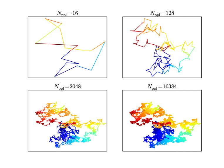
Figure 12.1: A single discrete worldline loop shown at several levels of discretization. The loops form fractal patterns and have a strong parallel with Brownian motion. The colour represents the phase of a particle travelling along the loop, and begins at dark blue, progresses in a random walk through yellow, and ends at dark red. The total flux through this particular worldline at $T=1$ and $B=B_{k}$ is about $0.08\pi/e$.

Cylindrical Worldline Numerics

We now consider cylindrically symmetric external magnetic fields. In this case, we may simplify (12.1),

$$\frac{\Gamma^{(1)}_{\rm ferm}}{TL_{z}}=\frac{1}{4\pi}\int_{0}^{\infty}\rho_{\rm cm}\left[\int_{0}^{\infty}\frac{dT}{T^{3}}e^{-m^{2}T}\left\{\langle W\rangle_{{\bf r}_{\rm cm}}-1-\frac{1}{3}(eB_{\rm cm}T)^{2}\right\}\right]d\rho.$$ (12.15)

Cylindrical Magnetic Fields

We have ${\bf B}=B(\rho)$${\bf\hat{z}}$ with

$$B(\rho)=\frac{A_{\phi}(\rho)}{\rho}+\frac{dA_{\phi}(\rho)}{d\rho}$$ (12.16)

if we make the gauge choice that $A_{0}=A_{\rho}=A_{z}=0$.

We begin by considering $A_{\phi}(\rho)$ in the form

$$A_{\phi}(\rho)=\frac{F}{2\pi\rho}f_{\lambda}(\rho)$$ (12.17)

so that

$$B_{z}(\rho)=\frac{F}{2\pi\rho}\frac{df_{\lambda}(\rho)}{d\rho}$$ (12.18)

and the total flux is

$$\Phi=F(f_{\lambda}(L_{\rho})-f_{\lambda}(0)).$$ (12.19)

It is convenient to express the flux in units of $\frac{2\pi}{e}$ and define a dimensionless quantity

$$\mathcal{F}=\frac{e}{2\pi}F.$$ (12.20)

Wilson Loop

The quantity inside the angled brackets in equation (12.1) is a gauge invariant observable called a Wilson loop. We note that the proper time integral provides a natural path ordering for this operator. The Wilson loop expectation value is

$$\langle W\rangle_{{\bf r}_{\rm cm}}=\left\langle e^{ie\int_{0}^{T}d\tau{\bf A}({\bf r}_{{\rm cm}}+{\bf r}(\tau))\cdot\dot{{\bf r}}}\frac{1}{4}{\rm tr}e^{\frac{e}{2}\int_{0}^{T}d\tau\sigma_{\mu\nu}F_{\mu\nu}({\bf r}_{{\rm cm}}+{\bf r}(\tau))}\right\rangle_{{\bf r}_{\rm cm}},$$ (12.21)

which we look at as a product between a scalar part ($e^{ie\int_{0}^{T}d\tau{\bf A}({\bf r}_{{\rm cm}}+{\bf r}(\tau))\cdot\dot{{\bf r}}}$) and a fermionic part ($\frac{1}{4}{\rm tr}e^{\frac{e}{2}\int_{0}^{T}d\tau\sigma_{\mu\nu}F_{\mu\nu}({\bf r}_{{\rm cm}}+{\bf r}(\tau))}$).

Scalar Part

In a magnetic field, the scalar part is related to the flux through the loop, $\Phi_{B}$, by Stokes theorem:

$$e^{ie\int_{0}^{T}d\tau{\bf A}\cdot\dot{{\bf r}}} = e^{ie\oint{\bf A}\cdot d{\bf r}}=e^{ie\int_{{\bf\Sigma}}{\bf\nabla}\times{\bf A}\cdot d{\bf\Sigma}}$$ (12.22)

$$= e^{ie\int_{{\bf\Sigma}}{\bf B}d{\bf\Sigma}}=e^{ie\Phi_{B}}.$$ (12.23)

So, this factor accounts for the Aharonov-Bohm phase aquired by particles in the loop.

The loop discretization results in the following approximation of the scalar integral:

$$\oint{\bf A}({\bf r})\cdot d{\bf r}=\sum_{i=1}^{N_{ppl}}\int_{{\bf r}^{i}}^{{\bf r}^{i+1}}{\bf A}({\bf r})\cdot d{\bf r}.$$ (12.24)

Using a linear parameterization of the positions, the line integrals are

$$\int_{{\bf r}^{i}}^{{\bf r}^{i+1}}{\bf A}({\bf r})\cdot d{\bf r}=\int_{0}^{1}dt{\bf A}({\bf r}(t))\cdot({\bf r}^{i+1}-{\bf r}^{i}).$$ (12.25)

Using the same gauge choice outlined above (${\bf A}=A_{\phi}\hat{\phi}$), we may write

$${\bf A}({\bf r}(t))=\frac{\mathcal{F}}{e\rho^{2}}f_{\lambda}(\rho^{2})(-y,x,0),$$ (12.26)

where we have chosen $f_{\lambda}(\rho^{2})$ to depend on $\rho^{2}$ instead of $\rho$ to simplify some expressions and to avoid taking many costly square roots in the worldline numerics. We then have

$$\int_{{\bf r}^{i}}^{{\bf r}^{i+1}}{\bf A}({\bf r})\cdot d{\bf r}=\mathcal{F}(x^{i}y^{i+1}-y^{i}x^{i+1})\int_{0}^{1}dt\frac{f_{\lambda}(\rho_{i}^{2}(t))}{\rho_{i}^{2}(t)}.$$ (12.27)

The linear interpolation in Cartesian coordinates gives

$$\rho_{i}^{2}(t)=A_{i}+2B_{i}t+C_{i}t^{2},$$ (12.28)

where

$$A_{i} = (x^{i})^{2}+(y^{i})^{2}$$ (12.29)

$$B_{i} = x^{i}(x^{i+1}-x^{i})+y^{i}(y^{i+1}-y^{i})$$ (12.30)

$$C_{i} = (x^{i+1}-x^{i})^{2}+(y^{i+1}-y^{i})^{2}.$$ (12.31)

In performing the integrals along the straight lines connecting each discretized loop point, we are in danger of violating gauge invariance. If these integrals can be performed analytically, than gauge invariance is preserved exactly. However, in general, we wish to compute these integrals numerically. In this case, gauge invariance is no longer guaranteed, but can be preserved to any numerical precision that’s desired.

Fermion Part

For fermions, the Wilson loop is modified by a factor,

$$W^{\rm ferm.} = \frac{1}{4}{\rm tr}\left(e^{\frac{1}{2}e\int_{0}^{T}d\tau\sigma_{\mu\nu}F^{\mu\nu}}\right)$$ (12.32)

$$= \frac{1}{4}{\rm tr}\left(e^{\sigma_{xy}e\int_{0}^{T}d\tau B\left(x(\tau)\right)}\right)$$ (12.33)

$$= \cosh{\left(e\int_{0}^{T}d\tau B\left(x(\tau)\right)\right)}$$ (12.34)

$$= \cosh{\left(2\mathcal{F}\int_{0}^{T}d\tau f^{\prime}_{\lambda}(\rho^{2}(\tau))\right)},$$ (12.35)

where I have used the relation

$$eB=2\mathcal{F}\frac{df_{\lambda}(\rho^{2})}{d\rho^{2}}=2\mathcal{F}f^{\prime}_{\lambda}(\rho^{2}).$$ (12.36)

This factor represents an additional contribution to the action because of the spin interaction with the magnetic field. Classically, for a particle with a magnetic moment ${\bf\mu}$ travelling through a magnetic field in a time $T$, the action is modified by a term given by

$$\Gamma^{0}_{\rm spin}=\int_{0}^{T}{\bf\mu}\cdot{\bf B}({\bf x}(\tau))d\tau.$$ (12.37)

The magnetic moment is related to the electron spin ${\bf\mu}=g\left(\frac{e}{2m}\right){\bf\sigma}$, so we see that the integral in the above quantum fermion factor is very closely related to the classical action associated with transporting a magnetic moment through a magnetic field:

$$\Gamma^{0}_{\rm spin}=g\left(\frac{e}{2m}\right)\sigma_{xy}\int_{0}^{T}B_{z}(x(\tau))d\tau.$$ (12.38)

Qualitatively, we could write

$$W^{\rm ferm}\sim\cosh{\left(\Gamma^{0}_{\rm spin}\right)}.$$ (12.39)

As a possibly useful aside, we may want to express the integral in terms of $f_{\lambda}(\rho^{2})$ instead of its derivative. We can do this by integrating by parts:

$$\int_{0}^{T}d\tau f^{\prime}_{\lambda}(\rho^{2}(\tau)) = \frac{T}{N_{\rm ppl}}\sum_{i=1}^{N_{\rm ppl}}\int_{0}^{1}dtf^{\prime}_{\lambda}(\rho^{2}_{i}(\tau))$$ (12.41)

$$= \frac{T}{N_{\rm ppl}}\sum_{i=1}^{N_{\rm ppl}}\biggr{[}\frac{f_{\lambda}(\rho^{2}_{i}(t))}{2(B_{i}+C_{i}t)}\biggr{|}^{t=1}_{t=0}$$

$$+\frac{C_{i}}{2}\int_{0}^{1}\frac{f_{\lambda}(\rho^{2}_{i}(t))}{(B_{i}+C_{i}t)^{2}}dt\biggr{]}$$

$$= \frac{T}{N_{\rm ppl}}\sum_{i=1}^{N_{\rm ppl}}\frac{C_{i}}{2}\int_{0}^{1}\frac{f_{\lambda}(\rho^{2}_{i}(t))}{(B_{i}+C_{i}t)^{2}}dt,$$ (12.42)

with $\rho_{i}^{2}(t)$ given by equations (12.28) to (12.31). The second equality is obtained from integration-by-parts. In the third equality, we use the loop sum to cancel the boundary terms in pairs:

$$W^{{\rm ferm.}}=\cosh{\left(\frac{\mathcal{F}T}{N_{\rm ppl}}\sum_{i=1}^{N_{{\rm ppl}}}C_{i}\int_{0}^{1}dt\frac{f_{\lambda}(\rho^{2}_{i}(t))}{(B_{i}+C_{i}t)^{2}}\right)}.$$ (12.43)

In most cases, one would use equation (12.35) to compute the fermion factor of the Wilson loop. However, equation (12.43) may be useful in cases where $f^{\prime}_{\lambda}(\rho^{2}(\tau))$ is not known or is difficult to compute.

Renormalization

The field strength renormalization counter-terms result from the small $T$ behaviour of the worldline integrand. In the limit where $T$ is very small, the worldline loops are very localized around their center of mass. So, we may approximate their contribution as being that of a constant field with value ${\bf A}({\bf r}_{{\rm cm}})$. Specifically, we require that the field change slowly on the length scale defined by $\sqrt{T}$. This condition on $T$ can be written

$$T\ll\left|\frac{m^{2}}{eB^{\prime}(\rho^{2})}\right|=\left|\frac{m^{2}}{2\mathcal{F}f^{\prime\prime}_{\lambda}(\rho^{2}_{\rm cm})}\right|.$$ (12.44)

When this limit is satisfied, we may use the exact expressions for the constant field Wilson loops to determine the small $T$ behaviour of the integrands and the corresponding counter terms.

The Wilson loop averages for constant magnetic fields in scalar and fermionic $\mathrm{QED}$ are

$$\langle W\rangle_{\rm ferm}=eBT\coth{(eBT)}$$ (12.45)

and

$$\langle W\rangle_{\rm scal}=\frac{eBT}{\sinh{(eBT)}}.$$ (12.46)

So, the integrand for fermionic $\mathrm{QED}$ in the limit of small $T$ is

$$I_{\rm ferm}(T) = \frac{e^{-m^{2}T}}{T^{3}}\left[eB({\bf r}_{cm})T\coth{(eB({\bf r}_{cm})T)}-1-\frac{e^{2}}{3}B^{2}({\bf r}_{cm})T^{2}\right]$$ (12.47)

$$\approx -\frac{(eB)^{4}T}{45}+\frac{1}{45}(eB)^{4}m^{2}T^{2}+\left(\frac{2(eB)^{6}}{945}-\frac{(eB)^{4}m^{4}}{90}\right)T^{3}$$

$$+\frac{(7(eB)^{4}m^{6}-4(eB)^{6}m^{2})T^{4}}{1890}+O(T^{5}).$$

For scalar quantum electrodynamics ($\mathrm{ScQED}$), we have

$$I_{\rm scal}(T) = \frac{e^{-m^{2}T}}{T^{3}}\left[eB({\bf r}_{cm})T/\sinh{(eB({\bf r}_{cm})T)}-1+\frac{1}{6}(eB)^{2}({\bf r}_{cm})T^{2}\right]$$ (12.48)

$$\approx \frac{7(eB)^{4}T}{360}-\frac{7(eB)^{4}m^{2}T^{2}}{360}+\frac{(147(eB)^{4}m^{4}-31(eB)^{6})T^{3}}{15120}$$

$$+\frac{(31(eB)^{6}m^{2}-49(eB)^{4}m^{6})T^{4}}{15120}+O(T^{5}).$$

Beyond providing the renormalization conditions, these expansions can be used in the small $T$ regime to avoid a problem with the Wilson loop uncertainties in this region. Consider the uncertainty in the integrand arising from the uncertainty in the Wilson loop:

$$\delta I(T) = \frac{\partial I}{\partial W}\delta W$$ (12.49)

$$= \frac{e^{-m^{2}T}}{T^{3}}\delta W.$$ (12.50)

In this case, even though we can compute the Wilson loops for small $T$ precisely, even a small uncertainty is magnified by a divergent factor when computing the integrand for small values of $T$. So, in order to perform the integral, we must replace the small $T$ behaviour of the integrand with the above expansions (12.47) and (12.48). Our worldline integral then proceeds by analytically computing the integral for the small $T$ expansion up to some small value, $a$, and adding this to the remaining part of the integral [144]:

$$\int_{0}^{\infty}I(T)dT=\underbrace{\int_{0}^{a}I(T)dT}_{\rm small~{}T}+\underbrace{\int_{a}^{\infty}I(T)dT}_{\rm worldline~{}numerics}.$$ (12.51)

Because this normalization proceedure uses the constant field expressions for small values of $T$, this scheme introduces a small systematic uncertainty. To improve on the method outlined here, the derivatives of the background field can be accounted for by using the analytic forms of the heat kernel expansion to perform the renormalization [57].

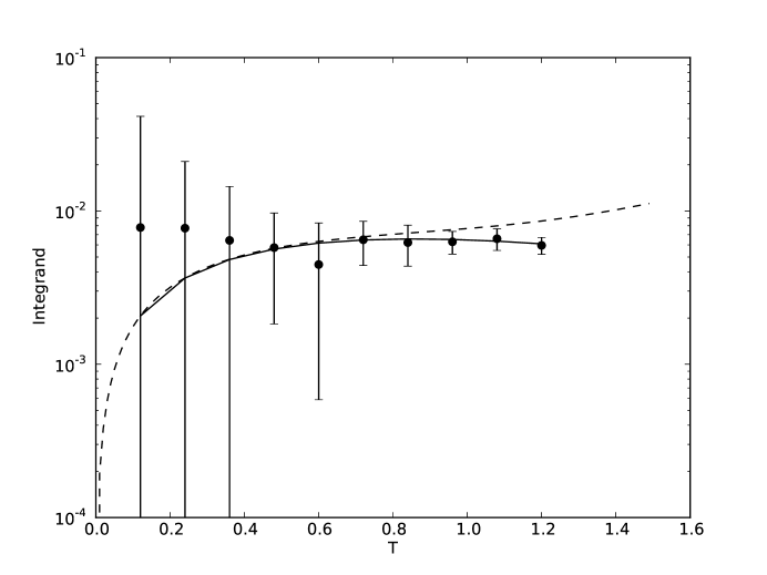
Figure 12.2: The small $T$ behaviour of $\mathrm{WLN}$. The data points represent the numerical results, where the error bars are determined from the jackknife analysis described in chapter 13. The solid line represents the exact solution while the dotted line represents the small $T$ expansion of the exact solution. Note the amplification of the uncertainties.

Computing an Effective Action

The ensemble average in the effective action is simply the sum over the contributions from each worldline loop, divided by the number of loops in the ensemble. Since the computation of each loop is independent of the other loops, the ensemble average may be straightforwardly parallelized by generating separate processes to compute the contribution from each loop. For this parallelization, four Nvidia Tesla C1060 $\mathrm{GPU}$s were used through the $\mathrm{CUDA}$ parallel programing framework. Because $\mathrm{GPU}$s can spawn thousands of parallel processing threads with much less computational overhead than an message passing interface ($\mathrm{MPI}$) cluster, they excel at handling a very large number of parallel threads, although the clock speed is slower and fewer memory resources are typically available. In contrast, parallel computing on a cluster using $\mathrm{CPU}$ tends to have a much higher speed per thread, but there are typically fewer threads available. The worldline technique is exceedingly parallelizable, and it is a straightforward matter to divide the task into thousands or tens of thousands of parallel threads. In this case, one should expect excellent performance from a $\mathrm{GPU}$ over a parallel central processing unit ($\mathrm{CPU}$) implementation, unless thousands of $\mathrm{CPU}$s are available for the program. The $\mathrm{GPU}$ architecture has recently been used by another group for computing Casimir forces using worldline numerics [3]. Figure 12.3 illustrates the coprocessing and parallelization scheme used here for the worldline numerics.

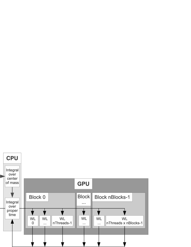
Figure 12.3: The $\mathrm{CPU}$ manages the loops which compute the integrals over center of mass and proper time. For each proper time integral, we require the results from a large number of individual worldlines. The $\mathrm{GPU}$ is used to compute the integral over each worldline in parallel, and the results are returned to the $\mathrm{CPU}$ for use in the effective action calculation.

.

In an informal test, a Wilson loop average was computed using an ensemble of 5000 loops in 4.7553 seconds using a serial implementation while the $\mathrm{GPU}$ performed the same calculation in 0.001315 seconds using a $\mathrm{CUDA}$ implementation. A parallel $\mathrm{CPU}$ code would require a cluster with thousands of cores to achieve a similar speed, even if we assume linear (ideal) speed-up. So, for $\mathrm{WLN}$ computations, a relatively inexpensive $\mathrm{GPU}$ can be expected to outperform a small or mid-sized cluster. This increase in computation speed has enabled the detailed parameter searches discussed in this dissertation.

Of course, there are also tradeoffs from using the $\mathrm{GPU}$ architecture with the $\mathrm{WLN}$ technique. The most significant of these is the limited availability of memory on the device. A $\mathrm{GPU}$ device provides only a few GB of global memory (4GB on the Tesla C1060). This limit forces compromises between the number of points-per-loop and the number of loops to keep the total size of the loop cloud data small. The limited availability of memory resources also limits the number of threads which can be executed concurrently on the device. Because of the overhead associated with transfering data to and from the device, the advantages of a $\mathrm{GPU}$ over a $\mathrm{CPU}$ cluster are most pronounced on problems which can be divided into several hundred or thousands of processes. Therefore, the $\mathrm{GPU}$ may not offer great performance advantages for a small number of loops. Finally, there is some additional complexity involved in programming for the $\mathrm{GPU}$ in terms of learning specialized libraries and memory management on the device. This means that the code may take longer to develop and there may be a learning curve for researchers. However, this problem is not much more pronounced with $\mathrm{GPU}$ programming than with other parallelization strategies.

Once the ensemble average of the Wilson loop has been computed, computing the effective action is a straightforward matter of performing numerical integrals. The effective action density is computed by performing the integration over proper time, $T$. Then, the effective action is computed by performing a spacetime integral over the loop ensemble center of mass. In all cases where a numerical integral was performed, Simpson’s method was used [21]. Integrals from 0 to $\infty$ were mapped to the interval $[0,1]$ using substitutions of the form $x=\frac{1}{1+T/T_{\rm max}}$, where $T_{\rm max}$ sets the scale for the peak of the integrand. In the constant field case, for the integral over proper time, we expect $T_{\rm max}\sim 3/(eB)$ for large fields and $T_{\rm max}\sim 1$ for fields of a few times critical or smaller. In chapter 13, we present a detailed discussion of how the statistical and discretization uncertainties can be computed in this technique.

In this implementation, the numerical integrals are done using a serial CPU computation. This serial portion of the algorithm tends to limit the speedup that can be achieved with the large number of parallel threads on the $\mathrm{GPU}$ device. However, an important benefit of the large number of threads available on the $\mathrm{GPU}$ is that the number of worldlines in the ensemble can be increased without limit, as long as more threads are available, without significantly increasing the computation time. If perfect occupancy could be achieved on a Tesla C1060 device, an ensemble of up to 30,720 worldlines could be computed concurrently. Thus, the $\mathrm{GPU}$ provides an excellent architecture for improving the statistical uncertainties. Additionally, there is room for further optimization of the algorithm by parallelizing the serial portions of the algorithm to achieve a greater speedup.

More details about implementing this algorithm on the $\mathrm{CUDA}$ architecture can be found in appendix A. A listing of the $\mathrm{CUDA}$ $\mathrm{WLN}$ code appears in appendix B.

Verification and Validation

The $\mathrm{WLN}$ software can be validated and verified by making sure that it produces the correct results where the derivative expansion is a good approximation, and that the results are consistent with previous numerical calculations of flux tube effective actions. For this reason, the validation was done primarily with flux tubes with a profile defined by the function

$$f_{\lambda}(\rho^{2})=\frac{\rho^{2}}{(\lambda^{2}+\rho^{2})}.$$ (12.52)

For large values of $\lambda$, this function varies slowly on the Compton wavelength scale, and so the derivative expansion is a good approximation. Also, flux tubes with this profile were studied previously using $\mathrm{WLN}$ [145, 144].

Among the results presented in [144] is a comparison of the derivative expansion and $\mathrm{WLN}$ for this magnetic field configuration. The result is that the next-to-leading-order term in the derivative expansion is only a small correction to the the leading-order term for $\lambda\gg\lambda_{e}$, where the derivative expansion is a good approximation. The derivative expansion breaks down before it reaches its formal validity limits at $\lambda\sim\lambda_{e}$. For this reason, we will simply focus on the leading order derivative expansion (which we call the locally constant field ($\mathrm{LCF}$) approximation). The effective action of $\mathrm{QED}$ in the $\mathrm{LCF}$ approximation is given in cylindrical symmetry by

$$\Gamma^{(1)}_{\rm ferm} = \frac{1}{4\pi}\int_{0}^{\infty}dT\int_{0}^{\infty}\rho_{\rm cm}d\rho_{\rm cm}\frac{e^{-m^{2}T}}{T^{3}}$$ (12.53)

$$\left\{eB(\rho_{\rm cm})T\coth{(eB(\rho_{\rm cm})T)}-1-\frac{1}{3}(eB(\rho_{\rm cm})T)^{2}\right\}.$$

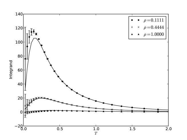
Figure 12.4: The integrand of the proper time, $T$, integral for three different values of the radial coordinate, $\rho$ for a $\lambda=1$ flux tube. The solid lines represent the zeroth-order derivative expansion, which, as expected, is a good approximation until $\rho$ becomes too small.

Figure 12.4 shows a comparison between the proper time integrand,

$$\frac{e^{-m^{2}T}}{T^{3}}\left[\langle W\rangle_{{\bf r}_{\rm cm}}-1-\frac{1}{3}(eB_{\rm cm}T)^{2}\right],$$ (12.54)

and the $\mathrm{LCF}$ approximation result for a flux tube with $\lambda=\lambda_{e}$ and $\mathcal{F}=10$. In this case, the $\mathrm{LCF}$ approximation is only appropriate far from the center of the flux tube, where the field is not changing very rapidly. In the figure, we can begin to see the deviation from this approximation, which gets more pronounced closer to the center of the flux tube (smaller values of $\rho$).

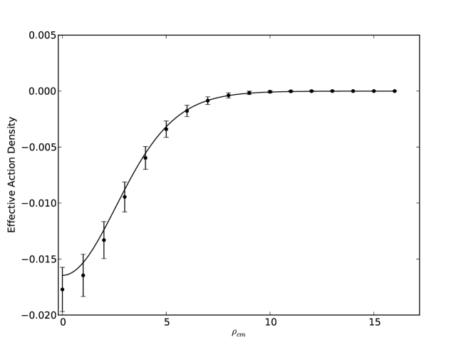
Figure 12.5: The fermion term of the effective action density as a function of the radial coordinate for a flux tube with width $\lambda=10\lambda_{e}$.

The effective action density for a slowly varying flux tube is plotted in figure 12.5 along with the $\mathrm{LCF}$ approximation. In this case, the $\mathrm{LCF}$ approximation agrees within the statistics of the $\mathrm{WLN}$.

Conclusions

In this chapter, I have reviewed the $\mathrm{WLN}$ numerical technique with a focus on computing the effective action of $\mathrm{QED}$ in nonhomogeneous, cylindrically symmetric magnetic fields. The method uses a Monte Carlo generated ensemble of worldline loops to approximate a path integral in the worldline formalism. These worldline loops are generated using a simple algorithm and encode the information about the magnetic field by computing the flux through the loop and the action aquired from transporting a magnetic moment around the loop. This technique preserves Lorentz symmetry exactly and can preserve gauge symmetry up to any required precision.

I have discussed implementing this technique on $\mathrm{GPU}$ architecture using $\mathrm{CUDA}$. The main advantage of this architecture is that it allows for a very large number of concurrent threads which can be utilized with very little overhead. In practice, this means that a large ensemble of worldlines can be computed concurrently, thus allowing for a considerable speedup over serial implementations, and allowing for the precision of the numerics to increase according to the number of threads available.

Chapter 13 Uncertainty analysis in worldline numerics

This chapter gives a brief overview of uncertainty analysis in the $\mathrm{WLN}$ method. There are uncertainties from discretizing each loop, and from using a statistical ensemble of representative loops. The former can be minimized so that the latter dominates. However, determining the statistical uncertainties is complicated by two subtleties. Firstly, the distributions generated by the worldline ensembles are highly non-Gaussian, and so the standard error in the mean is not a good measure of the statistical uncertainty. Secondly, because the same ensemble of worldlines is used to compute the Wilson loops at different values of $T$ and $x_{\rm cm}$, the uncertainties associated with each computed value of the integrand are strongly correlated. I recommend a form of jackknife analysis which deals with both of these problems.

So far in the $\mathrm{WLN}$ literature, the discussions of uncertainty analysis has been unfortunately brief. It has been suggested that the standard deviation of the worldlines provides a good measure of the statistical error in the worldline method [56, 57]. However, the distributions produced by the worldline ensemble are highly non-Gaussian, and therefore the standard error in the mean is not a good measure of the uncertainties involved. Furthermore, the use of the same worldline ensemble to compute the Wilson loop multiple times in an integral results in strongly correlated uncertainties. Thus, propagating uncertainties through integrals can be computationally expensive due to the complexity of computing correlation coefficients.

The error bars on worldline calculations impact the conclusions that can be drawn from calculations, and also have important implications for the fermion problem, which limits the domain of applicability of the technique (see section 13.3). It is therefore important that the error analysis is done thoughtfully and transparently. The purpose of this chapter is to contribute a more thorough discussion of uncertainty analysis in the $\mathrm{WLN}$ technique to the literature in hopes of avoiding any confusion associated with the above-mentioned subtleties.

There are two sources of uncertainty in the worldline technique: the discretization error in treating each continuous worldline as a set of discrete points, and the statistical error of sampling a finite number of possible worldlines from a distribution. In this chapter, I will discuss each of these sources of uncertainty.

Estimating the Discretization Uncertainties

The discretization error arising from the integral over $\tau$ in the exponent of each Wilson loop (see equation (12.21)) is difficult to estimate since any number of loops could be represented by each choice of discrete points. The general strategy is to make this estimation by computing the Wilson loop using several different numbers of points per worldline and observing the convergence properties.

The specific procedure adopted for this work involves dividing each discrete worldline into several worldlines with varying levels of discretization. Since we are using the d-loop method for generating the worldlines (section 12.2.1), a $\frac{N_{ppl}}{2}$ sub-loop consisting of every other point will be guaranteed to contain the prescribed distribution of velocities.

To look at the convergence for the loop discretization, each worldline is divided into three groups. One group of $\frac{N_{ppl}}{2}$ points, and two groups of $\frac{N_{ppl}}{4}$. This permits us to compute the average holonomy factors at three levels of discretization:

$$\langle W\rangle_{N_{ppl}/4}=\langle e^{\frac{i}{2}\triangle}e^{\frac{i}{2}\Box}\rangle,$$ (13.1)

$$\langle W\rangle_{N_{ppl}/2}=\langle e^{i\circ}\rangle,$$ (13.2)

and

$$\langle W\rangle_{N_{ppl}}=\langle e^{\frac{i}{2}\circ}e^{\frac{i}{4}\Box}e^{\frac{i}{4}\triangle}\rangle,$$ (13.3)

where the symbols $\circ$, $\Box$, and $\triangle$ denote the worldline integral, $\int_{0}^{T}d\tau A(x_{CM}+x(\tau))\cdot\dot{x}$, computed using the sub-worldlines depicted in figure 13.1.

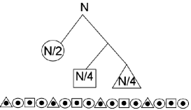
Figure 13.1: Diagram illustrating the division of a worldline into three smaller interleaved worldlines

We may put these factors into the equation of a parabola to extrapolate the result to an infinite number of points per line (see figure 13.2):

$$\langle W\rangle_{\infty}\approx\frac{8}{3}\langle W\rangle_{N_{ppl}}-2\langle W\rangle_{N_{ppl}/2}+\frac{1}{3}\langle W\rangle_{N_{ppl}/4}.$$ (13.4)

So, we estimate the discretization uncertainty to be

$$\delta\langle W\rangle_{\infty}\approx|\langle W\rangle_{N_{ppl}}-\langle W\rangle_{\infty}|.$$ (13.5)

Generally, the statistical uncertainties are the limitation in the precision of the $\mathrm{WLN}$ technique. Therefore, $N_{ppl}$ should be chosen to be large enough that the discretization uncertainties are small relative to the statistical uncertainties.

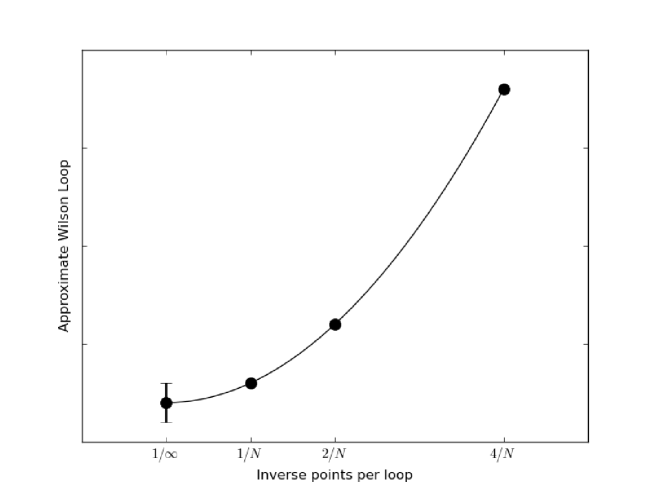
Figure 13.2: This plot illustrates the method used to extrapolate the Wilson loop to infinite points per loop and the uncertainty estimate in the approximation.

Estimating the Statistical Uncertainties

We can gain a great deal of insight into the nature of the statistical uncertainties by examining the specific case of the uniform magnetic field since we know the exact solution in this case.

The Worldline Ensemble Distribution is Non-Gaussian

A reasonable first instinct for estimating the error bars is to use the standard error in the mean of the collection of individual worldlines:

$${\rm SEM}(W)=\sqrt{\sum_{i=1}^{N_{l}}\frac{(W_{i}-\langle W\rangle)^{2}}{N_{l}(N_{l}-1)}}.$$ (13.6)

This approach has been promoted in early papers on $\mathrm{WLN}$ [56, 57]. In figure 13.3, I have plotted the residuals and the corresponding error bars for several values of the proper time parameter, $T$. From this plot, it appears that the error bars are quite large in the sense that we appear to produce residuals which are considerably smaller than would be implied by the sizes of the error bars. This suggests that we have overestimated the size of the uncertainty.

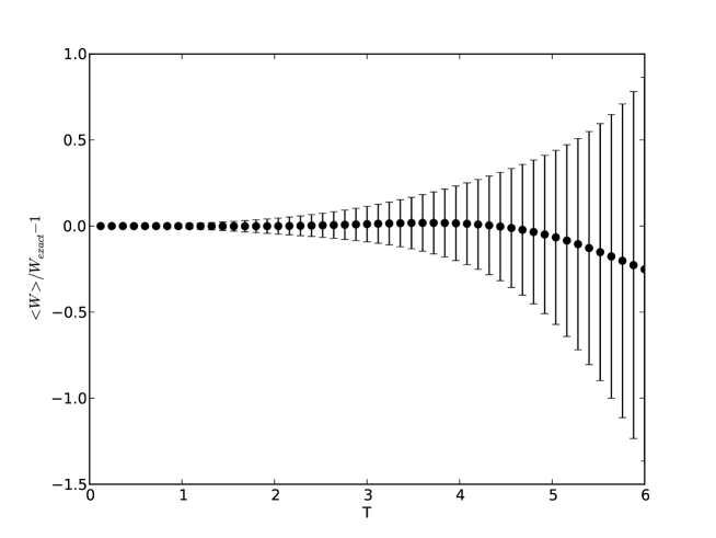
Figure 13.3: Residuals of worldline calculations and the corresponding standard errors in the mean. For reasons discussed in this section, these error bars overestimate the uncertainties involved.

We can see why this is the case by looking more closely at the distributions produced by the worldline technique. An exact expression for these distributions can be derived in the case of the constant magnetic field [144]:

$$w(y)=\frac{W_{\rm exact}}{\sqrt{1-y^{2}}}\sum_{-\infty}^{\infty}[f(\arccos(y)+2n\pi)+f(-\arccos(y)+2n\pi)]$$ (13.7)

with

$$f(\phi)=\frac{\pi}{4BT\cosh^{2}(\frac{\pi\phi}{2BT})}.$$ (13.8)

Figure 13.4 shows histograms of the worldline results along with the expected distributions. These distributions highlight a significant hurdle in assigning error bars to the results of $\mathrm{WLN}$.

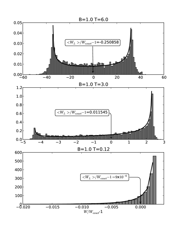
Figure 13.4: Histograms showing the worldline distributions of the residuals for three values of $T$ in the constant magnetic field case. Here, we are neglecting the fermion factor. The dark line represents the exact distribution computed using equation 13.7. The worldline means are indicated with an arrow, while the exact mean in each case is 0. There are 5120 worldlines in each histogram. The vertical axes are normalized to a total area of unity.

Due to their highly non-Gaussian nature, the standard error in the mean is not a good characterization of the distributions that are produced. We should not interpret each individual worldline as a measurement of the mean value of these distributions; for large values of $BT$, almost all of our worldlines will produce answers which are far away from the mean of the distribution. This means that the variance of the distribution will be very large, even though our ability to determine the mean of the distribution is relatively precise because of the increasing symmetry about the mean as $T$ becomes large.

Correlations between Wilson Loops

Typically, numerical integration is performed by replacing the integral with a sum over a finite set of points from the integrand. So, I will begin the present discussion by considering the uncertainty in adding together two points (labelled $i$ and $j$) in our integral over $T$. Two terms of the sum representing the numerical integral will involve a function of $T$ times the two Wilson loop factors,

$$I=g(T_{i})\langle W(T_{i})\rangle+g(T_{j})\langle W(T_{j})\rangle$$ (13.9)

with an uncertainty given by

$$\delta I = \left|\frac{\partial I}{\partial\langle W(T_{i})\rangle}\right|^{2}(\delta\langle W(T_{i})\rangle)^{2}+\left|\frac{\partial I}{\partial\langle W(T_{j})\rangle}\right|^{2}(\delta\langle W(T_{j})\rangle)^{2}$$ (13.11)

$$+2\left|\frac{\partial I}{\partial\langle W(T_{i})\rangle}\frac{\partial I}{\partial\langle W(T_{j})\rangle}\right|\rho_{ij}(\delta\langle W(T_{i})\rangle)(\delta\langle W(T_{j})\rangle)$$

$$= g(T_{i})^{2}(\delta\langle W(T_{i})\rangle)^{2}+g(T_{j})^{2}(\delta\langle W(T_{j})\rangle)^{2}$$

$$+2\left|g(T_{i})g(T_{j})\right|\rho_{ij}(\delta\langle W(T_{i})\rangle)(\delta\langle W(T_{j})\rangle)$$

and the correlation coefficient $\rho_{ij}$ given by

$$\rho_{ij}=\frac{\langle(W(T_{i})-\langle W(T_{i})\rangle)(W(T_{j})-\langle W(T_{j})\rangle)\rangle}{\sqrt{(W(T_{i})-\langle W(T_{i})\rangle)^{2}}\sqrt{(W(T_{j})-\langle W(T_{j})\rangle)^{2}}}.$$ (13.12)

The final term in the error propagation equation takes into account correlations between the random variables $W(T_{i})$ and $W(T_{j})$. Often in a Monte Carlo computation, one can treat each evaluation of the integrand as independent, and neglect the uncertainty term involving the correlation coefficient. However, in $\mathrm{WLN}$, the evaluations are related because the same worldline ensemble is reused for each evaluation of the integrand. So, the correlations are significant (see figure 13.5), and this term can’t be neglected. Computing each correlation coefficient takes a time proportional to the square of the number of worldlines. So, it may be computationally expensive to formally propagate uncertainties through an integral.

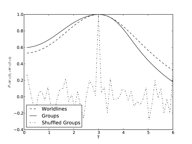
Figure 13.5: Correlation coefficients, equation (13.12), between $\langle W(T)\rangle$ and $\langle W(T=3)\rangle$ computed using individual worldlines, groups of worldlines, and shuffled groups of worldlines.

The point-to-point correlations were originally pointed out by Gies and Langfeld who addressed the problem by updating (but not replacing or regenerating) the loop ensemble in between each evaluation of the Wilson loop average [56]. This may be a good way of addressing the problem. However, in the following section, I promote a method which can bypass the difficulties presented by the correlations by treating the worldlines as a collection of worldline groups.

Grouping Worldlines

Both of the problems explained in the previous two subsections can be overcome by creating groups of worldline loops within the ensemble. Each group of worldlines then makes a statistically independent measurement of the Wilson loop average for that group. The statistics between the groups of measurements are Gaussian distributed, and so the uncertainty is the standard error in the mean of the ensemble of groups (in contrast to the ensemble of worldlines).

For example, if we divide the $N_{l}$ worldlines into $N_{G}$ groups of $N_{l}/N_{G}$ worldlines each, we can compute a mean for each group:

$$\langle W\rangle_{G_{j}}=\frac{N_{G}}{N_{l}}\sum_{i=1}^{N_{l}/N_{G}}W_{i}.$$ (13.13)

Provided each group contains the same number of worldlines, the average of the Wilson loop is unaffected by this grouping:

$$\langle W\rangle = \frac{1}{N_{G}}\sum_{j=1}^{N_{G}}\langle W\rangle_{G_{j}}$$ (13.14)

$$= \frac{1}{N_{l}}\sum_{i=1}^{N_{l}}W_{i}.$$ (13.15)

However, the uncertainty is the standard error in the mean of the groups,

$$\delta\langle W\rangle=\sqrt{\sum_{i=1}^{N_{G}}\frac{(\langle W\rangle_{G_{i}}-\langle W\rangle)^{2}}{N_{G}(N_{G}-1)}}.$$ (13.16)

Because the worldlines are unrelated to one another, the choice of how to group them to compute a particular Wilson loop average is arbitrary. For example, the simplest choice is to group the loops by the order they were generated, so that a particular group number, $i$, contains worldlines $iN_{l}/N_{G}$ through $(i+1)N_{l}/N_{G}-1$. Of course, if the same worldline groupings are used to compute different Wilson loop averages, they will still be correlated. We will discuss this problem in a moment.

The basic claim of the worldline technique is that the mean of the worldline distribution approximates the holonomy factor. However, from the distributions in figure 13.4, we can see that the individual worldlines themselves do not approximate the holonomy factor. So, we should not think of an individual worldline as an estimator of the mean of the distribution. Thus, a resampling technique is required to determine the precision of our statistics. We can think of each group of worldlines as making an independent measurement of the mean of a distribution. As expected, the groups of worldlines produce a more Gaussian-like distribution (see figure 13.6), and so the standard error of the groups is a sensible measure of the uncertainty in the Wilson loop value.

Figure 13.6: The histogram demonstrating the precision with which we can reproduce measurements of the mean using different groups of 100 worldlines at $BT=6.0$. In this case, the distribution is Gaussian-like and meaningful error bars can be placed on our measurement of the mean.

We find that the error bars are about one-third as large as those determined from the standard error in the mean of the individual worldlines, and the smaller error bars better characterize the size of the residuals in the constant field case (see figure 13.7). The strategy of using subsets of the available data to determine error bars is called jackknifing. Several previous papers on $\mathrm{WLN}$ have mentioned using jackknife analysis to determine the uncertainties, but without an explanation of the motivations or the procedure employed [53, 55, 41, 58].

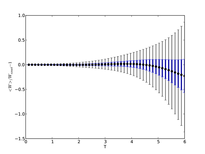
Figure 13.7: The residuals of the Wilson loops for a constant magnetic field showing the standard error in the mean (thin error bars) and the uncertainty in determining the mean (thick blue error bars). The standard error in the mean overestimates the uncertainty by more than a factor of 3 at each value of $T$.

The grouping of worldlines alone does not address the problem of correlations between different evaluations of the integrands. Figure 13.5 shows that the uncertainties for groups of worldlines are also correlated between different points of the integrand. However, the worldline grouping does provide a tool for bypassing the problem. One possible strategy is to randomize how worldlines are assigned to groups between each evaluation of the integrand. This produces a considerable reduction in the correlations, as is shown in figure 13.5. Then, errors can be propagated through the integrals by neglecting the correlation terms. Another strategy is to separately compute the integrals for each group of worldlines, and then consider the statistics of the final product to determine the error bars. This second strategy is the one adopted for the work presented in this thesis. Grouping in this way reduces the amount of data which must be propagated through the integrals by a factor of the group size compared to a delete-1 jackknife scheme, for example. In general, the error bars quoted in this thesis are obtained by computing the standard error in the mean of groups of worldlines.

Uncertainties and the Fermion Problem

The fermion problem of $\mathrm{WLN}$ is a name given to an enhancement of the uncertainties at large $T$ [56, 144]. It should not be confused with the fermion doubling problem associated with lattice methods. In a constant magnetic field, the scalar portion of the calculation produces a factor of $\frac{BT}{\sinh{(BT)}}$, while the fermion portion of the calculation produces an additional factor $\cosh{(BT)}$. Physically, this contribution arises as a result of the energy required to transport the electron’s magnetic moment around the worldline loop. At large values of $T$, we require subtle cancellation between huge values produced by the fermion portion with tiny values produced by the scalar portion. However, for large $T$, the scalar portion acquires large relative uncertainties which make the computation of large $T$ contributions to the integral very imprecise.

This can be easily understood by examining the worldline distributions shown in figure 13.4. Recall that the scalar Wilson loop average for these histograms is given by the flux in the loop, $\Phi_{B}$:

$$\langle W\rangle=\left<\exp{(ie\int_{0}^{T}d\tau{\bf A}({\bf x}_{\rm cm}+{\bf x}(\tau))\cdot d{\bf x}(\tau))}\right>=\left<e^{ie\Phi_{B}}\right>.$$ (13.17)

For constant fields, the flux through the worldline loops obeys the distribution function [144]

$$f(\Phi_{B})=\frac{\pi}{4BT\cosh^{2}\left(\frac{\pi\Phi_{B}}{2BT}\right)}.$$ (13.18)

For small values of $T$, the worldline loops are small and the amount of flux through the loop is correspondingly small. Therefore, the flux for small loops is narrowly distributed about $\Phi_{B}=0$. Since zero maximizes the Wilson loop ($e^{i0}=1$), this explains the enhancement to the right of the distribution for small values of $T$. As $T$ is increased, the flux through any given worldline becomes very large and the distribution of the flux becomes very broad. For very large $T$, the width of the distribution is many factors of $2\pi/e$. Then, the phase ($e\Phi_{B}\mod{2\pi}$) is nearly uniformly distributed, and the Wilson loop distribution reproduces the Chebyshev distribution (i.e. the distribution obtained from projecting uniformly distributed points on the unit circle onto the horizontal axis),

$$\lim_{T\to\infty}w(y)=\frac{1}{\pi\sqrt{1-y^{2}}}.$$ (13.19)

The mean of the Chebyshev distribution is zero due to its symmetry. However, this symmetry is not realized precisely unless we use a very large number of loops. Since the width of the distribution is already 100$\times$ the value of the mean at $T=6$, any numerical asymmetries in the distribution result in very large relative uncertainties of the scalar portion. Because of these uncertainties, the large contribution from the fermion factor are not cancelled precisely.

This problem makes it very difficult to compute the fermionic effective action unless the fields are well localized [144]. For example, the fermionic factor for non-homogeneous magnetic fields oriented along the z-direction is

$$\cosh{\left(e\int_{0}^{T}d\tau B(x(\tau))\right)}.$$ (13.20)

For a homogeneous field, this function grows exponentially with $T$ and is cancelled by the exponentially vanishing scalar Wilson loop. For a localized field, the worldline loops are very large for large values of $T$, and they primarily explore regions far from the field. Thus, the fermionic factor grows more slowly in localized fields, and is more easily cancelled by the rapidly vanishing scalar part.

Conclusions

In this chapter, I have identified two important considerations in determining the uncertainties associated with $\mathrm{WLN}$ computations. Firstly, the computed points within the integrals over proper time, $T$, or center of mass, ${\bf x}_{\rm cm}$, are highly correlated because one typically reuses the same ensemble of worldlines to compute each point. Secondly, the statistics of the worldlines are not Gaussian distributed and each individual worldline in the ensemble may produce a result which is very far from the mean value. So, in determining the uncertainties in the $\mathrm{WLN}$ technique, one should consider how precisely the mean of the ensemble can be measured from the ensemble and this is not necessarily given by the standard error in the mean.

These issues can be addressed simultaneously using a scheme where the worldlines from the ensemble are placed into groups and the effective action or the effective action density is evaluated separately for each group. The uncertainties can then be determined by the statistics of the groups. This scheme is less computationally intensive than a delete-1 jackknife approach because less data (by a factor of the group size) needs to be propagated through the integrals. It is also less computationally intensive than propagating the uncertainties through the numerical integrals because it avoids the computation of numerous correlation coefficients.

Chapter 14 Magnetic Flux Tubes in a Dense Lattice

If the superconducting nuclear material of a neutron star contains magnetic flux tubes, the magnetic field is likely to vary rapidly on the scales where $\mathrm{QED}$ effects are important. In this chapter, I construct a cylindrically symmetric toy model of a flux tube lattice in which the influence of neighbouring flux tubes is taken into account. We compute the effective action densities using the $\mathrm{WLN}$ technique. The numerics predict a greater effective energy density in the region of the flux tube, but a smaller energy density in the regions between the flux tubes compared to a locally-constant-field approximation. We also compute the interaction energy between a flux tube and its neighbours as the lattice spacing is reduced from infinity. Because our flux tubes exhibit compact support, this energy is entirely non-local and predicted to be zero in local approximations such as the derivative expansion. This quantity can take positive or negative values depending on the magnetic field profile and the specific definition of the interaction energy.

Introduction

Computing the quantum effective action for magnetic flux tube configurations is a problem that has generated considerable interest and has been explored through a variety of approaches [74, 174, 18, 49, 15, 165, 155, 14, 64, 197, 198, 114] (see section 10.7). Partly, this is because it is a relatively simple problem for analyzing non-homogeneous generalizations of the Heisenberg-Euler action and for exploring limitations of techniques such as the derivative expansion. But, this is also a physically important problem because tubes of magnetic flux are very important for the quantum mechanics of electrons due to the Aharonov-Bohm effect, and they appear in a variety of interesting physical scenarios such as stellar astrophysics, cosmic strings, in superconductor vortices, and quark confinement [66].

In the present context, we are concerned with the role that magnetic flux tubes play in the superconducting nuclear material of compact stars. In this scenario, the $\mathrm{QED}$ effects are particularly interesting because the magnetic flux tubes, if they exist, are confined to tubes which may be only a few percent of the Compton wavelength, $\lambda_{\rm C}$, in radius. Specifically, the flux must be confined to within the London penetration depth of the superconducting material, which for neutron stars has been estimated to be 80 fm $=$ 0.032 $\lambda_{e}$ [120]. Moreover, the flux tube density is expected to be proportional to the average magnetic field. For a background field near the quantum critical strength, $B_{k}$, such as in a neutron star, the distance between flux tubes is comparable to a Compton wavelength. This Compton wavelength scale is also the scale at which the non-locality of $\mathrm{QED}$ becomes important and at which powerful local techniques like the derivative expansion are no longer appropriate for computing the effective action.

The free energy associated with these flux tubes is a factor in determining whether the nuclear material of a neutron star is a type-I or type-II superconductor. The free energy of a flux tube is determined by looking at the energies associated with the magnetic field, with the creation of a non-superconducting region in the superconductor, and with interactions between the flux tubes. Flux tubes can only form if it is energetically favourable to do so compared to expelling the field due to the Meissner effect. In this chapter, I would like to explore the contribution from $\mathrm{QED}$ to this free energy. For an isolated flux tube, this is an additional source of energy for creating the magnetic field. For a lattice of flux tubes, there is also an energy contribution from the presence of neighbouring flux tubes because of the non-local nature of quantum field theory.

The energy of two flux tubes has been previously computed using $\mathrm{WLN}$ methods and for flux tubes with aligned fields, the energy is larger than twice the energy of a single flux tube when the flux tubes are closely spaced [114]. This result implies that there is a repulsive interaction between the flux tubes due to $\mathrm{QED}$ effects, strengthening the likelihood of the type-II scenario in neutron stars. This interaction energy increases as the flux tubes are placed closer together, and can have a similar magnitude as the $\mathrm{QED}$ correction to the energy when the flux tubes are closely spaced.

In this chapter, I will further explore the nature of this phenomenon in $\mathrm{QED}$ using a highly parallel implementation of the $\mathrm{WLN}$ technique implemented on a $\mathrm{GPU}$ architecture. Specifically, I explore cylindrically symmetric magnetic field profiles for isolated flux tubes and periodic profiles designed to model properties of a triangular lattice. This algorithm cannot be applied to spinor $\mathrm{QED}$ calculations in our model lattice because of the well-known fermion problem of $\mathrm{WLN}$. However, the problem does not affect $\mathrm{ScQED}$ calculations. Therefore, we explore the quantum-corrected energies of isolated flux tubes for both scalar and spinor electrons and use this comparison to speculate about the relationship of our cylindrical lattice model and the spinor $\mathrm{QED}$ energies of an Abrikosov lattice of flux tubes that may be found in neutron stars.

Cylindrical Magnetic Fields

We consider our flux tubes to have cylindrical symmetry so that the field points along the ${\bf\hat{z}}$-direction with a profile that depends on the radial coordinate, $\rho$. In this case, we have ${\bf B}=B(\rho)$${\bf\hat{z}}$. We can find the magnetic field in terms of the vector potential from ${\bf B}={\nabla}\times{\bf A}$ and the gauge choice that $A_{0}=A_{\rho}=A_{z}=0$. Then,

$$B(\rho)=\frac{A_{\phi}(\rho)}{\rho}+\frac{dA_{\phi}(\rho)}{d\rho}.$$ (14.1)

The vector potential, $A_{\phi}(\rho)$, can be characterized by a profile function, $f_{\lambda}$, and a dimensionless flux parameter, $\mathcal{F}=\frac{e}{2\pi}F$:

$$A_{\phi}(\rho)=\frac{\mathcal{F}}{e\rho}f_{\lambda}(\rho).$$ (14.2)

If we choose $f_{\lambda}(\rho=0)=0$, then the total flux within in a radius of $L_{\rho}$ is

$$\Phi=\frac{2\pi}{e}\mathcal{F}f_{\lambda}(L_{\rho}).$$ (14.3)

In terms of the profile function, the magnetic field is written

$$B_{z}(\rho)=\frac{\mathcal{F}}{e\rho}\frac{df_{\lambda}(\rho)}{d\rho}=\frac{2\mathcal{F}}{e}\frac{df_{\lambda}(\rho^{2})}{d(\rho^{2})}.$$ (14.4)

Isolated Flux Tubes

To explore isolated magnetic flux tubes, we consider the following profile function:

$$f_{\lambda}(\rho^{2})=\frac{\rho^{2}}{\rho^{2}+\lambda^{2}}.$$ (14.5)

From equation (14.4), this give a magnetic field with a profile

$$B_{z}(\rho^{2})=\frac{2\mathcal{F}}{e}\frac{\lambda^{2}}{(\rho^{2}+\lambda^{2})^{2}}.$$ (14.6)

This profile is a smooth flux tube representation that can be evaluated quickly. Moreover, flux tubes with this profile were studied previously using $\mathrm{WLN}$ [145, 144].

Cylindrical Model of a Flux Tube Lattice

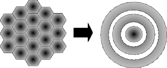
Figure 14.1: In a type-II superconductor, there are neighbouring flux tubes arranged in a hexagonal Abrikosov lattice which have a nonlocal impact on the effective action of the central flux tube (left). In our model, we account for the contributions from these neighbouring flux tubes in cylindrical symmetry by including surrounding rings of flux (right).

In a neutron star, we do not have isolated flux tubes. The tubes are likely arranged in a dense lattice with the spacing between tubes on the order of the Compton wavelength, with the size of a flux tube a few percent of the Compton wavelength. Specifically, the maximum size of a flux tube is on the order of the coherence length of the superconductor, which for neutron stars has been estimated to be $\xi\approx 30$ fm [120]. This situation can be directly computed in the $\mathrm{WLN}$ technique. However, this requires us to integrate over two spatial dimensions instead of one. Moreover, it requires the use of more loops to more precisely probe the spatial configurations of the magnetic field. Despite these problems, it is very interesting to consider a dense flux tube lattice. Unlike the isolated flux tube, the wide-tube limit of the configuration doesn’t have zero field, but an average, uniform background field. If this background field is the size of the critical field, there are interesting quantum effects even in the wide-tube limit.

In this section, I build a cylindrically symmetric toy model of a hexagonal flux tube lattice. We focus on one central flux tube and treat the surrounding six flux tubes as a continuous ring with six units of flux at a distance $a$ from the central tube. The next ring will contain twelve units of flux at a distance of $2a$, etc (see figure 14.1). Because of this condition, the average strength of the field is fixed, and the field becomes uniform in the wide tube limit instead of going to zero. For small values of $\lambda$, we will have nonlocal contributions from the surrounding rings in addition to the local contributions from the central flux tube.

It is difficult to construct a model of this scenario if the flux tubes bleed into one another as they are placed close together. For example, with Gaussian flux tubes or flux tubes with the profile used in the previous section, it is difficult to increase the width of the flux tubes while accounting for the magnetic flux that bleeds out of their regions. Moreover, it is difficult to integrate these schemes to find the profile function $f_{\lambda}(\rho)$ which is needed to compute the scalar part of the Wilson loop. In order to keep each tube as a distinct entity which stays within its assigned region, we assign a smooth function with compact support to represent each tube. This is most easily done with the bump function, $\Psi(x)$, defined as

$$\Psi(x)=\begin{cases}e^{-1/(1-x^{2})}&\mbox{ for }|x|<1\\ 0&\mbox{ otherwise}\end{cases}.$$ (14.7)

This function can be viewed as a rescaled Gaussian.

We start by defining the magnetic field outside of the central flux tube. Here, the magnetic field is a constant background field, with the flux ring contributing a bump of width $\lambda$. The height of the bump must go to zero as the width of the flux tube approaches the distance between flux tubes, and should become infinite as the flux tube width goes to zero:

$$B_{z}(\rho>\frac{a}{2})=B_{\rm bg}+A\left(\frac{a-\lambda}{\lambda}\right)\left[\Psi(2(\rho-na)/\lambda)-B\right].$$ (14.8)

with $n\equiv\lfloor\frac{\rho+a/2}{a}\rfloor$.

If we require 6 units of flux in the first outer ring, 12 in the second, and so on (see figure 14.1), the size of the background field is fixed to $B_{\rm bg}=\frac{6\mathcal{F}}{ea^{2}}$. The total flux contribution due to the $\lambda$-dependent terms must be zero:

$$\int_{(n-1/2)a}^{(n+1/2)a}\rho A\left(\frac{a-\lambda}{\lambda}\right)\left[\Psi(2(\rho-na)/\lambda)-B\right]d\rho=0$$ (14.9)

$$\frac{\lambda}{2}\int_{-1}^{1}\left(\frac{\lambda}{2}x+na\right)\Psi(x)dx-Ba^{2}n=0.$$ (14.10)

This fixes the value of the constant $B$ to

$$B=\frac{q_{1}}{2}\frac{\lambda}{a}.$$ (14.11)

The numerical constant $q_{1}$ is defined by

$$q_{1}=\int_{-1}^{1}\Psi(x)dx\approx 0.443991.$$ (14.12)

For a given bump amplitude, $A$, the magnetic field will become negative if $\lambda$ becomes small enough. Therefore, we replace $A$ with its maximum value for which the field is positive if $\lambda>\lambda_{\rm min}$ for some choice of minimum flux tube size:

$$A=\frac{12\mathcal{F}}{eaq_{1}(a-\lambda_{\rm min})}.$$ (14.13)

The choice of $\lambda_{\rm min}$ sets the tube width at which the field between the flux tubes vanishes. If $\lambda<\lambda_{\rm min}$, the magnetic field between the flux tubes will point in the $-\hat{{\bf z}}$-direction.

Because we are trying to fit a hexagonal peg into a round hole, we must treat the central flux tube differently. For example, the average field inside the central region for a unit of flux, is different than the average field in the exterior region. Therefore, even when $\lambda\rightarrow a$, the field cannot be quite uniform. We consider the field in the central region to be a constant field with a bump centered at $\rho=0$:

$$B_{z}(\rho<\frac{a}{2})=A_{0}\Psi(2\rho/\lambda)+B_{0}.$$ (14.14)

The constant term, $B_{0}$ is fixed by requiring continuity with the exterior field at $\rho=a/2$:

$$B_{0}=\frac{6\mathcal{F}}{ea^{2}}\left(1-\frac{a-\lambda}{a-\lambda_{\rm min}}\right).$$ (14.15)

The bump amplitude, $A_{0}$, is fixed by fixing the flux in the central region,

$$\int_{0}^{a/2}\rho\left[A_{0}\Psi(2\rho/\lambda)+B_{0}\right]d\rho=\frac{\mathcal{F}}{e}:$$ (14.16)

$$A_{0}\left(\frac{\lambda}{2}\right)^{2}\int_{0}^{1}x\Psi(x)dx+\frac{B_{0}}{2}\left(\frac{a}{2}\right)^{2}=\frac{\mathcal{F}}{e}$$ (14.17)

$$A_{0}=\frac{4\mathcal{F}}{\lambda^{2}eq_{2}}\left(1-\frac{3}{4}\left(1-\frac{a-\lambda}{a-\lambda_{\rm min}}\right)\right),$$ (14.18)

where the numerical constant, $q_{2}$, is defined by

$$q_{2}\equiv\int_{0}^{1}x\Psi(x)dx\approx 0.0742478.$$ (14.19)

Finally, collecting together the important expressions, the cylindrically symmetric flux tube lattice model is

$$B_{z}(\rho\leq\frac{a}{2}) = \frac{4\mathcal{F}}{\lambda^{2}eq_{2}}\left(1-\frac{3}{4}\left(\frac{\lambda-\lambda_{\rm min}}{a-\lambda_{\rm min}}\right)\right)\Psi(2\rho/\lambda)$$ (14.20)

$$+\frac{6\mathcal{F}}{ea^{2}}\left(\frac{\lambda-\lambda_{\rm min}}{a-\lambda_{\rm min}}\right)$$

$$B_{z}(\rho>\frac{a}{2})=\frac{6\mathcal{F}}{ea^{2}}\left(\frac{\lambda-\lambda_{\rm min}}{a-\lambda_{\rm min}}\right)+\frac{12\mathcal{F}}{q_{1}ea\lambda}\left(\frac{a-\lambda}{a-\lambda_{\min}}\right)\Psi(2(\rho-na)/\lambda)$$ (14.21)

with

$$\Psi(x)=\begin{cases}e^{-1/(1-x^{2})}&\mbox{ for }|x|<1\\ 0&\mbox{ otherwise}\end{cases},$$ (14.22)

$$n=\left\lfloor\frac{\rho+a/2}{a}\right\rfloor,$$ (14.23)

$$q_{1}\equiv\int_{-1}^{1}\Psi(x)dx\approx 0.443991,$$ (14.24)

and

$$q_{2}\equiv\int_{0}^{1}x\Psi(x)dx\approx 0.0742478.$$ (14.25)

The magnetic field profile defined by these equations is shown in figures 14.2 and 14.3. The current density required to created fields with this profile is shown in figure 14.4.

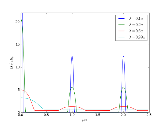
Figure 14.2: The cylindrical lattice flux tube model for several values of the width parameter $\lambda$. Here we have taken $a=\sqrt{8}\lambda_{e}$ and $\lambda_{\rm min}=0.1a$. Note that in the limit $\lambda\rightarrow a$ the field is nearly uniform with a mound in the central region. This is a consequence of the flux conditions in cylindrical symmetry requiring different fields in the internal and external regions. The height of the $\lambda=0.1a$ flux tube extends beyond the height of the graph to about $61.9B_{k}$. A 3D surface plot of the $\lambda=0.6a$ field profile is shown in figure 14.3.

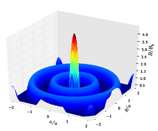
Figure 14.3: A 3D surface plot of the $\lambda=0.6a$ (red) magnetic field profile from figure 14.2.

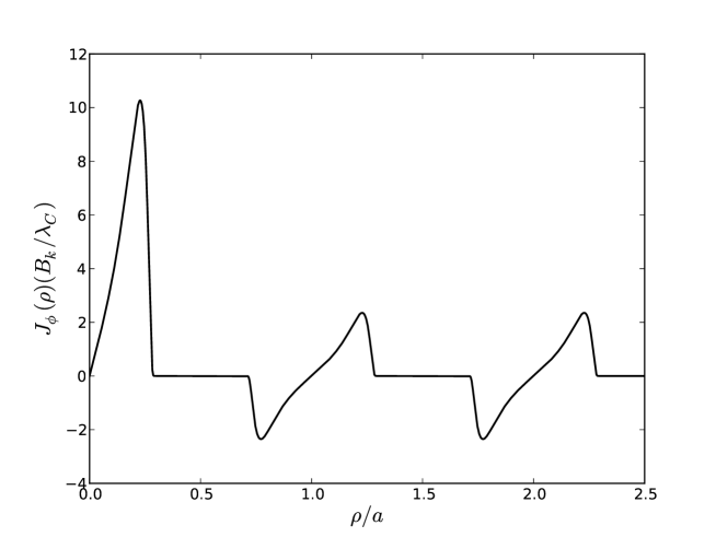
Figure 14.4: The current densities required to create the $\lambda=0.6a$ (red) magnetic field profile. The current is given by the curl of the magnetic field, $J_{\psi}(\rho)=-\frac{dB_{z}(\rho)}{d\rho}$. The conversion to SI units is $1B_{k}/\lambda_{e}\approx 6\times 10^{38}{\rm A/m}^{3}$.

The Classical Action

The classical action, $\Gamma^{0}$, is infinite for this configuration. To obtain a finite result, we must look at the action per unit length in the z-direction, per unit time, and per flux tube region (i.e. for $\rho<a/2$). The action for such a region in cylindrical coordinates is given by

$$\frac{\Gamma^{0}}{TL_{z}}=-\pi\int_{0}^{a/2}\rho B_{z}(\rho)^{2}d\rho.$$ (14.26)

We substitute in equation (14.20), the magnetic field in the interior region:

$$\frac{\Gamma^{0}}{TL_{z}} = -\pi\int_{0}^{a/2}\rho\biggr{[}\frac{4\mathcal{F}}{\lambda^{2}e^{2}q_{2}}\left(1-\frac{3}{4}\left(\frac{\lambda-\lambda_{\rm min}}{a-\lambda_{\rm min}}\right)\right)\Psi(2\rho/\lambda)$$ (14.27)

$$+\frac{6\mathcal{F}}{ea^{2}}\left(\frac{\lambda-\lambda_{\rm min}}{a-\lambda_{\rm min}}\right)\biggr{]}^{2}d\rho.$$

After some algebra, we are left with an expression for the classical action,

$$\frac{\Gamma_{0}}{TL_{z}} = \pi\int_{0}^{a/2}\rho B_{z}(\rho)^{2}d\rho$$ (14.29)

$$= -\frac{\pi\mathcal{F}^{2}}{e^{2}a^{2}}\biggr{\{}4\frac{a^{2}q_{3}}{\lambda^{2}q_{2}^{2}}+\left(\frac{\lambda-\lambda_{\rm min}}{a-\lambda_{\rm lmin}}\right)\biggr{[}$$

$$\left(\frac{9}{4}\frac{a^{2}q_{3}}{\lambda^{2}q_{2}^{2}}-\frac{9}{2}\right)\left(\frac{\lambda-\lambda_{\rm min}}{a-\lambda_{\rm lmin}}\right)-6\frac{a^{2}q_{3}}{\lambda^{2}q_{2}^{2}}+12\biggr{]}\biggr{\}},$$

with $q_{3}$ being another numerical constant related to integrating the bump function:

$$q_{3}\equiv\int_{0}^{1}x\left(\Psi(x)\right)^{2}dx=\int_{0}^{1}xe^{-\frac{2}{1-x^{2}}}dx\approx 0.0187671.$$ (14.30)

Integrating to Find the Potential Function

To compute the Wilson loops, it is generally required to use the vector potential which describes the magnetic field. For us, this means that we must find $f_{\lambda}(\rho)$ for our magnetic field model. This could always be done numerically, but can be computationally costly since it is evaluated by every discrete point of every worldline in the ensemble. For computations on the $\mathrm{CUDA}$ device, an increase in the complexity of the kernel often means that less memory resources are available per processing thread, limiting the number of threads that can be computed concurrently. It is therefore preferable to find an analytic expression for this function. From equation (14.4), this function is related to the integral of the magnetic field with respect to $\rho^{2}$. For the inner region, we have

$$f_{\lambda}(\rho<a/2) = \frac{e}{2\mathcal{F}}\biggr{[}\frac{4\mathcal{F}}{\lambda^{2}eq_{2}}\left(1-\frac{3}{4}\left(\frac{\lambda-\lambda_{\rm min}}{a-\lambda_{\rm min}}\right)\right)\int_{0}^{\rho^{2}}\Psi\left(\frac{2\rho^{\prime}}{\lambda}\right)d\rho^{\prime 2}$$ (14.31)

$$+\frac{6\mathcal{F}}{ea^{2}}\left(\frac{\lambda-\lambda_{\rm min}}{a-\lambda_{\rm min}}\right)\rho^{2}\biggr{]}.$$

The integral over the bump function can be computed in terms of the exponential integral $E_{i}(x)=\int_{-\infty}^{x}\frac{e^{t}}{t}dt$:

$$\int_{0}^{\rho^{2}}\Psi\left(\frac{2\rho^{\prime}}{\lambda}\right)d\rho^{\prime 2}=\begin{cases}\left(\frac{\lambda}{2}\right)^{2}\biggr{[}2q_{2}+\left(\frac{4\rho^{2}}{\lambda^{2}}-1\right)e^{-\frac{1}{1-\frac{4\rho^{2}}{\lambda^{2}}}}&{}\textstyle\\ ~{}~{}~{}~{}~{}~{}~{}~{}~{}~{}-E_{i}\left(-\frac{1}{1-\frac{4\rho^{2}}{\lambda^{2}}}\right)\biggr{]}&\mbox{ for }\rho<\lambda/2\\ \frac{q_{2}\lambda}{2}&\mbox{ for }\rho\geq\lambda/2\end{cases}.$$ (14.32)

So, our expression for the profile function in the inner region is

$$f_{\lambda}(\rho\leq a/2)=\left(1-\frac{3}{4}\left(\frac{\lambda-\lambda_{\rm min}}{a-\lambda_{\rm min}}\right)\right)\Phi(2\rho/\lambda)+\frac{3\rho^{2}}{a^{2}}\left(\frac{\lambda-\lambda_{\rm min}}{a-\lambda_{\rm min}}\right),$$ (14.33)

with

$$\Phi(x)\equiv\begin{cases}1+\frac{1}{2q_{2}}\left(x^{2}-1\right)e^{-\frac{1}{1-x^{2}}}-\frac{1}{2q_{2}}E_{i}\left(-\frac{1}{1-x^{2}}\right)&\mbox{ for }x<1\\ 1&\mbox{ for }x\geq 1\end{cases}.$$ (14.34)

The exterior integral is a bit more challenging, but we can make significant progress and obtain an approximate expression. The first term is a constant given by the value of the profile function at $\rho=a/2$. This value is given by the flux in the central flux tube, which we have already chosen to be 1,

$$f_{\lambda}(\rho>a/2)=1+\frac{e}{\mathcal{F}}\int_{a/2}^{\rho}\rho^{\prime}B(\rho^{\prime}>a/2)d\rho^{\prime}.$$ (14.35)

We may plut the magnetic field, equation (14.21), into this expression to get

$$f_{\lambda}(\rho>a/2) = 1+\frac{3}{4}\left(\frac{4\rho^{2}}{a^{2}}-1\right)\left(\frac{\lambda-\lambda_{\rm min}}{a-\lambda_{\rm min}}\right)$$ (14.36)

$$+\frac{12}{q_{1}a\lambda}\left(\frac{a-\lambda}{a-\lambda_{\rm min}}\right)\int_{a/2}^{\rho}\rho^{\prime}\Psi\left(\frac{2(\rho-na)}{\lambda}\right)d\rho^{\prime}.$$

The remaining integral is over every bump between $\rho^{\prime}=a/2$ and $\rho^{\prime}=\rho$. We express the result as a term which accounts for each completely integrated bump, and an integral over the partial bump if $\rho$ is within a bump:

$$f_{\lambda}(\rho>a/2) = 1+\frac{3}{4}\left(\frac{4\rho^{2}}{a^{2}}-1\right)\left(\frac{\lambda-\lambda_{\rm min}}{a-\lambda_{\rm min}}\right)+3n(n-1)\left(\frac{a-\lambda}{a-\lambda_{\rm min}}\right)$$ (14.37)

$$+\frac{3\lambda}{q_{1}a}\left(\frac{a-\lambda}{a-\lambda_{\rm min}}\right)\chi(2(\rho-na)/\lambda),$$

where

$$\chi(x_{0})=\begin{cases}0&\mbox{ for }x_{0}\leq-1\\ \int_{-1}^{x_{0}}xe^{-\frac{1}{1-x^{2}}}dx+\frac{2na}{\lambda}\int_{-1}^{x_{0}}e^{-\frac{1}{1-x^{2}}}dx&\mbox{ for }|x_{0}|<1\\ \frac{2naq_{1}}{\lambda}&\mbox{ for }x_{0}\geq 1\end{cases}.$$ (14.38)

One of the integrals in $\chi(x_{0})$ can be expressed in terms of the exponential integral:

$$\int_{-1}^{x_{0}}xe^{-\frac{1}{1-x^{2}}}dx=\frac{1}{2}\left[(x_{0}^{2}-1)e^{-\frac{1}{1-x_{0}^{2}}}-E_{i}\left(-\frac{1}{1-x_{0}^{2}}\right)\right].$$ (14.39)

The remaining integral can’t be simplified analytically. To use this integral in our numerical model, it must be computed for each discrete point on each loop for each $\rho_{\rm cm}$ and $T$ value. Therefore, it is worthwhile to consider an approximate expression which models the integral, and can be computed faster than performing a numerical integral each time. To find this approximation, I computed the numerical result at 300 values between $x_{0}=-1.2$ and $x_{0}=1.2$. The data was then input into Eureqa Formulize, a symbolic regression program which uses genetic algorithms to find analytic representations of arbitrary data [148]. A similar technique has been used to produce approximate analytic solutions of ODEs [194]. The result is a model of the numerical data points with a maximum error of 0.0001 on the range $|x_{0}|<1.0$:

$$\int_{-1}^{x_{0}}e^{-\frac{1}{1-x^{2}}}dx\approx\frac{0.444}{1+\exp{\left[-3.31x_{0}-\frac{5.25x_{0}^{3}-3.31x_{0}^{2}\sin{(x_{0})}\cos{(-0.907x_{0}^{2}-1.29x_{0}^{8})}}{\cos{(x_{0})}}\right]}}.$$ (14.40)

This function evaluates a factor of ten faster than the numerical integral evaluated at the same level of precision with the scientific library ($\mathrm{GSL}$) Gaussian quadrature library functions and with fewer memory registers. Using this approximation introduces a systematic uncertainty which is small compared to that associated with the discretization of the loop integrals, and considerably smaller than the statistical error bars.

Using these expressions for the integrals, we can express $f_{\lambda}(\rho)$ in any region in terms of exponential integrals, exponential, and trigonometric functions with suitable precision:

$$\chi(x_{0})\approx\begin{cases}0&\mbox{ for }x_{0}\leq-1\\ \frac{1}{2}\left[(x_{0}^{2}-1)e^{-\frac{1}{1-x_{0}^{2}}}-E_{i}\left(-\frac{1}{1-x_{0}^{2}}\right)\right]+\frac{2na}{\lambda}\biggr{[}\\ ~{}~{}~{}~{}~{}\frac{0.444}{1+\exp{\left(-3.31x_{0}-\frac{5.25x_{0}^{3}-3.31x_{0}^{2}\sin{(x_{0})}\cos{(-0.907x_{0}^{2}-1.29x_{0}^{8})}}{\cos{(x_{0})}}\right)}}\biggr{]}&\mbox{ for }|x_{0}|<1\\ \frac{2naq_{1}}{\lambda}&\mbox{ for }x_{0}\geq 1\end{cases}.$$ (14.41)

For computation, we may express the exponential integral as a continued fraction:

$$E_{i}(-x)=-E_{1}(x)=-e^{x}\left[\cfrac{1}{x+1-\cfrac{1}{x+3-\cfrac{4}{x+5-\cfrac{9}{x+7-...}}}}\right].$$ (14.42)

This expression converges very rapidly in the range of interest (i.e. $x>1$) using Lentz’s algorithm [159].

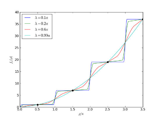
Figure 14.5: The function $f_{\lambda}(\rho)$ for the above described magnetic field model. The flux conditions require the function to pass through the black dots. A quadratic function corresponds to a uniform field while a staircase function corresponds to delta-function flux tubes. The parameter $\lambda$ smoothly transitions between these two extremes. Each of these functions corresponds to a magnetic field profile in figure 14.2.

The profile function, $f_{\lambda}(\rho)$, is plotted in figure 14.5.

Results

Comparing Scalar and Fermionic Effective Actions

Because of the fermion problem of $\mathrm{WLN}$ (see section 13.3), the 1-loop effective action for the cylindrical flux tube lattice model could not be computed for the case of spinor $\mathrm{QED}$. The fermion problem does not affect the scalar case. So, we are confined to analyzing this model for $\mathrm{ScQED}$.

For isolated flux tubes, the decay of the magnetic field for large distances protects the calculations from the fermion problem (see section 13.3). Therefore, the effective action can be computed for both scalar and spinor $\mathrm{QED}$. In figure 14.6, we plot the ratio of the spinor to scalar 1-loop correction term for identical magnetic fields, along with the prediction of the $\mathrm{LCF}$ approximation for large values of $\lambda$. The $\mathrm{LCF}$ approximation in $\mathrm{ScQED}$ is given by

$$\Gamma^{(1)}_{\rm scal} = -\frac{1}{2\pi}\int_{0}^{\infty}dT\int_{0}^{\infty}\rho_{\rm cm}d\rho_{\rm cm}\frac{e^{-m^{2}T}}{T^{3}}$$ (14.43)

$$\left\{\frac{eB(\rho_{\rm cm})T}{\sinh{(eB(\rho_{\rm cm})T)}}-1+\frac{1}{6}(eB(\rho_{\rm cm})T)^{2}\right\}.$$

This can be compared to the spinor $\mathrm{QED}$ approximation, equation (12.53).

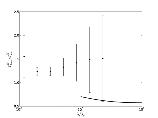
Figure 14.6: The ratio of the 1-loop term in $\mathrm{QED}$ to the 1-loop term in $\mathrm{ScQED}$. The solid line is the $\mathrm{LCF}$ approximation, while the points are the result of $\mathrm{WLN}$ calculations. Note that the $\mathrm{LCF}$ approximation breaks down near $\lambda=\lambda_{e}$ and that the statistics from point to point are strongly correlated. This plot shows that the 1-loop correction in $\mathrm{ScQED}$ differs from the $\mathrm{QED}$ correction by a factor close to unity for a wide range of flux tube widths.

There are two important notes to make about figure 14.6. Firstly, the $\mathrm{LCF}$ approximation is only a good approximation for $\lambda\gg\lambda_{e}$, and isn’t accurate when pushed near its formal validity limits [144]. The second note is that the statistics of the $\mathrm{WLN}$ points are strongly correlated. So, we conclude that the $\mathrm{ScQED}$ 1-loop correction is larger than the $\mathrm{QED}$ correction for large $\lambda$, and this appears to be reversed for small $\lambda$. However, the large $\mathrm{WLN}$ error bars and the invalidity of the $\mathrm{LCF}$ approximation near $\lambda=\lambda_{e}$ prevent us from seeing how this transition happens. Nevertheless, the main conclusion from this figure is that the scalar 1-loop correction reflects the behaviour of the full $\mathrm{QED}$ 1-loop correction to within a factor of about 2 over a wide range of flux tube widths for isolated flux tubes.

Besides using a finite field profile, the fermion problem can also be circumvented by increasing the electron mass. From equation (12.15), we can see that the square of the electron mass sets the scale for the exponential suppression of the large proper time Wilson loops that contribute to the fermion problem. However, if we increase the fermion mass, we are reducing the Compton wavelength of our theory so that the flux tube lattice is no longer dense in terms of the (new) Compton wavelength. It is the Compton wavelength of the theory that determines what is meant by ‘dense’. We therefore cannot avoid the fermion problem for dense lattice models by changing the electron mass.

Based on the results presented in figure 14.6, we conclude that the coupling between the electron’s spin and the magnetic field do not have a dramatic effect on the vacuum energy for isolated flux tubes. Therefore, we expect that $\mathrm{ScQED}$ provides a good model of the underlying vacuum physics near these flux tubes, at least at the level our toy model flux tube lattice.

Flux Tube Lattice

The $\mathrm{WLN}$ technique computes an effective action density which is then integrated to obtain the effective action. This quantity differs from the Lagrangian in that it is not determined by local operators, but encodes information about the field everywhere through the worldline loops. Like the classical action, the 1-loop term of the effective action per unit length is infinite for a flux tube lattice because the field extends infinitely far. For this reason, we define the effective action to be the action density integrated over the region of a central flux tube $(0<\rho<a/2)$:

$$\frac{\Gamma}{\mathcal{T}L_{z}} = -\pi\int_{0}^{a/2}\rho B_{z}(\rho)^{2}d\rho$$ (14.44)

$$-\frac{1}{2\pi}\int_{0}^{a/2}\rho_{\rm cm}d\rho_{\rm cm}\int_{0}^{\infty}\frac{dT}{T^{3}}e^{-m^{2}T}$$

$$\times\left\{\langle W\rangle_{\rho_{\rm cm}}-1+\frac{1}{6}(eB(\rho_{\rm cm})T)^{2}\right\}.$$

The 1-loop term of the effective action density is plotted in figure 14.7 for the cylindrical flux tube lattice model. The most pronounced feature of this density is that there is a negative contribution from the regions where the field is strong. This contribution has the same sign as the classical term. Therefore, quantum correction tends to reinforce the classical action. A less pronounced feature is that there is a positive contribution arising from the $\rho>\lambda/2$ region, in between the lumps of magnetic field which represent the flux tubes. In this region, the local magnetic field is positive, but small.

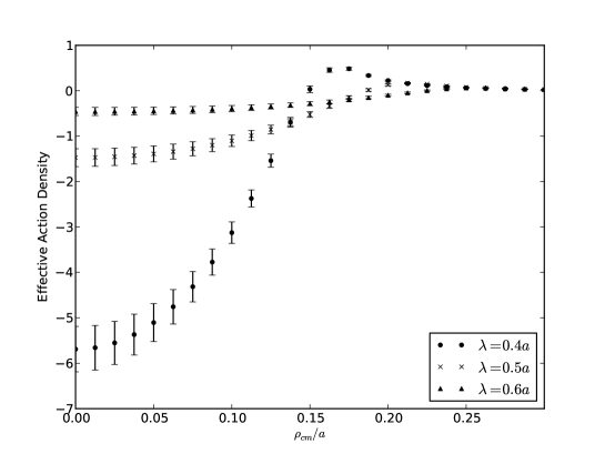
Figure 14.7: The $\mathrm{ScQED}$ effective action density for the central flux tube in our cylindrical lattice model for several tube widths, $\lambda$. The average field strength is the critical field, $B_{K}$. The effective action is positive in between flux tubes due to nonlocal effects.

To interpret this feature, we consider the relative contributions between the Wilson loops and the counter term. These terms are shown in figure 14.8 for the constant field case. For all values of proper time, $T$, the counter terms dominate, giving an overall negative sign. In order for the action density to be positive, there must be a greater contribution from the Wilson loop average than from the counter term, since this term tends to give a positive contribution to the action. In our flux tube model, this seems to occur in the regions between the flux tubes. In these regions, the local contribution from the counter term is relatively small because the field is small. However, the contribution from the Wilson loop average is large because the loop cloud is exploring the nearby regions where the field is much larger. The effect is largest where the field is small, but becomes large in a nearby region. We therefore interpret the positive contributions to the 1-loop correction from these regions as a non-local effect. A similar example of such an effect from fields which vary on scales of the Compton wavelength has been observed previously using the $\mathrm{WLN}$ technique [58].

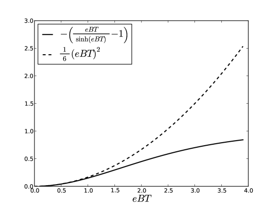
Figure 14.8: The Wilson loop and counter term contributions to the integrand of the effective action for a constant field in $\mathrm{ScQED}$. For constant fields, the effective action is always negative due to the domination of the counter term over the Wilson loop. For non-homogeneous fields, A positive effective action density signifies that non-local (i.e. $T>0$) effects dominate the counter term.

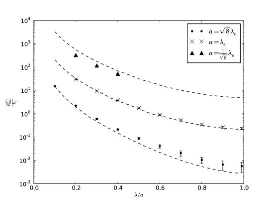
Figure 14.9: The 1-loop $\mathrm{ScQED}$ term of the effective action as a function of flux tube width, $\lambda/a$, for several values of the flux tube spacing, $a$. The dotted lines are computed from the $\mathrm{LCF}$ approximation.

In figure 14.9, we plot the magnitude of the 1-loop $\mathrm{ScQED}$ term of the effective action as a function of the flux tube width. As the flux tubes become smaller, there is an amplification of the 1-loop term, just as there is for the classical action. Similarly, for more closely spaced flux tubes, $a$ is smaller, and the 1-loop term increases in magnitude. The ratio of the 1-loop term to the classical term is plotted in figure 14.12. The quantum contribution is greatest for closely spaced, narrow flux tubes, but does not appear to become a significant fraction of the total action.

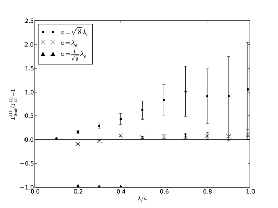
Figure 14.10: The residuals between the $\mathrm{WLN}$ results and the $\mathrm{LCF}$ approximation for the cylindrical flux tube lattice. The level of agreement is not expected because the field varies rapidly on the Compton wavelength scale. This agreement is believed to be due to an averaging effect of integrating over the electron degrees of freedom making a mean-field approximation appropriate.

We observe that the $\mathrm{LCF}$ approximation is surprisingly good despite the fact that the magnetic field is varying rapidly on the Compton wavelength scale of the electron. We plot the residuals showing the deviations between the $\mathrm{WLN}$ results and the $\mathrm{LCF}$ approximation in figure 14.10. To understand this, recall the discussion surrounding figure 14.8. The Wilson loop term is sensitive to the average magnetic field through the loop ensemble, $\langle B\rangle_{\rm e}$. In contrast, the counter term is sensitive to the magnetic field at the center of mass of the loop, $B_{\rm cm}$. Since these terms carry opposite signs, we can understand the difference from the constant field approximation in terms of a competition between these terms. When $B_{\rm cm}<\langle B\rangle_{\rm e}$, such as when the center of mass is in a local minimum of the field, there is a reduction of the energy relative to the locally constant field case, with a possibility of the quantum term of the energy density becoming negative. However, when $B_{\rm cm}>\langle B\rangle_{\rm e}$, such as in a local maximum of the field, there is an amplification of the energy relative to the constant field case. We can put a bound on the difference between the mean field through a loop and the field at the center of mass for small loops (i.e. small $T$),

$$|\langle B\rangle-B_{\rm cm}|\stackrel{{\scriptstyle<}}{{\sim}}|B^{\prime\prime}(\rho_{0})|T$$ (14.45)

where $|B^{\prime\prime}(\rho_{0})|\geq B^{\prime\prime}(\rho)$ for all $\rho$ in the loop. This expression is proved the same way as determining the error in numerical integration using the midpoint rectangle rule.

If the field varies rapidly about some mean value on the Compton wavelength scale, the various contributions from local minima and local maxima are averaged out and the mean field approximation provided by the $\mathrm{LCF}$ method becomes appropriate. A similar argument applies in the fermion case, where the important quantity is the mean magnetic field along the circumference of the loop. This quantity is also well served by a mean-field approximation when integrating over rapidly varying fields.

Another interesting feature of figure 14.10 is that the $\mathrm{LCF}$ approximation appears to describe narrower flux tubes better than wider ones, even when the spacing between the flux tubes is held constant. This effect is likely a result of the compact support given to the flux tube profiles. For narrow tubes, we are guaranteed to have many more center of mass points outside the flux tube than inside, giving a smaller energy contribution than for isolated flux tubes without compact support where the distinction between inside and outside is not as abrupt. This also explains why narrow, closely spaced tubes produce a lower energy than is predicted by the $\mathrm{LCF}$ approximation.

This argument does not apply to the smooth isolated flux tubes given by equation (14.6). For these flux tubes, the only region where there is a large discrepancy between $\langle B\rangle_{\rm e}$ and $B_{\rm cm}$ is near the center of the flux tube. This is a global maximum of the field, and the only maximum of $|B^{\prime\prime}(\rho)|$. There are no regions where the average field in the loop ensemble is much stronger than the center of mass magnetic field. So, we expect an amplification of the energy near the flux tube relative to the constant field case. In the flux tubes with compact support, however, there is such a region just outside the flux tube. We can understand the surprisingly close agreement of these results to the $\mathrm{LCF}$ approximation in our model in terms of competition between these regions of local minima and maxima of the field (see figure 14.11).

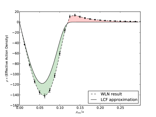
Figure 14.11: The action density in $\mathrm{WLN}$ and the $\mathrm{LCF}$ approximation, scaled by $\rho$ so an area on the figure is proportional to a volume. The approximation is poor everywhere, however, when there are regions of local minima and local maxima of the field about a mean value, the effective action approximately agrees between these methods. This is due to a partial cancellation between regions where the estimate provided by the approximation is too large (green) and other regions where the estimate is too small (red).

Finally, I find that the quantum term remains small compared to the classical action for the range of parameters investigated. This is shown in figure 14.12 where we plot the ratio of the $\mathrm{ScQED}$ term of the action to the classical action. The relative smallness of this correction is consistent with the predictions from homogeneous fields and the derivative expansion, as well as with previous studies on flux tube configurations [15].

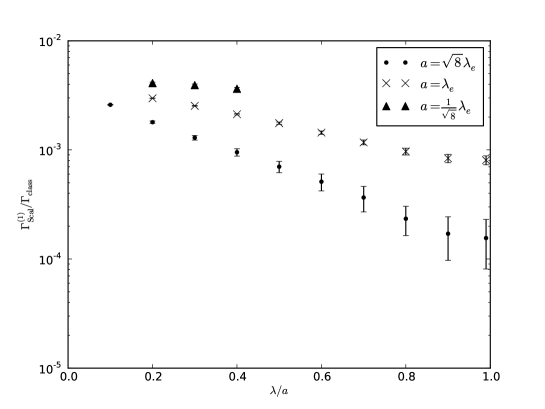
Figure 14.12: The 1-loop $\mathrm{ScQED}$ term divided by the classical term of the effective action as a function of flux tube width, $\lambda/a$ for several values of the flux tube spacing, $a$.

Interaction Energies

Using this model, we may also investigate the energy associated with interactions between the flux tubes. Since the flux tubes in our model exhibit compact support, the interaction energy is entirely due to a nonlocal interaction between nearby flux tubes. Thus, it contrasts with previous research which has investigated the interaction energies between flux tubes which have overlapping fields [114]. In this case, there is a classical interaction energy ($\propto B_{1}B_{2}$) as well as a quantum correction ($\propto(B_{1}+B_{2})^{4}-B_{1}^{4}-B_{2}^{4}$ in the weak-field limit). Even when these field overlap interactions are not present, there are also nonlocal energies in the vicinity of a flux tube due to the presence of other flux tubes. For example, the energy from nearby flux tubes can interact with a flux tube through the quantum diffusion of the magnetic field. Because of this phenomenon, we expect an interaction energy in the region of the central flux tubes due to the proximity of neighbouring flux tubes, even though no changes are made to the field profile or its derivatives in the region of interest. Since this interaction represents a force due to quantum fluctuations under the influence of external conditions, it is an example of a Casimir force. The Casimir force between two infinitely thin flux tubes in $\mathrm{ScQED}$ has previously been found to be attractive [43]. Our model can shed light specifically on this interaction, which is not predicted by local approximations such as the derivative expansion.

Consider a central flux tube with a width $\lambda=0.5\lambda_{e}$. When $\lambda_{\rm min}=\lambda$, the magnetic field outside of the flux tube, $B_{\rm bg}$, is zero. Then, if the distance between flux tubes, $a$, is set very large, the energy density will be localized to the central flux tube and there will be no nonlocal interaction energy due to neighbouring flux tubes. We define the interaction energy, $E_{\rm int}$, as the difference in energy within a distance $a/2$ of the central flux tube between a configuration with a given value of $a$ and a configuration with $a=\infty$. In practice, we use $a=10,000\lambda_{e}$ as a suitable stand-in for $a=\infty$:

$$\frac{E_{\rm int}}{L_{z}}=-\frac{\Gamma_{\rm scal}(a)}{L_{z}\mathcal{T}}+\frac{\Gamma_{\rm scal}(a=1\times 10^{4}\lambda_{e})}{L_{z}\mathcal{T}}.$$ (14.46)

With this definition, the interaction energy is the energy associated with lowering the distance between flux rings from infinity. This the the analogue in our model of reducing the lattice spacing of the flux tubes.

One complication of this definition is that there is no clear distinction between energy density which ‘belongs’ to the central flux tube and energy density which ‘belongs’ to the neighbouring flux tubes. We continue to use our convention that the total energy for the central flux tube is determined by the integral over the non-local action density in a region within a radius of $a/2$ of the flux tube. As $a$ is taken smaller and smaller, some energy from nearby flux tubes is included within this region, but also, some energy associated with the central flux tube is diffused out of the region. This ambiguity is unavoidable within this model. We can’t numerically compute the energy over all of space and subtract off different contributions, because these energies are infinite.

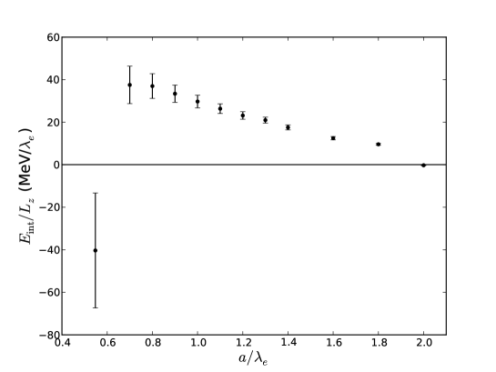
Figure 14.13: The interaction energy per unit length of flux tube as a function of the flux tube spacing, $a$. The energy density of a critical strength magnetic field is 17 GeV/$\lambda_{e}^{3}$, so this energy density is small in comparison to the classical magnetic field energies, or the 1-loop corrections. However, the local interactions are constant in $a$. At $a<\lambda_{e}/2$, the bump functions from neighbouring tubes overlap. This approximately corresponds to the critical magnetic field which destroys superconductivity.

The interaction energy is plotted in figure 14.13. In this plot, the error bars are 1-sigma error bars that account for the correlations in the means computed for each group of worldlines,

$$\sigma_{E_{\rm int}}=\sqrt{\sigma_{E_{a}}^{2}+\sigma_{E_{a=10000}}^{2}-2\operatorname{Cov}(E_{a},E_{a=10000})},$$ (14.47)

where $\operatorname{Cov}(a,b)$ is the covariance between random variables $a$ and $b$. Recall from figure 14.7 that there is a positive contribution to the effective action, and therefore a negative contribution to the energy from the region between flux tubes. As we reduce $a$, bringing the flux tubes closer together, two considerations become important. Firstly, we are increasing the average field strength meaning there tends to be more flux through the worldline loops which tends to give a negative contribution to the interaction energy. Secondly, we are reducing the spatial volume over which we integrate the energy since we only integrate $\rho$ from $0$ to $a/2$. This effect makes a positive contribution to the interaction energy since we include less and less of the region of negative energy density in our integral.

In figure 14.13, there appears to be a landscape with both positive and negative interaction energies at different values of $a$. These appear to be consistent with the interplay between positive and negative contributions described in the previous paragraph. This is consistent with the usual expectation of attractive Casimir forces [43]. The dominant contribution for the positive energy values is caused by less of the negative energy region contributing as the domain assigned to the flux tube is reduced. However, the point at $a/\lambda_{e}=2$ is negative ($-0.3\pm 0.1$MeV/$\lambda_{e}$) indicating that an attractive interaction from nearby flux tubes is dominant. We are continuing to compute points at larger values of $a$.

At $a/\lambda_{e}=0.5$, the flux tubes are positioned right next to one another, and the negative contribution from the increase in the mean field appears to be slightly larger than the positive contribution from the loss of the region of negative energy density from the integral. Beyond this, the flux tubes would overlap each other, which approximately corresponds to the critical background field which destroys superconductivity.

Based on the above explanation, it appears that the non-local interaction energy between magnetic fields has a strong dependence on the specific profile of the classical magnetic field that was used. This makes it difficult to predict if it will result in attractive or repulsive forces in a more realistic model of a flux tube lattice.

The energy density of a critical strength magnetic field is about $17{\rm GeV}/\lambda_{e}^{3}$, so the energy associated with this interaction is relatively small. However, there are no other interactions which affect the energy of moving the flux tubes closer together when they are separated by many coherence lengths. Here, the characteristic distance associated with the interaction, $\lambda_{e}$, is considerably larger than coherence length or London penetration depth, so the interactions between flux tubes through the order field are heavily suppressed.

Discussion and Conclusions

In this chapter, I have developed a cylindrically symmetric magnetic field model which reproduces some of the features of a flux tube lattice: for a given central flux tube, there are nearby regions of large magnetic field which interact nonlocally, and the large flux tube size limit goes to a large uniform magnetic field instead of to zero field. I have investigated the 1-loop effects from $\mathrm{ScQED}$ in this model using the $\mathrm{WLN}$ technique for various combinations of flux tube size, $\lambda$, and flux tube spacing, $a$.

In contrast to isolated flux tubes, I find that there are some regions where the $\mathrm{WLN}$ results are greater than the $\mathrm{LCF}$ approximation and other regions where they are less than the $\mathrm{LCF}$ approximation. This can be understood by thinking of the difference from the $\mathrm{LCF}$ approximation as a competition between the local counter term and the Wilson loop averages. For magnetic fields which vary on the Compton wavelength scale about some mean field strength, the $\mathrm{LCF}$ approximation provides a poor approximation of the energy density, but may provide a good approximation to the total energy density of the field due to it being a good mean field theory approximation to the energy density. The appropriateness of the $\mathrm{LCF}$ approximation in this case can be understood as an approximate balance between regions where the field is a local maximum and the magnitude of the quantum correction to the action density is larger than in the constant field case, and regions where the field is a local minimum and the quantum corrections predict a smaller action density than the constant field case. This washing out of the field structure due to non-local effects has also been observed in $\mathrm{WLN}$ studies of the vacuum polarization tensor [58].

There is a force between nearby magnetic flux tubes due to the quantum diffusion of the energy density. This interaction is non-local and is not predicted by the local derivative expansion. It is an example of a Casimir force (i.e. a force resulting from quantum vacuum fluctuations) and it is computed in a very similar way as the Casimir force between conducting bodies in the $\mathrm{WLN}$ technique [59]. The size of the energy densities involved in this force are small even compared to the 1-loop corrections to the energy densities, which are in turn small compared to the classical magnetic energy density.

Although this interaction energy is small, the interactions between flux tubes in a neutron star due to the order field of the superconductor are suppressed because the distance between the tubes is considerably larger than the coherence length and London penetration depth. Therefore, this force is possibly important for the behaviour of flux tubes in neutron star crusts and interiors. For example, in our lattice model, this force could contribute to a bunching of the worldlines, producing regions where flux tubes are separated by $\sim 2\lambda_{e}$ and other regions which have no flux tubes. Consequently, this force may have important implications for neutron star physics. However, investigating these implications is outside the scope of this thesis.

The nature of this interaction energy is expected to depend on the model of the magnetic field profile for the reasons discussed in section 14.4. It is therefore reasonable that forces of either sign, attractive or repulsive, may be possible depending on the particular landscape formed by the magnetic field and the particular definition used of the interaction energy. In a superconductor, the profiles of the magnetic flux tubes are determined by the minimization of the free energy for the interacting system formed by the magnetic and order parameter fields. Therefore, investigating this phenomenon using more realistic models is an interesting direction for future research. In particular, it would be interesting to determine if certain conditions allowed for a non-local interaction between magnetic flux tubes to be experimentally observable.

The conclusions from this chapter are applicable to $\mathrm{ScQED}$. However, we have also investigated the relationship between spinor and scalar $\mathrm{QED}$ for isolated flux tubes where the $\mathrm{WLN}$ technique can be applied to both cases. We find that both theories have the same qualitative behaviour, and agree within a factor of order unity quantitatively. The arguments and explanations given for the $\mathrm{ScQED}$ results have strong parallels in the spinor $\mathrm{QED}$ case. The spinor case can also be understood in terms of a competition between the Wilson loop averages and the local counter term. We therefore speculate that the results from this chapter will hold in the spinor case, at least qualitatively. However, addressing the fermion problem so that the spinor case can be studied explicitly for flux tube lattices would be valuable progress in this area of research.

Part IV Conclusions

Chapter 15 Conclusions

The goal of this dissertation has been to explore the role played by the quantum vacuum in extreme astrophysical environments. Specifically, we have explored three specific physical scenarios: (Part I) the generation of particles (and ultimately large-scale structure) during the universe’s inflationary epoch, (Part II) the propagation of strong electromagnetic waves through the magnetosphere of a magnetar, and (Part III) densely packed flux tubes inside the nuclear matter in a pulsar. In each case, I developed models of quantum field theories coupled non-perturbatively to their environment and used these models to explore the possible role that the quantum vacuum might play in these astrophysical systems. This research has produced new insights into the physics of both the quantum vacuum and of the astrophysical scenarios studied. Additionally, this dissertation also makes contributions to the methods available for studying quantum field theories under external conditions. In this conclusion, we will review the main scientific contributions of this dissertation, and suggest some possible directions for future research which could draw on this work.

Inflation

In chapter 7, we generalized a particle picture of quantum fluctuations during inflation to include the effects of nonlinear interactions. Thus, we were able to simulate the quantum mechanical evolution of the field treating both the gravitational interaction and the self-interaction nonperturbatively. This model was useful for tracking exactly the entanglement entropy between modes. This new insight allowed us to make a comparison between the entanglement entropy and other measures of decoherence used in the literature. Decoherence arising from non-linear interactions is not efficient enough to explain classicality in general, but it leaves open the exciting possibility that scalar fields not participating in reheating may keep some quantum characteristics that may some day be measurable. It is possible that the techniques of the particle picture developed for this dissertation may be applicable to studying entanglement entropy in other systems.

One possible example is to use the particle picture to address the apparent loss of information from evaporating black holes (i.e. the information loss problem). The final state of an evaporated black hole is expected to be described by a mixed, thermal density matrix, even in the case where the initial state was a pure state [185]. This evolution from a pure state to a mixed state is impossible in a closed system through unitary evolution, according to the postulates of quantum mechanics. It has been shown that the entanglement entropy of scalar fields in their ground state near the black hole horizon can reproduce the form of the Beckenstein-Hawking entropy [13, 178]. This provides a hint that the black hole entropy may be due to quantum mechanical degrees of freedom. This idea has led to recent interest in investigating the von Neumann entropy contained in scalar fields near the black hole’s horizon, tracing over the region which is inaccessible due to the horizon [35, 19]. The degrees of freedom from such a field give an entanglement entropy to the system, and have been shown to lead to corrections to the Beckenstein-Hawking entropy in certain circumstances [36]. Therefore, one expects that by studying the black hole spacetime in a conformally flat Euclidean path-integral formalism, a Schrödinger-like equation will emerge describing the unitary evolution of quantum states, but with an entanglement entropy consistent with the Beckenstein-Hawking entropy due to entanglement between modes inside and outside of the horizon. So, the particle picture may provide a new way of looking at black hole information loss, and may bring new insights to the problem.

Another potential application of the particle picture is simulating the quantum coherence of relic neutrinos. Neutrinos have the interesting property that their mass eigenstates are not coincident with their flavour eigenstates [143]. One of the consequences of this is that the flavour eigenstates of the cosmological relic neutrino background become spread out to very large cosmological scales because they are in a superposition of different mass states which travel at different speeds and become nonrelativistic at different cosmological epochs. It is possible then that a flavour eigenstate can be in a large-scale coherent superposition of relativistic and nonrelativistic mass states at the epoch when neutrinos begin to collapse into dark matter gravitational wells. So, this leads to the question of whether gravitational tidal stresses can lead to decoherence between the mass eigenstates of relic neutrinos [50]. It may be possible to use the particle picture methods to address decoherence in this scenario.

Electromagnetic Waves Near a Magnetar

In chapter 9, I developed a computational method for searching for travelling wave solutions to the 1-loop $\mathrm{QED}$ corrected Maxwell’s equations in a plasma. This tool has uncovered a new class of waves which form long wave chains with highly non-sinusoidal profiles. These waves may have an effect on energy transport near neutron stars which may have observable implications for pulsar microstructure. So, incorporating this phenomenon into a holistic model of the pulsar magnetosphere and determining if it results in observable predictions is a future step in this line of research.

One weakness of the findings from this section is that the travelling wave conditions were assumed a priori. So, while the results demonstrate that the stable travelling waves are a possible outcome for electromagnetic waves coupled to a plasma, it is not possible to tell from the analysis if they are a likely outcome compared to waves which form shocks. So, determining what conditions will produce waves which are stable compared to ones that collapse is an interesting problem which follows from this research.

This study used a relatively simple plasma model consisting of a relativistic pair plasma at zero temperature. This model is appropriate considering the intense magnetic fields involved. However, it is straightforward to extend the model to more detailed or realistic plasma models. Typically, these can be incorporated by modifying the vacuum dielectric and permeability tensors appropriately to account for a multi-species plasma, non-linearities, and/or thermal effects.

One of the original motivations for developing the methods for this study was to explore the possibility that solitons may be formed in the $\mathrm{QED}$ vacuum + plasma system. These solutions would represent stable bundles of electromagnetic energy that would travel through the magnetosphere, and a novel structure of the $\mathrm{QED}$ quantum vacuum coupled to a plasma. While no solitonic waves have yet been discovered in such a system, this remains a possible application for the techniques that can be further explored in the future.

Flux tubes

In general, evaluating the fermion determinants in non-homogeneous fields is a challenging problem without many techniques and approaches available to researchers. Through my investigations of $\mathrm{QED}$ magnetic flux tubes, I have derived a new expression for the effective action of cylindrically symmetric magnetic fields based on a Green’s function technique which is suitable for numerical calculations. This technique is the subject of chapter 11. While the expressions derived in this section are difficult to work with and were not ultimately employed, they may prove useful for future research into the effective actions of flux tube configurations. An interesting result from this line of research is that an expression can be derived which extremizes the effective action with respect to the function that describes the magnetic field profile. This expression includes contributions from $\mathrm{QED}$ which suggests that some nonhomogeneous magnetic field extremizes the effective action in contrast to the purely classical case. This result begs the question of what effect the quantum corrections have to the stability of flux tubes and flux tube lattices.

In order to compute the effective actions of flux tubes, I ultimately turned to the numerical worldline (or loop cloud) method. Two contributions to this technique are made in this dissertation and are discussed in chapters 12 and 13. Firstly, I made the observation that the non-Gaussian nature of the worldline distributions and the correlations between the computed points in the integrals should both be taken into account in the uncertainty analysis. Chapter 13 is the first thorough discussion of error analysis for the $\mathrm{WLN}$ technique. Such a discussion is important because the subtleties can be easily missed or ignored by new adopters of the technique. Secondly, by implementing the technique on $\mathrm{GPU}$s, I have been able to achieve a 3600-fold speed increase over a serial implementation in computing Wilson loop averages. This likely makes my implementation of the Wilson loop algorithm an order of magnitude faster than a parallel implementation on $\mathrm{CPU}$ clusters with hundreds of processors and demonstrates that the $\mathrm{GPU}$s architecture is very well suited to the technique. Dramatic speed increases in computational physics such as this may open up entirely new avenues of research. Since the worldline numerical technique has been useful in a variety of applications, developing the technique for $\mathrm{GPU}$ may help research in computing effective actions, Casimir energies [59, 145], or problems in $\mathrm{QCD}$.

Further development of the $\mathrm{WLN}$ code could produce increased performance, robustness, and greater flexibility in terms of the types of scenarios which could be computed. For example, more highly developed integration software such as that provided by $\mathrm{GSL}$, would improve the robustness and reliability of the code. These libraries cannot be used directly for $\mathrm{GPU}$ device code, but would be simple to implement for the integrals over proper time and centre of mass which are currently computed by the $\mathrm{CPU}$. The most significant performance bottleneck in the algorithm is the large portion of the computation which is performed serially. Parallelizing parts of this serial portion with additional $\mathrm{CUDA}$ kernels would help to accelerate the algorithm. There an opportunity for this kind of optimization, but this can only be done for portions of code which do not depend on the Wilson loop kernel. One could also straightforwardly parallelize the algorithm onto several $\mathrm{GPU}$ devices, with each one responsible for a different centre of mass point, for example. Finally, there is also some room for optimizing the memory throughput to accelerate the Wilson loop calculations themselves for kernels which can make frequent use of the fast shared memory, or for $\mathrm{GPU}$s which can store the worldline data in constant memory.

In chapter 14, I have developed a cylindrically symmetric toy model intended to reproduce some aspects of a triangular lattice of flux tubes. I have used this model, and the worldline numerics technique to compute the $\mathrm{ScQED}$ effective action of a flux tube in a situation where nonlocal effects are expected to be significant. The quantum corrections to the energies in these configurations are small and are close to the $\mathrm{LCF}$ approximation because the energy density is diffused by the worldline loops so that the total energy is close to the mean field approximation. Nevertheless, I find that there is a nonlocal interaction between flux tubes which is not predicted by local techniques such as a derivative expansion. While the Casimir force between two infinitely thin solenoids has been previously computed [43], the $\mathrm{WLN}$ technique opens up the possibility of exploring this force for other less idealized field configurations.

Although this interaction is generally small, it occurs between flux tubes separated by a Compton wavelength, while the distance scales associated with flux tube interactions in a neutron star are typically much smaller. Therefore, if the flux tube density is such that the distance between tubes is comparable to a Compton wavelength, this interaction may have a considerable impact on the of the flux tubes. If this force is attractive at distances much greater than the coherence length and London penetration depths, it may contribute to a bunching of flux tubes. Investigating the consequences of this force for neutron star physics, and possibly for laboratory experiments is a very interesting goal for future research.

The $\mathrm{WLN}$ technique does not require any special symmetries, so it is easily generalizable to a more realistic flux tube lattice geometry. However, this would be significantly more computationally expensive because there is an additional spatial dimension to integrate, and more worldlines consisting of more points per line may be required. We were not able to compute effective actions for fermionic $\mathrm{QED}$ because of the fermion problem: when the fields are not well localized, one must compute the ratio of two very large numbers which results in amplified uncertainties. Future research should focus on addressing this problem so that the worldline technique can be applied to lattice configurations, which have large magnetic fields distributed throughout space.

A very compelling prediction of $\mathrm{QFTs}$ is that the laws of physics are played out on a lively background called the quantum vacuum. In this thesis, I have developed new physical models designed to illuminate specific aspects of how this quantum vacuum influences three different astrophysical scenarios: the emergence of classicality in the large scale structure of the universe, the behaviour of travelling electromagnetic waves near a magnetar, and the energies of narrow, densely spaced flux tubes in a superconducting neutron star. For each of these scenarios, I have performed novel mathematical and numerical analyses which have lead to contributions to the tools available to physicists, and to new physical insights about the systems studied. This thesis has contributed to our understanding of the interesting relationships which can exist between the vacuum and extreme astrophysical objects. Understanding these relationships is critical for understanding these objects in detail, and is also crucial to learning how observing these objects can contribute to our knowledge of the microscopic physics of the quantum vacuum.

Appendix A $\mathrm{CUDA}$fication of Worldline Numerics

My implementation of the $\mathrm{WLN}$ technique used a “co-processing” (or heterogeneous) approach where the $\mathrm{CPU}$ and $\mathrm{GPU}$ are both used in unison to compute different aspects of the problem. The $\mathrm{CPU}$ was used for computing the spatial and proper-time integrals while the $\mathrm{GPU}$ was employed to compute the contributions to the Wilson Loop from each worldline in parallel for each value of $\rho_{\rm cm}$ and $T$. This meant that each time the integrand was to be computed, it could be computed thousands of times faster than on a serial implementation. A diagram illustrating the co-processing approach is shown in figure 12.3

Code which runs on the $\mathrm{GPU}$ device must be implemented in the $\mathrm{CUDA}$-C programming language [151, 149]. The $\mathrm{CUDA}$ language is an extension of the C programming language and compiles under a proprietary compiler, nvcc, which is based off of the $\mathrm{GNU}$ C compiler, gcc.

Overview of $\mathrm{CUDA}$

$\mathrm{CUDA}$ programs make use of special functions, called kernel functions, which are executed many times in parallel. Each parallel thread executes a copy of the kernel function, and is provided with a unique identification number, threadIdx. threadIdx may be a one, two, or three-dimensional vector index, allowing the programmer to organize the threads logically according to the task.

A program may require many thousands of threads, which are organized into a series of organizational units called blocks. For example, the Tesla C1060 $\mathrm{GPU}$ allows for up to 1024 threads per block. These blocks are further organized into a one or two-dimensional structure called the grid. $\mathrm{CUDA}$ allows for communication between threads within a block, but each block is required to execute independently of other blocks.

$\mathrm{CUDA}$ uses a programming model in which the $\mathrm{GPU}$ and $\mathrm{CPU}$ share processing responsibilities. The $\mathrm{CPU}$ runs a host process which may call different kernel functions many times over during its lifetime. When the host process encounters a kernel function call, the $\mathrm{CUDA}$ device takes control of the processing by spawning the designated number of threads and blocks to evaluate the kernel function many times in parallel. After the kernel function has executed, control is returned to the host process which may then copy the data from the device to use in further computations.

The $\mathrm{GPU}$ device has separate memory from that used by the $\mathrm{CPU}$. In general, data must be copied onto the device before the kernel is executed and from the device after the kernel is executed. The $\mathrm{GPU}$ has a memory hierarchy containing several types of memory which can be utilized by threads. Each thread has access to a private local memory. A block of threads may all access a shared memory. Finally, there is memory that can be accessed by any thread. This includes global memory, constant memory, and texture memory. These last three are persistent across kernel launches, meaning that data can be copied to the global memory at the beginning of the program and it will remain there throughout the execution of the program.

Implementing $\mathrm{WLN}$ in $\mathrm{CUDA}$-C

In the jargon of parallel computing, an embarrassingly parallel problem is one that can be easily broken up into separate tasks that do not need to communicate with each other. The worldline technique is one example of such a problem: the individual contributions from each worldline can be computed separately, and do not depend on any information from other worldlines.

Because we may use the same ensemble of worldlines throughout the entire calculation, the worldlines can be copied into the device’s global memory at the beginning of the program. The global memory is persistent across all future calls to the kernel function. This helps to reduce overhead compared to parallelizing on a cluster where the worldline data would need to be copied many times for use by each $\mathrm{CPU}$. The memory copy can be done from $\mathrm{CPU}$ code using the built-in function cudaMemcpy() and the built-in flag cudaMemcpyHostToDevice.

⬇

//Copy worldlines to device

errorcode = cudaMemcpy(worldlines_d, worldlines_h,

nThreads*nBlocks*Nppl*sizeof(*worldlines_h),

cudaMemcpyHostToDevice);

if(errorcode > 0) printf(”cudaMemcpy WLs:

\%s\n”, cudaGetErrorString(errorcode));

The full source listing appears in appendix B.2. In the above, worldlines_d and worldlines_h are pointers of type float4 (discussed below) which point to the worldline data on the device and host, respectively. nThreads, nBlocks, and Nppl are integers representing the number of threads per block, the number of blocks, and the number of points per worldline. So, nThreads*nBlocks*Nppl*sizeof(*worldlines_h) is the total size of memory to be copied. The variable errorcode is of a built-in $\mathrm{CUDA}$ type, cudaError_t which returns an error message through the function cudaGetErrorString(errorcode).

The global memory of the device has a very slow bandwidth compared to other memory types available on the $\mathrm{CUDA}$ device. If the kernel must access the worldline data many times, copying the worldline data needed by the block of threads to the shared memory of that block will provide a performance increase. If the worldline data is not too large for the device’s constant memory, this can provide a performance boost as well since the constant memory is cached and optimized by the compiler. However, these memory optimizations are not used here because the worldline data is too large for constant memory and is not accessed many times by the kernel. This problem can also be overcome by generating the loops on-the-fly directly on the $\mathrm{GPU}$ device itself without storing the entire loop in memory [3].

In order to compute the worldline Wilson loops, we must create a kernel function which can be called from $\mathrm{CPU}$ code, but which can be run from the $\mathrm{GPU}$ device. Both must have access to the function, and this is communicated to the compiler with the $\mathrm{CUDA}$ function prefix __global__.

⬇

#define THREADS_PER_BLOCK 256

#if __CUDA_ARCH__ >= 200

#define MY_KERNEL_MAX_THREADS (2 * THREADS_PER_BLOCK)

#define MY_KERNEL_MIN_BLOCKS 3

#else

#define MY_KERNEL_MAX_THREADS (2 * THREADS_PER_BLOCK)

#define MY_KERNEL_MIN_BLOCKS 2

#endif

__global__ void

__launch_bounds__(MY_KERNEL_MAX_THREADS, MY_KERNEL_MIN_BLOCKS)

__global__ void ExpectValue(float4 *Wsscal, float4 *Wsferm,

float4 *worldlines, float4 xcm, float F,

float l2, float rtT, int Nl, int Nppl, int fermion)

//Each thread computes the Wilson loop value for a single

//worldline identified by inx.

{

int inx = blockIdx.x * blockDim.x + threadIdx.x;

WilsonLoop(worldlines, Wsscal, Wsferm,

xcm, inx, F, l2, rtT, Nppl, fermion);

}

The above listing is an excerpt from the file listed in appendix B.5. The preprocessor commands (i.e. the lines beginning with #) and the function __launch_bounds__() provide the compiler with information that helps it minimize the registers needed and prevents spilling of registers into much slower local memory. More information can be found in section B.19 of the $\mathrm{CUDA}$ programming guide [149]. The built-in variables blockIdx, blockDim, and threadIdx can be used as above to assign a unique index, inx, to each thread. $\mathrm{CUDA}$ contains a native vector data type called float4 which contains a four-component vector of data which can be copied between host and device memory very efficiently . This is clearly useful when storing coordinates for the worldline points or the center of mass. These coordinates are accessed using C’s usual structure notation: xcm.x, xcm.y, xcm.z, xcm.w. I also make use of this data type to organize the output Wilson loop data, Wsscal and Wsferm, into the groups discussed in section 13.1.

The function WilsonLoop() contains code which only the device needs access to, and this is denoted to the compiler by the __device__ function prefix. For example, from appendix B.5, we have,

⬇

extern ”C”

__device__ void WilsonLoop(float4 *worldlines, float4 *Wsscal,

float4 *Wsferm, float4 xcm, int inx, float F, float l2,

float rtT, int Nppl, int fermion)

//Compute the WilsonLoops for the thread inx and store the

//results in Wsscal[inx] (scalar part)

//and Wsferm[inx] (fermion part)

{

…

}

Note that we pass $\sqrt{T}$ to the function (float rtT) instead of $T$ so that we only compute the square root once instead of once per thread. Avoiding the square root is also why I chose to express the field profile in terms of $\rho^{2}$.

As mentioned above, the $\mathrm{CUDA}$ device is logically divided into groups of threads called blocks. The number of blocks, nBlocks, and the number of threads per block, nThreads, which are to be used must be specified when calling $\mathrm{CUDA}$ kernel functions using the triple angled bracket notation.

⬇

MyKernel<<<nBlocks,nThreads>>>(void* params)

In the following snippet of code, we call the $\mathrm{CUDA}$ device kernel, ExpectValue() from a normal C function. We then use the cudaMemcpy() function to copy the Wilson loop results stored as an array in device memory as params.Wsscal_d to the host memory with pointer params.Wsscal_h. The contents of this variable may then be used by the $\mathrm{CPU}$ using normal C code, as is done in appendix B.5.

⬇

//Call to CUDA device

ExpectValue<<<params.nBlocks, params.nThreads>>>(

params.Wsscal_d, params.Wsferm_d,

params.worldlines, params.xcm, params.F,

params.l2, rtT,params.Nl, params.Nppl

);

//Check for errors during kernel execution

errorcode = cudaGetLastError();

if (errorcode > 0) printf(

”cuda getLastError EV(): %s\n”,

cudaGetErrorString(errorcode)

);

//Copy device memory back to host

errorcode = cudaMemcpy(

params.Wsscal_h, params.Wsscal_d,

params.Nl*sizeof(params.Wsscal_h[0]),

cudaMemcpyDeviceToHost

);

//Check for memory copy errors

if(errorcode > 0) printf(

”CUDA memcpy scal Error EV(): %s\n”,

cudaGetErrorString(errorcode)

);

if(params.fermion == 1) //if fermionic calculation

{

//Copy fermion data from device to host

errorcode = cudaMemcpy(

params.Wsferm_h, params.Wsferm_d,

params.Nl*sizeof(params.Wsferm_h[0]),

cudaMemcpyDeviceToHost

);

//Check for memory copy errors

if(errorcode > 0) printf(

”CUDA memcpy ferm Error EV(): %s\n”,

cudaGetErrorString(errorcode)

);

};

Compiling $\mathrm{WLN}$ $\mathrm{CUDA}$ Code

Compilation of $\mathrm{CUDA}$ kernels is done through the Nvidia $\mathrm{CUDA}$ compiler driver nvcc. nvcc can be provided with a mixture of host and device code. It will compile the device code and send the host code to another compiler for processing. On Linux systems, this compiler is the $\mathrm{GNU}$ C compiler, gcc. In general, nvcc is designed to mimic the behaviour of gcc. So the interface and options will be familiar to those who have worked with gcc.

There are two dynamic libraries needed for compiling $\mathrm{CUDA}$ code. They are called libcuda.so and libcudart.so and are located in the $\mathrm{CUDA}$ toolkit install path. Linking with these libraries is handled by the nvcc options -lcuda and -lcudart. The directory containing the $\mathrm{CUDA}$ libraries must be referenced in the \$LD_LIBRARY_PATH environment variable, or the compiler will produce library not found errors.

Originally, $\mathrm{CUDA}$ devices did not support double precision floating point numbers. These were demoted to float. More recent devices do support double, however. This is indicated by the compute capability of the device being equal or greater than 1.3. This capability is turned off by default, and must be activated by supplying the compiler with the option -arch sm_13. The kernel presented in section B.5 primarily uses float variables because this reduces the demands on register memory and allows for greater occupancy.

Another useful compile option is –ptxas-options=”-v”. This option provides verbose information about shared memory, constants, and registers used by the device kernel. The kernel code for my project became sufficiently complex that I ran out of registers and suffered some baffling behaviour from the program that I wasn’t initially error checking for properly. This can be avoided by paying attention to the number of registers in use, and using the $\mathrm{CUDA}$ Occupancy Calculator spreadsheet provided by Nvidia to determine the maximum number of threads per block that can be supported [150]. However, the $\mathrm{CUDA}$ error checking used in this chapter is sufficient to discover the problem if it arises.

A Makefile showing the compilation and linking of a program defined by multiple .c, .cu and .h files is given in appendix B.7.

Appendix B $\mathrm{WLN}$ Source Code

In this appendix, I collect a listing of the source code used for the calculations in chapters 12, 13 and 14. To obtain compileable code, these listings can be copy and pasted, taking care to fix strings which have been split onto two lines, and removing page numbers.

• Section B.1 contains a header file used by many of the .c and .cu files.

• The main driver for the program and the routines for performing the integral over center of mass is listed in section B.2.

• The routines for integrating over proper time are listed in section B.3.

• The functions for computing the integrand of the proper time and center of mass integrals are provided in section B.4.

• Section B.5 contains the $\mathrm{CUDA}$ kernel and the $\mathrm{CUDA}$ device functions which compute the scalar and fermionic contributions to the Wilson loops.

• The routine for reading worldline data from an ASCII file is listed in section B.6.

• Section B.7 contains the Makefile which compiles software using the Nvidia proprietary compiler nvcc.

• Two Matlab functions which are used to generate worldline data and save them to ASCII files are listed in section B.8.

Common Header File - intT.h

A header file shared by all of the .c and .cu files.

⬇

struct Wparams

{

float4 *worldlines; //worldline points

float4 *Wsscal_d; //scalar Wilson exponents on device

float4 *Wsscal_h; // ” on host

float4 *Wsferm_d; //fermion Wilson exponents on device

float4 *Wsferm_h; // ” on host

float4 xcm; //center of mass of loop cloud

double F; //flux parameter

double l2; //radius squared of flux tube

int Nppl; //Number of points per line

int Nl; //Number of loops

int ng; //Number of groups for jackknife

int fermion; //Flag for scalar/spinor QED calculation

int nBlocks; //Number of blocks on cuda device

int nThreads; //Number of threads per CUDA block

double SE; //Standard Error

float *rho2sp; //rho^2 spline points for periodic field

float4 *flcoefs; //spline coefficients for periodic field

};

//Function prototypes

int getwl(float4 *worldlines, char *filename, int Nl,

int Nppl, int Dim);

__global__ void ExpectValue(float4 *Wsscal, float4 *Wsferm,

float4 *worldlines, float4 xcm, float F, float l2,

float rtT, int Nl, int Nppl, float4 *flcoefs,

float *rho2sp, int fermion);

double* integrateT(int n, double tmax, void * p);

double* Tfunc(double T, void* p, int* order);

//Constant definitions

#ifndef intT_h

#define intT_h

#define m2 1.0 //electron mass squared

#define e 0.302822121 //electron charge (alpha = e^2/(4 pi))

#define pi 3.14159265

#define verbosity 2 //determines amount of output

#endif

//Profile definitions and constants

#ifndef profile

enum proftype {

step,

smooth,

quadratic, //untested

gaussian,

periodic, //untested

spline, //untested

fixflux

};

//Select the profile here

enum proftype profile = smooth;

#define Nspline 10000 //for spline

#define tubedist 8.0 //for fixflux

#define q1 0.443991 //bump function const. for fixflux

#define q2 0.0742478 //bump function const.for fixflux

#define lmin (0.1f*tubedist) //for fixflux

#endif

intT.h

Main Program Driver - EffAct.c

Contains the main() function and routines for performing the integral over $\rho_{\rm cm}$.

⬇

#include <stdio.h>

#include <stdlib.h>

#include <math.h>

#include <builtin_types.h>

#include ”intT.h”

double MagField( double rho2, void* p );

float4* getspline( float* rho2, double lambda2,

double a, int Npoints );

double testspline( float rho2, double lambda2, double a,

int Npoints, float *rho2sp, float4 *flcoefs);

double* rhogrand(double rho, void* p)

//The Lagrangian Density Function

{

int i, Npoints = 100;

double *intout;

double tmax, Bcm;

struct Wparams *params = (struct Wparams *) p;

//by symmetry, we may integrate rho along the x-axis

params->xcm.x = rho;

params->xcm.y = 0.0;

params->xcm.z = 0.0;

//Determine the T value where the constant

//field integrand has a maximum for large fields

Bcm = MagField(rho*rho, p);

if (e*Bcm > 100.0)

tmax = 3.0/(e*Bcm); //from large field limit

else

tmax = 1.0;

//perform the proper time integration

if(verbosity >= 2)

printf(”Beginning T integration\n”);

//cudaSetDevice();

intout = integrateT(Npoints, tmax, p);

if(verbosity >= 2)

printf(”Returning from T integration\n”);

//for each group of worldlines

for(i = 0; i < params->ng; i++)

{

//multiply the integrand by rho

intout[i] = rho*intout[i];

}

return intout;

}

void testvalrho(double *val, int n, double t)

//Outputs diagnostic information about the rho integrand

{

int i;

double avg=0.0; //average

double SEM=0.0; //standard error in the mean

//compute the average

for(i = 0; i < n; i++)

{

if( isnan(val[i]) )

printf(”for rho=%f val[%d]=nan\n”,

(1.0-t)/t, i);

avg += val[i];

}

avg /= n;

//compute the standard error

for(i = 0; i < n; i++)

{

SEM += (val[i]-avg)*(val[i]-avg);

}

SEM = sqrt(SEM/((double)n*((double)n-1.0)));

//rho Leff SEM-Leff

printf(”testvalrho: %f %f %f\n”, (1.0-t)/t, avg, SEM);

}

double* transformRho(double rhot, void* p)

//Maps the interval [0,inf) to [0,1] using rho=(1-rhot)/rhot

{

struct Wparams *params = (struct Wparams *) p;

double* rhofunc;

double rho = (1.0-rhot)/rhot;

int i;

rhofunc = rhogrand(rho, p);

for(i = 0; i < params->ng; i++)

{

rhofunc[i] = (rhofunc[i]/rhot)/rhot;

}

return rhofunc;

}

double* integrateRhotoa(int n, void * p)

//integrates rho from 0 to a/2 for periodic flux tubes

//This algorithm is the composite Simpson’s rule as

//described in Burden and Faires ”Numerical Analysis”, 7th ed.

{

double* val;

double* XI0;

double* XI1;

double* XI2;

double* rg;

double* rg2;

struct Wparams *params = (struct Wparams *) p;

double rho;

int inx, ig, i;

val = (double *)calloc(params->ng, sizeof(*val));

XI0 = (double *)calloc(params->ng, sizeof(*XI0));

XI1 = (double *)calloc(params->ng, sizeof(*XI1));

XI2 = (double *)calloc(params->ng, sizeof(*XI2));

double h = tubedist/((double) 2*n);

double rhot;

if(!val) printf(”integrate(): malloc failed\n”);

rg = rhogrand(0.0, p);

rg2 = rhogrand(tubedist/2.0, p);

for(ig = 0; ig < params->ng; ig++)

{

val[ig] = 0.0;

XI1[ig] = 0.0;

XI2[ig] = 0.0;

XI0[ig] = rg[ig] + rg2[ig];

}

for(inx = 0; inx < n; inx++)

{

printf(”rho integrate inx=%d\n”, inx);

rho = h*((double)inx + 1.0);

rg = rhogrand(rho, p);

for(ig = 0; ig < params->ng; ig++)

{

if(inx%2 == 0) XI2[ig] += rg[ig];

else XI1[ig] += rg[ig];

}

free(rg);

}

for(ig = 0; ig < params->ng; ig++)

{

val[ig] = h/3.0*(XI0[ig] + 2.0*XI2[ig] + 4.0*XI1[ig]);

}

free(XI0); free(XI1); free(XI2); free(rg2);

return val;

}

double* integrateRho(int n, void * p)

//integrates rho from 0 to infinity for isolated flux tubes

//This algorithm is the composite Simpson’s rule as

//described in Burden and Faires ”Numerical Analysis”, 7th ed.

{

double* val;

double* rhort;

double* rhortphalf;

double* rhortp1;

struct Wparams *params = (struct Wparams *) p;

int inx, ig, i;

val=(double *)calloc(params->ng, sizeof(*val));

double h = 1.0/((double) n);

double rhot;

if(!val) printf(”integrate(): malloc failed\n”);

for(ig = 0; ig<params->ng; ig++)

{

val[ig] = 0.0;

}

for(inx = 0; inx < n; inx++)

{

printf(”rho integrate inx=%d\n”, inx);

rhot = h*((double)inx+1.0);

rhort = transformRho(rhot, p);

rhortphalf = transformRho(h*((double)inx + 0.5), p);

rhortp1 = transformRho(h*((double) inx+1.0), p);

for(ig = 0; ig < params->ng; ig++)

{

//check for infinities and nans

if(isinf(rhort[ig]))

{

printf(”Warning: rhort[%d]=%f.

Setting to zero.\n”, ig, rhort[ig]);

rhort[ig]=0.0;

}

if(isinf(rhortphalf[ig]))

{

printf(”Warning: rhortphalf[%d]=%f.

Setting to zero.\n”,ig,rhortphalf[ig]);

rhortphalf[ig]=0.0;

}

if(isinf(rhortp1[ig]))

{

printf(”Warning: rhortp1[%d]=%f.

Setting to zero.\n”,ig,rhortp1[ig]);

rhortp1[ig]=0.0;

}

//This equation extrapolates the three different

//Nppl spacings to Nppl=infinity

val[ig] += h/6.0*(

rhort[ig]

+ 4.0*rhortphalf[ig]

+rhortp1[ig]);

if(isinf(val[ig])){

printf(”rhort[%d]=%f\n”, ig, rhort[ig]);

printf(”rhortphalf[%d]=%f\n”, ig,

rhortphalf[ig]);

printf(”rhortp1[%d]=%f\n”, ig, rhortp1[ig]);

printf(”val[%d]=%f\n”, ig, val[ig]);

}

}

}

free(rhort);

free(rhortphalf);

free(rhortp1);

return val;

}

double PeriodicCA(double l2)

//Computes the spline Classical action

{

double a = tubedist;

double l = sqrt(l2);

double expal = exp(a/l);

double expalp1 = 1.0 + expal;

double PCA;

PCA = 2.0*a + 4.0*a/(expalp1*expalp1*expalp1)

-l + 4.0*l/expalp1

-2.0*(3.0*a+2.0*l)/(expalp1*expalp1)

+ l*log(16.0)-4.0*l*log(expalp1);

return PCA;

}

double FixFluxCA(double l2)

//Computes the fixflux (periodic) classical action

{

double q3 = 0.0187671;

double a = tubedist;

double l = sqrt(l2);

double A = q3*(a*a/(l2*q2*q2));

double lmlmin = (l-lmin)/(a-lmin);

double FFCA;

FFCA = 4.0*A + lmlmin*((9.0/4.0*A-9.0/2.0)*lmlmin

- 6.0*A + 12.0);

return FFCA;

}

double ClassAction(double F, double l2)

//Returns the Classical action for the given flux tube profile

{

double CA;

switch(profile){

case step:

CA=-2.0*pi*F*F/(e*e*l2);

break;

case smooth:

CA=-2.0*pi*F*F/(3.0*l2*e*e);

break;

case quadratic:

CA=-8.0*pi*F*F/(3.0*l2*e*e);

break;

case gaussian:

CA=-pi*F*F/(l2*e*e);

break;

case periodic:

CA=-pi*sqrt(l2)/(24.0*l2*l2*log(2.0)*log(2.0))*PeriodicCA(l2);

break;

case spline:

CA=1.0;

break;

case fixflux:

CA = -pi*F*F/(e*e*tubedist*tubedist)*FixFluxCA(l2);

}

return CA;

}

double *EAction(int Npoints, void *p)

//Calls the integral over rho and returns

//the effective action

//Npoints is the number of points used in rho integral

{

int i;

double *intout;

//The average and standard error for the effective action

double result, resultSE;

struct Wparams *params = (struct Wparams *) p;

//Determine which class of rho integral is appropriate

if(profile == periodic || profile == spline

|| profile == fixflux)

intout=integrateRhotoa(2*Npoints, p);

else

intout=integrateRho(Npoints, p);

result = 0.0;

for(i = 0; i < params->ng; i++)

{

if(params->fermion == 1)

intout[i] /= 4.0*pi;

else

intout[i] /= -2.0*pi;

result += intout[i];

printf(”rho: intout[%d]=%e\n”, i, intout[i]);

}

result /= params->ng;

resultSE = 0.0;

for(i = 0; i < params->ng; i++)

{

resultSE += (intout[i]-result)*(intout[i]-result);

}

resultSE = sqrt(resultSE/((double)params->ng

*((double)params->ng-1.0)));

if (verbosity >= 1)

{

printf(”EAvsLambda: %e %e %e %e \n”,sqrt(params->l2),

ClassAction(params->F,params->l2), result, resultSE);

printf(”ActRatio: %e %e %e\n”,sqrt(params->l2),

result/ClassAction(params->F,params->l2),

resultSE/ClassAction(params->F,params->l2));

}

return intout;

}

int main (int argc, char *argv[])

{

//Number of worldlines, points per line, and

//dimensions in the worldline file

const int Nl = 5120, Nppl = 1024, Dim = 2;

const int fermion = 0; //1 => fermion, 0 => scalar

//nThreads set to 256 later for periodic fields.

int i, nBlocks, nThreads = 512;

//worldline text file

char *filename = ”worldlines.5120.1024.2.dat”;

//Arrays to hold values of the Wilson

//loops on the device and host

float4 *Wsscal_d, *Wsferm_d;

float4 *Wsscal_h, *Wsferm_h;

float4 xcm;

double exactX;

//F=0.5*e*B_0*l2

double F = 1.0, l2 = 1.0;

double texe, T,X;

float4 *worldlines_h; //worldlines on host

float4 *worldlines_d; //worldlines on CUDA device

cudaError_t errorcode;

//mean and standard error of effective action

double result, resultSE;

double* intout;

float4 *flcoefs_d; //spline coefficients on device

float4 *flcoefs_h; //spline coefficients on host

float *rho2sp_d; //splined rho values on device

float *rho2sp_h; //splined rho values on host

if(fermion==0) printf(”Warning: performing

scQED calculation\n”);

switch(profile){

case step: printf(”F_lambda(rho2) = rho^2/lambda^2*theta(lambda^2-rho^2) + theta(rho^2-lambda^2)\n”);

break;

case smooth: printf(”F_lambda(rho2) = rho^2/(lambda^2 + rho^2)\n”);

break;

case quadratic: printf(”F_lambda(rho2) = 2*rho^2/lambda^2*(1-0.5*rho^2/lambda^2)*theta(lambda^2-rho^2)\n”);

printf(”+theta(rho^2-lambda^2)\n”);

break;

case gaussian: printf(”f_lambda(rho2) = 1-exp(-rho2/lambda2)\n”);

break;

case periodic: printf(”f_lambda(rho2) = Periodic B field\n”);

printf(”a=%f\n”,tubedist);

nThreads = 256; //Periodic kernel requires more registers, so cannot support large nThreads.

break;

case spline: printf(”f_lambda(rho2) = Spline data for periodic field\n”);

printf(”a=%f\n”,tubedist);

nThreads = 256; //Spline kernel requires more registers, so cannot support large nThreads.

case fixflux: printf(”f_lambda(rho2) = A*bump(2rho/lambda) + B\n ”);

printf(”a=%f\n”,tubedist);

nThreads = 128; //Fixed Flux kernel requires more registers, so cannot support large nThreads.

break;

default: printf(”Warning: Invalid field profile set\n”);

break;

}

//determine the number of CUDA blocks required

if(Nl%nThreads == 0)

nBlocks = Nl/nThreads;

else

nBlocks = Nl/nThreads + 1;

//parameters for the integration function

struct Wparams params;

//allocate memory for worldlines on host and device

worldlines_h = (float4*)malloc(Nppl*nBlocks

*nThreads*sizeof(*worldlines_h));

cudaMalloc((void **)&worldlines_d,Nppl*nBlocks

*nThreads*sizeof(*worldlines_d));

printf(”allocating memory \n”);

if(worldlines_h == NULL | worldlines_d == NULL)

{

fprintf(stderr, ”out of memory 1\n”);

return(1);

}

//read worldlines in from file

getwl(worldlines_h, filename, Nl, Nppl, Dim);

printf(”Copying worldlines to GPU device \n”);

//Copy worldlines to device

errorcode=cudaMemcpy(worldlines_d, worldlines_h,

nThreads*nBlocks*Nppl*sizeof(*worldlines_h), cudaMemcpyHostToDevice);

if(errorcode > 0) printf(”cudaMemcpy WLs: %s\n”,

cudaGetErrorString(errorcode));

//allocate memory on the host

Wsscal_h=(float4 *)malloc(nThreads*nBlocks*sizeof(*Wsscal_h));

Wsferm_h=(float4 *)malloc(nThreads*nBlocks*sizeof(*Wsferm_h));

//allocate memory on the device

errorcode=cudaMalloc((float4**)&Wsscal_d, nThreads

*nBlocks*sizeof(*Wsscal_d));

if(errorcode > 0) printf(”cudaMalloc Ws: %s\n”,

cudaGetErrorString(errorcode));

errorcode=cudaMalloc((float4**)&Wsferm_d,

nThreads*nBlocks*sizeof(*Wsferm_d));

if(errorcode > 0) printf(”cudaMalloc Ws: %s\n”,

cudaGetErrorString(errorcode));

if(Wsscal_h==NULL | Wsscal_d==NULL

|Wsferm_h==NULL | Wsferm_d==NULL)

{

fprintf(stderr,”out of memory 1\n”);

return(1);

}

//define some integration parameters

params.Nl = Nl;

params.Nppl = Nppl;

params.F = F;

params.l2 = l2;

params.xcm = xcm;

params.Wsscal_h = Wsscal_h;

params.Wsscal_d = Wsscal_d;

params.Wsferm_h = Wsferm_h;

params.Wsferm_d = Wsferm_d;

params.worldlines = worldlines_d;

params.SE = 0.0;

params.nBlocks = nBlocks;

params.nThreads = nThreads;

params.ng = 40;

params.fermion = fermion;

printf(”parameters:\n”);

printf(”F=%f B_0=%f Bk\n l2=%f \n fermion=%d \n a=%d \n”, F,

e*MagField(0.0,&params), l2, fermion, tubedist);

//set up spline data

if(profile == spline)

{

rho2sp_h = (float *)malloc(Nspline*sizeof(*rho2sp_h));

flcoefs_h = getspline(rho2sp_h, l2, tubedist, Nspline);

for(i = 0; i < Nspline; i++)

{

if(isnan(rho2sp_h[i]) || isnan(flcoefs_h[i].x) ||

isnan(flcoefs_h[i].y) ||isnan(flcoefs_h[i].y) ||

isnan(flcoefs_h[i].y) )

printf(”is nan detected\n”);

else if(isinf(rho2sp_h[i]) || isinf(flcoefs_h[i].x)

|| isinf(flcoefs_h[i].y) ||isinf(flcoefs_h[i].y)

||isinf(flcoefs_h[i].y) )

printf(”isinf detected\n”);

}

errorcode = cudaMalloc((float**)&rho2sp_d,

Nspline*sizeof(*rho2sp_d));

if(errorcode > 0) printf(”cudaMalloc rho2sp: %s\n”,

cudaGetErrorString(errorcode));

errorcode = cudaMemcpy(rho2sp_d, rho2sp_h,

Nspline*sizeof(*rho2sp_d),cudaMemcpyHostToDevice);

if(errorcode > 0) printf(”cudaMemcpy rho2sp: %s\n”,

cudaGetErrorString(errorcode));

errorcode = cudaMalloc((float4**)&flcoefs_d,

Nspline*sizeof(*flcoefs_d));

if(errorcode > 0) printf(”cudaMalloc flcoefs: %s\n”,

cudaGetErrorString(errorcode));

errorcode = cudaMemcpy(flcoefs_d, flcoefs_h,

Nspline*sizeof(*flcoefs_d), cudaMemcpyHostToDevice);

if(errorcode > 0) printf(”cudaMemcpy flcoefs: %s\n”,

cudaGetErrorString(errorcode));

printf(”TESTSPLINE: %f\n”, testspline(1.0f, l2,

tubedist, Nspline, rho2sp_h, flcoefs_h));

}

else

//Spline data will not be used

{

flcoefs_d = NULL;

rho2sp_d = NULL;

}

params.flcoefs = flcoefs_d;

params.rho2sp = rho2sp_d;

//compute the effective action in groups of worldlines

//first argument is the number of points for the rho integral

intout = EAction(100, &params);

//compute the average

result = 0.0;

for(i = 0; i < params.ng; i++)

{

result += intout[i];

printf(”rho: intout[%d]=%e\n”, i, intout[i]);

}

result /= params.ng;

//Compute the standard error

resultSE = 0.0;

for(i = 0; i < params.ng; i++)

{

resultSE += (intout[i]-result)*(intout[i]-result);

}

resultSE = sqrt( resultSE/((double)params.ng

*((double)params.ng-1.0)) );

printf(”EAction: %e +/- %e\n”, result, resultSE);

//Free the device memory

cudaFree(Wsscal_d);

cudaFree(Wsferm_d);

cudaFree(worldlines_d);

//Free the host memory

free(Wsscal_h);

free(Wsferm_h);

free(worldlines_h);

free(intout);

if(profile == spline)

{

free(flcoefs_h);

free(rho2sp_h);

cudaFree(flcoefs_d);

cudaFree(rho2sp_d);

}

return 0;

}

EffAct.c

Integral over T - Tint.c

Contains routines for performing the integral over proper time.

⬇

#include <stdio.h>

#include <stdlib.h>

#include <math.h>

#include <gsl/gsl_randist.h>

#include <gsl/gsl_rng.h>

#include <builtin_types.h>

#include ”intT.h”

double* transformT(double t, double tmax, void* p, int* order)

//Transforms the integral [0,infinity) to [0,1]

//x=tmax*(1-t)/t

{

struct Wparams *params = (struct Wparams *) p;

double* tfunc;

double x = tmax*(1.0-t)/t;

int i;

tfunc = Tfunc(x,p, order);

//loop over groups of worldlines

for(i = 0; i < params->ng; i++)

{

tfunc[i] = tmax*(tfunc[i]/t)/t;

}

return tfunc;

}

void testval(double *val, int n, double t)

//used for outputting debugging information

{

int i;

double avg = 0.0;

for(i = 0; i < n; i++)

{

if(isnan(val[i])) printf(”for t=%f val[%d]=nan\n”,t, i);

avg += val[i];

}

avg /= n;

printf(”mean for Tt=%f, %f\n”,t,avg);

}

void Tintout(double *val, int n, double rho, int fermion)

//Produces output about the T-integral

{

int i;

double avg = 0.0, SEM = 0.0;

for(i = 0; i < n; i++)

{

if(isnan(val[i])) printf(”for rho=%f val[%d]=nan\n”,

rho, i);

avg += val[i];

}

avg /= n;

for(i = 0; i < n; i++)

{

SEM += (val[i]-avg)*(val[i]-avg);

}

SEM = sqrt(SEM/((double)n*((double)n-1.0)));

//rho Leff SEM-Leff

if(fermion == 1)

printf(”Leffvsrho: %e %e %e\n”, rho,

avg/(4.0*pi), SEM/(4.0*pi));

else

printf(”Leffvsrho: %e %e %e\n”, rho,

avg/(-2.0*pi), SEM/(2.0*pi));

}

int* shuffleWL(int Nl)

//Returns a vector representing a shuffled order of worldlines

//uncomment the gsl functions to enable worldline shuffling.

{

gsl_rng * r;

int i;

// select random number generator

//r = gsl_rng_alloc (gsl_rng_mt19937);

int* order=(int*)malloc(Nl*sizeof(*order));

for (i = 0; i < Nl; i++)

{

order[i] = i;

}

//gsl_ran_shuffle (r, order, Nl, sizeof (int));

//free(r);

return order;

}

double* integrateT(int n, double tmax, void * p)

//Performs the proper time integral using Simpson’s Method

//n = number of points to use for Simpson’s method

//p = Wparams parameters for the integrand

{

double* val; //value of the integral for each group

double* trt; //Integrands evaluated at three points

double* trtphalf;

double* trtp1;

int* order; //Stores the order of worldlines

struct Wparams *params = (struct Wparams *) p;

int inx, ig, i;

val = (double *)calloc(params->ng,sizeof(*val));

double h = 1.0/((double) n); //

double t;

if(!val) printf(”integrate(): malloc failed\n”);

//initialize val to zero

for(ig = 0; ig < params->ng; ig++)

{

val[ig] = 0.0;

}

//main integration loop

for(inx = 0; inx < n; inx++)

{

printf(”T integrate inx=%d\n”,inx);

//shuffle worldlines

order = shuffleWL(params->Nl);

t = h*((double)inx+1.0);

trt = transformT(t, tmax, p,order);

trtphalf = transformT(h*((double)inx + 0.5), tmax, p, order);

trtp1 = transformT(h*((double) inx+1.0), tmax, p, order);

//A kludge to ignore possible infinities or nans

for(ig = 0; ig < params->ng; ig++)

{

if(isinf(trt[ig]))

{

printf(”Warning: trt[%d]=%f.

Setting to zero.\n”, ig, trt[ig]);

trt[ig] = 0.0;

}

if(isinf(trtphalf[ig]))

{

printf(”Warning: trtphalf[%d]=%f.

Setting to zero.\n”, ig, trtphalf[ig]);

trtphalf[ig] = 0.0;

}

if(isinf(trtp1[ig]))

{

printf(”Warning: trtp1[%d]=%f.

Setting to zero.\n”, ig, trtp1[ig]);

trtp1[ig] = 0.0;

}

val[ig]+=h/6.0*(

trt[ig]

+ 4.0*trtphalf[ig]

+trtp1[ig]);

if(isinf(val[ig])){

printf(”trt[%d]=%e\n”,ig, trt[ig]);

printf(”trtphalf[%d]=%e\n”,ig,trtphalf[ig]);

printf(”trtp1[%d]=%e\n”,ig,trtp1[ig]);

printf(”val[%d]=%e\n”,ig,val[ig]);

}

//printf(”val[%d]=%e\n”, ig, val[ig]);

}

testval(val, params->ng, t);

free(order);

}

Tintout(val, params->ng, params->xcm.x, params->fermion);

free(trt);

free(trtphalf);

free(trtp1);

return val;

}

Tint.c

Calculation of the Integrand - Integrand.c

Contains functions for computing the integrand.

⬇

#include <stdio.h>

#include <stdlib.h>

#include <math.h>

#include <gsl/gsl_randist.h>

#include <gsl/gsl_rng.h>

#include <builtin_types.h>

#include ”intT.h”

#include <fenv.h>

#include <signal.h>

double EV(double T, void * p, int* WLlist);

double Exact(double T, double B, int fermion)

//Return the exact integrand for constant fields

{

double TB = e*T*B;

double Exact;

if(fermion == 1)

Exact = exp(-m2*T)/(T*T*T)*(TB/tanh(TB)-1.0-1.0/3.0*TB*TB);

else

if (TB < 50.0)

Exact = exp(-m2*T)/(T*T*T)*(TB/sinh(TB)

-1.0+1.0/6.0*TB*TB);

else

Exact = exp(-m2*T)/(T*T*T)*(1.0/6.0*TB*TB-1.0);

return Exact;

}

double bumpd(double x)

//The bump function

{

if (abs(x) < 1.0)

return exp(-1.0/(1.0-x*x));

else

return 0.0;

}

double fixfluxB(double rho2, double lambda2)

//Magnetic field strength for the fixflux profile

{

double l = sqrt(lambda2);

double lmlmin = (l - lmin)/(tubedist - lmin);

if(sqrt(rho2) > tubedist/2.0)

printf(”Warning: bad B field. rho=%f\n”, sqrt(rho2));

return 2.0/(lambda2*q2)*(1.0-0.75*lmlmin)

*bumpd(2.0*sqrt(rho2/lambda2))

+ 3.0/(tubedist*tubedist)*lmlmin;

}

double periodicB(double rho2, double lambda2)

//magnetic field for the periodic flux tube profile

{

double expr, rho, lambda, flraf, f, ceilraf;

double expral, exprapl;

rho = sqrt(rho2);

lambda = sqrt(lambda2);

expr = exp(-rho/lambda);

flraf = floor(rho/tubedist);

ceilraf = ceil(rho/tubedist);

if(rho < tubedist)

{

expral = 0.0;

if((tubedist-rho)/lambda < 10.0)

expral = exp(-(rho-tubedist)/lambda);

f = expr/(tubedist*(1.0 + expr)*(1.0 + expr));

if(rho > 0.0)

f += expral/(rho*(1.0+expral)*(1.0+expral));

}

else

{

if(abs(fmod(rho,tubedist)) < 1.0e-6)

{

f = flraf/(4.0*rho);

}

else

{

expral = exp(-(rho-flraf*tubedist)/lambda);

exprapl = exp(-(rho-ceilraf*tubedist)/lambda);

f = flraf*expral/(rho*(1.0+expral)*(1.0+expral)) +

ceilraf*exprapl/(rho*(1.0+exprapl)*(1.0+exprapl));

}

}

f = tubedist/(2.0*log(2.0)*lambda2)*f;

return f;

}

double MagField(double rho2, void* p)

//Compute the magnetic field.

{

double B;

double sinrho;

struct Wparams *params = (struct Wparams *) p;

switch(profile){

case step:

if(rho2 < params->l2)

B = 1.0/params->l2;

else

B = 0.0;

break;

case smooth:

B =params->l2/((params->l2+rho2)*(params->l2+rho2));

break;

case quadratic:

if(rho2 < params->l2)

B=2.0/params->l2*(1.0-rho2/params->l2);

else

B=0.0;

break;

case gaussian:

if(rho2 < 100.0*params->l2)

B = 1.0/(params->l2*exp(rho2/params->l2));

else

B = 0.0;

break;

case periodic:

B = periodicB(rho2, params->l2);

break;

case spline:

sinrho = sin(pi*sqrt(rho2)/tubedist);

B = 1.0/(params->l2*exp(sinrho*sinrho/params->l2));

break;

case fixflux:

B = fixfluxB(rho2,params->l2);

break;

}

B = 2.0*params->F/e*B;

return B;

}

double smTscal(double B, double T)

//Effective action for T<<1.0 for scalar QED

{

double B2=e*e*B*B;

double B4=B2*B2;

double B6=B2*B4;

double T2=T*T;

double T3=T2*T;

double T4=T3*T;

double result;

result = 7.0/360.0*B4*T*(1.0-m2*T)

+(147.0*B4*m2*m2-31.0*B6)/15120.0*T3

+(31.0*B6*m2-49.0*B4*m2*m2*m2)/15120.0*T4;

return result;

}

double smTferm(double B, double T)

//Effective action for T<<1.0 for fermionic QED

{

double B2=e*e*B*B;

double B4=B2*B2;

double B6=B2*B4;

double T2=T*T;

double T3=T2*T;

double T4=T3*T;

double result;

result = 1.0/45.0*B4*T*(m2*T-1.0)

+ (2.0*B6/945.0 - B4*m2*m2/90.0)*T3

+(7.0*B4*m2*m2*m2-4.0*B6*m2)/1890.0*T4;

return result;

}

double meanigrand(double* igrand, int ngroups, double* igranderr)

//compute the mean and std. err. for igrand

{

double meanig = 0.0;

int i;

*igranderr = 0.0;

for(i = 0; i < ngroups; i++)

{

meanig += igrand[i];

}

meanig /= ngroups;

for(i = 0; i < ngroups; i++)

{

*igranderr += (igrand[i]-meanig)*(igrand[i]-meanig);

}

*igranderr = sqrt(*igranderr);

*igranderr /= ngroups;

return meanig;

}

double* Tfunc(double T, void* p, int* order)

//The integrand of the proper time, T, integral

{

struct Wparams *params = (struct Wparams *) p;

double rho2 = params->xcm.x*params->xcm.x

+ params->xcm.y*params->xcm.y;

double smallT;

double B;

double TB;

double* igrand = malloc(params->ng*sizeof(*igrand));

int groupsize = 128; //loops per group

int* WLlist = malloc(groupsize*sizeof(*WLlist));

int i, j;

double rho = params->xcm.x;

double l2 = params->l2;

double sin2rho = sin(2.0*pi*rho/tubedist);

double denominator;

double igmean; double igerr;

if(!igrand || !WLlist)

printf(”error Tfunc(): malloc failed\n”);

B = MagField(rho2, p);

TB = e*T*B;

//determine a suitable definition for small T

switch(profile)

{

case step:

smallT = abs(rho*rho-l2);

break;

case smooth:

smallT = 0.5*(l2+rho*rho);

break;

case quadratic:

smallT = 0.5*(l2+rho*rho);

break;

case gaussian:

smallT = l2;

break;

case periodic:

smallT = 0.5*(l2+rho*rho);

break;

case spline:

if(rho/tubedist > 1.0e-8)

smallT = tubedist*tubedist*l2/(pi*pi*sin2rho*sin2rho);

else

smallT = 1.0e12;

break;

case fixflux:

//small if T << l2, or if the loop is

//far from any bump functions.

if(rho*rho<l2/4.0)

smallT = 0.25*l2;

else

smallT = 0.25*l2+(rho-sqrt(l2)/2.0)

*(rho-sqrt(l2)/2.0);

}

for(i = 0; i < params->ng; i++)

{

if(T < 0.1 && T < 0.01*smallT)

{

if(verbosity >= 2)

printf(”using small T expression: %f %f %f\n”,

rho2, T, smallT);

if(params->fermion == 1)

igrand[i] = smTferm(B, T);

else

igrand[i] = smTscal(B, T);

}

else

{

for(j = 0; j < groupsize; j++)

{

//printf(”func j=%d\n”,j);

WLlist[j] = order[j + i*groupsize];

}

if(verbosity >= 3)

printf(”EV= %e Exact = %e\n”,

EV(T, p, WLlist), T/sinh(T));

if(params->fermion == 1)

igrand[i]= exp(-m2*T)/(T*T*T)

*(EV(T, p, WLlist)-1.0-1.0/3.0*TB*TB);

else

igrand[i]= exp(-m2*T)/(T*T*T)

*(EV(T, p, WLlist)-1.0+1.0/6.0*TB*TB);

}

}

if(T > 0.0f && verbosity >= 2){

igmean = meanigrand(igrand, params->ng, &igerr);

printf(”WLvconstExpression: ”);

printf(”%e %e %e %e %e %e\n”,

rho2, T, Exact(T, B, params->fermion),

smTscal(B, T), igmean, igerr);

}

free(WLlist);

return igrand;

}

void signal_handler(int sig)

//Floating point signal handler

{

printf( ”Error: Floating point signal detected.\n”);

exit(1);

}

void EVMean(double *EV, float4 *Wsscal_h, float4 *Wsferm_h,

int n, int *WL, double T, int fermion)

//Compute the expectation value and error of the Wilson loops

//WL is a list representing a group of wordline indices

//to compute the expectation value of

{

int i, WLi;

double EVWlNb2, EVWlN, EVWlNb4;

double SEWlNb2, SEWlN, SEWlNb4;

double *EVpart1;

double *EVpart2;

double *EVpart4;

double Nby4part;

//Turn on floating point exceptions:

feenableexcept(FE_DIVBYZERO | FE_INVALID

| FE_OVERFLOW | FE_UNDERFLOW);

// Set the signal handler:

signal(SIGFPE, signal_handler);

*EV = 0.0;

EVWlNb2 = 0.0; EVWlN = 0.0; EVWlNb4 = 0.0;

//allocate arrays to store the wilson loop of each worldline

EVpart1 = (double *) malloc(n*sizeof(*EVpart1));

EVpart2 = (double *) malloc(n*sizeof(*EVpart2));

EVpart4 = (double *) malloc(n*sizeof(*EVpart4));

if(!EVpart1 || !EVpart2 || !EVpart4)

printf(”EVonly(): malloc failed\n”);

//determine the sum of the contributions

for(i = 0; i < n; i++){

WLi=WL[i];

//Compute the scalar part

Nby4part = Wsscal_h[WLi].y + Wsscal_h[WLi].z;

EVpart1[i] = cos(0.5*Wsscal_h[WLi].x+0.25*(Nby4part));

EVpart2[i] = cos(Wsscal_h[WLi].x);

EVpart4[i] = cos(0.5*(Nby4part));

if(fermion == 1)

{

if(isinf(Wsferm_h[WLi].x) !=0

|| isinf(Wsferm_h[WLi].y) !=0

|| isinf(Wsferm_h[WLi].z) !=0

|| isnan(Wsferm_h[WLi].x) !=0

|| isnan(Wsferm_h[WLi].y) !=0

|| isnan(Wsferm_h[WLi].z) !=0 )

{

printf(”Warning: WSferm is infinite.

Worldline=%d\n”, WLi);

}

//Compute the fermion part

Nby4part = Wsferm_h[WLi].y+Wsferm_h[WLi].z;

if(abs(Nby4part) > 600.0 | abs(Wsferm_h[WLi].x) > 600.0)

{

printf(”Error: Large cosh argument.

T=%f, WLi=%d\n”,T,WLi);

EVpart1[i] *= 1.0e10;

EVpart2[i] *= 1.0e10;

EVpart4[i] *= 1.0e10;

}

else

{

EVpart1[i] *= cosh(0.5*(double)Wsferm_h[WLi].x

+0.25*((double)Nby4part));

EVpart2[i] *= cosh((double)Wsferm_h[WLi].x);

EVpart4[i] *= cosh(0.5*((double)Nby4part));

}

if(isnan(EVpart1[i]) != 0

|| isnan(EVpart2[i]) != 0

|| isnan(EVpart4[i]) != 0

|| isinf(EVpart1[i]) != 0

|| isinf(EVpart2[i]) != 0

|| isinf(EVpart4[i]) != 0)

printf(”Warning: Infinity detected: WL# %d\n”, WLi);

}

EVWlNb4 += EVpart4[i];

EVWlNb2 += EVpart2[i];

EVWlN += EVpart1[i];

}

EVWlNb4 /=n;

EVWlNb2 /=n;

EVWlN /=n;

//Extrapolate to N=infinity

*EV=8.0/3.0*EVWlN - 2.0*EVWlNb2 + 1.0/3.0*EVWlNb4;

free(EVpart1);

free(EVpart2);

free(EVpart4);

}

Integrand.c

$\mathrm{CUDA}$ Kernel and Kernel Call - intEV.cu

Contains the function call to the $\mathrm{CUDA}$ kernel, as well as all functions which compute Wilson loops on the $\mathrm{CUDA}$ device.

⬇

#include <builtin_types.h>

#include <cuda.h>

#include <stdio.h>

#include ”intT.h”

#include <math.h>

extern ”C” void EVMean(double *EV, float4 *Wsscal_h, float4 *Wsferm_h, int n, int *WL, double T, int fermion);

#if profile == fixflux

#define THREADS_PER_BLOCK 128

#define MY_KERNEL_MAX_THREADS THREADS_PER_BLOCK

#define MY_KERNEL_MIN_BLOCKS 4

#else

#define THREADS_PER_BLOCK 256

#if __CUDA_ARCH__ >= 200

#define MY_KERNEL_MAX_THREADS (2 * THREADS_PER_BLOCK)

#define MY_KERNEL_MIN_BLOCKS 3

#else

#define MY_KERNEL_MAX_THREADS (2 * THREADS_PER_BLOCK)

#define MY_KERNEL_MIN_BLOCKS 2

#endif

#endif

extern ”C”

__device__ float expint(const float x)

//Evaluates the exponential integral Ei(x)=-E1(-x)

// assuming x<-1. This algorithm is an abbreviated

//version of Numerical Recipes expint().

//See Chapter 6 on Special Functions. We assume

//(x > 1.0) and include only the relevant code.

//This bit of code is Lentz’s algorithm

//(section 5.2 of NR).

{

const int MAXIT = 400;

const float EPS = 1.0e-6;

const float BIG = 1.0e10;

int i;

float a, b, c, d, del, h, ans;

b = -x + 1.0f;

c = BIG;

d = 1.0f/b;

h = d;

for (i = 1; i <= MAXIT; i++)

{

a = -(float)i*(float)i;

b += 2.0f;

d = 1.0f/(a*d+b); //Denominators cannot be zero

c = b + a/c;

del = c*d;

h *= del;

if (fabsf(del-1.0f) <= EPS)

{

ans = -h*__expf(x);

return ans;

}

}

return 0.0f;

}

extern ”C”

__host__ __device__ float interp(float rho2,

float *rho2sp, float4 *coefs)

//interpolation function for periodic spline profile

{

int j;

int upperi = Nspline-1, loweri=0;

float rho2diff = 0.0f;

float flambda;

//Discover which interval to look in using a binary search

if(rho2 < rho2sp[Nspline-1] && rho2 > rho2sp[0])

{

while(upperi-loweri > 1)

{

if(rho2 >= rho2sp[(upperi+loweri)/2])

loweri=(upperi+loweri)/2;

else upperi = (upperi+loweri)/2;

}

//interpolate using the jth interval

j = loweri;

rho2diff = rho2-rho2sp[j];

flambda = coefs[j].x+rho2diff

*(coefs[j].y+rho2diff*(coefs[j].z

+rho2diff*coefs[j].w));

}

else

{

flambda = 0.0f;

}

return flambda;

}

extern ”C”

__host__ double EV (double T, void * p, int* WLlist) {

//Function for calling the Kernel, then computing the

//Expectation value from the results of each worldline

struct Wparams params = *(struct Wparams *) p;

double EV;

const int groupsize = 128;

double rtT = sqrt((double)T);

cudaError_t errorcode;

// call to integrate the function func

if( verbosity >= 5)

printf(”call to CUDA device\n”);

ExpectValue<<<params.nBlocks, params.nThreads>>>

(params.Wsscal_d, params.Wsferm_d,

params.worldlines,params.xcm, (float)params.F,

(float)params.l2, (float)rtT, params.Nl,

params.Nppl, params.flcoefs, params.rho2sp,

params.fermion);

errorcode = cudaGetLastError();

if ( errorcode>0) printf(”cuda getLastError EV(): %s\n”,

cudaGetErrorString(errorcode));

if (verbosity >= 6)

printf(”return from CUDA\n”);

// Make certain that all threads are idle before proceeding

errorcode = cudaThreadSynchronize();

if ( errorcode>0) printf(”cuda Synchronize EV(): %s\n”,

cudaGetErrorString(errorcode));

//Copy device memory back to host

errorcode = cudaMemcpy(params.Wsscal_h, params.Wsscal_d,

params.Nl*sizeof(params.Wsscal_h[0]),

cudaMemcpyDeviceToHost);

if(errorcode > 0) printf(”cuda memcpy scal Error EV(): %s\n”,

cudaGetErrorString(errorcode));

if(params.fermion == 1)

{

errorcode = cudaMemcpy(params.Wsferm_h,

params.Wsferm_d,

params.Nl*sizeof(params.Wsferm_h[0]),

cudaMemcpyDeviceToHost);

if(errorcode > 0)

printf(”cuda memcpy ferm Error EV(): %s\n”,

cudaGetErrorString(errorcode));

}

//Compute the expectation value from the Wilson Loop data

EV = 0.0;

EVMean(&EV, params.Wsscal_h, params.Wsferm_h,

groupsize,WLlist, T, params.fermion);

return EV;

}

extern ”C”

__device__ float bump(const float x)

//Device version of the bump function

{

//the 0.999 makes no numerical difference compared to 1.0

//but seems to prevent some unpredictable, ”unspecified CUDA errors”

if(x*x < 0.999f) return __expf( -1.0f/(1.0f-x*x) );

else return 0.0f;

}

extern ”C”

__device__ float phi(const float x)

//Computes the \Phi function which is defined in the thesis

{

const float onemx2 = 1.0f-x*x;

//the 0.999 makes no numerical difference compared to 1.0

//but seems to prevent some unpredictable,

//unspecified CUDA errors

if( x < 0.999f )

{

return 1.0f - ( 0.5f/q2 )

*( onemx2*__expf(-1.0f/onemx2)

+ expint(-1.0f/onemx2) );

}

else

return 1.0f;

}

extern ”C”

__device__ float chi(const float x, const float n, const float lambda)

//Computes the \Chi function which is defined in the thesis

{

float ans;

const float onemx2 = 1.0f-x*x;

const float x2 = x*x;

const float x4 = x2*x2;

if(x <= -0.999f) ans = 0.0f;

else if(x2 < 0.999f)

{

ans = 0.5f*(-onemx2*__expf(-1.0f/onemx2)

- expint(-1.0f/onemx2));

ans += 2.0f*n*tubedist/lambda*

0.444f/( 1.0f + __expf(-(3.31f*x +

5.25f*x*x2*sin(x)

*cos( -0.907f*x2 - 1.29f*x4*x4 ))

/cos(x)) );

}

else //for x >= 1.0f

ans = 2.0f*n*tubedist*q1/lambda;

return ans;

}

extern ”C”

__device__ float flperi(const float rho2, const float lambda2)

//f_lambda for periodic flux tube profile

{

float expr, exprp1, exprap1, rho, lambda, flraf, f;

int N = 2;

int i;

rho = sqrtf(rho2);

lambda = sqrtf(lambda2);

flraf = floorf(rho/tubedist);

f = 0.0f;

if((int)flraf-N > 0)

{

f=0.5f*(flraf-(float)N-1.0f)*(flraf-(float)N);

}

for(i = (int)flraf-N; i <= (int)flraf+N; i++)

{

if(i == 0)

{

expr = __expf(-rho/lambda);

exprp1 = 1.0f+expr;

f = -rho/tubedist*(expr/exprp1)

- lambda/tubedist*log(exprp1);

}

else if(i > 0)

{

exprap1 = 1.0f

+__expf(-(rho-(float)i*tubedist)/lambda);

f = f+(float)i/exprap1;

}

}

return tubedist/(lambda*log(2.0f))*f + 1.0f;

}

extern ”C”

__device__ float ffixflux(const float rho2, const float lambda2)

//f_lambda for the fixflux profile

{

const float lam = sqrtf(lambda2);

const float lmlmin = (lam-lmin)/(tubedist-lmin);

const float aml = (tubedist-lam)/(tubedist-lmin);

const float n = floorf((sqrt(rho2)+tubedist/2.0f)/tubedist);

float ans;

if(rho2 <= tubedist*tubedist/4.0f)

{

ans = (1.0f-0.75f*lmlmin)*phi(2.0f*sqrt(rho2/lambda2))

+ 3.0f*rho2/(tubedist*tubedist)*lmlmin;

}

else

{

ans = 1.0f+0.75f*(4.0f*rho2/(tubedist*tubedist)

-1.0f)*lmlmin + 3.0f*n*(n-1.0f)*aml;

ans += 3.0f*lam/(q1*tubedist)*aml

*chi(2.0f*(sqrt(rho2)-n*tubedist)/lam, n, lam);

}

return ans;

}

extern ”C”

__device__ float flambda(float rho2, float lambda2, float4 *flcoefs, float *rho2sp)

//flambda(rho^2,lambda^2) defines the magnetic vector potential in cylindrical coordinates

{

float f;

switch(profile){

case step:

if(rho2 < lambda2)

f = rho2/lambda2;

else

f = 1.0f;

break;

case smooth:

f = rho2/(lambda2+rho2);

break;

case quadratic:

if(rho2 < lambda2)

f = rho2/lambda2*(2.0f-rho2/lambda2);

else

f = 1.0f;

break;

case gaussian:

f = 1.0f-exp(-rho2/lambda2);

break;

case periodic:

f = flperi(rho2, lambda2);

break;

case spline:

f = interp(rho2, rho2sp, flcoefs);

break;

case fixflux:

f = ffixflux(rho2, lambda2);

break;

}

return f;

}

extern ”C”

__device__ float fplperi(float rho2, float lambda2)

//f’_lambda for periodic profile

{

float expr,exprp1,rho,lambda,flraf,f;

float expral, expralp1;

int N = 2;

int i;

rho = sqrtf(rho2);

lambda = sqrtf(lambda2);

flraf = floorf(rho/tubedist);

f=0.0f;

for(i = (int)flraf-N; i <= (int)flraf+N; i++)

{

if(i == 0)

{

expr = __expf(-rho/lambda);

exprp1 = 1.0f+expr;

f = expr/(tubedist*exprp1*exprp1);

}

else if(i > 0)

{

expral = __expf(-(rho-(float)i*tubedist)/lambda);

expralp1 = 1.0f+expral;

f = f +((float)i/rho)*expral/(expralp1*expralp1);

}

}

return tubedist/(2.0f*lambda2*log(2.0f))*f;

}

extern ”C”

__device__ float fpfixflux(const float rho2, const float lambda2)

//f’_lambda(rho^2) for the fixflux field profile

{

const float lam = sqrtf(lambda2);

const float lmlmin = (lam-lmin)/(tubedist-lmin);

const float rho = sqrtf(rho2);

const float n = floorf((rho+tubedist/2.0f)/tubedist);

const float a2 = tubedist*tubedist;

const float aml = (tubedist - lam)/(tubedist - lmin);

float ans;

if(rho <= tubedist/2.0f)

{

ans = 2.0f/(lambda2*q2)*(1.0f-0.75f*lmlmin)

*bump(2.0f*rho/lam);

ans += 3.0f/a2*lmlmin;

}

else

{

ans = 3.0f/a2*lmlmin

+ 6.0f/(q1*lam*tubedist)*aml

*bump(2.0f*(rho-n*tubedist)/lam);

}

return ans;

}

extern ”C”

__device__ float fplambda(const float rho2,

const float lambda2, float4 *flcoefs, float *rho2sp)

//fplambda(rho^2,lambda^2) defines the

//magnetic vector potential derivative

// wrt rho^2 in cylindrical coordinates

{

float f, fjunk;

f=1.0f;

switch(profile){

case step:

if(rho2 < lambda2)

f = 1.0f/lambda2;

else

f = 0.0f;

break;

case smooth:

f = lambda2/((lambda2+rho2)*(lambda2+rho2));

break;

case quadratic:

if(rho2<lambda2)

f = 2.0f/lambda2*(1.0f-rho2/lambda2);

else

f = 0.0f;

break;

case gaussian:

f = 1.0f/lambda2*exp(-1.0f*rho2/lambda2);

break;

case periodic:

f = fplperi(rho2, lambda2);

break;

case spline:

fjunk = __sinf(sqrtf(rho2)*pi);

if(fjunk>100.0f)

f = 0.0f;

else

{

f = __expf(-1.0f*fjunk*fjunk/lambda2)/lambda2;

}

break;

case fixflux:

f = fpfixflux(rho2, lambda2);

break;

}

return f;

}

extern ”C”

__device__ void Idt(float *scalI, float *fermI, float4 Ai,

const float l2, float4 *flcoefs, float *rho2sp, int fermion)

//Computes the integral over t from 0 to 1 in the scalar and fermion Wilson loop factors

{

int i;

//number of points in point-to-point proper time integral

const int n = 50;

float t, rhoi2; //proper time and rho squared

//distance between points in integral

const float h = 1.0f/((float) n);

float4 xiscal, xiferm; //scalar and fermi integrands

if (Ai.x<1.0e-8) Ai.x = 1.0e-8;

if (Ai.y<1.0e-8) Ai.y = 1.0e-8;

if (Ai.z<1.0e-8) Ai.z = 1.0e-8;

float Aip1 = Ai.x+2.0f*Ai.y+Ai.z; //rho^2 for the final point

if(Aip1<1.0e-8) Aip1 = 1.0e-8;

//Begin the Simpson’s method algorithm

xiscal.x = flambda(Ai.x,l2,flcoefs,rho2sp)/Ai.x

+ flambda(Aip1,l2,flcoefs,rho2sp)/Aip1;

xiscal.y = 0.0f;

xiscal.z = 0.0f;

if (fermion == 1)

{

xiferm.x = fplambda(Ai.x, l2, flcoefs, rho2sp)

+ fplambda(Aip1, l2, flcoefs, rho2sp);

xiferm.y = 0.0f;

xiferm.z = 0.0f;

}

for(i = 1; i < n; i++)

{

t = (float)i*h;

//rho2 at the point

rhoi2 = Ai.x + 2.0f*Ai.y*t + Ai.z*t*t;

//prevent singularities

if(rhoi2 < 1.0e-10) rhoi2 = 1.0e-10;

if(i%2==0)

{

xiscal.z += flambda(rhoi2, l2,

flcoefs, rho2sp)/rhoi2;

if(fermion == 1)

xiferm.z += fplambda(rhoi2, l2,

flcoefs, rho2sp);

}

else

{

xiscal.y += flambda(rhoi2, l2,

flcoefs, rho2sp)/rhoi2;

if(fermion == 1)

xiferm.y += fplambda(rhoi2, l2,

flcoefs, rho2sp);

}

}

*scalI = (xiscal.x + 2.0f*xiscal.z + 4.0f*xiscal.y)*h/3.0f;

if(fermion == 1)

*fermI = (xiferm.x + 2.0f*xiferm.z + 4.0f*xiferm.y)*h/3.0f;

}

extern ”C”

__device__ void getzp1(float4 *zip1, float4 *worldlines,

float rtT, float4 xcm, int i, int inx, int Nppl)

//Function for determining the next point on the

//worldline loop for each of the sub loops

{

int inxp1;

//get the next worldline index for the N/2 group

if(i%2 == 1){

if(i == Nppl-1)

{

inxp1 = inx*Nppl+1;

}

else

{

inxp1 = inx*Nppl+i+2;

}

}

//get the next worldline index for the first N/4 group

else if(i%4 == 0){

if(i == Nppl-4)

{

inxp1 = inx*Nppl;

}

else

{

inxp1 = inx*Nppl+i+4;

}

}

//get the next worldline index for the second N/4 group

else if((i-2)%2 == 0){

if(i == Nppl-2)

{

inxp1 = inx*Nppl+2;

}

else

{

inxp1 = inx*Nppl+i+4;

}

}

//compute the next point

zip1->x = xcm.x + rtT*worldlines[inxp1].x;

zip1->y = xcm.y + rtT*worldlines[inxp1].y;

zip1->z = xcm.z + rtT*worldlines[inxp1].z;

}

extern ”C”

__device__ void WilsonLoop(float4 *worldlines, float4 *Wsscal,

float4 *Wsferm, float4 xcm, int inx, float F,

float l2, float rtT, int Nppl, float4 *flcoefs,

float *rho2sp, int fermion)

//Returns the Wilson loop value

{

int i;

float4 WLstemp, WLftemp;

float4 zi, zip1;

float4 Ai;

float xyyx;

float scalI, fermI;

//Compute the scalar contribution

WLstemp.x = 0.0f; WLstemp.y = 0.0f; WLstemp.z = 0.0f;

WLftemp.x = 0.0f; WLftemp.y = 0.0f; WLftemp.z = 0.0f;

for(i = 0; i < Nppl; i++){

//Compute the scaled, shifted coordinate

zi.x = xcm.x + rtT*worldlines[inx*Nppl+i].x;

zi.y = xcm.y + rtT*worldlines[inx*Nppl+i].y;

getzp1(&zip1, worldlines, rtT, xcm, i, inx, Nppl);

//Ai Bi and Ci coefficients for the rho2 polynomial

Ai.x = zi.x*zi.x + zi.y*zi.y;

Ai.y = zi.x*(zip1.x-zi.x)+zi.y*(zip1.y-zi.y);

Ai.z = (zip1.x-zi.x)*(zip1.x-zi.x)

+ (zip1.y-zi.y)*(zip1.y-zi.y);

Idt(&scalI, &fermI, Ai, l2, flcoefs, rho2sp, fermion);

//Compute the contribution to the N/2 integral

xyyx = (zi.x*zip1.y-zi.y*zip1.x);

if(i%2 == 1){

WLstemp.x += xyyx*scalI;

WLftemp.x += fermI;

}

//Compute the contribution to the first N/4 integral

else if(i%4 == 0){

WLstemp.z += xyyx*scalI;

WLftemp.z += fermI;

}

//Compute the contribution to the second N/4 integral

else if((i-2)%2 == 0){

WLstemp.y += xyyx*scalI;

WLftemp.y += fermI;

}

}

Wsscal[inx].x = F*WLstemp.x;

Wsscal[inx].y = F*WLstemp.y;

Wsscal[inx].z = F*WLstemp.z;

if( fermion == 1)

{

Wsferm[inx].x = 2.0f*F*WLftemp.x*rtT*rtT/(Nppl/2.0f);

Wsferm[inx].y = 2.0f*F*WLftemp.y*rtT*rtT/(Nppl/4.0f);

Wsferm[inx].z = 2.0f*F*WLftemp.z*rtT*rtT/(Nppl/4.0f);

}

}

__global__ void

__launch_bounds__(MY_KERNEL_MAX_THREADS, MY_KERNEL_MIN_BLOCKS)

ExpectValue(float4 *Wsscal, float4 *Wsferm, float4 *worldlines,

float4 xcm, float F, float l2, float rtT, int Nl, int Nppl, float4 *flcoefs, float *rho2sp, int fermion)

//Each thread computes the Wilson loop value for a single

//worldline

{

//index to identify which CUDA thread we are in

int inx = blockIdx.x * blockDim.x + threadIdx.x;

WilsonLoop(worldlines, Wsscal, Wsferm, xcm,

inx, F, l2, rtT, Nppl, flcoefs,

rho2sp, fermion);

}

intEV.cu

Reading Worldlines from ASCII - getwl.c

Routines for reading the worldlines from an ASCII file. Matlab routines for producing ASCII files with the required formatting are listed in appendix B.8.

⬇

#include <builtin_types.h>

#include <stdio.h>

int getwl(float4 *worldlines, char *filename,

int Nl, int Nppl, int Dim)

//Reads worldlines from filename and stores the results in worldlines.

//Worldline files may be prepared with wlGen.m in matlab

{

//loop variables

int i, j, k;

FILE *fp;

printf(”getting worldlines from %s\n”,filename);

if((fp = fopen(filename,”rb”))==NULL){

printf(”cannot open %s\n”, *filename);

}

else{

//loop over lines

for(i = 0; i < Nl; i++){

//printf(”getting worldline %d \n”, i);

//loop over points in line, x coordinate

for(j = 0; j < Nppl; j++){

fscanf(fp,”%f ”,

&(worldlines[i*Nppl + j].x));

}

if(Dim>1){

//loop over points in line, y coordinate

for(j=0;j<Nppl;j++){

fscanf(fp,”%f ”,

&(worldlines[i*Nppl + j].y));

}

if(Dim>2){

//loop over points in line, z coordinate

for(j=0;j<Nppl;j++){

fscanf(fp,”%f ”,

&(worldlines[i*Nppl + j].z));

}

}

}

}

}

if(fp) fclose(fp); //Close file

return 0;

}

getwl.c

Compiling Instructions - Makefile

Makefile for compiling the software with nvcc. Provided the other source files are in the directory along with the Makefile, the program can be compiled with the $\mathrm{GNU}$ make command. The correct path of nvcc must be provided if it is different than the one in the makefile.

⬇

all: EffAct

Tint.o: Tint.c intT.h

/usr/local/cuda/bin/nvcc -c -g Tint.c -L/home/mazur/software/lib -lgsl -lgslcblas -lm

Integrand.o: Integrand.c intT.h Makefile

/usr/local/cuda/bin/nvcc -c -g Integrand.c -L/home/mazur/software/lib -lgsl -lgslcblas -lm

getwl.o: getwl.c Makefile

/usr/local/cuda/bin/nvcc -c getwl.c

intEV.o: intEV.cu intT.h Makefile

/usr/local/cuda/bin/nvcc -c -g -arch sm_13 -prec-div=false –ptxas-options=”-v” -prec-sqrt=false intEV.cu -lm

EffAct.o: EffAct.c intT.h Makefile

/usr/local/cuda/bin/nvcc -c -g EffAct.c

EffAct: EffAct.o intEV.o getwl.o Tint.o Integrand.o Makefile

/usr/local/cuda/bin/nvcc -arch sm_13 -prec-div=false -prec-sqrt=false –ptxas-options=”-v” -g -o EffAct EffAct.o intEV.o getwl.o Tint.o Integrand.o -L/home/mazur/software/lib -lcuda -lcudart -lgsl -lgslcblas -lm

clean:

rm *.o EffAct

Makefile

Worldline Generation

Matlab function for generating a worldline loop using the d-loop algorithm described in section 12.2.1.

⬇

function points = genLoop(N, Dim);

%Construct a d-loop worldline path

points = zeros(N, Dim);

SS = 1; %Arbitrary range for first point

%first point is arbitrary

points(end, :) = random(’uniform’, 0, SS, 1, Dim);

%Construct an N point closed loop.

%We assume that log2(N) is an integer.

for k = 1:log2(N)

%Add 2^(k-1) points to the line

Nk = 2^k;

for q = 1:2:Nk

%for each point, sample from the distribution

%set y_(q+1)

if(q == Nk) %periodic boundary

yqp1 = points(end, :);

else

yqp1 = points((q+1)*N/Nk, :);

end

%set y_(q-1)

if(q == 1) %periodic boundary

yqm1 = points(end, :);

else

yqm1 = points((q-1)*N/Nk, :);

end

%compute the mean and standard deviation

%of the normal distribution

sigma = 1.0/sqrt(Nk)*ones(1, Dim);

mu = 0.5*(yqp1+yqm1);

%Sample a point randomly from

%a normal distribution

points(q*N/Nk, :) = normrnd(mu, sigma);

end

end

%shift the loop mean to the origin

points = points-ones(N, 1)*mean(points);

end

The following function calls the previous function and outputs an ascii file containing the data representing an ensemble of worldlines. This data is in the format required by the function, getwl(), described in appendix B.6, which reads the worldlines into the main program. Since only entire blocks of threads can be called by $\mathrm{CUDA}$, it is best to generate worldlines in multiples of the number of threads per block.

⬇

function genCloud(filename,Nl,ppl,dim)

%Produces an ascii file, filename, containing

%NL dim-dimensional worldlines with ppl points per line.

worldlines=zeros(ppl,dim,Nl);

for i=1:Nl %loop over worldlines

%generate a loop and append the result

%to worldlines

if i==1

worldlines=genLoop(ppl,dim)’;

else

worldlines=[worldlines; genLoop(ppl,dim)’];

end

end

%save worldlines to file: filename

save(filename, ’worldlines’, ’-ascii’);

end

References

- Abrikosov [1957] A. Abrikosov. On the magnetic properties of superconductors of the second group. Sov. Phys. JETP, 5:1174–1182, Jan. 1957.
- Adler [1971] S. L. Adler. Photon splitting and photon dispersion in a strong magnetic field. Ann. Phys., 67:599, 1971.
- Aehlig et al. [2011] K. Aehlig, H. Dietert, T. Fischbacher, and J. Gerhard. Casimir Forces via Worldline Numerics: Method Improvements and Potential Engineering Applications. ArXiv e-prints, Oct. 2011.
- Aharonov and Bohm [1959] Y. Aharonov and D. Bohm. Significance of electromagnetic potentials in the quantum theory. Phys. Rev., 115:485–491, Aug 1959. 10.1103/PhysRev.115.485. URL http://link.aps.org/doi/10.1103/PhysRev.115.485.
- Albrecht [1997] A. Albrecht. How to Falsify Scenarios with Primodial Fluctuations from Inflation. In N. Turok, editor, Critical Dialogues in Cosmology, page 265, 1997.
- Albrecht and Steinhardt [1982] A. Albrecht and P. J. Steinhardt. Cosmology for grand unified theories with radiatively induced symmetry breaking. Physical Review Letters, 48:1220–1223, Apr. 1982. 10.1103/PhysRevLett.48.1220.
- Anderson and Itoh [1975] P. W. Anderson and N. Itoh. Pulsar glitches and restlessness as a hard superfluidity phenomenon. Nature, 256:25–27, July 1975. 10.1038/256025a0.
- Armendariz-Picon [2007] C. Armendariz-Picon. Why should primordial perturbations be in a vacuum state? Journal of Cosmology and Astro-Particle Physics, 2:31, Feb. 2007. 10.1088/1475-7516/2007/02/031.
- Baade and Zwicky [1934] W. Baade and F. Zwicky. On super-novae. Proc Natl Acad Sci U S A, 20:254–259, may 1934.
- Bardeen et al. [1957] J. Bardeen, L. N. Cooper, and J. R. Schrieffer. Theory of superconductivity. Phys. Rev., 108:1175–1204, Dec 1957. 10.1103/PhysRev.108.1175. URL http://link.aps.org/doi/10.1103/PhysRev.108.1175.
- Bern and Kosower [1991] Z. Bern and D. A. Kosower. Efficient calculation of one-loop qcd amplitudes. Phys. Rev. Lett., 66:1669–1672, Apr 1991. 10.1103/PhysRevLett.66.1669. URL http://link.aps.org/doi/10.1103/PhysRevLett.66.1669.
- Blaes et al. [1989] O. Blaes, R. Blandford, P. Goldreich, and P. Madau. Neutron starquake models for gamma-ray bursts. ApJ, 343:839–848, Aug. 1989. 10.1086/167754.
- Bombelli et al. [1986] L. Bombelli, R. K. Koul, J. Lee, and R. D. Sorkin. Quantum source of entropy for black holes. Phys. Rev. D, 34:373–383, Jul 1986. 10.1103/PhysRevD.34.373. URL http://link.aps.org/doi/10.1103/PhysRevD.34.373.
- Bordag and Drozdov [2003] M. Bordag and I. Drozdov. Fermionic vacuum energy from a Nielsen-Olesen vortex. Phys. Rev. D, 68(6):065026, Sept. 2003. 10.1103/PhysRevD.68.065026.
- Bordag and Kirsten [1999] M. Bordag and K. Kirsten. Ground state energy of a spinor field in the background of a finite radius flux tube. Phys. Rev. D, 60(10):105019, Nov. 1999. 10.1103/PhysRevD.60.105019.
- Bottcher and Strayer [1989] C. Bottcher and M. R. Strayer. Electron pair production from pulsed electromagnetic fields in relativistic heavy-ion collisions. Phys. Rev. D, 39:1330–1341, Mar 1989. 10.1103/PhysRevD.39.1330. URL http://link.aps.org/doi/10.1103/PhysRevD.39.1330.
- Boyko et al. [1999] B. Boyko, A. Bykov, M. Dolotenko, N. Kolokolchikov, I. Markevtsev, O. Tatsenko, and K. Shuvalov. With record magnetic fields to the 21st century. In Pulsed Power Conference, 1999. Digest of Technical Papers. 12th IEEE International, volume 2, pages 746 –749 vol.2, 1999. 10.1109/PPC.1999.823621.
- Brevik and Toverud [1995] I. Brevik and T. Toverud. Electromagnetic energy density around a superconducting cosmic string. Classical and Quantum Gravity, 12(5):1229, 1995. URL http://stacks.iop.org/0264-9381/12/i=5/a=013.
- Brustein et al. [2006] R. Brustein, M. B. Einhorn, and A. Yarom. Entanglement interpretation of black hole entropy in string theory. Journal of High Energy Physics, 1:98, Jan. 2006. 10.1088/1126-6708/2006/01/098.
- Buckley et al. [2004] K. B. Buckley, M. A. Metlitski, and A. R. Zhitnitsky. Neutron Stars as Type-I Superconductors. Physical Review Letters, 92(15):151102, Apr. 2004. 10.1103/PhysRevLett.92.151102.
- Burden and Faires [2001] R. Burden and J. Faires. Numerical analysis. Number v. 1. Brooks/Cole, 2001. ISBN 9780534382162. URL http://books.google.ca/books?id=7ofAQgAACAAJ.
- Burgess et al. [2006] C. P. Burgess, R. Holman, and D. Hoover. On the decoherence of primordial fluctuations during inflation. Phys.Rev.D, 2006.
- Campo and Parentani [2005] D. Campo and R. Parentani. Inflationary spectra and partially decohered distributions. Phys. Rev. D, 72(4):045015, Aug. 2005. 10.1103/PhysRevD.72.045015.
- Campo and Parentani [2006] D. Campo and R. Parentani. Inflationary spectra and violations of Bell inequalities. Phys. Rev. D, 74(2):025001, July 2006. 10.1103/PhysRevD.74.025001.
- Campo and Parentani [2008] D. Campo and R. Parentani. Decoherence and entropy of primordial fluctuations. II. The entropy budget. Phys. Rev. D, 78(6):065045, Sept. 2008. 10.1103/PhysRevD.78.065045.
- Campo and Parentani [2008] D. Campo and R. Parentani. Decoherence and entropy of primordial fluctuations. i. formalism and interpretation. Physical Review D (Particles, Fields, Gravitation, and Cosmology), 78(6):065044, 2008. 10.1103/PhysRevD.78.065044. URL http://link.aps.org/abstract/PRD/v78/e065044.
- Cangemi et al. [1995a] D. Cangemi, E. D’hoker, and G. Dunne. Derivative expansion of the effective action and vacuum instability for QED in 2+1 dimensions. Phys. Rev. D, 51:2513–+, Mar. 1995a. 10.1103/PhysRevD.51.R2513.
- Cangemi et al. [1995b] D. Cangemi, E. D’hoker, and G. Dunne. Effective energy for (2+1)-dimensional QED with semilocalized static magnetic fields: A solvable model. Phys. Rev. D, 52:3163–+, Sept. 1995b. 10.1103/PhysRevD.52.R3163.
- Cangemi et al. [1995] D. Cangemi, E. D’Hoker, and G. Dunne. Effective energy for (2+1)-dimensional qed with semilocalized static magnetic fields: A solvable model. Phys. Rev. D, 52(6):R3163–R3167, Sep 1995. 10.1103/PhysRevD.52.R3163.
- Casimir and Polder [1948] H. B. G. Casimir and D. Polder. The influence of retardation on the london-van der waals forces. Phys. Rev., 73:360–372, Feb 1948. 10.1103/PhysRev.73.360. URL http://link.aps.org/doi/10.1103/PhysRev.73.360.
- Cattaert et al. [2005] T. Cattaert, I. Kourakis, and P. K. Shukla. Envelope solitons associated with electromagnetic waves in a magnetized pair plasma. Physics of Plasmas, 12(1):012319, 2005. 10.1063/1.1830014. URL http://link.aip.org/link/?PHP/12/012319/1.
- Chamel and Haensel [2008] N. Chamel and P. Haensel. Physics of neutron star crusts. Living Reviews in Relativity, 11(10), 2008. URL http://www.livingreviews.org/lrr-2008-10.
- Charbonneau and Zhitnitsky [2007] J. Charbonneau and A. Zhitnitsky. Novel mechanism for type I superconductivity in neutron stars. Phys. Rev. C, 76(1):015801, July 2007. 10.1103/PhysRevC.76.015801.
- Chian and Kennel [1987] A. Chian and C. F. Kennel. Self-modulational formation of pulsar microstructures. NASA STI/Recon Technical Report N, 88:16622–+, Sept. 1987.
- Das et al. [2008a] S. Das, S. Shankaranarayanan, and S. Sur. Where are the degrees of freedom responsible for black-hole entropy? Canadian Journal of Physics, 86:653–658, 2008a. 10.1139/P07-183.
- Das et al. [2008b] S. Das, S. Shankaranarayanan, and S. Sur. Power-law corrections to entanglement entropy of horizons. Phys. Rev. D, 77(6):064013, Mar. 2008b. 10.1103/PhysRevD.77.064013.
- Dine et al. [1995] M. Dine, L. Randall, and S. Thomas. Supersymmetry Breaking in the Early Universe. Physical Review Letters, 75:398–401, July 1995.
- Dine et al. [1996] M. Dine, L. Randall, and S. Thomas. Baryogenesis from flat directions of the supersymmetric standard model. Nuclear Physics B, 458:291–323, Feb. 1996.
- Dirac [1928] P. A. M. Dirac. The quantum theory of the electron. Proceedings of the Royal Society of London. Series A, 117(778):610–624, 1928. 10.1098/rspa.1928.0023. URL http://rspa.royalsocietypublishing.org/content/117/778/610.short.
- Dunne and Hall [1998] G. Dunne and T. M. Hall. An exact QED3+1 effective action. Physics Letters B, 419:322–325, Feb. 1998. 10.1016/S0370-2693(97)01429-9.
- Dunne et al. [2009] G. Dunne, H. Gies, K. Klingmuller, and K. Langfeld. Worldline Monte Carlo for fermion models at large . JHEP, 08:010, 2009. 10.1088/1126-6708/2009/08/010.
- Dunne et al. [2004] G. V. Dunne, J. Hur, C. Lee, and H. Min. Instanton determinant with arbitrary quark mass: WKB phase-shift method and derivative expansion. Physics Letters B, 600:302–313, Oct. 2004. 10.1016/j.physletb.2004.09.012.
- Duru [1993] I. Duru. Casimir force between two aharonov-bohm solenoids. Foundations of Physics, 23:809–818, 1993. ISSN 0015-9018. 10.1007/BF01883810. URL http://dx.doi.org/10.1007/BF01883810.
- Ehrenberg and Siday [1949] W. Ehrenberg and R. E. Siday. The refractive index in electron optics and the principles of dynamics. Proceedings of the Physical Society. Section B, 62(1):8, 1949. URL http://stacks.iop.org/0370-1301/62/i=1/a=303.
- ERBER [1966] T. ERBER. High-energy electromagnetic conversion processes in intense magnetic fields. Rev. Mod. Phys., 38:626–659, Oct 1966. 10.1103/RevModPhys.38.626. URL http://link.aps.org/doi/10.1103/RevModPhys.38.626.
- Feynman [1950] R. P. Feynman. Mathematical formulation of the quantum theory of electromagnetic interaction. Phys. Rev., 80:440–457, Nov 1950. 10.1103/PhysRev.80.440. URL http://link.aps.org/doi/10.1103/PhysRev.80.440.
- Feynman [1951] R. P. Feynman. An operator calculus having applications in quantum electrodynamics. Phys. Rev., 84:108–128, Oct 1951. 10.1103/PhysRev.84.108. URL http://link.aps.org/doi/10.1103/PhysRev.84.108.
- Fock [1937] V. Fock. Die eigenzeit in der klassischen und in der quantenmechanik. Phys. Z. Sowjet., 12:404, 1937.
- Fry [1995] M. P. Fry. Fermion determinants in static, inhomogeneous magnetic fields. Phys. Rev. D, 51:810–823, Jan 1995. 10.1103/PhysRevD.51.810. URL http://link.aps.org/doi/10.1103/PhysRevD.51.810.
- Fuller and Kishimoto [2009] G. M. Fuller and C. T. Kishimoto. Quantum coherence of relic neutrinos. Phys. Rev. Lett., 102(20):201303, May 2009. 10.1103/PhysRevLett.102.201303.
- Galtsov and Nikitina [1983] D. V. Galtsov and N. S. Nikitina. The macroscopic vacuum effects in an inhomogeneous and nonstationary electromagnetic field. Zhurnal Eksperimental noi i Teoreticheskoi Fiziki, 84:1217–1224, Apr. 1983.
- Genz [2001] H. Genz. Nothingness: the science of empty space. Perseus, 2001. ISBN 9780738206103. URL http://books.google.ca/books?id=TGm2ddkL4qkC.
- Gies and Klingmüller [2005] H. Gies and K. Klingmüller. Pair production in inhomogeneous fields. Phys. Rev. D, 72(6):065001, Sept. 2005. 10.1103/PhysRevD.72.065001.
- Gies and Klingmuller [2006] H. Gies and K. Klingmuller. Quantum energies with worldline numerics. J. Phys., A39:6415–6422, 2006. 10.1088/0305-4470/39/21/S36.
- Gies and Klingmüller [2006] H. Gies and K. Klingmüller. Casimir effect for curved geometries: Proximity-force-approximation validity limits. Phys. Rev. Lett., 96:220401, Jun 2006. 10.1103/PhysRevLett.96.220401. URL http://link.aps.org/doi/10.1103/PhysRevLett.96.220401.
- Gies and Langfeld [2001] H. Gies and K. Langfeld. Quantum diffusion of magnetic fields in a numerical worldline approach. Nucl. Phys., B613:353–365, 2001. 10.1016/S0550-3213(01)00377-7.
- Gies and Langfeld [2002] H. Gies and K. Langfeld. Loops and loop clouds: A numerical approach to the worldline formalism in QED. Int. J. Mod. Phys., A17:966–978, 2002. 10.1142/S0217751X02010388.
- Gies and Roessler [2011] H. Gies and L. Roessler. Vacuum polarization tensor in inhomogeneous magnetic fields. Phys. Rev. D, 84:065035, Sep 2011. 10.1103/PhysRevD.84.065035. URL http://link.aps.org/doi/10.1103/PhysRevD.84.065035.
- Gies et al. [2003] H. Gies, K. Langfeld, and L. Moyaerts. Casimir effect on the worldline. JHEP, 06:018, 2003.
- Gies et al. [2005] H. Gies, J. Sanchez-Guillen, and R. A. Vazquez. Quantum effective actions from nonperturbative worldline dynamics. JHEP, 08:067, 2005. 10.1088/1126-6708/2005/08/067.
- Gill and Heyl [2009] R. Gill and J. S. Heyl. Dispersion relations for bernstein waves in a relativistic pair plasma. Phys. Rev E, 80:036407 (8 pages), 2009.
- Gold [1968] T. Gold. Rotating Neutron Stars as the Origin of the Pulsating Radio Sources. Nature, 218:731–732, May 1968. 10.1038/218731a0.
- Goldreich and Julian [1969] P. Goldreich and W. H. Julian. Pulsar Electrodynamics. ApJ, 157:869, Aug. 1969. 10.1086/150119.
- Graham et al. [2005] N. Graham, V. Khemani, M. Quandt, O. Schröder, and H. Weigel. Quantum QED flux tubes in 2+1 and 3+1 dimensions. Nuclear Physics B, 707:233–277, Feb. 2005. 10.1016/j.nuclphysb.2004.11.057.
- Grant [1981] E. Grant. Much ado about nothing: theories of space and vacuum from the Middle Ages to the scientific revolution. The Cambridge history of science series. Cambridge University Press, 1981. ISBN 9780521229838. URL http://books.google.ca/books?id=SidBQyFmgpsC.
- Greensite [2003] J. Greensite. The confinement problem in lattice gauge theory. Progress in Particle and Nuclear Physics, 51:1–83, 2003. 10.1016/S0146-6410(03)90012-3.
- Greiner and Reinhardt [1996] W. Greiner and J. Reinhardt. Field quantization. Springer, 1996. ISBN 9783540591795. URL http://books.google.ca/books?id=VvBAvf0wSrIC.
- Greiner and Reinhardt [2003] W. Greiner and J. Reinhardt. Quantum electrodynamics. Physics and Astronomy online library. Springer, 2003. ISBN 9783540440291. URL http://books.google.com/books?id=Ci-9XMwzkmoC.
- Group [2012a] A. T. N. F. P. Group. The atnf pulsar database, retrieved mar. 9, 2012. http://www.atnf.csiro.au/research/pulsar/psrcat/, 2012a.
- Group [2012b] M. P. Group. Mcgill sgr/axp online catalog, retrieved feb. 21, 2012. http://www.physics.mcgill.ca/~pulsar/magnetar/main.html, 2012b.
- Gusynin and Shovkovy [1999] V. Gusynin and I. Shovkovy. Derivative expansion of the effective action for quantum electrodynamics in 2+1 and 3+1 dimensions. JOURNAL OF MATHEMATICAL PHYSICS, 40(11):5406–5439, NOV 1999. 10.1063/1.533037.
- Guth [1981] A. H. Guth. Inflationary universe: A possible solution to the horizon and flatness problems. Phys. Rev. D, 23:347–356, Jan. 1981.
- Guth and Pi [1982] A. H. Guth and S.-Y. Pi. Fluctuations in the new inflationary universe. Physical Review Letters, 49:1110–1113, Oct. 1982.
- Górnicki [1990] P. Górnicki. Aharonov-bohm effect and vacuum polarization. Annals of Physics, 202(2):271 – 296, 1990. ISSN 0003-4916. 10.1016/0003-4916(90)90226-E. URL http://www.sciencedirect.com/science/article/pii/000349169090226E.
- Halliwell [1989] J. J. Halliwell. Decoherence in quantum cosmology. Phys. Rev. D, 39:2912–2923, May 1989. 10.1103/PhysRevD.39.2912.
- Harding and Lai [2006] A. K. Harding and D. Lai. Physics of strongly magnetized neutron stars. Reports on Progress in Physics, 69:2631–2708, Sept. 2006. 10.1088/0034-4885/69/9/R03.
- Hawking [1982] S. Hawking. The development of irregularities in a single bubble inflationary universe. Phys. Lett. B, 115:295–297, 1982.
- Heinke and Ho [2010] C. O. Heinke and W. C. G. Ho. Direct Observation of the Cooling of the Cassiopeia A Neutron Star. ApJ, 719:L167–L171, Aug. 2010. 10.1088/2041-8205/719/2/L167.
- Heisenberg and Euler [1936] W. Heisenberg and H. Euler. Consequences of dirac theory of the positron. Z.PHYS., 98:714, 1936. URL http://www.citebase.org/abstract?id=oai:arXiv.org:physics/0605038.
- Hewish et al. [1968] A. Hewish, S. J. Bell, J. D. H. Pilkington, P. F. Scott, and R. A. Collins. Observation of a Rapidly Pulsating Radio Source. Nature, 217:709–713, Feb. 1968. 10.1038/217709a0.
- Heyl and Hernquist [1998] J. Heyl and L. Hernquist. Electromagnetic shocks in strong magnetic fields. Physical Review D, 58(4):43005, 1998.
- Heyl [2007] J. S. Heyl. Quantum mechanical fluctuations at the end of inflation. Journ Phys A, 40:13997–14010, 2007.
- Heyl and Hernquist [1997a] J. S. Heyl and L. Hernquist. Birefringence and dichroism of the QED vacuum. Journal of Physics A Mathematical General, 30:6485–6492, Sept. 1997a. 10.1088/0305-4470/30/18/022.
- Heyl and Hernquist [1997b] J. S. Heyl and L. Hernquist. Analytic form for the effective Lagrangian of QED and its application to pair production and photon splitting. Phys. Rev. D, 55:2449–2454, Feb. 1997b. 10.1103/PhysRevD.55.2449.
- Heyl and Hernquist [1999a] J. S. Heyl and L. Hernquist. Nonlinear qed effects in strong-field magnetohydrodynamics. Phys. Rev. D, 59:045005 (5 pages), 1999a.
- Heyl and Hernquist [1999b] J. S. Heyl and L. Hernquist. Nonlinear qed effects in strong-field magnetohydrodynamics. Phys. Rev. D, 59(4):045005, Jan 1999b. 10.1103/PhysRevD.59.045005.
- Heyl and Shaviv [2000] J. S. Heyl and N. J. Shaviv. Polarization evolution in strong magnetic fields. MNRAS, 311:555–564, 2000.
- Heyl and Shaviv [2002] J. S. Heyl and N. J. Shaviv. Qed and the high polarization of the thermal radiation from neutron stars. Phys. Rev. D, 66:023002 (4 pages), 2002.
- Heyl et al. [2003] J. S. Heyl, N. J. Shaviv, and D. Lloyd. The high-energy polarization-limiting radius of neutron star magnetospheres: I. slowly rotating neutron stars. MNRAS, 342:134–144, 2003.
- Hindmarsh and Kibble [1995] M. B. Hindmarsh and T. W. B. Kibble. Cosmic strings. Reports on Progress in Physics, 58:477–562, May 1995. 10.1088/0034-4885/58/5/001.
- Hu et al. [1994] Y. Hu, M. S. Turner, and E. J. Weinberg. Dynamical solutions to the horizon and flatness problems. Phys. Rev. D, 49:3830–3836, Apr. 1994. 10.1103/PhysRevD.49.3830.
- Itzykson and Zuber [2006] C. Itzykson and J. Zuber. Quantum field theory. Dover books on physics. Dover Publications, 2006. ISBN 9780486445687. URL http://books.google.com/books?id=eTU8AAAACAAJ.
- Jackson [1975] J. D. Jackson. Classical electrodynamics. Wiley, New York, 1975.
- Jaffe [2005] R. L. Jaffe. Casimir effect and the quantum vacuum. Phys. Rev. D, 72(2):021301, July 2005. 10.1103/PhysRevD.72.021301.
- Jenet et al. [2001] F. A. Jenet, S. B. Anderson, and T. A. Prince. The First Detection of Coherent Emission from Radio Pulsars. ApJ, 558:302–308, Sept. 2001. 10.1086/322469.
- Johnsen and Lohmann [2005] S. Johnsen and K. J. Lohmann. The physics and neurobiology of magnetoreception. Nature Reviews Neuroscience, 6:703–712, 2005.
- Jones [2012] D. I. Jones. Pulsar state switching, timing noise and free precession. MNRAS, 420:2325–2338, Mar. 2012. 10.1111/j.1365-2966.2011.20238.x.
- Kiefer and Polarski [1998] C. Kiefer and D. Polarski. Emergence of classicality for primordial fluctuations: concepts and analogies. Annalen der Physik, 510:137–158, 1998. 10.1002/andp.19985100302.
- Kiefer and Polarski [2009] C. Kiefer and D. Polarski. Why do cosmological perturbations look classical to us? Adv. Sci. Lett., 2:164–173, 2009.
- Kiefer et al. [2000] C. Kiefer, D. Polarski, and A. A. Starobinsky. Entropy of gravitons produced in the early universe. Phys. Rev. D, 62(4):043518, Aug. 2000. 10.1103/PhysRevD.62.043518.
- Kiefer et al. [2007] C. Kiefer, I. Lohmar, D. Polarski, and A. A. Starobinsky. Pointer states for primordial fluctuations in inflationary cosmology. Class. Quant. Grav., 24:1699–1718, 2007. 10.1088/0264-9381/24/7/002.
- Klein and Nigam [1964] J. J. Klein and B. P. Nigam. Dichroism of the vacuum. Phys. Rev., 136:B1540–B1542, Dec 1964. 10.1103/PhysRev.136.B1540. URL http://link.aps.org/doi/10.1103/PhysRev.136.B1540.
- Kofman et al. [1994] L. Kofman, A. Linde, and A. A. Starobinsky. Reheating after inflation. Physical Review Letters, 73:3195–3198, Dec. 1994. 10.1103/PhysRevLett.73.3195.
- Kofman et al. [1997] L. Kofman, A. Linde, and A. A. Starobinsky. Towards the theory of reheating after inflation. Phys. Rev. D, 56:3258–3295, Sept. 1997.
- Kofman et al. [1997] L. Kofman, A. Linde, and A. A. Starobinsky. Towards the theory of reheating after inflation. Phys. Rev. D, 56:3258–3295, Sep 1997. 10.1103/PhysRevD.56.3258. URL http://link.aps.org/doi/10.1103/PhysRevD.56.3258.
- Kolb and Turner [1990] E. Kolb and M. Turner. The early universe. Frontiers in physics. Addison-Wesley, 1990. ISBN 9780201116038. URL http://books.google.ca/books?id=CHDFQgAACAAJ.
- Komatsu et al. [2009] E. Komatsu, N. Afshordi, N. Bartolo, D. Baumann, J. R. Bond, E. I. Buchbinder, C. T. Byrnes, X. Chen, D. J. H. Chung, A. Cooray, P. Creminelli, N. Dalal, O. Dore, R. Easther, A. V. Frolov, J. Khoury, W. H. Kinney, L. Kofman, K. Koyama, L. Leblond, J.-L. Lehners, J. E. Lidsey, M. Liguori, E. A. Lim, A. Linde, D. H. Lyth, J. Maldacena, S. Matarrese, L. McAllister, P. McDonald, S. Mukohyama, B. Ovrut, H. V. Peiris, A. Riotto, Y. Rodrigues, M. Sasaki, R. Scoccimarro, D. Seery, A. Sefusatti, K. M. Smith, A. A. Starobinsky, P. J. Steinhardt, F. Takahashi, M. Tegmark, A. J. Tolley, L. Verde, B. D. Wandelt, D. Wands, S. Weinberg, M. Wyman, A. P. S. Yadav, and M. Zaldarriaga. Non-Gaussianity as a Probe of the Physics of the Primordial Universe and the Astrophysics of the Low Redshift Universe. In astro2010: The Astronomy and Astrophysics Decadal Survey, volume 2010 of Astronomy, page 158, 2009.
- Komatsu et al. [2011] E. Komatsu, K. M. Smith, J. Dunkley, C. L. Bennett, B. Gold, G. Hinshaw, N. Jarosik, D. Larson, M. R. Nolta, L. Page, D. N. Spergel, M. Halpern, R. S. Hill, A. Kogut, M. Limon, S. S. Meyer, N. Odegard, G. S. Tucker, J. L. Weiland, E. Wollack, and E. L. Wright. Seven-year Wilkinson Microwave Anisotropy Probe (WMAP) Observations: Cosmological Interpretation. ApJ, 192:18, Feb. 2011. 10.1088/0067-0049/192/2/18.
- Kozlov et al. [1979] V. A. Kozlov, A. G. Litvak, and E. V. Suvorov. Envelope solitons of relativistic strong electromagnetic waves. Soviet Journal of Experimental and Theoretical Physics, 49:75–+, Jan. 1979.
- Kramer [1971] L. Kramer. Thermodynamic behavior of type-ii superconductors with small near the lower critical field. Phys. Rev. B, 3:3821–3825, Jun 1971. 10.1103/PhysRevB.3.3821. URL http://link.aps.org/doi/10.1103/PhysRevB.3.3821.
- Lai and Ho [2003] D. Lai and W. C. Ho. Polarized X-Ray Emission from Magnetized Neutron Stars: Signature of Strong-Field Vacuum Polarization. Physical Review Letters, 91(7):071101–+, Aug. 2003. 10.1103/PhysRevLett.91.071101.
- Landau [1932] L. Landau. On the theory of stars. Phys. Z. Sowjetunion, 1932.
- Landau and Lifshitz [1977] L. Landau and E. Lifshitz. Quantum Mechanics: Non-Relativistic Theory. Teoreticheskai︠a︡ fizika (Izd. 3-e) (Landau, L. D, 1908-1968). Butterworth-Heinemann, 1977. ISBN 9780750635394. URL http://books.google.ca/books?id=J9ui6KwC4mMC.
- Langfeld et al. [2002] K. Langfeld, L. Moyaerts, and H. Gies. Fermion-induced quantum action of vortex systems. Nucl. Phys., B646:158–180, 2002. 10.1016/S0550-3213(02)00835-0.
- Lee et al. [1989] H. W. Lee, P. Y. Pac, and H. K. Shin. Derivative expansions in quantum electrodynamics. Phys. Rev. D, 40:4202–4205, Dec 1989. 10.1103/PhysRevD.40.4202. URL http://link.aps.org/doi/10.1103/PhysRevD.40.4202.
- Liddle and Lyth [2000] A. Liddle and D. H. Lyth. Cosmological inflation and large-scale structure. Cambridge University Press, Cambridge, U.K., 2000.
- Liddle [1995] A. R. Liddle. Inflation as the unique causal mechanism for generating density perturbations on scales well above the Hubble radius. Phys. Rev. D, 51:5347, May 1995. 10.1103/PhysRevD.51.R5347.
- Linde [1997] A. Linde. Prospects of Inflationary Cosmology. In N. Turok, editor, Critical Dialogues in Cosmology, page 399, 1997.
- Linde [1982] A. D. Linde. A new inflationary universe scenario: A possible solution of the horizon, flatness, homogeneity, isotropy and primordial monopole problems. Physics Letters B, 108:389–393, Feb. 1982. 10.1016/0370-2693(82)91219-9.
- Link [2003] B. Link. Constraining hadronic superfluidity with neutron star precession. Phys. Rev. Lett., 91(10):101101, Sep 2003. 10.1103/PhysRevLett.91.101101.
- Lombardo and Mazzitelli [1996] F. Lombardo and F. D. Mazzitelli. Coarse graining and decoherence in quantum field theory. Phys. Rev., D53:2001–2011, 1996. 10.1103/PhysRevD.53.2001.
- London and London [1935] F. London and H. London. The electromagnetic equations of the supraconductor. Proceedings of the Royal Society of London. Series A, Mathematical and Physical Sciences, 149(866):pp. 71–88, 1935. ISSN 00804630. URL http://www.jstor.org/stable/96265.
- Lorimer [2004] D. Lorimer. Handbook of Pulsar Astronomy. Cambridge Observing Handbooks for Research Astronomers. Cambridge University Press, 2004. ISBN 9780521828239. URL http://books.google.ca/books?id=OZ8tdN6qJcsC.
- Lutzky and Toll [1959] M. Lutzky and J. S. Toll. Formation of discontinuities in classical nonlinear electrodynamics. Phys. Rev., 113(6):1649–1652, Mar 1959. 10.1103/PhysRev.113.1649.
- Lyne and Graham-Smith [2006] A. Lyne and F. Graham-Smith. Pulsar Astronomy. Cambridge Astrophysics Series. Cambridge University Press, 2006. ISBN 9780521839549. URL http://books.google.ca/books?id=AK9N3zxL4ToC.
- Lyne et al. [2010] A. Lyne, G. Hobbs, M. Kramer, I. Stairs, and B. Stappers. Switched Magnetospheric Regulation of Pulsar Spin-Down. Science, 329:408–, July 2010. 10.1126/science.1186683.
- Lyth [1985] D. H. Lyth. Large-scale energy-density perturbations and inflation. Phys. Rev. D, 31:1792–1798, Apr. 1985.
- Lyth and Stewart [1996] D. H. Lyth and E. D. Stewart. Thermal inflation and the moduli problem. Phys. Rev. D, 53:1784–1798, Feb. 1996.
- Manchester et al. [2005] R. N. Manchester, G. B. Hobbs, A. Teoh, and M. Hobbs. The Australia Telescope National Facility Pulsar Catalogue. AJ, 129:1993–2006, Apr. 2005. 10.1086/428488.
- Martineau [2007] P. Martineau. On the decoherence of primordial fluctuations during inflation. Class. Quant. Grav., 24:5817–5834, 2007. 10.1088/0264-9381/24/23/006.
- Massó and Rota [2002] E. Massó and F. Rota. Summing the derivative expansion of the effective action. Nuclear Physics B, 620(3):566 – 578, 2002. ISSN 0550-3213. 10.1016/S0550-3213(01)00537-5. URL http://www.sciencedirect.com/science/article/pii/S0550321301005375.
- Meißner and Ochsenfeld [1933] W. Meißner and R. Ochsenfeld. Naturwissenschaften, 21:778, 1933.
- Melia [2009] F. Melia. High-energy astrophysics. Princeton series in astrophysics. Princeton University Press, 2009. ISBN 9780691140292. URL http://books.google.ca/books?id=uExONwAACAAJ.
- Mereghetti [2008] S. Mereghetti. The strongest cosmic magnets: Soft gamma-ray repeaters and anomalous x-ray pulsars, 2008. URL doi:10.1007/s00159-008-0011-z.
- Mészáros [1992] P. Mészáros. High-energy radiation from magnetized neutron stars. University of Chicago Press, Chicago, 1992.
- Meszaros and Bonazzola [1981] P. Meszaros and S. Bonazzola. Directionality effects in the transfer of X-rays from an accreting magnetized neutron star - Beam and pulse shapes. ApJ, 251:695–712, Dec. 1981. 10.1086/159515.
- Mészáros and Ventura [1978] P. Mészáros and J. Ventura. Vacuum-polarization effects on thomson cross sections in a magnetized plasma. Phys. Rev. Lett., 41(22):1544–1547, Nov 1978. 10.1103/PhysRevLett.41.1544.
- Mészáros and Ventura [1979] P. Mészáros and J. Ventura. Vacuum polarization effects on radiative opacities in a strong magnetic field. Phys. Rev. D, 19(12):3565–3575, Jun 1979. 10.1103/PhysRevD.19.3565.
- Meszaros et al. [1980] P. Meszaros, W. Nagel, and J. Ventura. Exact and approximate solutions for the one-dimensional transfer of polarized radiation, and applications to X-ray pulsars. ApJ, 238:1066–1080, June 1980. 10.1086/158073.
- Mielniczuk et al. [1988] W. J. Mielniczuk, D. R. Lamm, and S. R. Valluri. Paramagnetic properties of a vacuum embedded in a strong magnetic field. Canadian Journal of Physics, 66(8):692–694, 1988. 10.1139/p88-114. URL http://www.nrcresearchpress.com/doi/abs/10.1139/p88-114.
- Migdal [1959] A. Migdal. Superfluidity and the moments of inertia of nuclei. Nuclear Physics A., 13:655–674, Nov. 1959. 10.1016/0029-5582(59)90264-0.
- Mijić [1998] M. Mijić. Particle production and classical condensates in de sitter space. Phys. Rev. D, 57:2138–2146, Feb 1998. 10.1103/PhysRevD.57.2138. URL http://link.aps.org/doi/10.1103/PhysRevD.57.2138.
- Mohapatra and Pal [2004] R. Mohapatra and P. Pal. Massive neutrinos in physics and astrophysics. World Scientific lecture notes in physics. World Scientific, 2004. ISBN 9789812380715. URL http://books.google.com/books?id=Q6pfFwIZcPgC.
- Moyaerts [2004] L. Moyaerts. A Numerical Study of Quantum Forces: Casimir Effect, Vortices and Coulomb Gauge Yang-Mills Theory. PhD thesis, University of Tübingen, 2004.
- Moyaerts et al. [2003] L. Moyaerts, K. Langfeld, and H. Gies. Worldline approach to the Casimir effect. 2003.
- Mukhanov and Chibisov [1981] V. F. Mukhanov and G. V. Chibisov. Quantum fluctuations and a nonsingular universe. Soviet Journal of Experimental and Theoretical Physics Letters, 33:532, May 1981.
- Mukhanov et al. [1992] V. F. Mukhanov, H. A. Feldman, and R. H. Brandenberger. Theory of cosmological perturbations. Phys. Rept., 215:203–333, 1992.
- Nutonian [2012] Nutonian. Eureqa ii, retrieved mar. 18, 2012. http://www.nutonian.com/eureqa-ii/, 2012.
- NVIDIA [2010] NVIDIA. NVIDIA CUDA Programming Guide 3.2. 2010.
- Nvidia [2011a] Nvidia. occupancy calculator, retrieved oct. 18, 2011. http://developer.download.nvidia.com/compute/cuda/CUDA_Occupancy_cal%culator.xls, 2011a.
- Nvidia [2011b] Nvidia. zone, retrieved june 8, 2011. http://www.nvidia.com/object/cuda˙home˙new.html, 2011b.
- Pacini [1967] F. Pacini. Energy Emission from a Neutron Star. Nature, 216:567–568, Nov. 1967. 10.1038/216567a0.
- Padmanabhan [1989] T. Padmanabhan. Decoherence in the density matrix describing quantum three-geometries and the emergence of classical spacetime. Phys. Rev. D, 39:2924–2932, May 1989. 10.1103/PhysRevD.39.2924.
- Page et al. [2011] D. Page, M. Prakash, J. M. Lattimer, and A. W. Steiner. Rapid Cooling of the Neutron Star in Cassiopeia A Triggered by Neutron Superfluidity in Dense Matter. Physical Review Letters, 106(8):081101, Feb. 2011. 10.1103/PhysRevLett.106.081101.
- Pasipoularides [2001] P. Pasipoularides. Fermion-induced effective action in the presence of a static inhomogeneous magnetic field. Phys. Rev. D, 64(10):105011, Nov. 2001. 10.1103/PhysRevD.64.105011.
- Patten [1999] J. Patten. World’s most powerful magnet tested ushers in new era for steady high field research, retrieved june 7, 2011. http://www.magnet.fsu.edu/mediacenter/news/pressreleases/1999december17%.html, 1999.
- Peskin and Schroeder [1995] M. Peskin and D. Schroeder. Introduction to quantum field theory. Advanced Book Program. Addison-Wesley Pub. Co., 1995. ISBN 9780201503975. URL http://books.google.com/books?id=i35LALN0GosC.
- Poole et al. [2007] C. Poole, H. Farach, and R. Creswick. Superconductivity. Academic Press, 2007. ISBN 9780120887613. URL http://books.google.ca/books?id=HWnDpQPpM3kC.
- Press [2007] W. Press. Numerical recipes: the art of scientific computing. Cambridge University Press, 2007. ISBN 9780521880688. URL http://books.google.ca/books?id=1aAOdzK3FegC.
- Prokopec and Rigopoulos [2007] T. Prokopec and G. I. Rigopoulos. Decoherence from isocurvature perturbations in inflation. Journal of Cosmology and Astro-Particle Physics, 11:29, Nov. 2007. 10.1088/1475-7516/2007/11/029.
- Rafelski and Müller [1976] J. Rafelski and B. Müller. Magnetic splitting of quasimolecular electronic states in strong fields. Phys. Rev. Lett., 36:517–520, Mar 1976. 10.1103/PhysRevLett.36.517. URL http://link.aps.org/doi/10.1103/PhysRevLett.36.517.
- Rajaraman [1982] R. Rajaraman. Solitons and instantons. North-Holland Amsterdam etc., 1982.
- Sakagami [1988] M. Sakagami. Evolution from Pure States into Mixed States in de Sitter Space. Progress of Theoretical Physics, 79:442–453, Feb. 1988. 10.1143/PTP.79.442.
- Sauls [1989] J. Sauls. Superfluidity in the interiors of neutron stars. In H. Ögelman & E. P. J. van den Heuvel, editor, Timing Neutron Stars, page 457, 1989.
- Scandurra [2000] M. Scandurra. Vacuum energy in the presence of a magnetic string with a delta function profile. Phys. Rev. D, 62:085024, Sep 2000. 10.1103/PhysRevD.62.085024. URL http://link.aps.org/doi/10.1103/PhysRevD.62.085024.
- Schlosshauer [2008] M. Schlosshauer. Decoherence: and the Quantum-To-Classical Transition. The Frontiers Collection. Springer, 2008. ISBN 9783540357735. URL http://books.google.ca/books?id=1qrJUS5zNbEC.
- Schmitt [2010] A. Schmitt. Dense Matter in Compact Stars: A Pedagogical Introduction. Lecture Notes in Physics. Springer, 2010. ISBN 9783642128653. URL http://books.google.ca/books?id=7inozdgl3HcC.
- Schwinger [1951] J. Schwinger. On gauge invariance and vacuum polarization. Phys. Rev., 82(5):664–679, Jun 1951. 10.1103/PhysRev.82.664.
- Sedrakian [2005] A. Sedrakian. Type-I superconductivity and neutron star precession. Phys. Rev. D, 71(8):083003, Apr. 2005. 10.1103/PhysRevD.71.083003.
- Sedrakian and Clark [2006] A. Sedrakian and J. W. Clark. Nuclear Superconductivity in Compact Stars: BCS Theory and Beyond, page 135. World Scientific Publishing Co, 2006.
- Sedrakian and Clark [2006] A. Sedrakian and J. W. Clark. Nuclear Superconductivity in Compact Stars: BCS Theory and Beyond. Pairing in Fermionic Systems: Basic Concepts and Modern Applications, 2006.
- Sharman and Moore [2007] J. W. Sharman and G. D. Moore. Decoherence due to the horizon after inflation. J. Cosmol. Astropart. Phys., art. gr-qc/0708.3353v1, 2007.
- Shternin et al. [2011] P. S. Shternin, D. G. Yakovlev, C. O. Heinke, W. C. G. Ho, and D. J. Patnaude. Cooling neutron star in the Cassiopeia A supernova remnant: evidence for superfluidity in the core. MNRAS, 412:L108–L112, Mar. 2011. 10.1111/j.1745-3933.2011.01015.x.
- Sitenko and Babansky [1998] Y. A. Sitenko and A. Y. Babansky. The Casimir-Aharonov Effect? Modern Physics Letters A, 13:379–386, 1998. 10.1142/S0217732398000437.
- Skokov et al. [2009] V. V. Skokov, A. Y. Illarionov, and V. D. Toneev. Estimate of the Magnetic Field Strength in Heavy-Ion Collisions. International Journal of Modern Physics A, 24:5925–5932, 2009. 10.1142/S0217751X09047570.
- Slater [1960] L. Slater. Confluent hypergeometric functions. University Press, 1960. URL http://books.google.ca/books?id=BKUNAQAAIAAJ.
- Speight [1997] J. M. Speight. Static intervortex forces, 1997.
- Srednicki [1993] M. Srednicki. Entropy and area. Phys. Rev. Lett., 71:666–669, Aug 1993. 10.1103/PhysRevLett.71.666. URL http://link.aps.org/doi/10.1103/PhysRevLett.71.666.
- Staelin and Reifenstein [1968] D. H. Staelin and E. C. Reifenstein. Pulsating radio sources near the crab nebula. Science, 162(3861):1481–1483, 1968. 10.1126/science.162.3861.1481. URL http://www.sciencemag.org/content/162/3861/1481.abstract.
- Stairs et al. [2000] I. H. Stairs, A. G. Lyne, and S. L. Shemar. Evidence for free precession in a pulsar. Nature, 406:484–486, Aug. 2000. 10.1038/35020010.
- Starobinsky [1979] A. A. Starobinsky. Spectrum of relic gravitational radiation and the early state of the universe. JETP Lett., 30:682, 1979.
- Starobinsky [1980] A. A. Starobinsky. A new type of isotropic cosmological models without singularity. Physics Letters B, 91:99–102, Mar. 1980. 10.1016/0370-2693(80)90670-X.
- Starobinsky [1982] A. A. Starobinsky. Dynamics of phase transition in the new inflationary universe scenario and generation of perturbations. Physics Letters B, 117:175–178, Nov. 1982. 10.1016/0370-2693(82)90541-X.
- Strassler [1992] M. J. Strassler. Field theory without Feynman diagrams: One-loop effective actions. Nuclear Physics B, 385:145–184, Oct. 1992. 10.1016/0550-3213(92)90098-V.
- Susskind and Lindesay [2005] L. Susskind and J. Lindesay. An introduction to black holes, information and the string theory revolution: the holographic universe. World Scientific, 2005. ISBN 9789812560834. URL http://books.google.ca/books?id=cxJCBRUNmVYC.
- ’t Hooft [1978] G. ’t Hooft. On the phase transition towards permanent quark confinement. Nuclear Physics B, 138(1):1 – 25, 1978. ISSN 0550-3213. 10.1016/0550-3213(78)90153-0. URL http://www.sciencedirect.com/science/article/pii/0550321378901530.
- Taylor [2005] J. R. Taylor, editor. Optical Solitons. Cambridge, UK: Cambridge University Press, Aug. 2005.
- Thompson and Blaes [1998] C. Thompson and O. Blaes. Magnetohydrodynamics in the extreme relativitistic limit. Phys. Rev. D, 57:3219, 1998.
- Thompson and Duncan [1993] C. Thompson and R. C. Duncan. Neutron star dynamos and the origins of pulsar magnetism. ApJ, 408:194–217, May 1993. 10.1086/172580.
- Thompson and Duncan [1995] C. Thompson and R. C. Duncan. The soft gamma repeaters as very strongly magnetized neutron stars - I. Radiative mechanism for outbursts. MNRAS, 275:255–300, July 1995.
- Thompson and Duncan [1996] C. Thompson and R. C. Duncan. The Soft Gamma Repeaters as Very Strongly Magnetized Neutron Stars. II. Quiescent Neutrino, X-Ray, and Alfven Wave Emission. ApJ, 473:322–+, Dec. 1996. 10.1086/178147.
- Thompson and Duncan [2001] C. Thompson and R. C. Duncan. The Giant Flare of 1998 August 27 from SGR 1900+14. II. Radiative Mechanism and Physical Constraints on the Source. ApJ, 561:980–1005, Nov. 2001. 10.1086/323256.
- Thorsett and Chakrabarty [1999] S. E. Thorsett and D. Chakrabarty. Neutron star mass measurements. i. radio pulsars. The Astrophysical Journal, 512:288, 1999. URL doi:10.1086/306742.
- Tsoulos and Lagaris [2006] I. Tsoulos and I. Lagaris. Solving differential equations with genetic programming. Genetic Programming and Evolvable Machines, 7:33–54, 2006. ISSN 1389-2576. URL http://dx.doi.org/10.1007/s10710-006-7009-y. 10.1007/s10710-006-7009-y.
- Vilenkin and Shellard [2000] A. Vilenkin and E. Shellard. Cosmic Strings and Other Topological Defects. Cambridge Monographs on Mathematical Physics. Cambridge University Press, 2000. ISBN 9780521654760. URL http://books.google.ca/books?id=eW4bB_LAthEC.
- Vilenkin and Shellard [1994] A. Vilenkin and E. P. S. Shellard. Cosmic strings and other topological defects. 1994.
- Weigel [2006] H. Weigel. Energies of quantum QED flux tubes. Journal of Physics A Mathematical General, 39:6799–6806, May 2006. 10.1088/0305-4470/39/21/S82.
- Weigel and Quandt [2010] H. Weigel and M. Quandt. Gauge Invariance and Vacuum Energies of Non-Abelian String-Configurations. Phys. Lett., B690:514–518, 2010. 10.1016/j.physletb.2010.05.070.
- Weinberg [1966] S. Weinberg. The Quantum Theory of Fields. The Quantum Theory of Fields. Cambridge University Press, 1966. ISBN 9780521550017. URL http://books.google.ca/books?id=NcHmZ0DfecUC.
- Weisskopf [1936] V. Weisskopf. Kongelige Danske Videnskaberns Selskab. Mathematisk-Fysiske Meddelelser, 14(1), 1936.
- Wikipedia [2012] Wikipedia. Magnetic resonance imaging, retrieved mar. 21, 2012. http://en.wikipedia.org/wiki/Magnetic˙resonance˙imaging, 2012.
- Woods and Thompson [2006] P. M. Woods and C. Thompson. Soft gamma repeaters and anomalous X-ray pulsars: magnetar candidates, pages 547–586. Apr. 2006.
- Zeldovich and Khlopov [1978] Y. B. Zeldovich and M. Y. Khlopov. On the concentration of relic magnetic monopoles in the universe. Physics Letters B, 79:239–241, Nov. 1978. 10.1016/0370-2693(78)90232-0.
- Zheleznyakov and Fabrikant [1982] V. Zheleznyakov and A. Fabrikant. Shock electromagnetic waves in magnetized vacuum. Name: Zh. Eksp. Teor. Fiz, 1982.
- Zibin [2004] J. P. Zibin. Long wavelength cosmological perturbations and preheating. PhD thesis, Unversity of British Columbia, 2004.
- Zurek [2003a] W. H. Zurek. Decoherence, einselection, and the quantum origins of the classical. Reviews of Modern Physics, 75:715–775, May 2003a. 10.1103/RevModPhys.75.715.
- Zurek [2003b] W. H. Zurek. Reduction of the Wavepacket: How Long Does it Take? ArXiv Quantum Physics e-prints, Feb. 2003b.
- Zurek et al. [1993] W. H. Zurek, S. Habib, and J. P. Paz. Coherent states via decoherence. Phys. Rev. Lett., 70(9):1187–1190, Mar 1993. 10.1103/PhysRevLett.70.1187.