A Disk-based Dynamical Mass Estimate for the Young Binary V4046 Sgr
Abstract
We present sensitive, arcsecond-resolution Submillimeter Array observations of the 12CO =21 line emission from the circumstellar disk orbiting the double-lined spectroscopic binary star V4046 Sgr. Based on a simple model of the disk structure, we use a novel Monte Carlo Markov Chain technique to extract the Keplerian velocity field of the disk from these data and estimate the total mass of the central binary. Assuming the distance inferred from kinematic parallax measurements in the literature ( pc), we determine a total stellar mass M⊙ and a disk inclination from face-on. These measurements are in excellent agreement with independent dynamical constraints made from multi-epoch monitoring of the stellar radial velocities, confirming the absolute accuracy of this precise (few percent uncertainties) disk-based method for estimating stellar masses and reaffirming previous assertions that the disk and binary orbital planes are well aligned (with ). Using these results as a reference, we demonstrate that various pre-main sequence evolution models make consistent and accurate predictions for the masses of the individual components of the binary, and uniformly imply an advanced age of 5-30 Myr. Taken together, these results verify that V4046 Sgr is one of the precious few nearby and relatively evolved pre-main sequence systems that still hosts a gas-rich accretion disk.
1 Introduction
Mass is the fundamental property that sets the evolutionary path of a star. The masses of young stars are of particular interest in many astrophysical problems: they provide unique information about the star formation process (e.g., accretion histories, the initial mass function; see Bastian et al., 2010) and are thought to have a substantial influence on the evolution of their circumstellar material, and therefore the efficiency of the planet formation process (e.g., see Alibert et al., 2011). Unfortunately, measurements of pre-main sequence (pre-MS) star masses are difficult and accordingly rare. Unlike their more evolved counterparts, the location of a young star in the Hertzsprung-Russell (HR) diagram does not provide a robust estimate of (Hillenbrand & White, 2004). The theoretical models for stellar evolution at these early stages are plagued with uncertainties related to rotation (Siess & Livio, 1997; Mendes et al., 1999), accretion (Siess et al., 1997; Baraffe et al., 2009; Baraffe & Chabrier, 2010), magnetic fields (D’Antona et al., 2000), atmosphere properties (e.g., convection, opacities; Baraffe et al., 2002), and unknown initial conditions. Ultimately, a more nuanced understanding of star and planet formation requires pre-MS evolution models that are empirically calibrated with direct, independent, and accurate measurements.
The only direct methods available for measuring stellar masses are based on orbital dynamics. In sufficiently close pre-MS binary star systems, can be estimated from the stellar orbits using multi-epoch radial velocity (RV) measurements (e.g., Mathieu et al., 1989, 1991, 1997) and/or long-term astrometric monitoring (Tamazian et al., 2002; Schaefer et al., 2003, 2006; Duchêne et al., 2006). For a double-lined spectroscopic binary (SB2), the RV method provides a robust estimate of for each component, where is the inclination angle of the orbit projected on the sky. For “visual” binaries, the astrometric monitoring technique offers a constraint on the quantity , where is the sum of the stellar masses and is the distance to the binary. Generally, the stellar mass estimates from these methods are inherently uncertain due to their strong dependences on the unknown values of or . The {, } degeneracy is broken for the special case of an eclipsing SB2, but few pre-MS systems with such favorable orientations are known (e.g., Stassun et al., 2004; Morales-Calderón et al., 2012, and references therein). In a subset of ideal cases, the RV and astrometric techniques can be combined to alleviate the uncertainties related to {, } and extract accurate values (e.g., Steffen et al., 2001; Schaefer et al., 2008; Boden et al., 2005, 2007, 2009, 2012).
These standard methods are only applicable for binary stars with a narrow range of orbital separations. Alternatively, for any isolated young star with a circumstellar disk, can be determined from a single millimeter-wave interferometric observation of an optically thick emission line (with a linear dependence on ). This latter technique relies on modeling the spatially and spectrally resolved Keplerian rotation curve of the molecular gas disk that orbits the young star (Koerner et al., 1993; Dutrey et al., 1994, 1998; Simon et al., 2000). While this method has extraordinary value in its more general applicability, it has only been successfully employed for small samples. Attempts to expand its reach have been frustrated by molecular cloud contamination and observational limitations in resolution and sensitivity. Moreover, a reconstruction of the disk velocity field necessarily involves fitting such data with a relatively complicated model of the disk structure (Beckwith & Sargent, 1993). Given that added complexity, there is naturally some concern about the absolute accuracy of the estimates from this method (e.g., Gennaro et al., 2012), despite the impressive formal precision of the measurements (2-3%; e.g., Piétu et al., 2007).
The young binary V4046 Sgr provides a rare opportunity to benchmark the disk kinematics method for estimating against the more traditional RV technique for a SB2 system. V4046 Sgr is a nearly equal mass () pair of solar-type pre-MS stars in a circular (), non-eclipsing orbit with a 2.4 day period ( R⊙; Byrne, 1986; Quast et al., 2000; Stempels & Gahm, 2004). The system is completely isolated from any known molecular clouds and has been kinematically associated with the 8-20 Myr-old Pic moving group; a moving cluster analysis suggests it is relatively nearby, pc (Torres et al., 2006). Despite its advanced age, V4046 Sgr hosts a large and massive circumbinary disk that exhibits a rich molecular emission line spectrum (Kastner et al., 2008; Rodriguez et al., 2010; Öberg et al., 2011). Since the binary orbit is tight and circular, it has no dynamical impact on the disk structure outside a radius of 0.1 AU (e.g., see Artymowicz & Lubow, 1994). With its central SB2 host, rare proximity to the Sun, lack of molecular cloud contamination, and intrinsically bright, spatially extended line emission, the V4046 Sgr disk is an ideal target to assess the accuracy of the disk kinematics technique for measuring .
In this article, we build on some initial work by Rodriguez et al. (2010) and use high-quality spatially and spectrally resolved observations of the CO =21 emission line to measure the velocity field of the V4046 Sgr disk and extract the total mass of the close binary at its center. Our millimeter-wave observations with the Submillimeter Array (SMA) and data calibration procedures are described in §2. A detailed overview of the modeling analysis is provided in §3. The modeling results are presented and compared with the complementary RV analysis of the central SB2 by Stempels (2012) in §4. These results are discussed in the context of the V4046 Sgr system in particular, pre-MS evolution models more generally, and future prospects for estimates from the disk kinematics method in §5. Some key conclusions from this work are summarized in §6.
2 Observations and Data Reduction
The V4046 Sgr circumbinary disk was observed at 225 GHz (1.3 mm) with the Submillimeter Array (SMA; Ho et al., 2004) on four occasions starting in 2009, using each of the available antenna configurations: sub-compact (baseline lengths of 9-25 m; 2011 Mar 18), compact (16-70 m; 2009 Apr 25), extended (28-226 m; 2009 Feb 23), and very extended (68-509 m; 2011 Sep 4). The SMA double sideband receivers were tuned to simultaneously observe the =21 transitions of 12CO, 13CO, and C18O at 230.538, 220.399, and 219.560 GHz, respectively, and the adjacent dust continuum. The correlator was configured to place those emission lines in separate 104 MHz spectral chunks and sample them finely with 512 channels per chunk, corresponding to a native velocity resolution of 0.25 km s-1. The continuum was observed with a more coarse frequency sampling (in 3.25 MHz channels), with a total bandwidth of 1.6 and 3.6 GHz in 2009 and 2011, respectively. The observations cycled between V4046 Sgr and the quasars J1924-292 (15° away) and J1733-130 (22° from V4046 Sgr, 30° from J1924-292) with a total loop time of 10-20 minutes. The bright quasars 3C 84 and 3C 454.3 were also observed as bandpass calibrators, along with Uranus, Callisto, and Ceres for use in determining the absolute scaling of the amplitudes. All of the data were collected in outstanding weather conditions for this observing frequency, with an atmospheric zenith optical depth of only 0.05 (corresponding to a precipitable water vapor level of 1.0 mm).
Each individual dataset was calibrated independently with the MIR software package. The bandpass response was corrected based on observations of bright quasars, and broadband continuum channels were generated from the central portions of all line-free spectral chunks. The visibility amplitude scale was derived by bootstrapping the gain calibrator (quasar) flux densities from the observations of Uranus, Callisto, or Ceres, with a systematic uncertainty estimated at 10-15%. The antenna-based complex gain response of the system was determined with reference to J1924-292, and the quality of the phase transfer was assessed using the observations of J1733-130. That comparison suggests only a small amount of “seeing” (01) was introduced by atmospheric phase noise (or small baseline errors), consistent with the excellent observing conditions. After applying the appropriate (and small) phase shifts to account for the V4046 Sgr proper motion ( yr-1, yr-1; Zacharias et al., 2010) and confirming that the continuum amplitudes from different array configurations were consistent on overlapping baseline lengths, the visibility datasets from each observation were combined. The observations of the dust continuum and CO isotopologue emission will be presented in a separate article; the focus here will be solely on the 12CO =21 emission. Note that although the 2009 data were originally presented by Rodriguez et al. (2010), those data have been re-calibrated here for consistency (and modest improvements).
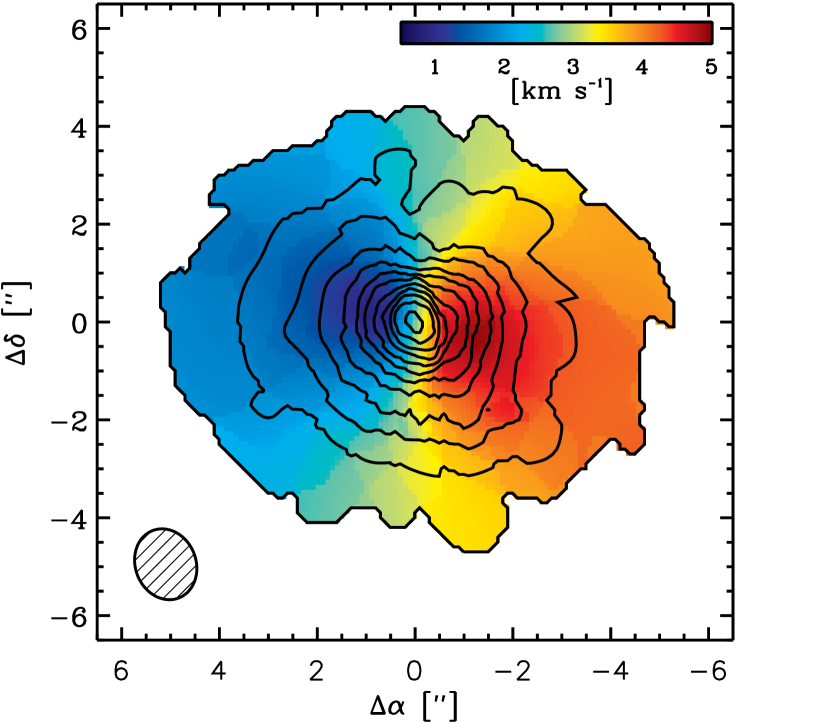
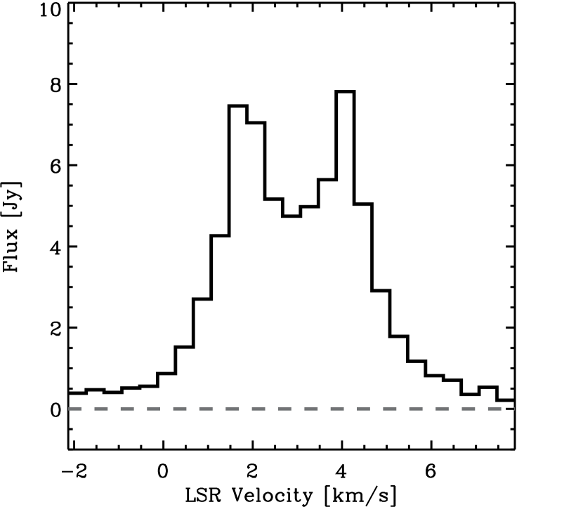
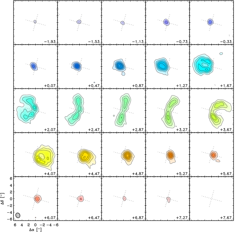
The CO visibilities were continuum-subtracted and truncated outside a projected baseline length of 200 k to reduce the data volume and improve the signal-to-noise ratio. They were then Fourier inverted, deconvolved with the CLEAN algorithm, and restored with a synthesized beam using the MIRIAD package. The naturally-weighted spectral images shown as channel maps in Figure 1 were synthesized on a 0.4 km s-1 smoothed velocity scale with a beam (at a position angle of 24°). The typical RMS noise level in each channel is 70 mJy beam-1. There is CO emission firmly detected (3 ) out to 4.8 km s-1 from the systemic velocity, estimated to be km s-1 (corresponding to km s-1 in the heliocentric frame), with an integrated intensity of Jy km s-1 and a peak flux density of Jy beam-1 ( K; a peak S/N = 21), including the calibration uncertainties. Figure 2 shows a map of the velocity-integrated CO intensities (0th moment; contours) overlaid on the intensity-weighted velocities (1st moment; colorscale), as well as a spatially integrated CO spectrum. These data exhibit a molecular gas disk with a clear rotation pattern, from east (blueshifted) to west (redshifted), and suggest a modest inclination angle to the line of sight. Near the systemic velocity, the CO emission subtends 5″ in radius (365 AU; see Rodriguez et al., 2010).
3 Modeling Analysis
The fundamental goal here is to derive a dynamical estimate of the central stellar mass based on the kinematic properties of the V4046 Sgr gas disk. In order to extract from a measurement of the disk velocity field, we need to construct a detailed physical model of the disk structure.111For the sake of convenient and general notation, we will refer to the central stellar mass as . In this particular case, corresponds to the sum of the stellar masses in the V4046 Sgr binary. We adopt a modeling formalism motivated by Beckwith & Sargent (1993), which makes three basic assumptions about disk properties. First, the disk material is assumed to be orbiting in Keplerian rotation around a point mass, meaning the central stars are treated as one object that dominates the disk velocity field. Previous work has found little evidence to support (simple parametric) deviations from Keplerian -fields in disks (e.g., see Simon et al., 2000); the corollary criterion that the disk mass is only a small fraction of the stellar mass () can be confirmed a posteriori (see §4). Second, the disk is assumed to be geometrically thin at all radii. Although Piétu et al. (2007) argued that this may not be valid at very large radii (800 AU), the higher for the V4046 Sgr binary (which decreases the disk scale height; see below) and the limited extent of the CO emission from its disk (400 AU) suggest it is a reasonable approximation in this case. And third, in the context of the disk structure, we assume that the gas is vertically isothermal and in hydrostatic pressure equilibrium. A more realistic model would include a temperature inversion (e.g., D’Alessio et al., 1998). However, excluding that kind of added complexity does not diminish the accuracy of an estimate: the emission from a single CO line is generated in a narrow vertical layer of the disk atmosphere, which has a roughly constant temperature (Dartois et al., 2003).
The model for the gas density distribution is constructed in cylindrical coordinates (, , ),
| (1) |
where is the radial surface density profile and is the pressure scale height at each radius. We assume a parametric version of the former that is appropriate for an accretion disk with a static, power-law viscosity profile (Lynden-Bell & Pringle, 1974; Hartmann et al., 1998) and is currently the basis for most dust-based disk density measurements (e.g., Andrews et al., 2009, 2010),
| (2) |
where is a density gradient, is a characteristic radius, and is a normalization equivalent to . The scale heights are calculated with the explicit assumption of hydrostatic equilibrium and a constant vertical temperature profile, such that
| (3) |
where is the sound speed, is the angular velocity, is the radial temperature profile, is the Boltzmann constant, is the gravitational constant, is the mass of a hydrogen atom, and is the mean molecular weight of the gas. We further assume a simple power-law behavior for the radial temperature profile,
| (4) |
where is a temperature gradient and is the gas temperature at a radius of 10 AU. The parametric descriptions in Equations (1)-(4) completely characterize the temperature and density structure of a model gas disk. The gas kinematics are described by a Keplerian velocity field,
| (5) |
meaning there is only rotation, and no net motion in the radial or vertical dimensions.
Given a physical disk structure, we can construct a model of the CO =21 emission with the added assumption that the energy levels relevant for this transition are populated according to local thermodynamic equilibrium (LTE). Although the LTE approximation is not always valid in protoplanetary disks, Pavlyuchenkov et al. (2007) demonstrated that it is an appropriate simplification for the low energy and high optical depths associated with this particular species and transition. We model the emission line intensity distribution by integrating the radiative transfer equation along each sight line , so that
| (6) |
where is the absorption coefficient, is the source function (here equivalent to the Planck function), and is the optical depth along the line-of-sight. The absorption coefficient is the sum of contributions from dust and gas. For the former, we assume , where the dust-to-gas mass ratio is and the grain opacity is 100 GHz) cm2 g-1 (Beckwith et al., 1990). In the particular case of the V4046 Sgr disk, the contribution of dust to the absorption coefficient is effectively negligible compared to the gas; the specific choices of and (within reasonable limitations) have no tangible effect on our results (moreover, continuum emission is removed from the data before our modeling analysis).
The absorption coefficient of the CO gas is calculated from the transition cross section weighted by the population of the lower energy level, , such that (note that in this specific case, ). Since we assume the line is thermally populated in LTE, the level populations are determined by the local disk temperature via the Boltzmann equation,
| (7) |
where is the transition energy, is the statistical weight, is the partition function, and is the CO fractional abundance (assumed to be constant everywhere in the disk). The details of the emission line model are encoded in the absorption cross section,
| (8) |
where is the line profile function and the integrated cross section is
| (9) |
where we have used the Einstein relation in the last equality to express the Einstein- coefficient in terms of the Einstein- coefficient provided by the LAMDA molecular database (Schöier et al., 2005). The line profile function naturally determines the shape of the emission line, where a given frequency corresponds to an intrinsic Doppler velocity relative to the line center, . The gas in a given disk model has a projected, line-of-sight velocity field given by , where is the inclination of the disk relative to the observer (such that ° is edge-on; for the geometry, see Isella et al., 2007). The line profile shape at each frequency is determined by the difference between the Doppler and line-of-sight velocities,
| (10) |
and the effective line width, . The latter is comprised of the quadrature sum of contributions from thermal and non-thermal broadening terms,
| (11) |
where is the mean molecular weight of CO and is the contribution from microturbulence. We assume that the turbulent velocity width is constant throughout the disk.
The Beckwith & Sargent (1993) model formalism highlighted above is admittedly complex. A single model is completely described by 14 parameters: four quantify the distribution of CO densities {, , , }, two characterize the temperature structure (and therefore the vertical density structure) {, }, three play pivotal roles describing the disk kinematics {, , }, and the remaining five relate the model to the observations – i.e., convert from physical coordinates in the disk to the observed plane projected on the sky – including the disk inclination and major axis position angle {, PAd}, distance {}, and disk center {, }. Some of these parameters can be reliably determined in a simple way, and then fixed to facilitate the data modeling problem (with no tangible impact on the quality of the determination). In this case, the systemic LSR velocity (effectively ) was measured directly from the SMA data and set to km s-1. The disk center coordinates were estimated from both the dust continuum and CO emission morphology at the systemic velocity (see Fig. 1) and set to , (J2000), coincident with the composite V4046 Sgr stellar position in the UCAC3 catalog (Zacharias et al., 2010). We adopted the distance inferred by Torres et al. (2006) from the kinematic parallax (moving cluster) technique, pc (but see §5 regarding alternative values).
Some additional practical simplications can be made, since the focus here is on the velocity field and not the disk structure details. Because the line opacity is so much greater than the dust opacity, the normalization parameters and are not independent: we can only constrain their product. In practice, we adopt a joint CO disk mass parameter, , for that purpose. Moreover, after extensive experimentation, we concluded that two more parameters should be fixed. First, we found that the disk orientation was very well-determined (within 1°) at PA (E of N), so that continued iteration on a more precise value was a waste of computational resources: fixing this parameter has negligible quantitative impact on the other model parameters or their uncertainties. And second, we fixed the surface density gradient, . The key parameters that set the density profile, {, } are anti-correlated and strongly degenerate; statistically indistinguishable model fits can be found over a large range of these parameters. The degeneracy is remarkably narrow, and could easily be missed with standard minimization algorithms (resulting in local minima with misleadingly tight constraints on the gradient). Fortunately, this degeneracy has minimal impact on the parameters most relevant for characterizing the disk velocity field: the precision and accuracy of a determination are not notably affected by the uncertainties in {, }. With that in mind, we have made the modeling process more tractable with a fixed .
Making use of those simplifications, a synthetic CO spectral datacube can be calculated by specifying 7 free parameters, {, , , , , , }. That model datacube is then resampled at the observed velocities and spatial frequencies and processed in the same way as the data (see §2) to produce a set of synthetic spectral visibilities. Those model visibilities are evaluated with respect to the data by computing a composite value, summed over the real and imaginary components in 25 spectral channels. The best-fit set of model parameters and their associated uncertainties were determined with a Monte Carlo Markov Chain (MCMC) technique, using the affine invariant ensemble sampler developed by Goodman & Weare (2010, see also Foreman-Mackey et al. 2012), using a jump probability . To our knowledge, this is the first application of these more sophisticated MCMC methods for parameter estimation in this particular context: previous studies have relied on downhill simplex routines (e.g., Guilloteau & Dutrey, 1998; Simon et al., 2000), sometimes with clever modifications to address asymmetric uncertainties (Piétu et al., 2007). Although comparatively the MCMC technique is computationally expensive, this Bayesian treatment has the distinct advantage of providing the posterior probability distributions for each parameter in the complex, multi-dimensional parameter-space of the underlying disk model.
4 Results
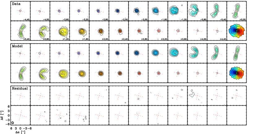
The best-fit model derived from the SMA data is compiled in Table 1, which lists the mode (peak) of the posterior probability distribution for each parameter along with its uncertainty, based on the range of values that encompass 68% of the distribution area (i.e., 1 uncertainties for a Gaussian distribution). Figure 3 makes a direct comparison between the data and the best-fit model in the spectral image plane, demonstrating the fit quality with only low-level (statistically insignificant) residuals present in the channel maps. The best-fit model has a reduced . A more detailed view of the multi-dimensional results of the modeling analysis is presented in Figure 4, where we have taken the 30,000 MCMC samples computed and marginalized over parameter subsets to display one and two-parameter posterior probability distributions. The marginalized distributions for individual parameters are single-peaked, while the paired distributions highlight internal degeneracies in the model. For example, there are tight correlations between normalizations and sizes (e.g., {, }, to conserve the integrated line intensity; this would be modified were a free parameter) or gradients (e.g., {, }, to maintain an appropriate temperature in the outer disk; Mundy et al., 1996; Andrews & Williams, 2007), as well as more subtle associations amongst parameters related to line broadening (amongst , , and ; Guilloteau & Dutrey, 1998; Hughes et al., 2011). The degeneracy of most interest here is the {, } anti-correlation, which is a natural consequence of reproducing the observed line-of-sight velocity pattern, (i.e., ).
The best-fit model parameters that describe the V4046 Sgr disk structure are typical for young protoplanetary disks. The adopted (fixed) surface density gradient () and characteristic radius ( AU) lie near the median values for a survey of disk structures in the Ophiuchus region (Andrews et al., 2009, 2010); the temperature profile ( K, ; and therefore vertical density distribution) and turbulent linewidth ( km s-1) are comparable to those inferred from CO emission in other T Tauri disks (e.g., Guilloteau & Dutrey, 1998; Piétu et al., 2007; Hughes et al., 2008, 2011). If we assume the CO mass fraction found in dark clouds () is also applicable in the disk, the molecular density normalization parameter implies a modest gas mass, M⊙, validating a posteriori our assumption that self-gravity is negligible (). In any case, our simple treatment of the disk structure is really only used as a means to an end: the focus here is to place a firm constraint on the key parameter that determines the behavior of the disk velocity field – the central stellar mass, .

We infer a total stellar mass of M⊙ for the V4046 Sgr spectroscopic binary, a formally precise constraint with a relative uncertainty of 3-5%. Figure 4 demonstrates that this estimate of is essentially independent of the disk structure parameters in the model. The sole relevant degeneracy is with the disk inclination, which we infer to be (a relative precision of 2-5%). Within the quoted uncertainties, these {, } values are consistent with the previous determinations by Rodriguez et al. (2010), who used a simple grid search and an altogether different underlying disk structure model. These {, } measurements based on the circumstellar gas disk kinematics can be directly compared with the joint (degenerate) constraints on {, } imposed by RV measurements of the spectroscopic binary itself. Although various groups have studied this SB2 system (Quast et al., 2000; Stempels & Gahm, 2004; Donati et al., 2011), by far the most robust constraints on the stellar parameters come from the long-term, extensive, and high resolution optical spectroscopic monitoring campaign conducted by Stempels (2012). In that work, the RV data are found to be best explained with a binary that has a total mass M⊙. The inset in Figure 4 confirms that our disk kinematics constraints and the RV constraints by Stempels (2012) coincide in the stellar massinclination plane: the two completely independent methods find the same results well within their formal 1 uncertainties. Adopting our best estimate of and propagating the relevant uncertainties, the RV constraints suggest that . Therefore, we quantitatively confirm the finding of Rodriguez et al.: the V4046 Sgr spectroscopic binary and its associated, large-scale circumbinary disk are co-planar within across 4 orders of magnitude in radial scale.
5 Discussion
We have presented spatially and spectrally resolved Submillimeter Array observations of the 12CO =21 line emission from the isolated, nearby, and gas-rich circumstellar disk that orbits the close, pre-main sequence double-lined spectroscopic binary V4046 Sgr. Adopting a simple parametric model for the structure of a flared Keplerian disk, we employ a Monte Carlo Markov Chain technique to infer the properties of the disk velocity field from these data, and thereby provide a robust statistical estimate for the total mass of the central binary. We find that these CO line data are best reproduced for a binary mass M⊙ and a disk viewing angle inclined by from face-on. Those values are in excellent agreement with the completely independent inferences of Stempels (2012), made from their extensive radial velocity monitoring campaign of the spectroscopic binary itself. The orbital planes of the binary ( AU) and its associated circumbinary disk (on radial scales out to 400 AU) are aligned within 0.11°. These results demonstrate that, despite its complexity, the disk-based kinematic method for estimating the masses of young stars is both precise (at the level of a few percent) and accurate in an absolute sense, as verified here by an entirely independent dynamical constraint.
The disk-based dynamical estimate of can be combined with the RV constraints of Stempels (2012) and other information from the literature to assess the predictions of pre-MS stellar evolution models. Coupling our estimate with the stellar mass ratio () and mass function () determined by Stempels, we can derive the masses of the individual stellar components in the V4046 Sgr binary, and M⊙, and their orbital inclination, .222Here and throughout, we conservatively adopt the larger of all asymmetric uncertainties for simplicity. Assuming that the stellar rotation axes are aligned with the binary orbital axis (a spin-orbit alignment presumably induced by tides in this close, circularized system; e.g., Zahn, 1977; Hut, 1981; Melo et al., 2001), the radial and rotational velocities measured for each stellar component by Stempels can be used to determine the stellar radii, and R⊙. Stempels & Gahm (2004) inferred spectral types of K5 and K7 in this system, corresponding to effective temperatures of and K for the standard conversion advocated by Schmidt-Kaler (1982); an ambiguity of one spectral subclass has been assumed to estimate the temperature uncertainties. Those measurements imply that the individual stellar luminosities are and L⊙ (a total luminosity of L⊙).
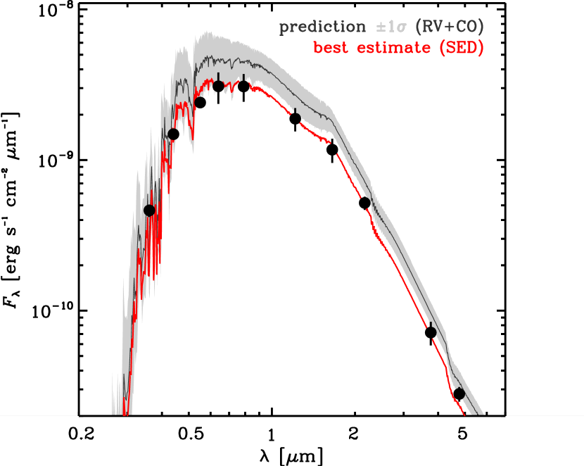
Figure 5 shows the composite optical/near-infrared spectrum expected from the V4046 Sgr binary, given the effective temperatures, stellar radii, and masses derived above from the combination of RV data and our disk-based measurements (black curve, with uncertainty in shaded gray). This spectral energy distribution (SED) prediction was generated from an interpolated grid of Lejeune et al. (1997) model spectra, assuming the appropriate stellar gravities ( in both cases), negligible interstellar reddening (), and our adopted pc. Representative broadband photometric data are marked as the datapoints in Figure 5, constructed from the weighted mean magnitudes of Hutchinson et al. (1990), Strassmeier et al. (1993), Jensen & Mathieu (1997), and the 2MASS (Skrutskie et al., 2006) and DENIS (Epchtein et al., 1997) surveys: uncertainties were taken as the quadrature sum of the standard deviation of the weighted mean and the maximal deviation from the weighted mean, in an effort to more faithfully represent potential uncertainties due to variability. A quick examination of Figure 5 demonstrates that the spectral morphology of the data and model prediction are a good match, although the normalizations appear discrepant. Scaling the (best-fit) predicted spectrum down by 30% provides a good match to the observed spectrum; a composite luminosity of L⊙ is more appropriate (red curve). Therefore, the predicted and observed composite binary luminosities are marginally (1.4 ) different.
Although formally the conflict in these luminosity values is not statistically significant, it is still interesting to consider some potential paths for a better reconciliation of all the data. Perhaps the most straightforward means of doing so is to modify the assumed distance to the system: taken at face value, a 30% increase to pc implies an inherently more luminous pair of stars with a spectrum that would be in good agreement with the observations. However, that same re-normalization impacts the total stellar mass inferred from the CO data, with a linear scaling to M⊙ that introduces a substantial (2 ) discrepancy in the {, }-plane between the disk-kinematics and RV techniques for estimating stellar parameters. Although it hardly seems worthwhile to trade one marginal discrepancy for another (which is technically less marginal), there is no a priori reason that the orbital planes of the disk and binary need to be aligned with the precision inferred in §4. Unfortunately, little guidance is provided in the form of an uncertainty on the kinematic parallax measurement of Torres et al. (2006). In any case, discrepancies in effective temperatures and luminosities are not necessarily uncommon for active young stars (Stassun et al., 2012), and particularly for those in close binary systems (e.g., Goméz Maqueo Chew et al., 2012).
Ultimately, dwelling on a marginal luminosity discrepancy is not well justified, especially given the independent distance estimate from the Torres et al. (2006) study. In the following, we adopt the stellar parameters inferred from the joint constraints of the CO disk spatio-kinematics and the optical RV studies of Stempels assuming pc, but use individual stellar luminosities scaled down by 30% to best match the observed optical and near-infrared spectrum: L⊙ and L⊙ (note that each component is slightly less luminous than reported by Donati et al., 2011). With those results, we can make comparisons with the predictions of pre-MS evolution models to estimate the ages () and masses of the individual stars in the V4046 Sgr binary. To accomplish that, we follow the Bayesian methodology of Jørgensen & Lindegren (2005), which employs a finely-interpolated grid of pre-MS models in the HR diagram to estimate the probability distributions of stellar mass and age given the measured values (and uncertainties) of effective temperatures and luminosities (see also Gennaro et al., 2012). If we define the observables as {, } = {, } with associated uncertainties {, }, and the pre-MS model predictions {, , , }, we can write the likelihood function as a multivariate Gaussian,
| (12) |
The best-fit {, } are then directly determined from the {, } that maximize the likelihood, with uncertainties that can be calculated from the shape of the likelihood distribution. This procedure was conducted for four different pre-MS evolution models, assuming solar composition, a fractional deuterium abundance of , and a convective mixing parameter -2.0: D’Antona & Mazzitelli (1998), Baraffe et al. (1998), Siess et al. (2000), and Tognelli et al. (2011).
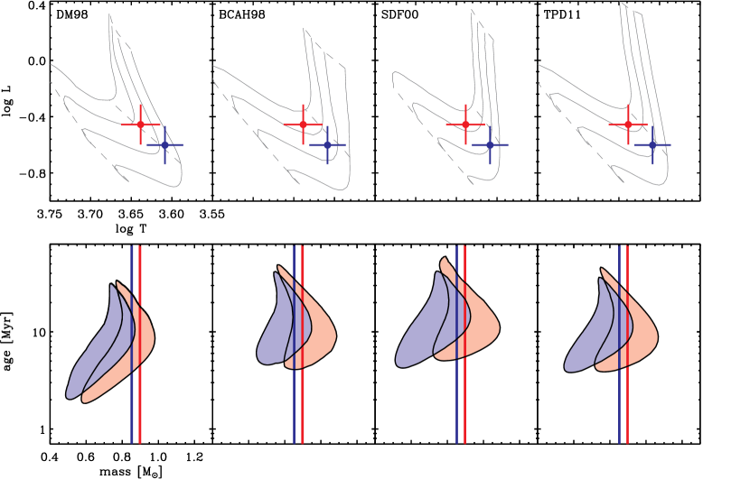
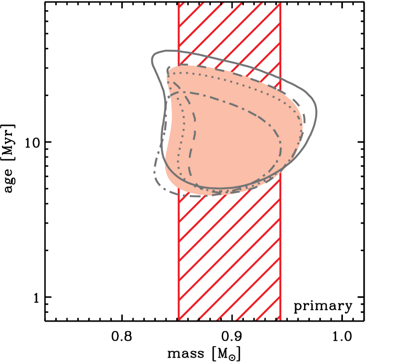
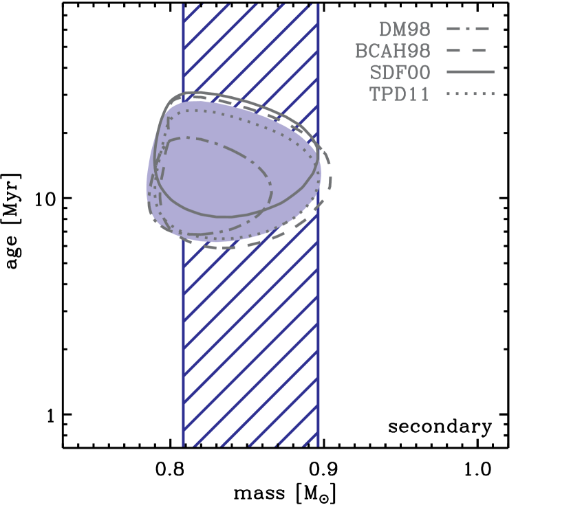
The results of these comparisons are presented in Table 2. Figure 6 shows the V4046 Sgr stellar properties that were inferred from each of the four reference sets of pre-MS evolutionary model tracks in the HR diagram. All of the evolutionary models make predictions for the V4046 Sgr stellar masses that are remarkably consistent with each other and the dynamical masses inferred in §4. The stellar masses that formally maximize the likelihood in Equation 12 are systematically 2-10% below the best-fit dynamical masses, an under-prediction typical of pre-MS models regardless of the dynamical method used to estimate (Hillenbrand & White, 2004; Gennaro et al., 2012). However, those modest discrepancies are not statistically significant, given the uncertainties on {, } and the dynamical masses. An examination of Figure 6 demonstrates that the V4046 Sgr stars are nearly evolved off the Hayashi track, having presumably developed radiative cores as expected for their solar-like masses. The clear implication of their location in the HR diagram is that the V4046 Sgr binary is comparatively old for a pre-MS system, as has been previously reported by Donati et al. (2011) and Kastner et al. (2011). The models used here suggest a large range of ages are plausible, from 5-30 Myr, and confirm that the binary components are coeval. If we include a Gaussian prior representing the dynamical masses into the Bayesian analysis of the HR diagrams described above (labeled as ‘+dyn’ in Table 2), we can infer a smaller range of acceptable “dynamical” ages from each set of pre-MS models. The different pre-MS model predictions with these dynamical priors are shown together, and averaged (weighted by the posterior probability for each model; Hoeting et al., 1999), in Figure 7: the averaged results suggest ages of and Myr for V4046 Sgr A and B, respectively. The corresponding coeval age is 13 Myr, in good agreement with the age constraints from the putative far-flung companion(s) V4046 Sgr C[D] (at a separation of 12,350 AU, or 28 on the sky; Kastner et al., 2011).
Torres et al. (2006) suggested that the observed space motion of V4046 Sgr is consistent with a high probability of membership in the Pic moving group, a widespread and local ( pc) stellar association with an age range estimated to be 8-20 Myr (e.g., Zuckerman et al., 2001; Zuckerman & Song, 2004; Torres et al., 2008). The kinematic parallax calculated by Torres et al. ( pc) and component ages estimated here for the V4046 Sgr binary are certainly supportive of that conclusion. If that is the case, it is worth noting the uniqueness of the V4046 Sgr circumstellar environment: there are no other Pic moving group members that are known to host such a massive, long-lived, gas-rich accretion disk. Regardless of its original association, the proximity and advanced age of V4046 Sgr make for a remarkable case study in both the long-term evolution of protoplanetary disk structure and the fundamental properties of pre-MS binary stars.
Although V4046 Sgr is a particularly striking example of the methodology behind disk-based dynamical estimates of stellar masses, we anticipate that these techniques will find considerably more use in the near future as the Atacama Large Millimeter Array (ALMA) project is completed. Even with vastly improved data quality, this simplified model to extract the gas disk rotation curve from such interferometric observations (see §3) remains complex. However, we have demonstrated that the method is robust, accurate, and precise, by using independent dynamical constraints from the V4046 Sgr spectroscopic binary radial velocity monitoring results. In practice, these constraints and others like them (notably for UZ Tau E; see Simon et al., 2000; Prato et al., 2002) effectively serve as a check on the absolute calibration of the modeling technique described in §3. The consistency between the independent dynamical constraints on the V4046 Sgr stellar masses validates the application of this procedure to dynamically “weigh” single, isolated pre-MS stars based on their gas disk kinematics. Along with an investment in accurate stellar luminosity and temperature measurements, ALMA observations of the molecular gas kinematics in circumstellar disks will usher in a new era of precision in the fundamental astrophysical properties of young stars.
6 Summary
We have presented sensitive, high-resolution SMA observations of the 12CO =21 line emission from the massive, gas-rich disk orbiting the double-lined spectroscopic binary star V4046 Sgr. Using simple radiation transfer calculations for a disk structure model with a Keplerian velocity field, we fit the observed spectral visibilities using a stochastic model optimization technique that simultaneously infers model parameter values and their uncertanties. Our specific focus has been on the key model parameters that describe the disk velocity field, with a goal of placing a firm, dynamical constraint on the mass of the central binary. The key conclusions of our analysis are:
-
1.
From modeling the CO line emitted by the circumbinary disk, we infer that the total stellar mass of the V4046 Sgr binary is , assuming the kinematic parallax distance of 73 pc estimated by Torres et al. (2006). That measurement is in excellent agreement with the independent dynamical constraints imposed from the analysis of an optical spectroscopic monitoring campaign of the radial velocity variations from the binary itself (Stempels, 2012).
-
2.
The mutual consistency of these distinct dynamical constraints on the stellar masses verifies that the mass determination based on the velocity field of the disk gas is accurate in an absolute sense, as well as remarkably precise (with a 3-5% formal uncertainty on ).
-
3.
That same combination of constraints from millimeter and optical spectroscopic measurements confirm that the orbital planes of the stars and their accompanying circumbinary disk are co-planar, with inferred inclination angles ( and ) that differ by ° over roughly four decades in radius, from 0.04 to 400 AU.
-
4.
The inferred component masses of the V4046 Sgr binary are in uniformly good agreement with a variety of pre-MS evolution model predictions. When combined with our dynamical constraints, those same models confirm the coevality of the binary components, and suggest an average age for the system of Myr. Therefore, V4046 Sgr hosts one of the oldest and nearest gas-rich primordial accretion disks currently known.
| parameter | units | estimate |
|---|---|---|
| [AU] | ||
| [K] | ||
| [km s-1] | ||
| [∘] | ||
| [M⊙] |
Note. — See §3 for a description of the model parameters. The uncertainties for each parameter are determined from the width of the posterior distribution that encapsulates 68% of the models around the peak (equivalent to for Gaussian random variables.
| V4046 Sgr A | V4046 Sgr B | ||||||||
|---|---|---|---|---|---|---|---|---|---|
| [M⊙] | [Myr] | ||||||||
| Models | HR | +dyn | HR | +dyn | HR | +dyn | HR | +dyn | |
| DM98 | |||||||||
| BCAH98 | |||||||||
| SDF00 | |||||||||
| TPD11 | |||||||||
| mean | |||||||||
Note. — Stellar mass and age estimates from the four different pre-MS evolution models are calculated using the HR observables {, }, following the methods outlined in §5. We report results for both a uniform (HR) and Gaussian (+dyn) prior on the mass, with the latter based on the dynamical constraints. The mean values are computed for all the models, following the technique outlined by Hoeting et al. (1999).
References
- Alibert et al. (2011) Alibert, Y., Mordasini, C., & Benz, W. 2011, A&A, 526, 63
- Andrews & Williams (2007) Andrews, S. M., & Williams, J. P. 2007, ApJ, 659, 705
- Andrews et al. (2009) Andrews, S. M., Wilner, D. J., Hughes, A. M., Qi, C., & Dullemond, C. P. 2009, ApJ, 700, 1502
- Andrews et al. (2010) Andrews, S. M., Wilner, D. J., Hughes, A. M., Qi, C., & Dullemond, C. P. 2010, ApJ, 723, 1241
- Artymowicz & Lubow (1994) Artymowicz, P., & Lubow, S. H. 1994, ApJ, 421, 651
- Baraffe et al. (1998) Baraffe, I., Chabrier, G., Allard, F., & Hauschildt, P. H. 1998, A&A, 337, 403
- Baraffe et al. (2002) Baraffe, I., Chabrier, G., Allard, F., & Hauschildt, P. H. 2002, A&A, 382, 563
- Baraffe et al. (2009) Baraffe, I., Chabrier, G., & Gallardo, J. 2009, ApJ, 702, L27
- Baraffe & Chabrier (2010) Baraffe, I., & Chabrier, G. 2010, A&A, 521, 44
- Bastian et al. (2010) Bastian, N., Covey, K. R., & Meyer, M. R. 2010, ARA&A, 48, 339
- Beckwith et al. (1990) Beckwith, S. V. W., Sargent, A. I., Chini, R. S., & Güsten, R. 1990, AJ, 99, 924
- Beckwith & Sargent (1993) Beckwith, S. V. W., & Sargent, A. I. 1993, ApJ, 402, 280
- Boden et al. (2005) Boden, A. F., Sargent, A. I., Akeson, R. L., et al. 2005, ApJ, 635, 442
- Boden et al. (2007) Boden, A. F., Torres, G., Sargent, A. I., et al. 2007, ApJ, 670, 1214
- Boden et al. (2009) Boden, A. F., Akeson, R. L., Sargent, A. I., et al. 2009, ApJ, 696, L111
- Boden et al. (2012) Boden, A. F., Torres, G., Duchêne, G., et al. 2012, ApJ, 747, 17
- Byrne (1986) Byrne, P. B. 1986, Ir. Astron. J., 17, 294
- D’Alessio et al. (1998) D’Alessio, P., Canto, J., Calvet, N., & Lizano, S. 1998, ApJ, 500, 411
- D’Antona & Mazzitelli (1998) D’Antona, F., & Mazzitelli, I. 1998, in ASP Conf. Ser. 134, Brown Dwarfs and Extrasolar Planets, ed. R. Rebolo, E. L. Martin, & M. R. Z. Osorio (San Francisco, CA: ASP), 442
- D’Antona et al. (2000) D’Antona, F., Ventura, P., & Mazzitelli, I. 2000, ApJ, 543, L77
- Dartois et al. (2003) Dartois, E., Dutrey, A., & Guilloteau, S. 2003, A&A, 399, 773
- Donati et al. (2011) Donati, J.-F., et al. 2011, MNRAS, 417, 1747
- Duchêne et al. (2006) Duchêne, G., Beust, H., Adjali, F., Konopacky, Q. M., & Ghez, A. M. 2006, A&A, 457, L9
- Dutrey et al. (1994) Dutrey, A., Guilloteau, S., & Simon, M. 1994, A&A, 286, 149
- Dutrey et al. (1998) Dutrey, A., Guilloteau, S., Prato, L., Simon, M., Duvert, G., Schuster, K., & Ménard, F. 1998, A&A, 338, L63
- Epchtein et al. (1997) Epchtein, N., et al. 1997, Messenger, 87, 27
- Foreman-Mackey et al. (2012) Foreman-Mackey, D., Hogg, D. W., Lang, D., & Goodman, J. 2012, arXiv:1202.3665
- Gennaro et al. (2012) Gennaro, M., Prada Moroni, P. G., & Tognelli, E. 2012, MNRAS, 420, 986
- Goodman & Weare (2010) Goodman, J., & Weare, J. 2010, Comm. App. Math. Comp. Sci., 5, 65
- Goméz Maqueo Chew et al. (2012) Goméz Maqueo Chew, Y., et al. 2012, ApJ, 745, 58
- Guilloteau & Dutrey (1998) Guilloteau, S., & Dutrey, A. 1998, A&A, 339, 467
- Hartmann et al. (1998) Hartmann, L., Calvet, N., Gullbring, E., & D’Alessio, P. 1998, ApJ, 495, 385
- Hillenbrand & White (2004) Hillenbrand, L. A., & White, R. J. 2004, ApJ, 604, 741
- Ho et al. (2004) Ho, P. T. P., Moran, J. M., & Lo, K. Y. 2004, ApJ, 616, L1
- Hoeting et al. (1999) Hoeting, J. A., Madigan, D., Raftery, A. E., & Volinsky, C. T. 1999, Statist. Sci., 14, 4
- Hughes et al. (2008) Hughes, A. M., Wilner, D. J., Qi, C., & Hogerheijde, M. R. 2008, ApJ, 678, 1119
- Hughes et al. (2011) Hughes, A. M., Wilner, D. J., Andrews, S. M., Qi, C., & Hogerheijde, M. R. 2011, ApJ, 727, 85
- Hut (1981) Hut, P. 1981, A&A, 99, 126
- Hutchinson et al. (1990) Hutchinson, M. G., Evans, A., Winkler, H., & Spencer Jones, J. 1990, A&A, 234, 230
- Isella et al. (2007) Isella, A., Testi, L., Natta, A., Neri, R., Wilner, D., & Qi, C. 2007, A&A, 469, 213
- Jensen & Mathieu (1997) Jensen, E. L. N., & Mathieu, R. D. 1997, AJ, 114, 301
- Jørgensen & Lindegren (2005) Jørgensen, B. R., & Lindegren, L. 2005, A&A, 436, 127
- Kastner et al. (2008) Kastner, J. H., Zuckerman, B., Hily-Blant, P., & Forveille, T. 2008, A&A, 492, 469
- Kastner et al. (2011) Kastner, J. H., Sacco, G. G., Montez, R., et al. 2011, ApJ, 740, L17
- Koerner et al. (1993) Koerner, D. W., Sargent, A. I., & Beckwith, S. V. W. 1993, Icarus, 106, 2
- Lejeune et al. (1997) Lejeune, T., Cuisinier, F., & Buser, R. 1997, A&AS, 125, 229
- Lynden-Bell & Pringle (1974) Lynden-Bell, D., & Pringle, J. E. 1974, MNRAS, 168, 603
- Mathieu et al. (1989) Mathieu, R. D., Walter, F. A., & Myers, P. C. 1989, AJ, 98, 987
- Mathieu et al. (1991) Mathieu, R. D., Adams, F. C., & Latham, D. W. 1991, AJ, 101, 2184
- Mathieu et al. (1997) Mathieu, R. D., et al. 1997, AJ, 113, 1841
- Melo et al. (2001) Melo, C. H. F., Covino, E., Alcalá, J. M., & Torres, G. 2001, A&A, 378, 898
- Mendes et al. (1999) Mendes, L. T. S., D’Antona, F., & Mazzitelli, I. 1999, A&A, 341, 174
- Morales-Calderón et al. (2012) Morales-Calderón, M., Stauffer, J. R., Stassun, K. G., et al. 2012, ApJ, 753, 149
- Mundy et al. (1996) Mundy, L. G., et al. 1996, ApJ, 464, L169
- Öberg et al. (2011) Öberg, K. I., et al. 2011, ApJ, 734, 98
- Pavlyuchenkov et al. (2007) Pavlyuchenkov, Y., Semenov, D., Henning, T., Guilloteau, S., Piétu, V., Launhardt, R., & Dutrey, A. 2007, ApJ, 669, 1262
- Piétu et al. (2007) Piétu, V., Dutrey, A., & Guilloteau, S. 2007, A&A, 467, 163
- Prato et al. (2002) Prato, L., Simon, M., Mazeh, T., Zucker, S., & McLean, I. S. 2002, ApJ, 579, L99
- Quast et al. (2000) Quast, G. R., Torres, C. A. O., de La Reza, R., da Silva, L., & Mayor, M. 2000, IAU Symposium, 200, 28P
- Rodriguez et al. (2010) Rodriguez, D. R., Kastner, J. H., Wilner, D., & Qi, C. 2010, ApJ, 720, 1684
- Schaefer et al. (2003) Schaefer, G. H., Simon, M., Nelan, E., & Holfeltz, S. T. 2003, AJ, 126, 1971
- Schaefer et al. (2006) Schaefer, G. H., Simon, M., Beck, T. L., Nelan, E., & Prato, L. 2006, AJ, 132, 2618
- Schaefer et al. (2008) Schaefer, G. H., Simon, M., Prato, L., & Barman, T. 2008, AJ, 135, 1659
- Schmidt-Kaler (1982) Schmidt-Kaler, T. 1982, in Landölt Bornstein, Group VI, Vol. 2, ed. K.-H. Hellwege (Berlin: Springer), 454
- Schöier et al. (2005) Schöier, F. L., van der Tak, F. F. S., van Dishoeck, E. F., & Black, J. H. 2005, A&A, 432, 369
- Simon et al. (2000) Simon, M., Dutrey, A., & Guilloteau, S. 2000, ApJ, 545, 1034
- Siess et al. (1997) Siess, L., Forestini, M., & Dougados, C. 1997, A&A, 326, 1001
- Siess & Livio (1997) Siess, L., & Livio, M. 1997, ApJ, 490, 785
- Siess et al. (2000) Siess, L., Dufour, E., & Forestini, M. 2000, A&A, 358, 593
- Skrutskie et al. (2006) Skrutskie, M. F., et al. 2006, AJ, 131, 1163
- Stassun et al. (2004) Stassun, K. G., Mathieu, R. D., Vaz, L. P. R., Stroud, N., & Vrba, F. J. 2004, ApJS, 151, 357
- Stassun et al. (2012) Stassun, K. G., Kratter, K. M., Scholz, A., & Dupuy, T. J. 2012, ApJ, in press (arXiv:1206.4930)
- Steffen et al. (2001) Steffen, A. T., et al. 2001, AJ, 122, 997
- Stempels & Gahm (2004) Stempels, H. C., & Gahm, G. F. 2004, A&A, 421, 1159
- Stempels (2012) Stempels, H. C., 2012, in preparation
- Strassmeier et al. (1993) Strassmeier, K. G., Hall, D. S., Fekel, F. C., & Scheck, M. 1993, A&AS, 100, 173
- Tamazian et al. (2002) Tamazian, V. S., Docobo, J. A., White, R. J., & Woitas, J. 2002, ApJ, 578, 925
- Tognelli et al. (2011) Tognelli, E., Prada Moroni, P. G., & Degl’Innocenti, S. 2011, A&A, 533, A109
- Torres et al. (2006) Torres, C. A. O., Quast, G. R., da Silva, L., de la Reza, R., Melo, C. H. F., & Sterzik, M. 2006, A&A, 460, 695
- Torres et al. (2008) Torres, C. A. O., Quast, G. R., Melo, C. H. F., & Sterzik, M. F. 2008, Handbook of Star Forming Regions, Volume II, 757
- Zacharias et al. (2010) Zacharias, N., et al. 2010, AJ, 139, 2184
- Zahn (1977) Zahn, J.-P. 1977, A&A, 57, 383
- Zuckerman et al. (2001) Zuckerman, B., Song, I., Bessell, M. S., & Webb, R. A. 2001, ApJ, 562, L87
- Zuckerman & Song (2004) Zuckerman, B., & Song, I. 2004, ARA&A, 42, 685