Four Soviets Walk the Dog—Improved Bounds for Computing the Fréchet Distance

Abstract

Given two polygonal curves in the plane, there are many ways to define a notion of similarity between them. One popular measure is the Fréchet distance. Since it was proposed by Alt and Godau in 1992, many variants and extensions have been studied. Nonetheless, even more than 20 years later, the original $O(n^{2}\log n)$ algorithm by Alt and Godau for computing the Fréchet distance remains the state of the art (here, $n$ denotes the number of edges on each curve). This has led Helmut Alt to conjecture that the associated decision problem is 3SUM-hard.

In recent work, Agarwal et al. show how to break the quadratic barrier for the discrete version of the Fréchet distance, where one considers sequences of points instead of polygonal curves. Building on their work, we give a randomized algorithm to compute the Fréchet distance between two polygonal curves in time $O(n^{2}\sqrt{\log n}(\log\log n)^{3/2})$ on a pointer machine and in time $O(n^{2}(\log\log n)^{2})$ on a word RAM. Furthermore, we show that there exists an algebraic decision tree for the decision problem of depth $O(n^{2-\varepsilon})$, for some $\varepsilon>0$. We believe that this reveals an intriguing new aspect of this well-studied problem. Finally, we show how to obtain the first subquadratic algorithm for computing the weak Fréchet distance on a word RAM.

1 Introduction

Shape matching is a fundamental problem in computational geometry, computer vision, and image processing. A simple version can be stated as follows: given a database $\mathcal{D}$ of shapes (or images) and a query shape $S$, find the shape in $\mathcal{D}$ that most resembles $S$. However, before we can solve this problem, we first need to address an issue: what does it mean for two shapes to be “similar”? In the mathematical literature, on can find many different notions of distance between two sets, a prominent example being the Hausdorff distance. Informally, the Hausdorff distance is defined as the maximal distance between two elements when every element of one set is mapped to the closest element in the other. It has the advantage of being simple to describe and easy to compute for discrete sets. In the context of shape matching, however, the Hausdorff distance often turns out to be unsatisfactory: it does not take the continuity of the shapes into account. There are well known examples where the distance fails to capture the similarity of shapes as perceived by human observers [6].

In order to address this issue, Alt and Godau introduced the Fréchet distance into the computational geometry literature [45, 8]. They argued that the Fréchet distance is better suited as a similarity measure, and they described an $O(n^{2}\log n)$ time algorithm to compute it on a real RAM or pointer machine. Since Alt and Godau’s seminal paper, there has been a wealth of research in various directions, such as extensions to higher dimensions [7, 29, 24, 27, 34, 46], approximation algorithms [9, 10, 37], the geodesic and the homotopic Fréchet distance [30, 35, 38, 48], and much more [2, 15, 23, 26, 36, 51, 54, 55]. Most known approximation algorithms make further assumptions on the curves, and only an $O(n^{2})$-time approximation algorithm is known for arbitrary polygonal curves [25]. The Fréchet distance and its variants, such as dynamic time-warping [13], have found various applications, with recent work particularly focusing on geographic applications such as map-matching tracking data [16, 63] and moving objects analysis [20, 21, 47].

Despite the large amount of published research, the original algorithm by Alt and Godau has not been improved, and the quadratic barrier on the running time of the associated decision problem remains unbroken. If we cannot improve on a quadratic bound for a geometric problem despite many efforts, a possible culprit may be the underlying 3SUM-hardness [44]. This situation induced Helmut Alt to make the following conjecture.

Conjecture 1.1 (Alt’s Conjecture).

Let $P$, $Q$ be two polygonal curves in the plane. Then it is 3SUM-hard to decide whether the Fréchet distance between $P$ and $Q$ is at most $1$.

Here, $1$ can be considered as an arbitrary constant, which can be changed to any other bound by scaling the curves. So far, the best unconditional lower bound for the problem is $\Omega(n\log n)$ steps in the algebraic computation tree model [22].

Recently, Agarwal et al. [1] showed how to achieve a subquadratic running time for the discrete version of the Fréchet distance, running in $O\left(n^{2}\,\frac{\log\log n}{\log n}\right)$ time. Their approach relies on reusing small parts of the solution. We follow a similar approach based on the so-called Four-Russian-trick which precomputes small recurring parts of the solution and uses table-lookup to speed up the whole computation. The result by Agarwal et al. is stated in the word RAM model of computation. They ask whether their result can be generalized to the case of the original (continuous) Fréchet distance.

Our contribution

We address the question by Agarwal et al. and show how to extend their approach to the Fréchet distance between two polygonal curves. Our algorithm requires total expected time $O(n^{2}\sqrt{\log n}(\log\log n)^{3/2})$. This is the first algorithm with a running time of $o(n^{2}\log n)$ and constitutes the first improvement for the general case since the original paper by Alt and Godau [8]. To achieve this running time, we give the first subquadratic algorithm for the decision problem of the Fréchet distance. We emphasize that these algorithms run on a real RAM/pointer machine and do not require any bit-manipulation tricks. Therefore, our results are more in the line of Chan’s recent subcubic-time algorithms for all-pairs-shortest paths [31, 32] or recent subquadratic-time algorithms for min-plus convolution [17] than the subquadratic-time algorithms for 3SUM due to Baran et al. [12]. If we relax the model to allow constant time table-lookups, the running time can be improved to be almost quadratic, up to $O(\log\log n)$ factors. As in Agarwal et al., our results are achieved by first giving a faster algorithm for the decision version, and then performing an appropriate search over the critical values to solve the optimization problem.

In addition, we show that non-uniformly, the Fréchet distance can be computed in subquadratic time. More precisely, we prove that the decision version of the problem can be solved by an algebraic decision tree [11] of depth $O(n^{2-\varepsilon})$, for some fixed $\varepsilon>0$. It is, however, not clear how to implement this decision tree in subquadratic time, which hints at a discrepancy between the decision tree and the uniform complexity of the Fréchet problem.

Finally, we consider the weak Fréchet distance, where we are allowed to walk backwards along the curves. In this case, our framework allows us to achieve a subquadratic algorithm on the work RAM. Refer to Table 1 for a comprehensive summary of our results.

Problem	Model	Old	New	Comment
continuous (D)	PM	$O(n^{2})$	$O\left(n^{2}\,\frac{(\log\log n)^{3/2}}{\sqrt{\log n}}\right)$
continuous (D)	WRAM	$O(n^{2})$	$O\left(n^{2}\,\frac{(\log\log n)^{2}}{\log n}\right)$
continuous (D)	DT	$O(n^{2})$	$O\left(n^{2-\varepsilon}\right)$	for $0<\varepsilon<1/6$
continuous (C)	PM	$O(n^{2}\log n)$	$O\left(n^{2}\sqrt{\log n}(\log\log n)^{3/2}\right)$
continuous (C)	WRAM	$O(n^{2}\log n)$	$O\left(n^{2}(\log\log n)^{2}\right)$
discrete (D)	PM	$O\left(n^{2}\right)$	$O\left(n^{2}\,\frac{\log\log n}{\log n}\right)$	[1] uses WRAM
discrete (C)	DT	$O(n^{2})$	$O\left(n^{4/3}\log^{c}n\right)$	implicit in [1]
weak (D)	PM	$O(n^{2})$	$O\left(n^{2}\,\frac{\alpha(n)\log\log n}{\log n}\right)$
weak (D)	WRAM	$O(n^{2})$	$O\left(n^{2}\,\frac{(\log\log n)^{5}}{\log^{2}n}\right)$
weak (C)	PM	$O(n^{2}\log n)$	$O\left(n^{2}\alpha(n)\log\log n\right)$
weak (C)	WRAM	$O(n^{2}\log n)$	$O\left(n^{2}\frac{(\log\log n)^{5}}{\log n}\right)$

Table 1: Summary of results. We distinguish the continuous and the discrete Fréchet distance in the decision (D) and the computation (C) version. We also consider the weak continuous Fréchet distance. The computational models are the pointer machine (PM), the word RAM (WRAM) or the algebraic decision trees (DT). The old bounds are due to Alt and Godau [8] (continuous and weak) and Eiter and Mannila [39] (discrete).

Recent developments

Recently, Ben Avraham et al. [14] presented a subquadratic algorithm for the discrete Fréchet distance with shortcuts that runs in $O(n^{4/3}\log^{3}n)$ time. This running time resembles, at least superficially, our result on algebraic computation trees for the general discrete Fréchet distance.

When we initially announced our results, we believed that they provided strong evidence that Alt’s conjecture is false. Indeed, for a long time it was conjectured that no subquadratic decision tree exists for 3SUM [57] and an $\Omega(n^{2})$ lower bound is known in a restricted linear decision tree model [4, 40]. However, in a recent–and in our opinion quite astonishing–result, Grønlund and Pettie showed that if we allow only slightly more powerful algebraic decision trees than in the previous lower bounds, one can decide 3SUM non-uniformly in $O(n^{2-\varepsilon})$ steps, for some fixed $\varepsilon>0$ [52]. They also show that this leads to a general subquadratic algorithm for 3SUM, a situation very similar to the Fréchet distance as described in the present paper. Thus, despite some interesting developments, the status of Alt’s conjecture remains as open as before. However, we can now see that there exists a wide variety of efficiently solvable problems such as (in addition to 3SUM and the Fréchet distance) Sorting $X+Y$ [41], Min-Plus-Convolution [17], or finding the Delaunay triangulation for a point set that has been sorted in two orthogonal directions [28], for which there seems to be a noticeable gap between the decision tree complexity and the uniform complexity.

In our initial announcement, we also asked whether, besides 3SUM-hardness, there may be other reasons to believe that the quadratic running time for the Fréchet distance cannot be improved. Karl Bringmann provided an interesting answer to this question by showing that any algorithm for the Fréchet distance with running time $O(n^{2-\varepsilon})$, for some fixed $\varepsilon>0$, would violate the strong exponential time hypothesis (SETH) [18]. These results were later refined and improved to show that the lower bound holds in basically all settings (with the notable exception of the one-dimensional continuous Fréchet distance, which is still unresolved) [19]. We believe that these developments show that the Fréchet distance still holds many interesting aspects to be discovered and remains an intriguing object of further study.

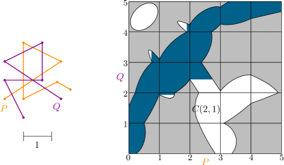
Figure 1: Two polygonal curves $P$ and $Q$, together with their associated free-space diagram. The reachable region $\operatorname{reach}(P,Q)$ is shown in blue. For example, the white area in $C(2,1)$, denoted $F(2,1)$, corresponds to all points on the third edge of $P$ and the second edge of $Q$ that have distance at most $1$. As $(5,5)\in\operatorname{reach}(P,Q)$, we have $d_{F}(P,Q)\leq 1$.

2 Preliminaries and Basic Definitions

Let $P$ and $Q$ be two polygonal curves in the plane, defined by their vertices $p_{0},p_{1},\dots,p_{n}$ and $q_{0},q_{1},\dots,q_{n}$. Depending on the context, we interpret $P$ and $Q$ either as sequences of $n$ and $n$ edges, or as continuous functions $P\colon[0,n]\rightarrow{\mathbb{R}}^{2}$ and $Q\colon[0,n]\rightarrow{\mathbb{R}}^{2}$. In the latter case, we have $P(i+\lambda)=(1-\lambda)p_{i}+\lambda p_{i+1}$ for $i=0,\dots,n-1$ and $\lambda\in[0,1]$, and similarly for $Q$. Let $\Psi$ be the set of all continuous and nondecreasing functions $\alpha\colon[0,1]\rightarrow[0,n]$ with $\alpha(0)=0$ and $\alpha(1)=n$. The Fréchet distance between $P$ and $Q$ is defined as

$$d_{F}(P,Q):=\inf_{\alpha,\beta\in\Psi}\max_{x\in[0,1]}\|P(\alpha(x))-Q(\beta(x))\|,$$

where $\|\cdot\|$ denotes the Euclidean distance.

The classic approach to computing $d_{F}(P,Q)$ uses the free-space diagram $\operatorname{FSD}(P,Q)$. It is defined as

$$\operatorname{FSD}(P,Q):=\{(x,y)\in[0,n]\times[0,n]\mid\|P(x)-Q(y)\|\leq 1\}.$$

In other words, $\operatorname{FSD}(P,Q)$ is the subset of the joint parameter space for $P$ and $Q$ where the corresponding points on the curves have distance at most $1$, see Figure 1.

The structure of $\operatorname{FSD}(P,Q)$ is easy to describe. Let $R:=[0,n]\times[0,n]$ be the ground set. We subdivide $R$ into $n^{2}$ cells $C(i,j)=[i,i+1]\times[j,j+1]$, for $i,j=0,\dots,n-1$. The cell $C(i,j)$ corresponds to the edge pair $e_{i+1}$ and $f_{j+1}$, where $e_{i+1}$ is the $(i+1)$^th edge of $P$ and $f_{j+1}$ is the $(j+1)$^th edge of $Q$. Then the set $F(i,j):=\operatorname{FSD}(P,Q)\cap C(i,j)$ represents all pairs of points on $e_{i+1}\times f_{j+1}$ with distance at most $1$. Elementary geometry shows that $F(i,j)$ is the intersection of $C(i,j)$ with an ellipse [8]. In particular, the set $F(i,j)$ is convex, and the intersection of $\operatorname{FSD}(P,Q)$ with the boundary of $C(i,j)$ consists of four (possibly empty) intervals, one on each side of ${\partial}C(i,j)$. We call these intervals the doors of $C(i,j)$ in $\operatorname{FSD}(P,Q)$. A door is said to be closed if the interval is empty, and open otherwise.

A path $\pi$ in $\operatorname{FSD}(P,Q)$ is bimonotone if it is both $x$- and $y$-monotone, i.e., every vertical and every horizontal line intersects $\pi$ in at most one connected component. Alt and Godau observed that it suffices to decide whether there exists a bimonotone path from $(0,0)$ to $(n,n)$ inside $\operatorname{FSD}(P,Q)$. We define the reachable region $\operatorname{reach}(P,Q)$ as the set of points in $\operatorname{FSD}(P,Q)$ that are reachable from $(0,0)$ on a bimonotone path. Then, $d_{F}(P,Q)\leq 1$ if and only if $(n,n)\in\operatorname{reach}(P,Q)$, see Figure 1. It is not necessary to compute all of $\operatorname{reach}(P,Q)$: since $\operatorname{FSD}(P,Q)$ is convex inside each cell, we only need the intersections $\operatorname{reach}(P,Q)\cap{\partial}C(i,j)$. The sets defined by $\operatorname{reach}(P,Q)\cap{\partial}C(i,j)$ are subintervals of the doors of the free-space diagram, and they are defined by endpoints of doors in the free-space diagram in the same row or column. We call the intersection of a door with $\operatorname{reach}(P,Q)$ a reach-door. The reach-doors can be found in $O(n^{2})$ time through a simple breadth-first-traversal of the cells [8]. In the next sections, we show how to obtain the crucial information, i.e., whether $(n,n)\in\operatorname{reach}(P,Q)$, in $o(n^{2})$ time instead.

Basic approach and intuition

In our algorithm for the decision problem, we basically want to compute $\operatorname{reach}(P,Q)$. But instead of propagating the reachability information cell by cell, we always group $\tau\times\tau$ cells (with $1\ll\tau\ll n$) into an elementary box of cells. When processing a box, we can assume that we know which parts of the left and the bottom boundary of the box are reachable. That is, we know the reach-doors on the bottom and left boundary, and we need to compute the reach-doors on the top and right boundary of the elementary box. These reach-doors are determined by the combinatorial structure of the box. More specifically, suppose we know for every row and column the order of the door endpoints (including for the reach-doors on the left and bottom boundary). Then, we can deduce which of these door boundaries determine the reach-doors on the top and right boundary. We call the sequence of these orders, the (full) signature of the box.

The total number of possible signatures is bounded by an expression in terms of $\tau$. Thus, if we pick $\tau$ sufficiently small compared to $n$, we can pre-compute for all possible signatures the reach-doors on the top and right boundary, and build a data structure to query these quickly (Section 3). Since the reach-doors on the bottom and left boundary are required to make the signature, we initially have only incomplete signatures. In Section 4, we describe how to compute these efficiently. The incomplete signatures are then used to preprocess the data structure such that we can quickly find the full signature once we know the reach-doors of an elementary box. After building and preprocessing the data structure, it is possible to determine $d_{F}(P,Q)\leq 1$ efficiently by traversing the free-space diagram elementary box by elementary box, as explained in Section 5.

3 Building a Lookup Table

3.1 Preprocessing an elementary box

Before it considers the input, our algorithm builds a lookup table. As mentioned above, the purpose of this table is to speed up the computation of small parts of the free-space diagram.

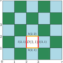
Figure 2: The elementary box. The cell $D(2,1)$ is shown white. Its boundaries—$l(2,1)$, $l(3,1)$, $b(2,1)$, $b(2,2)$—are indicated.

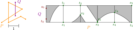
Figure 3: The door-order of a row (the vertical order of the points) encodes the combinatorial structure of the doors. The door-order for the row in the figure is $s_{1}s_{3}s_{4}t_{5}t_{3}t_{0}s_{2}t_{4}s_{0}s_{5}t_{1}t_{2}$. Note that $s_{0}$ and $t_{0}$ represent the reach-door, which is empty in this case. These are omitted in the incomplete door-order.

Let $\tau\in\mathbb{N}$ be a parameter. The elementary box is a subdivision of $[0,\tau]^{2}$ into $\tau$ columns and rows, thus $\tau^{2}$ cells. For $i,j=0,\dots,\tau-1$, we denote the cell $[i,i+1]\times[j,j+1]$ with $D(i,j)$. We denote the left side of the boundary ${\partial}D(i,j)$ by $l(i,j)$ and the bottom side by $b(i,j)$. Note that $l(i,j)$ coincides with the right side of ${\partial}D(i-1,j)$ and $b(i,j)$ with the top of ${\partial}D(i,j-1)$. Thus, we write $l(\tau,j)$ for the right side of $D(\tau-1,j)$ and $b(i,\tau)$ for the top side of $D(i,\tau-1)$. Figure 2 shows the elementary box.

The door-order $\sigma_{j}^{r}$ for a row $j$ is a permutation of $\{s_{0},t_{0},\dots,s_{\tau},t_{\tau}\}$, having $2\tau+2$ elements. For $i=1,\dots,\tau$, the element $s_{i}$ represents the lower endpoint of the door on $l(i,j)$, and $t_{i}$ represents the upper endpoint. The elements $s_{0}$ and $t_{0}$ are an exception: they describe the reach-door on the boundary $l(0,j)$ (i.e., its intersection with $\operatorname{reach}(P,Q)$). The door-order $\sigma_{j}^{r}$ represents the combinatorial order of these endpoints, as projected onto a vertical line, i.e., they are sorted into their vertical order. Some door-orders may encode the same combinatorial structure. In particular, when door $i$ is closed, the exact position of $s_{i}$ and $t_{i}$ in a door-order is irrelevant, as long as $t_{i}$ comes before $s_{i}$. For a closed door $i$ ($i>0$), we assign $s_{i}$ to the upper endpoint of $l(i,j)$ and $t_{i}$ to the lower endpoint. The values of $s_{0}$ and $t_{0}$ are defined by the reach-door and their relative order is thus a result of computation. We break ties between $s_{i}$ and $t_{i^{\prime}}$ by placing $s_{i}$ before $t_{i^{\prime}}$, and any other ties are resolved by index. A door-order $\sigma_{i}^{c}$ is defined analogously for a column $i$. We write $x<_{i}^{c}y$ if $x$ comes before $y$ in $\sigma_{i}^{c}$, and $x<_{j}^{r}y$ if $x$ comes before $y$ in $\sigma_{j}^{r}$. An incomplete door-order is a door-order in which $s_{0}$ and $t_{0}$ are omitted (i.e. the intersection of $\operatorname{reach}(P,Q)$ with the door is still unknown); see Figure 3.

We can now define the (full) signature of the elementary box as the aggregation of the door-orders of its rows and columns. Therefore, a signature $\Sigma=(\sigma_{1}^{c},\dots,\sigma_{\tau}^{c},\sigma_{1}^{r},\dots,\sigma_{\tau}^{r})$ consists of $2\tau$ door-orders: one door-order $\sigma_{i}^{c}$ for each column $i$ and one door-order $\sigma_{j}^{r}$ for each row $j$ of the elementary box. Similarly, an incomplete signature is the aggregation of incomplete door-orders.

For a given signature, we define the combinatorial reachability structure of the elementary box as follows. For each column $i$ and for each row $j$, the combinatorial reachability structure indicates which door boundaries in the respective column or row define the reach-door of $b(i,\tau)$ or $l(\tau,j)$.

Lemma 3.1.

Let $\Sigma$ be a signature for the elementary box. Then we can determine the combinatorial reachability structure of the box in total time $O(\tau^{2})$.

Proof.

We use dynamic programming, very similar to the algorithm by Alt and Godau [8]. For each vertical edge $l(i,j)$ we define a variable $\widehat{l}(i,j)$, and for each horizontal edge $b(i,j)$ we define a variable $\widehat{b}(i,j)$. The $\widehat{l}(i,j)$ are pairs of the form $(s_{u},t_{v})$, representing the reach-door $\operatorname{reach}(P,Q)\cap l(i,j)$. If this reach-door is closed, then $t_{v}<_{j}^{r}s_{u}$ holds. If the reach-door is open, then it is bounded by the lower endpoint of the door on $l(u,j)$ and by the upper endpoint of the door on $l(v,j)$. (Note that in this case we have $v=i$.) Once again $s_{0}$ and $t_{0}$ are special and represent the reach-door on $l(0,j)$. The variables $\widehat{b}(i,j)$ are defined analogously.

Now we can compute $\widehat{l}(i,j)$ and $\widehat{b}(i,j)$ recursively as follows: first, we set

$$\widehat{l}(0,j)=\widehat{b}(i,0)=(s_{0},t_{0}),\quad\textnormal{for }i,j=0,\dots,\tau-1.$$

Next, we describe how to find $\widehat{l}(i,j)$ given $\widehat{l}(i-1,j)$ and $\widehat{b}(i-1,j)$, see Figure 4.

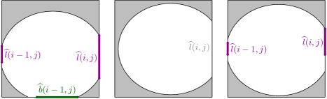
Figure 4: The three cases for the recursive definition of $\widehat{l}(i,j)$. If the lower boundary is reachable, we can reach the whole right door (left). If neither the lower nor the left boundary is reachable, the right door is not reachable either (middle). Otherwise, the lower boundary is the maximum of $\widehat{l}(i-1,j)$ and the lower boundary of the right door (right).

Case 1: Suppose $\widehat{b}(i-1,j)$ is open. This means that $b(i-1,j)$ intersects $\operatorname{reach}(P,Q)$, so $\operatorname{reach}(P,Q)\cap l(i,j)$ is limited only by the door on $l(i,j)$, and we can set $\widehat{l}(i,j):=(s_{i},t_{i})$.

Case 2: If both $\widehat{b}(i-1,j)$ and $\widehat{l}(i-1,j)$ are closed, it is impossible to reach $l(i,j)$ and thus we set $\widehat{l}(i,j):=\widehat{l}(i-1,j)$.

Case 3: If $\widehat{b}(i-1,j)$ is closed and $\widehat{l}(i-1,j)$ is open, we may be able to reach $l(i,j)$ via $l(i-1,j)$. Let $s_{u}$ be the lower endpoint of $\widehat{l}(i-1,j)$. We need to pass $l(i,j)$ above $s_{u}$ and $s_{i}$ and below $t_{i}$, and therefore set $\widehat{l}(i,j):=(\max(s_{u},s_{i}),t_{i})$, where the maximum is taken according to the order $<_{j}^{r}$.

The recursion for the variable $\widehat{b}(i,j)$ is defined similarly. We can implement the recursion in time $O(\tau^{2})$ for any given signature, for example by traversing the elementary box column by column, while processing each column from bottom to top. ∎

There are at most $((2\tau+2)!)^{2\tau}=\tau^{O(\tau^{2})}$ distinct signatures for the elementary box. We choose $\tau=\lambda\sqrt{\log n/\log\log n}$ for a sufficiently small constant $\lambda>0$, so that this number becomes $o(n)$. Thus, during the preprocessing stage we have time to enumerate all possible signatures and determine the corresponding combinatorial reachability structure inside the elementary box. This information is then stored in an appropriate data structure.

3.2 Building the data structure

Before we describe this data structure, we first explain how the door-orders are represented. This depends on the computational model. By our choice of $\tau$, there are $o(n)$ distinct door-orders. On the word RAM, we represent each door-order and incomplete door-order by an integer between $1$ and $(2\tau)!$. This fits into a word of $\log n$ bits. On the pointer machine, we create a record for each door-order and incomplete door-order; we represent an order by a pointer to the corresponding record.

The data structure has two stages. In the first stage, we assume we know the incomplete door-order for each row and for each column of the elementary box, and we wish to determine the incomplete signature. In the second stage we have obtained the reach-doors for the left and bottom sides of the elementary box, and we are looking for the full signature. The details of our method depend on the computational model. One way uses table lookup and requires the word RAM; the other way works on the pointer machine, but is a bit more involved.

Word RAM

We organize the lookup table as a large tree $T$. In the first stage, each level of $T$ corresponds to a row or column of the elementary box. Thus, there are $2\tau$ levels. Each node has $(2\tau)!$ children, representing the possible incomplete door-orders for the next row or column. Since we represent door-orders by positive integers, each node of $T$ may store an array for its children; we can choose the appropriate child for a given incomplete door-order in constant time. Thus, determining the incomplete signature for an elementary box requires $O(\tau)$ steps on a word RAM.

For the second stage, we again use a tree structure. Now the tree has $O(\tau)$ layers, each with $O(\log\tau)$ levels. Again, each layer corresponds to a row or column of the elementary box. The levels inside each layer then implement a balanced binary search tree that allows us to locate the endpoints of the reach-door within the incomplete signature. Since there are $2\tau$ endpoints, this requires $O(\log\tau)$ levels. Thus, it takes $O(\tau\log\tau)$ time to find the full signature of a given elementary box.

Pointer machine

Unlike in the word RAM model, we are not allowed to store a lookup table on every level of the tree $T$, and there is no way to quickly find the appropriate child for a given door-order. Instead, we must rely on batch processing to achieve a reasonable running time.

Thus, suppose that during the first stage we want to find the incomplete signatures for a set $B$ of $m$ elementary boxes, where again for each box in $B$ we know the incomplete door-order for each row and each column. Recall that we represent the door-order by a pointer to the corresponding record. With each such record, we store a queue of elementary boxes that is empty initially.

We now simultaneously propagate the boxes in $B$ through $T$, proceeding level by level. In the first level, all of $B$ is assigned to the root of $T$. Then, we go through the nodes of one level of $T$, from left to right. Let $v$ be the current node of $T$. We consider each elementary box $b$ assigned to $v$. We determine the next incomplete door-order for $b$, and we append $b$ to the queue for this incomplete door-order—the queue is addressed through the corresponding record, so all elementary boxes with the same next incomplete door-order end up in the same queue. Next, we go through the nodes of the next level, again from left to right. Let $v^{\prime}$ be the current node. The node $v^{\prime}$ corresponds to a next incomplete door-order $\sigma$ that extends the known signature of its parents. We consider the queue stored at the record for $\sigma$. By construction, the elementary boxes that should be assigned to $v^{\prime}$ appear consecutively at the beginning of this queue. We remove these boxes from the queue and assign them to $v^{\prime}$. After this, all the queues are empty, and we can continue by propagating the boxes to the next level. During this procedure, we traverse each node of $T$ a constant number of times, and in each level of the $T$ we consider all the boxes in $B$. Since $T$ has $o(n)$ nodes, the total running time is $O(n+m\tau)$.

For the second stage, the data structure works just as in the word RAM case, because no table lookup is necessary. Again, we need $O(\tau\log\tau)$ steps to process one box. After the second stage, we obtain the combinatorial reachability structure of the box in constant time since we precomputed this information for each box (Lemma 3.1). Thus, we have shown the following lemma, independently of the computational model.

Lemma 3.2.

For $\tau=\lambda\sqrt{\log n/\log\log n}$, with a sufficiently small constant $\lambda>0$, we can construct in $o(n)$ time a data structure of size $o(n)$ such that

• given a set of $m$ elementary boxes where the incomplete door-orders are known, we can find the incomplete signature of each box in total time $O(n+m\tau)$;

• given the incomplete signature and the reach-doors on the bottom and left boundary of an elementary box, we can find the full signature in $O(\tau\log\tau)$ time;

• given the full signature of an elementary box, we can find the combinatorial reachability structure of the box in constant time.

4 Preprocessing a Given Input

Next, we perform a second preprocessing phase that considers the input curves $P$ and $Q$. Our eventual goal is to compute the intersection of $\operatorname{reach}(P,Q)$ with the cell boundaries, taking advantage of the data structure from Section 3. For this, we aggregate the cells of $\operatorname{FSD}(P,Q)$ into (concrete) elementary boxes consisting of $\tau\times\tau$ cells. There are $n^{2}/\tau^{2}$ such boxes. We may avoid rounding issues by either duplicating vertices or handling a small part of $\operatorname{FSD}(P,Q)$ without lookup tables.

The goal is to determine the signature for each elementary box $S$. At this point, this is not quite possible yet, since the signature depends on the intersection of $\operatorname{reach}(P,Q)$ with the lower and left boundary of $S$. Nonetheless, we can find the incomplete signature, in which the positions of $s_{0},t_{0}$ (the reach-door) in the (incomplete) door-orders $\sigma_{i}^{r}$, $\sigma_{j}^{c}$ are still to be determined.

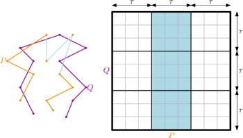
Figure 5: $\operatorname{FSD}(P,Q)$ is subdivided into $n^{2}/\tau^{2}$ elementary boxes of size $\tau\times\tau$. The free-space diagram is subdivided into $n^{2}/\tau^{2}$ elementary boxes of size $\tau\times\tau$. A strip is a column of elementary boxes: it corresponds to a subcurve of $P$ with $\tau$ edges.

We aggregate the columns of $\operatorname{FSD}(P,Q)$ into vertical strips, each corresponding to a single column of elementary boxes (i.e., $\tau$ consecutive columns of cells in $\operatorname{FSD}(P,Q)$). See Figure 5.

Let $A$ be such a strip. It corresponds to a subcurve $P^{\prime}$ of $P$ with $\tau$ edges. The following lemma implies that we can build a data structure for $A$ such that, given any segment of $Q$, we can efficiently find its incomplete door-order within the elementary box in $A$.

Lemma 4.1.

Given a subcurve $P^{\prime}$ with $\tau$ edges, we can compute in $O(\tau^{6})$ time a data structure that requires $O(\tau^{6})$ space and that allows us to determine the incomplete door-order of any line segment on $Q$ in time $O(\log\tau)$.

Proof.

Consider the arrangement $\mathcal{A}$ of unit circles whose centers are the vertices of $P^{\prime}$ (see Figure 6). The incomplete door-order of a line segment $s$ is determined by the intersections of $s$ with the arcs of $\mathcal{A}$ (and for a circle not intersecting $s$ by whether $s$ lies inside or outside of the circle). Let $\ell_{s}$ be the line spanned by line segment $s$. Suppose we wiggle $\ell_{s}$. The order of intersections of $\ell_{s}$ and the arcs of $\mathcal{A}$ changes only when $\ell_{s}$ moves over a vertex of $\mathcal{A}$ or if $\ell_{s}$ leaves or enters a circle.

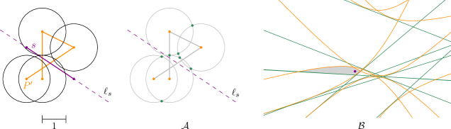
Figure 6: By using the arrangement $\mathcal{A}$ defined by unit circles centered at vertices of $P^{\prime}$, we can determine the incomplete door-order of each segment $s$ on $Q$. This is done by locating the dual point of $\ell_{s}$ in the dual arrangement $\mathcal{B}$. The dual arrangement also contains pseudolines to determine when $\ell_{s}$ leaves a circle of $\mathcal{A}$.

We use the standard duality transform that maps a line $\ell:y=ax+b$ to the point $\ell^{*}:(a,-b)$, and vice versa. Consider a unit circle $C$ in $\mathcal{A}$ with center $(c_{x},c_{y})$. Elementary geometry shows that the set of all lines that are tangent to $C$ from above dualizes to the curve $t_{a}^{*}(C):y=c_{x}x-c_{y}-\sqrt{1+x^{2}}$. Similarly, the lines that are tangent to $C$ from below dualize to the curve $t_{b}^{*}(C):y=c_{x}x-c_{y}+\sqrt{1+x^{2}}$. Define $C^{*}:=\{t_{a}^{*}(C),t_{b}^{*}(C)\mid C\in\mathcal{A}\}$. Since any pair of distinct circles $C_{1}$, $C_{2}$ has at most four common tangents, one for each choice of above/below $C_{1}$ and above/below $C_{2}$, it follows that any two curves in $C^{*}$ intersect at most once.

Let $V$ be the set of vertices in $\mathcal{A}$, and let $V^{*}$ be the lines dual to the points in $V$ (note that $|V|=O(\tau^{2})$). Since for any vertex $v\in V$ and any circle $C\in\mathcal{A}$ there are at most two tangents through $v$ on $C$, each line in $V^{*}$ intersects each curve in $C^{*}$ at most once. Thus, the arrangement $\mathcal{B}$ of the curves in $V^{*}\cup C^{*}$ is an arrangement of pseudolines with complexity $O(\tau^{4})$. Furthermore, it can be constructed in the same expected time, together with a point location structure that finds the containing cell in $\mathcal{B}$ of any given point in time $O(\log\tau)$ [60, Chapter 6.6.1].

Now consider a line segment $s$ and the supporting line $\ell_{s}$. As observed in the first paragraph, the combinatorial structure of the intersection between $\ell_{s}$ and $\mathcal{A}$ is completely determined by the cell of $\mathcal{B}$ that contains the dual point $\ell_{s}^{*}$. Thus, for every cell $f(s)\in\mathcal{B}$, we construct a list $L_{f(s)}$ that represents the combinatorial structure of $\ell_{s}\cap\mathcal{A}$. There are $O(\tau^{4})$ such lists, each having size $O(\tau)$. We can compute $L_{f(s)}$ by traversing the zone of $\ell_{s}$ in $\mathcal{A}$. Since circles intersect at most twice and since a line intersects any circle at most twice, the zone has complexity $O(\tau 2^{\alpha(\tau)})$, where $\alpha(\cdot)$ denotes the inverse Ackermann function [60, Theorem 5.11]. Since $O(\tau 2^{\alpha(\tau)})\subset O(\tau^{2})$, we can compute all lists in $O(\tau^{6})$ time.

Given the list $L_{f(s)}$, the incomplete door-order of $s$ is determined by the position of the endpoints of $s$ in $L_{f(s)}$. There are $O(\tau^{2})$ possible ways for this, and we build a table $T_{f(s)}$ that represents them. For each entry in $T_{f(s)}$, we store a representative for the corresponding incomplete door-order. As described in the previous section, the representative is a positive integer in the word RAM model and a pointer to the appropriate record on a pointer machine.

The total size of the data structure is $O(\tau^{6})$ and it can be constructed in the same time. A query works as follows: given $s$, we can compute $\ell_{s}^{*}$ in constant time. Then we use the point location structure of $\mathcal{B}$ to find $f(s)$ in $O(\log\tau)$ time. Using binary search on $T_{f(s)}$ (or an appropriate tree structure in the case of a point machine), we can then determine the position of the endpoints of $s$ in the list $L_{f(s)}$ in $O(\log\tau)$ time. This bound holds both on the word RAM and on the pointer machine. ∎

Lemma 4.2.

Given the data structure of Lemma 3.2, the incomplete signature for each elementary box can be determined in time $O(n\tau^{5}+n^{2}(\log\tau)/\tau)$.

Proof.

By building and using the data structure from Lemma 4.1, we determine the incomplete door-order for each row in each vertical $\tau$-strip in total time proportional to

$$\frac{n}{\tau}(\tau^{6}+n\log\tau)=n\tau^{5}+\frac{n^{2}\log\tau}{\tau}.$$

We repeat the procedure with the horizontal strips. Now we know for each elementary box in $\operatorname{FSD}(P,Q)$ the incomplete door-order for each row and each column. We use the data structure of Lemma 3.2 to combine these. As there are $n^{2}/\tau^{2}$ boxes, the number of steps is $O(n^{2}/\tau+n)=O(n^{2}/\tau)$. Hence, the incomplete signature for each elementary box is found in $O(n\tau^{5}+n^{2}(\log\tau)/\tau)$ steps. ∎

5 Solving the Decision Problem

With the data structures and preprocessing from the previous sections, we have all ingredients in place to determine whether $d_{F}(P,Q)\leq 1$. We know for each elementary box its incomplete signature and we have a data structure to derive its full signature (and with it, the combinatorial reachability structure) when its reach-doors are known. What remains to be shown is that we can efficiently process the free-space diagram to determine whether $(n,n)\in\operatorname{reach}(P,Q)$. This is captured in the following lemma.

Lemma 5.1.

If the incomplete signature for each elementary box is known, we can determine whether $(n,n)\in\operatorname{reach}(P,Q)$ in time $O(n^{2}(\log\tau)/\tau)$.

Proof.

We go through all elementary boxes of $\operatorname{FSD}(P,Q)$, processing them one column at a time, going from bottom to top in each column. Initially, we know the full signature for the box $S$ in the lower left corner of $\operatorname{FSD}(P,Q)$. We use the signature to determine the intersections of $\operatorname{reach}(P,Q)$ with the upper and right boundary of $S$. There is a subtlety here: the signature gives us only the combinatorial reachability structure, and we need to map the resulting $s_{i},t_{j}$ back to the corresponding vertices on the curves. On the word RAM, this can be done easily through table lookups. On the pointer machine, we use representative records for the $s_{i},t_{i}$ elements and use $O(\tau)$ time before processing the box to store a pointer from each representative record to the appropriate vertices on $P$ and $Q$.

We proceed similarly for the other boxes. By the choice of the processing order of the elementary boxes we always know the incoming reach-doors on the bottom and left boundary when processing a box. Given the incoming reach-doors, we can determine the full signature and find the structure of the outgoing reach-doors in total time $O(\tau\log\tau)$, using Lemma 3.2. Again, we need $O(\tau)$ additional time on the pointer machine to establish the mapping from the abstract $s_{i}$, $t_{i}$ elements to the concrete vertices of $P$ and $Q$. In total, we spend $O(\tau\log\tau)$ time per box. Thus, it takes time $O(n^{2}(\log\tau)/\tau)$ to process all boxes, as claimed. ∎

As a result, we obtain the following theorem for the pointer machine (and, by extension, for the real RAM model). For the word RAM model, we can obtain an even faster algorithm (see Section 6).

Theorem 5.2.

There is an algorithm that solves the decision version of the Fréchet problem in $O(n^{2}(\log\log n)^{3/2}/\sqrt{\log n})$ time on a pointer machine.

Proof.

Set $\tau=\lambda\sqrt{\log n/\log\log n}$, for a sufficiently small constant $\lambda>0$. The theorem follows by applying Lemmas 3.2, 4.2, and 5.1 in sequence. ∎

6 Improved Bound on the Word RAM

We now explain how the running time of our algorithm can be improved if our computational model allows for constant time table-lookup. We use the same $\tau$ as above (up to a constant factor). However, we change a number of things. “Signatures” are represented differently and the data structure to obtain combinatorial reachability structures is changed accordingly. Furthermore, we aggregate elementary boxes into clusters and determine “incomplete door-orders” for multiple boxes at the same time. Finally, we walk the free-space diagram based on the clusters to decide $d_{F}(P,Q)\leq 1$.

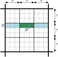
Figure 7: A cluster consists of $\tau\times\tau$ elementary boxes, thus of $\tau^{2}\times\tau^{2}$ cells. A row $R$ and its corresponding $R^{\prime}$ for the central elementary box are indicated.

Clusters and extended signatures

We introduce a second level of aggregation in the free-space diagram (see Figure 7): a cluster is a collection of $\tau\times\tau$ elementary boxes, that is, $\tau^{2}\times\tau^{2}$ cells in $\operatorname{FSD}(P,Q)$. Let $R$ be a row of cells in $\operatorname{FSD}(P,Q)$ of a certain cluster. As before, the row $R$ corresponds to an edge $e$ on $Q$ and a subcurve $P^{\prime}$ of $P$ with $\tau^{2}$ edges. We associate with $R$ an ordered set $Z=\langle e_{0},z_{0}^{\prime},z_{1},z_{1}^{\prime},z_{2},z_{2}^{\prime},\dots,z_{k},z_{k}^{\prime},e_{1}\rangle$ with $2\cdot k+3$ elements. Here $k$ is the number of intersections of $e$ with the unit circles centered at the $\tau^{2}$ vertices of $P^{\prime}$ (all but the very first). Hence, $k$ is bounded by $2\tau^{2}$ and $|Z|$ is bounded by $4\tau^{2}+3$. The order of $Z$ indicates the order of these intersections with $e$ directed along $Q$. Elements $e_{0}$ and $e_{1}$ represent the endpoints of $e$ and take a special role. In particular, these are used to represent closed doors and snap open doors to the edge $e$. The elements $z_{i}^{\prime}$ are placeholders for the positions of the endpoints of the reach-doors: $z_{0}^{\prime}$ represents a possible reach-door endpoint between $e_{0}$ and $z_{1}$, the element $z_{1}^{\prime}$ represents an endpoint between $z_{1}$ and $z_{2}$, etc.

Consider a row $R^{\prime}$ of an elementary box inside the row $R$ of a cluster, corresponding to an edge $e$ of $Q$. The door-index of $R^{\prime}$ is an ordered set $\langle s_{0},t_{0},\ldots,s_{\tau},t_{\tau}\rangle$ of size $2\tau+2$. Similar to a door-order, elements $s_{0}$ and $t_{0}$ represent the reach-door at the leftmost boundary of $R^{\prime}$; the elements $s_{i}$ and $t_{i}$ ($1\leq i\leq\tau$) represent the door at the right boundary of the $i$^th cell in $R^{\prime}$. However, instead of rearranging the set to indicate relative positions, the elements $s_{i}$ and $t_{i}$ simply refer to elements in $Z$. If the door is open, they refer to the corresponding intersections with $e$ (possibly snapped to $e_{0}$ or $e_{1}$). If the door is closed, $s_{i}$ is set to $e_{1}$ and $t_{i}$ is set to $e_{0}$. The elements $s_{0}$ and $t_{0}$ are special, representing the reach-door, and they refer to one of the elements $z_{i}^{\prime}$. An incomplete door-index is a door-index without $s_{0}$ and $t_{0}$. The advantage of a door-index over a door-order is that the reach-door is always at the start. Hence, completing an incomplete door-index to a full door-index can be done in constant time. Since a door-index has size $2\tau+2$, the number of possible door-indices for $R^{\prime}$ is $\tau^{O(\tau)}$.

We define the door-indices for the columns analogously. We concatenate the door-indices for the rows and the columns to obtain the indexed signature for an elementary box. Similarly, we define the incomplete indexed signature. The total number of possible indexed signatures remains $\tau^{O(\tau^{2})}$.

For each possible incomplete indexed signature $\Sigma$ we build a lookup table $T_{\Sigma}$ as follows: the input is a word with $4\tau$ fields of $O(\log\tau)$ bits each. Each field stores the positions in $Z$ of the endpoints of the ingoing reach-doors for the elementary box: $2\tau$ fields for the left side, $2\tau$ fields for the lower side. The output consists of a word that represents the indices for the elements in $Z$ that represent the outgoing reach-doors for the upper and right boundary of the box. Thus, the input of $T_{\Sigma}$ is a word of $O(\tau\log\tau)$ bits, and $T_{\Sigma}$ has size $\tau^{O(\tau)}$. Hence, for all incomplete indexed signatures combined, the size is $\tau^{O(\tau^{2})}=o(n)$ by our choice of $\tau$.

Preprocessing a given input

During the preprocessing for a given input $P,Q$, we use superstrips consisting of $\tau$ strips. That is, a superstrip is a column of clusters and consists of $\tau^{2}$ columns of the free-space diagram. Lemma 4.1 still holds, albeit with a larger constant $c$ in place of $6$. The data structure gets as input a query edge $e$, and it returns in $O(\log\tau)$ time a word that contains $\tau$ fields. Each field represents the incomplete door-index for $e$ in the corresponding elementary box and thus consists of $O(\tau\log\tau)$ bits. Hence, the word size is $O(\tau^{2}\log\tau)=O(\log n)$ by our choice of $\tau$. Thus, the total time for building a data structure for each superstrip and for processing all rows is $O(n/\tau^{2}\;(\tau^{c}+n\log\tau))=O(n^{2}(\log\tau)/\tau^{2})$. We now have parts of the incomplete indexed signature for each elementary box packed into different words. To obtain the incomplete indexed signature, we need to rearrange the information such that the incomplete door-indices of the rows in one elementary box are in a single word. This corresponds to computing a transpose of a matrix, as is illustrated in Figure 8. For this, we need the following lemma, which can be found—in slightly different form—in Thorup [62, Lemma 9].

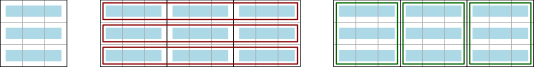
Figure 8: (left) Every field represents the incomplete door-index of a row in an elementary box. (center) The fields are grouped into words per row in a cluster. (right) Transposition yields the desired organization, where a word represents the incomplete door-index of the rows in an elementary box.

Lemma 6.1.

Let $X$ be a sequence of $\tau$ words that contain $\tau$ fields each, so that $X$ can be interpreted as a $\tau\times\tau$ matrix. Then we can compute in time $O(\tau\log\tau)$ on a word RAM a sequence $Y$ of $\tau$ words with $\tau$ fields each that represents the transpose of $X$.

Proof.

The algorithm is recursive and solves a more general problem: let $X$ be a sequence of $a$ words that represents a sequence $M$ of $b$ different $a\times a$ matrices, such that the $i$^th word in $X$ contains the fields of the $i$^th row of each matrix in $M$ from left to right. Compute a sequence of words $Y$ that represents the sequence $M^{\prime}$ of the transposed matrices in $M$.

The recursion works as follows: if $a=1$, there is nothing to be done. Otherwise, we split $X$ into the sequence $X_{1}$ of the first $a/2$ words and the sequence $X_{2}$ of the remaining words. $X_{1}$ and $X_{2}$ now represent a sequence of $2b$ $(a/2)\times(a/2)$ matrices, which we transpose recursively. After the recursion, we put the $(a/2)\times(a/2)$ submatrices back together in the obvious way. To finish, we need to transpose the off-diagonal submatrices. This can be done simultaneously for all matrices in time $O(a)$, by using appropriate bit-operations (or table lookup). Hence, the running time obeys a recursion of the form $T(a)=2T(a/2)+O(a)$, giving $T(a)=O(a\log a)$, as desired. ∎

By applying the lemma to the words that represent $\tau$ consecutive rows in a superstrip, we obtain the incomplete door-indices of the rows for each elementary box. This takes total time proportional to

$$\frac{n}{\tau^{2}}\cdot\frac{n}{\tau}\cdot\tau\log\tau=\frac{n^{2}}{\tau^{2}}\log\tau.$$

We repeat this procedure for the horizontal superstrips. By using an appropriate lookup table to combine the incomplete door-indices of the rows and columns, we obtain the incomplete indexed signature for each elementary box in total time $O(n^{2}(\log\tau)/\tau^{2})$.

The actual computation

We traverse the free-space diagram cluster by cluster (recall that a cluster consists of $\tau\times\tau$ elementary boxes). The clusters are processed column by column from left to right, and inside each column from bottom to top. Before processing a cluster, we walk along the left and lower boundary of the cluster to determine the incoming reach-doors. This is done by performing a binary search for each box on the boundary, and determining the appropriate elements $z_{i}^{\prime}$ which correspond to the incoming reach-doors. Using this information, we assemble the appropriate words that represent the incoming information for each elementary box. Since there are $n^{2}/\tau^{4}$ clusters, this step requires time $O((n^{2}/\tau^{4})\tau^{2}\log\tau)=O(n^{2}(\log\tau)/\tau^{2})$. We then process the elementary boxes inside the cluster, in a similar fashion. Now, however, we can process each elementary box in constant time through a single table lookup, so the total time is $O(n^{2}/\tau^{2})$. Hence, the total running time of our algorithm is $O(n^{2}(\log\tau)/\tau^{2})$. By our choice of $\tau=\lambda\sqrt{\log n/\log\log n}$ for a sufficiently small $\lambda>0$, we obtain the following theorem.

Theorem 6.2.

The decision version of the Fréchet problem can be solved in $O(n^{2}(\log\log n)^{2}/\log n)$ time on a word RAM.

7 Computing the Fréchet Distance

The optimization version of the Fréchet problem, i.e., computing the Fréchet distance, can be done in $O(n^{2}\log n)$ time using parametric search with the decision version as a subroutine [8]. We showed that the decision problem can be solved in $o(n^{2})$ time. However, this does not directly yield a faster algorithm for the optimization problem: if the running time of the decision problem is $T(n)$, parametric search gives an $O((T(n)+n^{2})\log n)$ time algorithm [8]. There is an alternative randomized algorithm by Raichel and Har-Peled [49]. Their algorithm also needs $O((T(n)+n^{2})\log n)$ time, but below we adapt it to obtain the following lemma.

Lemma 7.1.

The Fréchet distance of two polygonal curves with $n$ vertices each can be computed by a randomized algorithm in $O(n^{2}2^{\alpha(n)}+T(n)\log n)$ expected time, where $T(n)$ is the time for the decision problem.

Before we prove the lemma, we recall that possible values of the Fréchet distance are limited to a certain set of critical values [8]:

1. the distance between a vertex of one curve and a vertex of the other curve (vertex-vertex);

2. the distance between a vertex of one curve and an edge of the other curve (vertex-edge); and

3. for two vertices of one curve and an edge of the other curve, the distance between one of the vertices and the intersection of $e$ with the bisector of the two vertices (if this intersection exists) (vertex-vertex-edge).

If we also include vertex-vertex-edge tuples with no intersection, we can sample a critical value uniformly at random in constant time. The algorithm now works as follows (see Har-Peled and Raichel [49] for more details): first, we sample a set $S$ of $K=4n^{2}$ critical values uniformly at random. Next, we find $a^{\prime},b^{\prime}\in S$ such that the Fréchet distance lies between $a^{\prime}$ and $b^{\prime}$ and such that $[a^{\prime},b^{\prime}]$ contains no other value from $S$. In the original algorithm this is done by sorting $S$ and performing a binary search using the decision version. Using median-finding instead, this step can be done in $O(K+T(n)\log K)$ time. Alternatively, the running time of this step could be reduced by picking a smaller $K$. However, this does not improve the final bound, since it is dominated by a $O(n^{2}2^{\alpha(n)})$ term. The interval $[a^{\prime},b^{\prime}]$ with high probability contains only a small number of the remaining critical values. More precisely, for $K=4n^{2}$ the probability that $[a^{\prime},b^{\prime}]$ has more than $2cn\ln n$ critical values is at most $1/n^{c}$ [49, Lemma 6.2].

The remainder of the algorithm proceeds as follows: first, we find all critical values of type vertex-vertex and vertex-edge that lie inside the interval $[a^{\prime},b^{\prime}]$. This can be done in $O(n^{2})$ time by checking all vertex-vertex and vertex-edge pairs. Among these values, we again use median-finding to determine the interval $[a,b]\subseteq[a^{\prime},b^{\prime}]$ that contains the Fréchet distance in $O(K^{\prime}+T(n)\log K^{\prime})$ time. It remains to determine the critical values corresponding to vertex-vertex-edge tuples that lie in $[a,b]$.

For this, take an edge $e$ of $P$ and the vertices of $Q$. Conceptually, we start with circles of radius $a$ around the vertices of $Q$, and we increase the radii until $b$. During this process, we observe the evolution of the intersection points between the circle arcs and $e$. Because all vertex-vertex and vertex-edge events have been eliminated, each circle intersects $e$ in either $0$ or $2$ points, and this does not change throughout the process. A critical value of vertex-vertex-edge type corresponds to the event that two different circles intersect $e$ in the same point, i.e., that two intersection points meet while growing the circles. Two intersection points can meet at most once, and when they do, they exchange their order along $e$.

This suggests the following algorithm: let $\mathcal{A}_{a}$ be the arrangement of circles with radius $a$ around the vertices of $Q$, and let $\mathcal{A}_{b}$ be the concentric arrangement of circles with radius $b$. We determine the ordered sequence $I_{a}$ of the intersection points of the circles in $\mathcal{A}_{a}$ with $e$, and we number them in their order along $e$. Next, we find the ordered sequence of intersection points $I_{b}$ between $e$ and the circles in $\mathcal{A}_{b}$. We assign to each point in $I_{b}$ the number of the corresponding intersection points in $I_{a}$. Since $|I_{a}|=|I_{b}|$, this gives a permutation of $\{1,\dots,|I_{a}|\}$, Two intersection points change their order from $I_{a}$ to $I_{b}$ exactly if there is a vertex-vertex-edge event in $[a,b]$, so these events correspond to the inversions of the resulting permutation. Given that there are $k$ such inversions, we can find them in time $O(|I_{a}|+k)$ using insertion sort. Thus, the overall running time to find the critical events in $[a,b]$, ignoring the time for computing $I_{a}$ and $I_{b}$, is $O(n^{2}+K^{\prime})$.

It remains to show that we can quickly find $I_{a}$ and $I_{b}$. We describe the algorithm for $I_{a}$. First, compute the arrangement $\mathcal{A}_{a}$ of circles with radius $a$ around the vertices of $Q$. This takes $O(n^{2})$ time [33]. To find the intersection order, traverse in $\mathcal{A}_{a}$ the zone of the line $\ell$ spanned by $e$. The time for the traversal is bounded by the complexity of the zone. Since the circles pairwise intersect at most twice and $\ell$ intersects each circle only twice, the complexity of the zone is $O(n2^{\alpha(n)})$ [60, Theorem 5.11]. Summing over all edges $e$, this adds a total of $O(n^{2}2^{\alpha(n)})$ to the running time. To find $I_{b}$, we proceed similarly with $\mathcal{A}_{b}$. Thus the overall time is $O(T(n)\log(n)+n^{2}2^{\alpha(n)}+K^{\prime})$. The event $K^{\prime}>8n\ln n$ has probability less than $1/n^{4}$, and we always have $K^{\prime}=O(n^{3})$. Thus, this case adds $o(1)$ to the expected running time. Given $K^{\prime}\leq 8n\ln n$, the running time is $O(n\log n)$. Lemma 7.1 follows. Theorem 7.2 now results from Lemma 7.1, Theorem 5.2, and Theorem 6.2.

Theorem 7.2.

The Fréchet distance of two polygonal curves with $n$ edges each can be computed by a randomized algorithm in time $O(n^{2}\sqrt{\log n}(\log\log n)^{3/2})$ on a pointer machine and in time $O(n^{2}(\log\log n)^{2})$ on a word RAM.

8 Discrete Fréchet Distance on the Pointer Machine

As mentioned in the introduction, Agarwal et al. [1] give a subquadratic algorithm for finding the discrete Fréchet distance between two point sequences, using the word RAM. In this section, we explain how their algorithm for the decision version of the problem can be adapted to the pointer machine. This shows that, at least for the decision version, the speed-up does not come from bit-manipulation tricks but from a deeper understanding of the underlying geometric structure. Our presentation is slightly different from Agarwal et al. [1], in order to allow for a clearer comparison with our continuous algorithm.

We recall the problem definition: we are given two sequences $P=\langle p_{1},p_{2},\dots,p_{n}\rangle$ and $Q=\langle q_{1},q_{2},\dots,q_{n}\rangle$ of $n$ points in the plane. For $\delta>0$, we define a directed graph $G_{\delta}$ with vertex set $P\times Q$. In $G_{\delta}$, there is an edge between two vertices $(p_{i},q_{j})$, $(p_{i},q_{j+1})$ if and only if both $d(p_{i},q_{j})\leq\delta$ and $d(p_{i},q_{j+1})\leq\delta$. The condition is similar for an edge between vertices $(p_{i},q_{j})$ and $(p_{i+1},q_{j})$, and vertices $(p_{i},q_{j})$ and $(p_{i+1},q_{j+1})$. There are no further edges in $G_{\delta}$. The discrete Fréchet distance between $P$ and $Q$ is the smallest $\delta$ for which $G_{\delta}$ has a path from $(p_{1},q_{1})$ to $(p_{n},q_{n})$. In the decision version of the problem, we are given $\delta>0$, and we need to decide whether there is a path from $(p_{1},q_{1})$ to $(p_{n},q_{n})$ in $G_{\delta}$.

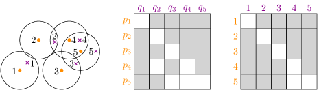
Figure 9: The discrete Fréchet distance: (left) two point sequences $P$ (disks) and $Q$ (crosses) with $5$ points each; (middle) the associated free-space matrix $F$ ($\text{white }=1,\text{gray }=0$); (right) the resulting reachability matrix $M$. Since $M_{55}=1$, the discrete Fréchet distance is at most $1$.

We now describe a subquadratic pointer machine algorithm for the decision version. Thus, let point sequences $P$, $Q$ be given, and suppose without loss of generality that $\delta=1$. The discrete analogue of the free-space diagram is an $n\times n$ Boolean matrix $F$ where $F_{ij}=1$, if $d(p_{i},q_{j})\leq 1$, and $F_{ij}=0$, otherwise, for $i,j=1,\dots,n$. We call $F$ the free-space matrix. Similarly, the discrete analogue of the reachable region is an $n\times n$ Boolean matrix $M$ that is defined recursively as follows: $M_{11}=F_{11}$, and for $i,j=1,\dots,n$, $(i,j)\neq 1$, we have $M_{ij}=1$ if and only if $F_{ij}=1$ and at least one of $M_{i-1,j}$, $M_{i,j-1}$ or $M_{i-1,j-1}$ equals $1$ (we set $M_{i,0}=M_{0,j}=0$, for $i,j=1,\dots n$). Then the discrete Fréchet distance between $P$ and $Q$ is at most $1$ if and only if $M_{nn}=1$. We call $M$ the reachability matrix; see Figure 9.

Adapting the method of Agarwal et al. [1], we show how to use preprocessing and table lookup in order to decide whether $M_{nn}=1$ in $o(n^{2})$ steps on a pointer machine. Let $\tau=\lambda\log n$, for a suitable constant $\lambda>0$. We subdivide the rows of $M$ into $k=O(n/\tau)$ strips, each consisting of $\tau$ consecutive rows: the first strip $L_{1}$ consists of rows $1,\dots,\tau$, the second strip $L_{2}$ consists of rows $\tau+1,\dots,2\tau$, and so on. Each strip $L_{i}$, $i=1,\dots,k$, corresponds to a contiguous subsequence $P_{i}$ of $\tau$ points on $P$. Let $\mathcal{A}_{i}$ be the arrangement of disks obtained by drawing a unit disk around each vertex in $P_{i}$. The arrangement $\mathcal{A}_{i}$ has $O(\tau^{2})$ faces.

Next, let $\rho=\lambda\log n/\log\log n$, with $\lambda>0$ as above. We subdivide each strip $L_{i}$, $i=1,\dots,k$ into $l=O(n/\rho)$ elementary boxes, each consisting of $\rho$ consecutive columns in $L_{i}$. We label the elementary boxes as $B_{ij}$, for $i=1,\dots,k$ and $j=1,\dots,l$. As above, an elementary box $B_{ij}$ has corresponding contiguous subsequences $P_{i}$ of $\tau$ vertices on $P$ and $Q_{j}$ of $\rho$ vertices on $Q$. Now, the incomplete signature of an elementary box $B_{ij}$ consists of (i) the index $i$ of the strip that contains it; and (ii) the sequence $f_{1},f_{2},\dots,f_{\rho}$ of faces in the disk arrangement $\mathcal{A}_{i}$ that contain the $\rho$ vertices of $Q_{j}$, in that order. The full signature of an elementary box $B_{ij}$ consists of its incomplete signature plus a sequence of $\rho+\tau$ bits, that represent the entries in the reach matrix $M$ directly above and to the left of $B_{ij}$. We call these bits the reach bits. As in the continuous case, the information in the full signature suffices to determine how the reachability information propagates through the elementary box; see Figure 10.

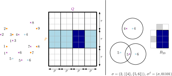
Figure 10: (left) We subdivide the reachability matrix $M$ into strips of $\tau$ rows. Each strip is subdivided into elementary boxes of $\rho$ columns. Each elementary box corresponds to a subsequence of length $\tau$ on $P$ and a subsequence of length $\rho$ on $Q$. (right) The incomplete signature $\sigma$ of an elementary box $B_{ij}$ consists of the index of the containing strip and the face sequence for $Q_{j}$ in $\mathcal{A}_{i}$. The full signature $\sigma^{f}$ additionally contains $\rho+\tau$ reach bits that represent the bits in $M$ directly above and to the left of $B_{ij}$.

The preprocessing phase proceeds as follows: first, we enumerate all possible incomplete signatures. For this, we need to compute all strips $L_{i}$ and the corresponding disk arrangements $\mathcal{A}_{i}$, for $i=1,\dots,\tau$. Furthermore, we also compute a suitable point location structure for each $\mathcal{A}_{i}$. Since there are $O(n/\tau)$ strips, each of which consists of $\tau$ rows, this takes time $O((n/\tau)\cdot\tau^{2}\log\tau)$ = $O(n\tau\log\tau)=O(n\log n\log\log n)$. For each strip $L_{i}$, since $\mathcal{A}_{i}$ has $O(\tau^{2})$ faces, the number of possible face sequences $f_{1},\dots,f_{\rho}$ is $\tau^{O(\rho)}\leq n^{1/3}$, by our choice of $\tau$ and $\rho$ and for $\lambda$ small enough. Thus, there are $O(n^{4/3}/\log n)$ incomplete signatures, and they can be enumerated in the same time. Now, for each incomplete signature $\sigma=(i,\langle f_{1},\dots,f_{\rho}\rangle)$ we build a lookup-table that encodes for each possible setting of the reach bits the resulting reach bits at the bottom and the right boundary of the elementary box. There are $2^{\rho+\tau}\leq n^{1/3}$ possible settings of the reach bits, by our choice of $\tau$ and $\rho$ and for $\lambda$ small enough. We enumerate all of them and organize them as a complete binary tree of depth $\rho+\tau$. For each setting of the reach bits, we use the information of the incomplete signature to determine the result through a straightforward dynamic programming algorithm [39, 1, 19] in $O(\tau\cdot\rho)=O(\log^{2}n)$ time, and we store the result as a linked list of length $\rho+\tau-1$ at the leaf for the corresponding reach bits; see Figure 11. Thus, the total time for this part of the preprocessing phase is $O(n^{5/3}\log n)$.

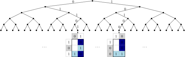
Figure 11: For each incomplete signature, we create a lookup table organized as a complete binary tree. Each leaf corresponds to a setting of the reach bits for the elementary box. In the leaves, we store a linked list of length $\rho+\tau-1$ that represents the contents of the reachability matrix at the bottom and at the right of the elementary box.

Next, we determine for each elementary box $B_{ij}$ its incomplete signature. For this, we use the point location structure for $\mathcal{A}_{i}$ to determine for each vertex in $Q_{j}$ the face of $\mathcal{A}_{i}$ that contains it. There are $O(n^{2}/\tau\rho)$ elementary boxes, each $Q_{j}$ has $\rho$ vertices, and one point location query takes $O(\log\tau)$ time, so the total time for this step is $O((n^{2}/\tau\rho)\cdot\rho\cdot\log\tau)=O((n^{2}/\log n)\log\log n)$. Using this information, we can store with each elementary box a pointer to the lookup table for the corresponding incomplete signature.

Finally, we can now use the lookup tables to propagate the reachability information through $M$, one elementary box at a time, as in the continuous case. The time to process one elementary box is $O(\rho+\tau)$, because we need to traverse the corresponding lookup table to find the reach bits for the adjacent boxes. Thus, the total running time is $O((n^{2}/\tau\rho)\cdot(\rho+\tau))=O(n^{2}/\rho)=O((n^{2}/\log n)\log\log n)$. Thus, we get the following pointer machine version of the result by Agarwal et al. [1]

Theorem 8.1.

There is an algorithm that solves the decision version of the discrete Fréchet problem in $O((n^{2}/\log n)\log\log n)$ time on a pointer machine.

Remark

Agarwal et al. [1] further describe how to get a faster algorithm for the decision version by aggregating the elementary boxes into larger clusters, similar to the method given in Section 6. This improved algorithm finally leads to a subquadratic algorithm for computing the discrete Fréchet distance. Unfortunately, as in Section 6, it seems that this improvement crucially relies on constant time table lookup, so it does not directly translate to the pointer machine.

The reader may also notice that in this section we could choose $\tau,\rho\approx\log n$, whereas in the previous sections we had $\tau\approx\sqrt{\log n}$. This is due to the slightly different definition of signature: in the discrete case, once the subsequence $P_{i}$ is fixed, there are only $\tau^{O(\rho)}$ possible ways how the subsequence $Q_{j}$ might interact with $P_{i}$. In the continuous case, this does not seem to be so clear, and we work with the weaker bound of $\tau^{O(\tau^{2})}$ possible interactions.

9 Decision Trees

Our results also have implications for the decision-tree complexity of the Fréchet problem. Since in that model we account only for comparisons between input elements, the preprocessing comes for free, and hence the size of the elementary boxes can be increased. Before we consider the continuous Fréchet problem, we first note that a similar result can be obtained easily for the discrete Fréchet problem.

Theorem 9.1.

The discrete Fréchet problem has an algebraic computation tree of depth $\widetilde{O}(n^{4/3})$.

Proof.

First, we consider the decision version: we are given two sequences $P=p_{1},\dots,p_{n}$ and $Q=q_{1},\dots,q_{n}$ of $n$ points in the plane, and we would like to decide whether the discrete Fréchet distance between $P$ and $Q$ is at most $1$. Katz and Sharir [53] showed that we can compute a representation of the set of pairs $(p_{i},q_{j})$ with $\|p_{i}-q_{j}\|\leq 1$ in $\widetilde{O}(n^{4/3})$ steps. This information suffices to complete the reachability matrix without further comparisons. As shown by Agarwal et al. [1], one can then solve the optimization problem at the cost of another $O(\log n)$-factor, which is absorbed into the $\widetilde{O}$-notation. ∎

Given our results above, we prove an analogous statement for the continuous Fréchet distance.

Theorem 9.2.

There exists an algebraic decision tree for the Fréchet problem (decision version) of depth $O(n^{2-\varepsilon})$, for a fixed constant $\varepsilon>0$.

Proof.

We reconsider the steps of our algorithm. The only phases that actually involve the input are the second preprocessing phase and the traversal of the elementary boxes. The reason of our choice for $\tau$ was to keep the time for the first preprocessing phase small. This is no longer a problem. By Lemmas 4.2 and 5.1, the remaining cost is bounded by $O(n\tau^{5}+n^{2}(\log\tau)/\tau)$. Choosing $\tau=n^{1/6}$, we get a decision tree of depth $n\cdot n^{5/6}+n^{2-1/6}\log n$. This is $O(n^{2-(1/6)}\log n)=O(n^{2-\varepsilon})$, for any fixed $0<\varepsilon<1/6$. ∎

10 Weak Fréchet distance

The weak Fréchet distance is a variant of the Fréchet distance where we are allowed to walk backwards along the curves [8]. More precisely, let $P$ and $Q$ be two polygonal curves, each with $n$ edges, and let $\Psi^{\prime}$ be the set of all continuous functions $\alpha\colon[0,1]\rightarrow[0,n]$ with $\alpha(0)=0$ and $\alpha(1)=n$. The weak Fréchet distance between $P$ and $Q$ is defined as

$$d_{\text{wF}}(P,Q):=\inf_{\alpha,\beta\in\Psi^{\prime}}\max_{x\in[0,1]}\|P(\alpha(x))-Q(\beta(x))\|.$$

Compared to the regular Fréchet distance, the set $\Psi^{\prime}$ now also contains non-monotone functions. The weak Fréchet distance was also introduced by Alt and Godau [8], who showed how to compute it in $O(n^{2}\log n)$ worst-case time. We will now use our framework to obtain an algorithm that runs in $o(n^{2})$ expected time on a word RAM.

A Decision Algorithm for the Pointer Machine

As usual, we start with the decision version: given two polygonal curves $P$ and $Q$, each with $n$ edges, decide whether $d_{\text{wF}}(P,Q)\leq 1$. This has an easy interpretation in terms of the free-space diagram. Define an undirected graph $G=(V,E)$ with vertex set $V=\{0,1,\dots,n-1\}^{2}$. The vertex $(i,j)\in V$ corresponds to the cell $C(i,j)$, and there is an edge between two vertices $(i,j)$ and $(i^{\prime},j^{\prime})$ if and only if the two cells $C(i,j)$ and $C(i^{\prime},j^{\prime})$ are neighboring (i.e., if $|i-i^{\prime}|+|j-j^{\prime}|=1$) and the door between them is open. Then, $d_{\text{wF}}(P,Q)\leq 1$ if and only if (i) $|P(0)-Q(0)|\leq 1$; (ii) $|P(n)-Q(n)|\leq 1$; and (iii) the vertices $(0,0)$ and $(n-1,n-1)$ are in the same connected component of $G$, see Figure 12.

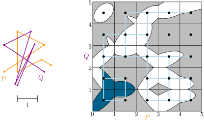
Figure 12: The polygonal curves $P$ and $Q$ have weak Fréchet distance at most $1$, but Fréchet distance larger than $1$: the point $(n,n)$ is not in $\operatorname{reach}(P,Q)$, but the vertices for the cells $C(0,0)$ and $C(4,4)$ are in the same connected component of $G$. The reachable region is shown dark blue, the edges if $G$ are shown light blue.

Let $\tau,\rho\in\mathbb{N}$ be parameters, to be determined later. We subdivide the cells into $k=O(n/\tau)$ vertical strips $L_{1},\dots,L_{k}$, each consisting of $\tau$ consecutive columns. Each strip $L_{i}$ corresponds to a subcurve $P_{i}$ of $P$ with $\tau$ edges. For each such subcurve $P_{i}$, we define two arrangements $\mathcal{A}_{i}$ and $\mathcal{B}_{i}$. To obtain $\mathcal{A}_{i}$, we take for each edge $e$ of $P_{i}$ the “stadium” $c_{e}$ of points with distance exactly $1$ from $e$, and we compute the resulting arrangement. Since two distinct curves $c_{e},c_{e^{\prime}}$ cross in $O(1)$ points, the complexity of $\mathcal{A}_{i}$ is $O(\tau^{2})$, see Figure 13. The arrangement $\mathcal{B}_{i}$ is the arrangement $\mathcal{B}$ described in the proof of Lemma 4.1, i.e., the arrangement of the curves dual to the tangent lines for the unit circles around the vertices of $P_{i}$.

Figure 13: The arrangement $\mathcal{A}_{i}$ for a subcurve $P_{i}$ and the some vertices of $Q$ in it.

Next, we subdivide each strip into $\ell=O(n/\rho)$ elementary boxes, each consisting of $\rho$ consecutive rows. We label the elementary boxes as $B_{ij}$, with $1\leq i\leq k$, $1\leq j\leq\ell$. The rows of an elementary box $B_{ij}$ correspond to a subcurve $Q_{j}$ of $Q$ with $\rho$ edges. The signature of $B_{ij}$ consists of (i) the index $i$ of the corresponding strip; (ii) for each vertex of $Q_{j}$ the face of $\mathcal{A}_{i}$ that contains it; and (ii) for each edge $e$ of $Q_{j}$ the face of $\mathcal{B}_{i}$ that contains the point that is dual to the supporting line of $e$, plus two indices $a,b\in\{1,\dots,\tau\}$ that indicate the first and the last unit circle around a vertex of $P_{i}$ that $e$ intersects, as we walk from one endpoint to another.

Given an elementary box $B$, the connection graph $G_{B}$ of $B$ has $\tau\rho$ vertices, one for each cell in $B$, and an edge between two cells $C$, $C^{\prime}$ of $B$ if and only if $C$ and $C^{\prime}$ share a (horizontal or vertical) edge with an open door. The connectivity list of $B$ is a linked list with $2\tau+2\rho-4$ entries that stores for each cell $C$ on the boundary of $B$ a pointer to a record that represents the connected component of the connection graph $G_{B}$ that contains $C$.

Lemma 10.1.

There are $O(n\tau^{8\rho+1})$ different signatures. The connection graph of an elementary box $B_{ij}$ depends only on its signature, and the connectivity list can be computed in $O(\tau\rho)$ time on a pointer machine, given the signature.

Proof.

First, we count the signatures. There are $O(n/\tau)$ strips. Once the strip index $i$ is fixed, a signature consists of $\rho+1$ faces of $\mathcal{A}_{i}$, $\rho$ faces of $\mathcal{B}_{i}$, and $\rho$ pairs of indices $a,b\in\{1,\dots,\tau\}$. The arrangement $\mathcal{A}_{i}$ has $O(\tau^{2})$ faces, and the arrangement $\mathcal{B}_{i}$ has $O(\tau^{4})$ faces, as explained in the proof of Lemma 4.1. Finally, there are $\tau^{2}$ pairs of indices. Thus, the number of possible signatures in one strip is $\tau^{8\rho+2}$. In total, we get $O(n\tau^{8\rho+1})$ signatures.

Next, the connection graph of an elementary box $B_{ij}$ is determined solely by which doors are open and which doors are closed. We explain how to deduce this information from the signature. A horizontal edge of $B_{ij}$ corresponds to an edge $e$ of $P_{i}$ and a vertex $q$ of $Q_{j}$. The door is open if and only if $q$ has distance at most $1$ from $e$. This is determined by the face of $\mathcal{A}_{i}$ containing $q$. Similarly, a vertical edge of $B_{ij}$ corresponds to a vertex $p$ of $P_{i}$ and an edge $e$ of $Q_{j}$. The door is open if and only if $e$ intersects the unit circle with center $p$. As in Lemma 4.1, this can be inferred from the face of $\mathcal{B}_{i}$ that contains the point dual to the supporting line of $e$, together with the indices $(a,b)$ of the first and last circle intersected by $e$.

Finally, given the signature, we can build the connection graph $G_{B_{ij}}$ in $O(\tau\rho)$ time, assuming that the arrangements $\mathcal{A}_{i}$ and $\mathcal{B}_{i}$ provide suitable data structures. With $G_{B_{ij}}$ at hand, the connection list can be found in $O(\tau\rho)$ steps, using breadth first search. ∎

As usual, our strategy now is to preprocess all possible signatures and to determine the signature of each elementary box. Using this information, we can then process the elementary boxes quickly in our main algorithm. The next lemma describes the preprocessing steps.

Lemma 10.2.

We can determine for each elementary box $B_{ij}$ a pointer to its connectivity list in total time $O(n\tau^{8\rho+2}\rho+(n^{2}/\tau)\log\tau)$ on a pointer machine.

Proof.

First, we compute the arrangements $\mathcal{A}_{i}$ and $\mathcal{B}_{i}$ for each vertical strip. By Lemma 4.1, this takes $O(\tau^{6})$ steps per strip, for a total of $O(\tau^{6}\cdot n/\tau)=O(n\tau^{5})$. Then, we enumerate all possible signatures, and we compute the connectivity list for each of them. By Lemma 10.1, this needs $O(n\tau^{8\rho+2}\rho)$ time. We store the signatures and their connectivity lists

Next, we determine the signature for each elementary box. Fix a strip $L_{i}$. For each vertex $q$ and each edge $e$ of $Q$, we determine the containing faces of $\mathcal{A}_{i}$ and $\mathcal{B}_{i}$ and the pair $(a,b)$ that represents the first and least intersection of $e$ with the unit circles around the vertices of $P_{i}$. This takes $O(n\log\tau)$ steps in total, using appropriate point location structures for the arrangements. Now, we use the data structure from the preprocessing to connect each elementary box to its connectivity list. A simple pointer-based structure supports one lookup in $O(\rho\log\tau)$ time. Since there are $O(n/\rho)$ elementary boxes in one strip, we get a total running time of $O(n\log\tau)$ per strip. Since there are $O(n/\tau)$ strips, the resulting running time is $O((n^{2}/\tau)\log\tau)$. ∎

With the information from the preprocessing phase, we can easily solve the decision problem with a union-find data structure.

Lemma 10.3.

Suppose that each elementary box has a pointer to its connectivity list. Then we can decide whether $d_{wF}(P,Q)\leq 1$ in time $O\big{(}\frac{n^{2}(\tau+\rho)\alpha(n)}{\tau\rho}\big{)}$ on a pointer machine, where $\alpha(\cdot)$ denotes the inverse Ackermann-function.

Proof.

Let $S$ be the set that contains the boundary cells of all elementary boxes. Then, $|S|=O\big{(}\frac{n^{2}(\tau+\rho)}{\tau\rho}\big{)}$. We create a Union-Find data structure for $S$. Then, we go through all elementary boxes $B_{ij}$, and for each $B_{ij}$, we use the connectivity list to connect those subsets of boundary cells that are connected inside $B_{ij}$. This can be done with $O(\tau+\rho)$ Union-operations. Hence, the total running time for this step is $O\big{(}\frac{n^{2}(\tau+\rho)}{\tau\rho}\big{)}$. (We do not need any Find-operations yet, because we can store the representatives of the sets with the representatives of the connected components in the connectivity list as we walk along the boundary of an elementary box.)

Next, we iterate over the boundary cells of all elementary boxes. For each boundary cell $C$, we determine the neighboring boundary cells on neighboring elementary boxes that share an open door with $C$. For each such cell $D$, we perform Find-operations on $C$ and $D$, followed by a Union-operation. This takes $O\big{(}\frac{n^{2}(\tau+\rho)\alpha(n)}{\tau\rho}\big{)}$ time [61]. Finally, we return True if and only if (i) the pairs of start and end vertices of $P$ and $Q$ have distance at most $1$, and (ii) $C(0,0)$ and $C(n-1,n-1)$ are in the same set of the resulting partition of $S$. The running time follows. ∎

The following theorem summarizes our algorithm for the decision problem.

Theorem 10.4.

Let $P$ and $Q$ be two polygonal curves with $n$ edges each. We can decide whether $d_{wF}(p,q)\leq 1$ in $O((n^{2}/\log n)\alpha(n)\log\log n)$ time on a pointer machine, where $\alpha(\cdot)$ denotes the inverse Ackermann function.

Proof.

We set $\tau=\log n$ and $\rho=\lambda\log n/\log\log n$, for a suitable constant $\lambda>0$. If $\lambda$ is small enough, then $\tau^{8\rho+2}=O(n^{4/3})$, and the algorithm from Lemma 10.2 runs in time $O((n^{2}/\log n)\log\log n)$. After the preprocessing is finished, we can use Lemma 10.3 to obtain the final result in time $O((n^{2}/\log n)\alpha(n)\log\log n)$. ∎

A Faster Decision Algorithm on the Word RAM

Theorem 10.4 is too weak to obtain a subquadratic algorithm for the weak Fréchet distance. This requires the full power of the word RAM.

Theorem 10.5.

Let $P$ and $Q$ be two polygonal curves with $n$ edges each. We can decide whether $d_{wF}(p,q)\leq 1$ in $O((n^{2}/\log^{2}n)(\log\log n)^{5})$ time on a word RAM.

Proof.

We set $\tau=\lambda\log^{2}n/\log\log n$ and $\rho=\lambda\log n/\log\log n$. If $\lambda$ is small enough, then $\tau^{8\rho+2}=O(n^{4/3})$, and we can perform the algorithm from Lemma 10.2 in time $O((n^{2}/\log^{2}n)\log\log n)$.

We modify the algorithm from Lemma 10.2 slightly. Instead of a pointer-based connectivity list, we compute a packed connectivity list. It consists of $O(\log n)$ words of $\log n$ bits each. Each word stores $\Theta(\log n/\log\log n)$ entries of $O(\log\log n)$ bits. An entry consists of $O(1)$ fields, each with $O(\log\log n)$ bits. As in Lemma 10.2, the entries in the packed connectivity list represent the connected components of the connection graph $G_{B}$ for the boundary cells of a given elementary box $B$. This is done as follows: each entry of the connectivity list corresponds to a boundary cell $C$ of $B$. In the first field, we store a unique identifier from $\{1,\dots,2\tau+2\rho-4\}$ that identifies $C$. In the second field, we store the smallest identifier of any boundary cell of $B$ that lies in the same connected component as $C$. The remaining fields of the entry are initialized to $0$. Furthermore, we compute for each elementary box $B$ a sequence of $O((\tau/\log n)\log\log n)$ words that indicates for each boundary cell of $B$ whether the corresponding door to the neighboring elementary box is open. This information can be obtained in the same time by adapting the algorithm from Lemma 10.2.

Next, we group the elementary boxes into clusters. A cluster consists of $\log n$ vertically adjacent elementary boxes from a single strip. The first set of clusters come from bottommost $\log n$ elementary boxes, the second set of clusters from following $\log n$ elementary boxes, etc. The boundary and the connectivity list of a cluster are defined analogously as for an elementary box. Below, in Lemma 10.6, we show that we can compute the (pointer-based) connectivity list of a cluster in time $O((\tau+\rho)(\log\log n)^{4})$. Then, the lemma follows: there are $O(n^{2}/(\tau\rho\log n))$ clusters, so the total time to find connectivity lists for all clusters is $O(n^{2}/(\rho\log n)(\log\log n)^{4}+n^{2}/(\tau\log n)(\log\log n)^{4})=O((n^{2}/\log^{2}n)(\log\log n)^{5})$. After that, we can solve the decision problem in time

$$O\left(\frac{n^{2}(\tau+\rho\log n)\alpha(n)}{\tau\rho\log n}\right)=O\left(\frac{n^{2}\alpha(n)\log\log n}{\log^{2}n}\right),$$

as in Lemma 10.3. ∎

Lemma 10.6.

Given a cluster, we can compute the connectivity list for its boundary in total time $O((\tau+\rho)(\log\log n)^{4})$ on a word RAM.

Proof.

Our algorithm makes extensive use of the word RAM capabilities. Data is processed in packed form. That is, we usually deal with a sequence of packed words, each with $O(\log n/\log\log n)$ entries. Each entry has $O(1)$ fields of $O(\log\log n)$ bits. We restrict the number of entries in each word so that the total number of bits used is at most, say, $(1/3)\log n$. Then, we can support any reasonable binary operation on two packed words in $O(1)$ time after $o(n)$ preprocessing time. Indeed, we only need to build a lookup-table during the preprocessing phase. First, we observe that we can sort packed data efficiently.

Claim 10.7.

Suppose we are given a sequence of $\mu$ packed words, representing a sequence of $O(\mu(\log n/\log\log n))$ entries. We can obtain a sequence of $\mu$ packed words that represents the same entries, sorted according to any given field, in $O(\mu\log\mu)$ time.

Proof.

We adapt usual techniques for packed integer sorting [5]. We precompute a merge-operation that receives two packed words, each with their entries sorted according to a given field, and returns two packed words that represent the sorted sequence of all entries. We also precompute an operation that receives one packed word and returns a packed word with the same entries, sorted according to a given field. Then, we can perform a merge sort in $O(\mu\log\mu)$ time, because in each level of the recursion, the total time for merging is $O(\mu)$. Once we are down to a single word, we can sort its entries in one step. More details can be found in the literature on packed sorting [5, 28]. ∎

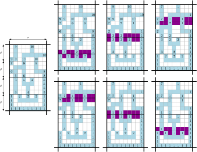
Figure 14: The algorithm for computing the connected components within a cluster. In the beginning, we know the components inside each elementary box (left). In the first phase (top right), we update the connectivity information from bottom to top, by considering the upper and lower boundaries of the vertically adjacent elementary boxes. In the second phase (bottom right), we propagate the connected components from top to bottom.

Now we describe the strategy of the main algorithm. As explained above, a cluster consists of $\log n$ vertically adjacent elementary boxes. We number the boxes $B_{1},\dots,B_{\log n}$, from bottom to top. For $i=1,\dots,\log n$, we denote by $G_{i}$ the connection graph for the boxes $B_{1},\dots,B_{i}$. That is, $G_{i}$ is obtained by taking the union $\bigcup_{j=1}^{i}G_{B_{j}}$ of the individual connection graphs and adding edges for adjacent cells in neighboring boxes that share an open door. Our algorithm proceeds in two phases. In the first phase, we propagate the connectivity information upwards. That is, for $i=1,\dots,\log n$, we compute a sequence $W_{i}$ of $O((\tau+\rho)\log\log n/\log n)$ packed words. Each entry in $W_{i}$ corresponds to a cell $C$ on the boundary of $B_{i}$. The first field stores a unique identifier for the cell, and the second entry stores an identifier of the connected component of $C$ in $G_{i}$. In the second phase, we go in the reverse direction. For $i=\log n,\dots,1$, we compute a sequence $W_{i}^{\prime}$ of $O((\tau+\rho)\log\log n/\log n)$ packed words that store for each cell $C$ on the boundary of $B_{i}$ an identifier of the connected component of $C$ in $G_{\log n}$. Once this information is available, the (pointer-based) connectivity list for the cluster boundary can be extracted in $O(\tau+\rho)$ time, using appropriate precomputed operations on packed words, see Figure 14 .

We begin with the first phase. The upper boundary of an elementary box are the $\tau$ cells in the topmost row of the box, the lower boundary are the $\tau$ cells in the bottommost row. From the preprocessing phase, we have a pointer to the packed connectivity lists for all elementary boxes $B_{1},\dots,B_{\log n}$. We make local copies of these packed connectivity lists, and we modify them so that the identifiers of all cells and connected components are unique. For example, we can increase all identifiers in the connectivity list for $B_{i}$ by $i\log^{3}n$. Using lookup-tables for these word-operations, this step can be carried out in $O((\tau+\rho)\log\log n)$ time for the whole cluster.

The sequence $W_{1}$ for $B_{1}$ is exactly the packed connectivity list of $G_{1}$. Now, suppose that we have computed for $B_{i}$ a sequence $W_{i}$ of packed words that represent the connected component in $G_{i}$ for each boundary cell of $B_{i}$. We need to compute a similar sequence $W_{i+1}$ for $B_{i+1}$. For this, we need to determine how the doors between $B_{i}$ and $B_{i+1}$ affect the connected components in $G_{B_{i+1}}$.

Let $H=(V_{H},E_{H})$ be the graph that has one vertex for each connected component of $G_{i}$ that contains a cell at the upper boundary of $B_{i}$ and one vertex for each connected component of $G_{B_{i+1}}$ that contains a cell at the lower boundary of $B_{i+1}$. The vertices of $H$ are labeled by the identifiers of their corresponding components. Suppose that $v\in V_{H}$ represents a component $D_{v}$ in $G_{i}$ and $w\in V_{H}$ represents a component $D_{w}$ in $G_{B_{i+1}}$. There is an edge between $v$ and $w$ in $E_{H}$ if and only if $D_{v}$ contains a cell on the upper boundary of $B_{i}$ and $D_{w}$ contains a cell on the lower boundary of $B_{i+1}$ such that these two cells share an open door. The graph $H$ has $O(\tau)$ vertices and $O(\tau)$ edges. Our goal is to obtain the connected components of $H$. From this, we will then derive the next sequence $W_{i+1}$. To obtain the components of $H$, we adapt the parallel connectivity algorithm of Hirschberg, Chandra, and Sarwate [50].

Claim 10.8.

We can determine the connected components of $H$ in time $O((\tau/\log n)\log\log^{4})$ time.

Proof.

First, we obtain a list of $O((\tau/\log n)\/\log\log n)$ packed words that represent the vertices of $H$, as follows: we extract from $W_{i}$ and from the connectivity list of $B_{i+1}$ the entries for the upper boundary of $B_{i}$ and for the lower boundary of $B_{i+1}$. If all these entries are stored together in the respective packed lists, this takes $O((\tau/\log n)\log\log n)$ time to copy the relevant data words. Then, we sort these packed sequences according to the component identifier, in time $O(\tau/\log n)\log\log^{2}n)$ (Claim 10.7). Finally, we go over the sorted packed sequence to extract a sorted lists of the distinct component identifiers. This takes $O((\tau/\log n)\log\log n)$ time, using an appropriate operation on packed words.

The edges of $E_{H}$ can also be represented by a sequence of $O((\tau/\log n)\log\log n)$ words. As explained above, we have from the preprocessing phase for each elementary box a sequence of $O((\tau/\log n)\log\log n)$ words whose entries indicate the open doors along its upper boundary. From this, we can obtain in $O((\tau/\log n)\log\log n)$ time a sequence of $O((\tau/\log n))\log\log n)$ words whose entries represent the edges of $H$, where each entry stores the component identifiers of the two endpoints of the edge. We are now ready to implement the algorithm of Hirschberg, Chandra, and Sarwate. The main steps of the algorithm are as follows, see Figure 15.

Figure 15: The algorithm of Hirschberg, Chandra, and Sarwate. In each step, we either connect all nodes to their largest neighbor or to their smallest neighbor. Then, we contract the resulting rooted trees and label the contracted nodes with the index of the smallest node.

Step 1: Find for each vertex of $H$ the neighbor with the smallest and with the largest identifier. This can be done in $O((\tau/\log n)\log\log^{2}n)$ time by sorting the edge lists twice, once in lexicographic order and once in reverse lexicographic order of the identifiers of the endpoints. From these sorted lists, we can extract the desired information in the claimed time, using appropriate word operations.

Step 2: Let $V_{H}^{\prime}$ be the vertices of $H$ with at least one neighbor, and let $V_{H}^{\prime\prime}\subseteq V_{H}^{\prime}$ be the vertices $v\in V_{H}^{\prime}$ having a neighbor with a smaller identifier than the identifier of $v$. If $|V_{H}^{\prime\prime}|\geq|V_{H}^{\prime}|/2$, we set the successor of each $v\in V_{H}^{\prime\prime}$ to the neighbor of $v$ with the smallest identifier. Otherwise, at least half of the nodes in $V_{H}^{\prime}$ have a neighbor with a larger identifier. In this case, we let $V_{H}^{\prime\prime\prime}$ be the set of these nodes, and we set the successor of each $v\in V_{H}^{\prime\prime\prime}$ to the neighbor of $v$ with the largest identifier. The successor relation defines a directed forest $F$ on $V_{H}$ such that at least half of the vertices in $V_{H}^{\prime}$ are not a root in $F$. Given the information available from Step 1 and appropriate word operations, this step can carried out in $O((\tau/\log n)\log\log n)$ time.

Step 3: Use pointer jumping to determine for each vertex $v\in V_{H}$ the identifier of the root of the tree in $F$ that contains $v$. For this, we set the successor of each $v\in V_{H}$ that does not yet have a successor to $v$ itself. Then, for $\log|V_{H}|=O(\log\log n)$ rounds, we set simultaneously for each $v\in V_{H}$ the new successor of $v$ to the old successor of the old successor of $v$ (pointer jumping). Each step at least halves the distance of $v$ to its root in $F$, so it takes $O(\log|V_{H}|)$ rounds until each vertex in $V_{H}$ has found the root of its tree in $F$. Each round can be implemented in $O((\tau/\log n)\log\log^{2}n)$ time by sorting the vertices according to their successors. Thus, this step takes $O((\tau/\log n)\log\log^{3}n)$ time in total.

Step 4: Contract each tree of $F$ into a single vertex whose identifier is the smallest identifier in the tree.. Maintain for the original vertices of $H$ a list that gives the identifier of the contracted node that represents it. Again, this step can be carried out in $O(\tau/\log n)\log\log^{2}n)$ time using sorting.

After Steps 1–4, the number of non-singleton components in $H$ has at least halved. Thus, by repeating the steps $O(\log|V_{H}|)=O(\log\log n)$ times, we can identify the connected components of $H$. The total time of the algorithm is $O((\tau/\log n)\log\log^{4}n)$, as claimed. ∎

Given the connected components of $H$, we can find the desired sequence $W_{i+1}$ for the boundary $B_{i+1}$. Indeed, the procedure from Claim 10.8 outputs a sequence of $O((\tau/\log n)\log\log n)$ packed words that gives for each vertex in $H$ an identifier of the component in $H$ that contains it. We can use this list as a lookup table to update the identifiers of the components in the connectivity list of $B_{i+1}$. This takes $O((\tau+\rho)/\log n)\log\log^{2}n)$ time, using sorting.

In summary, since we consider $\log n$ elementary boxes, the total time for the first phase if $O((\tau+\rho)\log\log^{4}n)$. The second phase is much easier. For $i=\log_{n},\dots,2$, we propagate the connectivity information from $B_{i+1}$ to $B_{i}$. For this, we need to update the identifiers of the connected components for the cells on the upper boundary of $B_{i}$ using the identifiers of the connected components on the lower boundary of $B_{i+1}$, and then adjust the connectivity list $B_{i+1}$ with these new indices. Again, this takes $O((\tau+\rho)/\log n)\log\log^{2}n)$ time, using sorting. ∎

Computing the Weak Fréchet Distance

To actually compute the weak Fréchet distance, we use a simplified version of the procedure from Section 7. In particular, for the weak Fréchet distance, there are only critical values of the type vertex-vertex and vertex-edge, i.e., there are only $O(n^{2})$ critical values. However, we aim for a subquadratic running time, so we need to perform the sampling procedure in a slightly different way.

Theorem 10.9.

Suppose we can answer the decision problem for the weak Fréchet distance in time $T(n)$, for input curves $P$ and $Q$ with $n$ edges each. Then, we can compute the weak Fréchet distance of $P$ and $Q$ in expected time $O(n^{3/2}\log^{c}n+T(n)\log n)$, for some fixed constant $c>0$.

Proof.

First, we sample a set $S$ of $K=6n^{1/2}$ critical values uniformly at random. Then, we find $a,b$ such that the weak Fréchet distance lies between $a$ and $b$ and such that the interval $[a,b]$ contains no other element from $S$. This takes $O(K+T(n)\log n)$ time, using median finding.

Similarly to Har-Peled and Raichel [49, Lemma 6.2], we see that the probability, that the interval $[a,b]$ has more than $2\gamma n^{3/2}\ln n$ critical values is at most $1/n^{\gamma}$. Indeed, there are at most $n^{2}$ vertex-vertex and at most $2n^{2}$ vertex-edge events. Thus, the total number of critical values is at most $L\leq 3n^{2}$. Let $U^{+}$ be the next $\gamma n^{3/2}\ln n$ larger critical values after $d_{\text{wF}}(P,Q)$. Then, the probability that $S$ contains no value from $U^{+}$ is

$$\frac{\binom{L-|U^{+}|}{K}}{\binom{L}{K}}=\prod_{i=0}^{K-1}\left(1-\frac{|U^{+}|}{L-i}\right)\leq\left(1-\frac{|U^{+}|}{L}\right)^{K}\leq\exp\left(-\frac{|U^{+}|K}{L}\right)\leq\exp(-2\gamma\ln n)\leq\frac{1}{2n^{\gamma}}.$$

Analogously, the probability that $S$ contains none of the next $\gamma n^{3/2}\ln n$ smaller critical values is also at most $1/2n^{\gamma}$, so the claim follows. For $\gamma>0$ large enough, the contribution of this event to the expected running time is negligible.

Next, we find all critical values in the interval $[a,b]$. For this, we must determine all vertex-vertex and vertex-edge pairs with distance in $[a,b]$. We report for every vertex $p$ of $P$ or $Q$ the set of vertices of the other curve that lie in the annulus with radii $a$ and $b$ around $p$. Furthermore, we report for every edge $e$ of $P$ or $Q$ the set of vertices of the other curve that lie in the stadium with radii $a$ and $b$. This can be done efficiently with a range-searching structure for semi-algebraic sets. Agarwal, Matoušek and Sharir [3] show that we can preprocess the vertices of $P$ and the vertices of $Q$ into a data structure that can answer our desired range reporting queries in time $O(n^{1/2}\log^{c}n+k)$, where $k$ is the output size and $c>0$ is some fixed constant. The expected preprocessing time is $O(n^{1+\varepsilon})$, where $\varepsilon>0$ can be made arbitrarily small. We perform $O(n)$ queries, and the total expected output size of our queries is $O(n^{3/2}\ln n)$, so it takes expected time $O(n^{3/2}\log^{c}n)$ to find the critical values in $[a,b]$. Finally, we perform a binary search on theses critical values to compute the weak Fréchet distance. This takes $O(T(n)\log n)$ time. ∎

The following theorem summarizes our results on the weak Fréchet distance.

Theorem 10.10.

The weak Fréchet distance of two polygonal curves, each with $n$ edges, can be computed by a randomized algorithm in time $O(n^{2}\alpha(n)\log\log n)$ on a pointer machine and in time $O((n^{2}/\log n)(\log\log n)^{5})$ on a word RAM.

11 Conclusion

We have broken the long-standing quadratic upper bound for the decision version of the Fréchet problem. Moreover, we have shown that this problem has an algebraic decision tree of depth $O(n^{2-\varepsilon})$, for some $\varepsilon>0$ and where $n$ is the number of vertices of the polygonal curves. We have shown how our faster algorithm for the decision version can be used for a faster algorithm to compute the Fréchet distance. If we allow constant-time table-lookup, we obtain a running time in close reach of $O(n^{2})$. This leaves us with intriguing open research questions. Can we devise a quadratic or even a slightly subquadratic algorithm for the optimization version? Can we devise such an algorithm on the word RAM, that is, with constant-time table-lookup? What can be said about approximation algorithms?

Appendix A Computational Models

Real RAM

The standard machine model in computational geometry is the real RAM [56]. Here, data is represented as a (countably) infinite sequence of storage cells. These cells can be of two different types: they can store real numbers or integers. The model supports standard operations on these numbers in constant time, including addition, multiplication, and elementary functions like square-root, sine or cosine. Furthermore, the integers can be used as indices to memory locations. Integers can be converted to real numbers in constant time, but we need to be careful about the reverse direction. The floor function can be used to truncate a real number to an integer, but if we were allowed to use it arbitrarily, the real RAM could solve PSPACE-complete problems in polynomial time [58]. Therefore, we usually have only a restricted floor function at our disposal.

Word RAM

The word RAM is essentially a real RAM without support for real numbers. However, on a real RAM, the integers are usually treated as atomic, whereas the word RAM allows for powerful bit-manipulation tricks [42]. More precisely, the word RAM represents the data as a sequence of $w$-bit words, where $w=\Omega(\log n)$. Data can be accessed arbitrarily, and standard operations, such as Boolean operations (and, xor, shl, $\ldots$), addition, or multiplication take constant time. There are many variants of the word RAM, depending on precisely which instructions are supported in constant time [42, 28]. The general consensus seems to be that any function in $\text{AC}^{0}$ is acceptable. However, it is always preferable to rely on a set of operations as small, and as non-exotic, as possible. Note that multiplication is not in $\text{AC}^{0}$ [43], but nevertheless is often included in the word RAM instruction set [42].

Pointer machine

The pointer machine model disallows the use of constant time table lookup, and is therefore a restriction of the (real) RAM model [59, 61]. The data structure is modeled as a directed graph $G$ with bounded out-degree. Each node in $G$ represents a record, with a bounded number of pointers to other records and a bounded number of (real or integer) data items. The algorithm can access data only by following pointers from the inputs (and a bounded number of global entry records); random access is not possible. The data can be manipulated through the usual real RAM operations, but without support for the floor function, for reasons mentioned above.

Algebraic computation tree

Algebraic computation trees (ACTs) [11] are the computational geometry analogue of binary decision trees, and like these they are mainly used for proving lower bounds. Let $x_{1},\ldots,x_{n}\in{\mathbb{R}}$ be the inputs. An ACT is a binary tree with two kinds of nodes: computation and branch nodes. A computation node $v$ has one child and is labeled with an expression of the type $y_{v}=y_{u}\oplus y_{w}$, where $\oplus\in\{+,-,*,/,\sqrt{\cdot}\}$ is a operator and $y_{u},y_{w}$ is either an input variable $x_{1},\ldots,x_{n}$ or corresponds to a computation node that is an ancestor of $v$. A branch node has degree 2 and is labeled by $y_{u}=0$ or $y_{u}>0$, where again $y_{u}$ is either an input or a variable for an ancestor. A family of algebraic computation trees $(T_{n})_{n\in\mathbb{N}}$ solves a computational problem (like Delaunay triangulation or convex hull computation), if for each $n\in\mathbb{N}$, the tree $T_{n}$ accepts inputs of size $n$, and if for any such input $x_{1},\ldots,x_{n}$ the corresponding path in $T_{n}$ (where the children of the branch nodes are determined according the conditions they represent) constitutes a computation that represents the answer in the variables $y_{v}$ encountered during the path.

Algebraic decision trees are defined as follows: we allow only branch nodes. Each branch node is labeled with a predicate of the form $p(x_{1},\dots,x_{n})=0$ or $p(x_{1},\dots,x_{n})>0$. The leaves are labeled yes or no. Fix some $r\in\{1,\dots,n\}$. If $p$ is restricted to be of the form $p(x_{1},\dots,x_{n})=\sum_{i=1}^{n}a_{i}x_{i}-b$, with at most $r$ coefficients $a_{i}\neq 0$, we call the decision tree $r$-linear. Erickson [40] showed that any $3$-linear decision tree for 3SUM has depth $\Omega(n^{2})$. However, Grønlund and Pettie showed that there is a $4$-linear decision tree of depth $O(n^{3/2}\sqrt{\log n})$ for the problem. In geometric problems, linear predicates are often much too restrictive. For example, there is no $r$-linear decision tree for the Fréchet problem, no matter the choice of $r$: with $r$-linear decision trees, we cannot even decide whether two given points $p$ and $q$ have Euclidean distance at most $1$.

References

- [1] P. K. Agarwal, R. Ben Avraham, H. Kaplan, and M. Sharir. Computing the discrete Fréchet distance in subquadratic time. SIAM J. Comput., 43(2):429–449, 2014.
- [2] P. K. Agarwal, S. Har-Peled, N. H. Mustafa, and Y. Wang. Near-linear time approximation algorithms for curve simplification. Algorithmica, 42(3–4):203–219, 2005.
- [3] P. K. Agarwal, J. Matoušek, and M. Sharir. On range searching with semialgebraic sets. II. SIAM J. Comput., 42(6):2039–2062, 2013.
- [4] N. Ailon and B. Chazelle. Lower bounds for linear degeneracy testing. J. ACM, 52(2):157–171, 2005.
- [5] S. Albers and T. Hagerup. Improved parallel integer sorting without concurrent writing. Inform. and Comput., 136(1):25–51, 1997.
- [6] H. Alt. The computational geometry of comparing shapes. In Efficient Algorithms, volume 5760 of Lecture Notes in Computer Science, pages 235–248. Springer-Verlag, 2009.
- [7] H. Alt and M. Buchin. Can we compute the similarity between surfaces? Discrete Comput. Geom., 43(1):78–99, 2010.
- [8] H. Alt and M. Godau. Computing the Fréchet distance between two polygonal curves. Internat. J. Comput. Geom. Appl., 5(1–2):78–99, 1995.
- [9] H. Alt, C. Knauer, and C. Wenk. Comparison of distance measures for planar curves. Algorithmica, 38(1):45–58, 2003.
- [10] B. Aronov, S. Har-Peled, C. Knauer, Y. Wang, and C. Wenk. Fréchet Distances for Curves, Revisited. In Proc. 14th Annu. European Sympos. Algorithms (ESA), volume 4168 of Lecture Notes in Computer Science, pages 52–63, 2006.
- [11] S. Arora and B. Barak. Computational complexity. A modern approach. Cambridge University Press, Cambridge, 2009.
- [12] I. Baran, E. D. Demaine, and M. Pǎtraşcu. Subquadratic algorithms for 3SUM. Algorithmica, 50(4):584–596, April 2008.
- [13] R. Bellman and R. Kalaba. On adaptive control processes. IRE Transactions on Automatic Control, 4(2):1–9, 1959.
- [14] R. Ben Avraham, O. Filtser, H. Kaplan, M. J. Katz, and M. Sharir. The discrete and semicontinuous Fréchet distance with shortcuts via approximate distance counting and selection. ACM Transactions on Algorithms, 11(4):29:1–29:29, 2015.
- [15] M. de Berg, A. F. Cook IV, and J. Gudmundsson. Fast Fréchet queries. Comput. Geom. Theory Appl., 46(6):747–755, 2013.
- [16] S. Brakatsoulas, D. Pfoser, R. Salas, and C. Wenk. On map-matching vehicle tracking data. In Proc. 31st Int. Conf. on Very Large Data Bases, pages 853–864, 2005.
- [17] D. Bremner, T. M. Chan, E. D. Demaine, J. Erickson, F. Hurtado, J. Iacono, S. Langerman, M. Pǎtraşcu, and P. Taslakian. Necklaces, convolutions, and . Algorithmica, pages 1–21, 2012.
- [18] K. Bringmann. Why walking the dog takes time: Fréchet distance has no strongly subquadratic algorithms unless SETH fails. In Proc. 55th Annu. IEEE Sympos. Found. Comput. Sci. (FOCS), pages 661–670, 2014.
- [19] K. Bringmann and W. Mulzer. Approximability of the discrete Fréchet distance. Journal of Computational Geometry, 7(2):46–76, 2016.
- [20] K. Buchin, M. Buchin, and J. Gudmundsson. Constrained free space diagrams: a tool for trajectory analysis. Int. J. of GIS, 24(7):1101–1125, 2010.
- [21] K. Buchin, M. Buchin, J. Gudmundsson, M. Löffler, and J. Luo. Detecting commuting patterns by clustering subtrajectories. Internat. J. Comput. Geom. Appl., 21(3):253–282, 2011.
- [22] K. Buchin, M. Buchin, C. Knauer, G. Rote, and C. Wenk. How difficult is it to walk the dog? In Proc. 23rd European Workshop Comput. Geom. (EWCG), pages 170–173, 2007.
- [23] K. Buchin, M. Buchin, W. Meulemans, and B. Speckmann. Locally correct Fréchet matchings. In Proc. 20th Annu. European Sympos. Algorithms (ESA), volume 7501 of Lecture Notes in Computer Science, pages 229–240, 2012.
- [24] K. Buchin, M. Buchin, and A. Schulz. Fréchet distance of surfaces: Some simple hard cases. In Proc. 18th Annu. European Sympos. Algorithms (ESA), volume 6347 of Lecture Notes in Computer Science, pages 63–74, 2010.
- [25] K. Buchin, M. Buchin, R. van Leusden, W. Meulemans, and W. Mulzer. Computing the Fréchet distance with a retractable leash. Discrete Comput. Geom., 56(2):315–336, 2016.
- [26] K. Buchin, M. Buchin, and Y. Wang. Exact algorithms for partial curve matching via the Fréchet distance. In Proc. 20th Annu. ACM-SIAM Sympos. Discrete Algorithms (SODA), pages 645–654, 2009.
- [27] K. Buchin, M. Buchin, and C. Wenk. Computing the Fréchet distance between simple polygons. Comput. Geom. Theory Appl., 41(1–2):2–20, 2008.
- [28] K. Buchin and W. Mulzer. Delaunay triangulations in time and more. J. ACM, 58(2):Art. 6, 27, 2011.
- [29] M. Buchin. On the Computability of the Fréchet Distance Between Triangulated Surfaces. PhD thesis, Free University Berlin, Institute of Computer Science, 2007.
- [30] E. Chambers, É. de Verdière, J. Erickson, S. Lazard, F. Lazarus, and S. Thite. Homotopic Fréchet distance between curves or, walking your dog in the woods in polynomial time. Comput. Geom. Theory Appl., 43(3):295–311, 2010.
- [31] T. M. Chan. All-pairs shortest paths with real weights in time. Algorithmica, 50(2):236–243, 2008.
- [32] T. M. Chan. More algorithms for all-pairs shortest paths in weighted graphs. SIAM J. Comput., 39(5):2075–2089, 2010.
- [33] B. M. Chazelle and D. T. Lee. On a circle placement problem. Computing, 36(1–2):1–16, 1986.
- [34] A. F. Cook, A. Driemel, S. Har-Peled, J. Sherette, and C. Wenk. Computing the Fréchet distance between folded polygons. In Proc. 12th Symposium on Algorithms and Data Structures (WADS), pages 267–278, 2011.
- [35] A. F. Cook and C. Wenk. Geodesic Fréchet distance inside a simple polygon. ACM Transactions on Algorithms, 7(1):Art. 9, 2010.
- [36] A. Driemel and S. Har-Peled. Jaywalking your dog: Computing the Fréchet distance with shortcuts. SIAM J. Comput., 42(5):1830–1866, 2013.
- [37] A. Driemel, S. Har-Peled, and C. Wenk. Approximating the Fréchet distance for realistic curves in near linear time. Discrete Comput. Geom., 48(1):94–127, 2012.
- [38] A. Efrat, L. Guibas, S. Har-Peled, J. Mitchell, and T. Murali. New similarity measures between polylines with applications to morphing and polygon sweeping. Discrete Comput. Geom., 28(4):535–569, 2002.
- [39] T. Eiter and H. Mannila. Computing Discrete Fréchet Distance. Technical Report CD-TR 94/65, Christian Doppler Laboratory, 1994.
- [40] J. Erickson. Bounds for linear satisfiability problems. Chicago J. Theor. Comput. Sci., page Article 8, 1999.
- [41] M. L. Fredman. How good is the information theory bound in sorting? Theoret. Comput. Sci., 1(4):355–361, 1975/76.
- [42] M. L. Fredman and D. E. Willard. Surpassing the information theoretic bound with fusion trees. J. Comput. System Sci., 47(3):424–436, 1993.
- [43] M. L. Furst, J. B. Saxe, and M. Sipser. Parity, circuits, and the polynomial-time hierarchy. Mathematical Systems Theory, 17(1):13–27, 1984.
- [44] A. Gajentaan and M. H. Overmars. On a class of problems in computational geometry. Comput. Geom. Theory Appl., 5(3):165–185, 1995.
- [45] M. Godau. A natural metric for curves - computing the distance for polygonal chains and approximation algorithms. In Proc. 8th Sympos. Theoret. Aspects Comput. Sci. (STACS), pages 127–136, 1991.
- [46] M. Godau. On the Complexity of Measuring the Similarity Between Geometric Objects in Higher Dimensions. PhD thesis, Freie Universität Berlin, Germany, 1998.
- [47] J. Gudmundsson and T. Wolle. Towards automated football analysis: Algorithms and data structures. In Proc. 10th Australasian Conf. on Mathematics and Computers in Sport, 2010.
- [48] S. Har-Peled, A. Nayyeri, M. Salavatipour, and A. Sidiropoulos. How to walk your dog in the mountains with no magic leash. In Proc. 28th Annu. ACM Sympos. Comput. Geom. (SoCG), pages 121–130, 2012.
- [49] S. Har-Peled and B. Raichel. The Fréchet distance revisited and extended. ACM Transactions on Algorithms, 10(1):3, 2014.
- [50] D. S. Hirschberg, A. K. Chandra, and D. V. Sarwate. Computing connected components on parallel computers. Commun. ACM, 22(8):461–464, 1979.
- [51] P. Indyk. Approximate nearest neighbor algorithms for Frechet distance via product metrics. In Proc. 18th Annu. ACM Sympos. Comput. Geom. (SoCG), pages 102–106, 2002.
- [52] A. G. Jørgensen and S. Pettie. Threesomes, degenerates, and love triangles. In Proc. 55th Annu. IEEE Sympos. Found. Comput. Sci. (FOCS), pages 621–630, 2014.
- [53] M. Katz and M. Sharir. An expander-based approach to geometric optimization. SIAM J. Comput., 26(5):1384–1408, 1997.
- [54] A. Maheshwari, J.-R. Sack, K. Shahbaz, and H. Zarrabi-Zadeh. Fréchet distance with speed limits. Comput. Geom. Theory Appl., 44(2):110–120, 2011.
- [55] A. Maheshwari, J.-R. Sack, K. Shahbaz, and H. Zarrabi-Zadeh. Improved algorithms for partial curve matching. In Proc. 19th Annu. European Sympos. Algorithms (ESA), volume 6942 of Lecture Notes in Computer Science, pages 518–529, 2011.
- [56] F. P. Preparata and M. I. Shamos. Computational geometry. An introduction. Springer-Verlag, 1985.
- [57] M. Pǎtraşcu. Towards polynomial lower bounds for dynamic problems. In Proc. 42nd Annu. ACM Sympos. Theory Comput. (STOC), pages 603–610, 2010.
- [58] A. Schönhage. On the power of random access machines. In Proc. 6th Internat. Colloq. Automata Lang. Program. (ICALP), pages 520–529, 1979.
- [59] A. Schönhage. Storage modification machines. SIAM J. Comput., 9(3):490–508, 1980.
- [60] M. Sharir and P. K. Agarwal. Davenport-Schinzel Sequences and Their Geometric Applications. Cambridge University Press, 1995.
- [61] R. E. Tarjan. Efficiency of a good but not linear set union algorithm. J. ACM, 22(2):215–225, 1975.
- [62] M. Thorup. Randomized sorting in time and linear space using addition, shift, and bit-wise boolean operations. J. Algorithms, 42(2):205–230, 2002.
- [63] C. Wenk, R. Salas, and D. Pfoser. Addressing the need for map-matching speed: Localizing global curve-matching algorithms. In Proc. 18th Int. Conf. on Sci. and Stat. Database Management, pages 379–388, 2006.