Three dimensional Symmetry Protected Topological Phase close to
Antiferromagnetic Néel order

Abstract

It is well-known that the Haldane phase of one-dimensional spin-1 chain is a symmetry protected topological (SPT) phase, which is described by a nonlinear Sigma model (NLSM) with a $\Theta-$term at $\Theta=2\pi$. In this work we study a three dimensional SPT phase of SU(2$N$) antiferromagnetic spin system with a self-conjugate representation on every site. The spin ordered Néel phase of this system has a ground state manifold $\mathcal{M}=\frac{\mathrm{U}(2N)}{\mathrm{U}(N)\times\mathrm{U}(N)}$, and this system is described by a NLSM defined with manifold $\mathcal{M}$. Since the homotopy group $\pi_{4}[\mathcal{M}]=\mathbb{Z}$ for $N>1$, this NLSM can naturally have a $\Theta-$term. We will argue that when $\Theta=2\pi$ this NLSM describes a SPT phase. This SPT phase is protected by the SU(2$N$) spin symmetry, or its subgroup SU($N$)$\times$SU$(N)\rtimes Z_{2}$, without assuming any other discrete symmetry. We will also construct a trial SU(2$N$) spin state on a 3d lattice, we argue that the long wavelength physics of this state is precisely described by the aforementioned NLSM with $\Theta=2\pi$.

I 1. Introduction

According to the classic Ginzburg-Landau paradigm, all the disordered phases of classical systems are basically equivalent and completely featureless. However, it is now a consensus that quantum disordered phases driven by quantum fluctuation can have much richer structures. Roughly speaking, in quantum many-body systems, quantum mechanics can lead to at least three types of exotic/nontrivial quantum disordered phases: (1) Topological phases with a gapped spectrum and bulk topological degeneracy, (2) algebraic liquid phases with gapless bulk spectrum and power-law correlations, and (3) symmetry protected topological phases. A symmetry protected topological (SPT) phase is a state of matter with gapped and nondegenerate bulk spectrum, but cannot continuously evolve into a direct product state without a bulk phase transition, when and only when the Hamiltonian of the entire evolution is invariant under certain global symmetry $G$ Chen et al. (2011). In terms of its phenomena, a SPT phase on a $d-$dimensional lattice should satisfy at least the following three criteria:

($1$). On a $d-$dimensional lattice without boundary, this phase is fully gapped, and nondegenerate;

($2$). On a $d-$dimensional lattice with a $(d-1)-$dimensional boundary, if the Hamiltonian of the entire system (including both bulk and boundary Hamiltonian) preserves certain symmetry $G$, this phase is either gapless, or gapped but degenerate.

(3). The boundary state of this $d-$dim system cannot be realized as a $(d-1)$-dim lattice system built with the same onsite Hilbert space, and with the same symmetry $G$.

If a $d-$dim quantum disordered phase satisfies all three criteria (1), (2) and (3), this phase is a SPT phase. Both the $2d$ quantum spin Hall (QSH) insulator Kane and Mele (2005a, b); Bernevig et al. (2006) and $3d$ Topological band insulator (TBI) Fu et al. (2007); Moore and Balents (2007); Roy (2009) are perfect examples of SPT phases protected by time-reversal symmetry and charge conservation.

Notice that the second criterion ($2$) implies the following two possibilities: On a lattice with a boundary, the system is either ($2a$) gapless, or ($2b$) gapped but degenerate. When $d\geq 3$, the degeneracy of ($2b$) can correspond to either spontaneous breaking of $G$, or correspond to certain topological degeneracy at the boundary. Which case occurs in the system will depend on the detailed Hamiltonian at the boundary of the system. For example, with interaction, the edge states of 2$d$ QSH insulator, and 3$d$ TBI can both be gapped out through spontaneous time-reversal symmetry breaking at the boundary, and this spontaneous time-reversal symmetry breaking can occur through a boundary transition, without destroying the bulk state Xu and Moore (2006); Wu et al. (2006); Xu (2010a).

In this work we will focus on $bosonic$ spin systems. The simplest example of SPT phase of spin system is the Haldane phase of one dimensional spin-1 chain. In our paper we will first give a review of Haldane phase, focusing on its nonlinear sigma model field theory description in section II. Unlike the free fermion case, although there is a classification of bosonic SPT using group cohomology Chen et al. (2011), specific models of higher dimensional bosonic spin systems are not well understood. So far, in most studies, construction of 2d and 3d bosonic SPTs has been focused on systems with U(1) symmetry Lu and Vishwanath (2012); Levin and Senthil (2012); Vishwanath and Senthil (arXiv:1209.3058). In this work we will study a $3+1$ dimensional analogue of the Haldane phase, which is constructed as a SU(2$N$) spin state with a self-conjugate representation on each site. Just like the Haldane phase, this 3+1d SPT is described by a nonlinear sigma model defined with a semiclassical antiferromagnetic order parameter plus a topological $\Theta-$term.

II 2. Haldane phase

Although symmetry protected topological phase is a pure quantum phenomenon without any classical analogue, the Haldane phase of spin-1 chain can still be described semiclassically by a nonlinear Sigma model (NLSM), which is defined $only$ in terms of the semiclassical Néel order parameter $\vec{n}$ Haldane (1983a, b):

$$\mathcal{L}=\frac{1}{g}(\partial_{\mu}\vec{n})^{2}+\frac{i\Theta}{8\pi}\epsilon_{abc}\epsilon_{\mu\nu}n^{a}\partial_{\mu}n^{b}\partial_{\nu}n^{c}.$$ (1)

When the system has SO(3) symmetry, the entire manifold of the configurations of Néel order parameter is $S^{2}$. If we assume the trivial vacuum has $\Theta=0$, then when $\Theta=2\pi$, this model describes the Haldane phase.

Haldane phase is a 1d SPT phase protected by SO(3) spin rotation symmetry, namely as long as the SO(3) symmetry is preserved, no other symmetry (such as time-reversal symmetry, reflection, etc.) is required to protect the Haldane phase . This conclusion was established through previous numerical simulations Pollmann et al. (2012). The field theory Eq. 1 gives us the same conclusion, if it is handled correctly.

The physical meaning of the $\Theta-$term in a NLSM is usually interpreted as a factor $\exp(i\Theta)$ attached to every instanton event in the space-time. Then this interpretation would lead to the conclusion that $\Theta=2\pi$ is equivalent to $\Theta=0$. However, this interpretation is very much incomplete, because it only tells us that theories with $\Theta=2\pi$ and $0$ have the same partition function when the system is defined on a compact manifold. However, once we take an open boundary condition in either space or time, the difference between $\Theta=2\pi$ and $0$ will be explicitly exposed. For example, at the spatial boundary of the $1d$ system, $i.e.$ the interface between $\Theta=0$ and $2\pi$, the $\Theta-$term reduces to a 0+1$d$ O(3) Wess-Zumino-Witten (WZW) term at level 1, whose ground state has two fold degeneracy, thus the boundary is effectively a free spin-1/2 degree of freedom Ng (1994), which is exactly the physics of Haldane phase. If we keep an open boundary at temporal direction, then one can explicitly derive the ground state wave function of Eq. 1 at strong coupling, and we can also see that the ground state of $\Theta=2\pi$ and $\Theta=0$ are very different Xu and Senthil (2013).

We can also define time-reversal transformation: $Z_{2}^{T}:t\rightarrow-t$, $\vec{n}\rightarrow-\vec{n}$, $i\rightarrow-i$, Eq. 1 is always invariant under $Z_{2}^{T}$ (notice that $\tau=it$ is invariant under $Z_{2}^{T}$), no matter which value $\Theta$ takes. In fact, using the renormalization group calculation( Levine et al. (1983, 1984a, 1984b, 1984c), for a more recent review, see Ref. Pruisken et al., 2001), and the general nonperturbative argument in Ref. Xu and Ludwig, 2011, we can derive a phase diagram for model Eq. 1: The system is topological when $\Theta\in\left((4k+1)\pi,(4k+3)\pi\right)$, while the system is trivial when $\Theta\in\left((4k-1)\pi,(4k+1)\pi\right)$; $\Theta=(2k+1)\pi$ is the transition, where the bulk of the system is either gapless, or two fold degenerate. Thus $\Theta=0$ and $2\pi$ are two different stable fixed points.

This phase diagram can be understood as follows: The bulk partition function of Eq. 1 is obviously symmetric around $\Theta=2\pi$ ($\Theta=2\pi\pm\epsilon$ have the same partition function), thus $\Theta=2\pi$ is a fixed point that does not flow under RG. Tuning $\Theta$ slightly away from $2\pi$ will not close the bulk gap, so it can only affect the edge state. However, given that the boundary is a dangling spin-1/2, then no perturbation can be added to the Hamiltonian that can lift the spin-1/2 degeneracy at the boundary, as long as the system has SO(3) symmetry, regardless of other discrete symmetries. Thus if $\Theta$ is tuned slightly away from $2\pi$, namely $\Theta=2\pi\pm\epsilon$, as long as the system still has SO(3) symmetry, the edge spin-1/2 doublet is still stable Ng (1994); Xu and Ludwig (2011). Thus $\Theta=2\pi\pm\epsilon$ is in the same phase as $\Theta=2\pi$. A similar effect was also discussed in the context of 1+1d QED Coleman (1976). The edge state can only be destroyed through a bulk transition, which occurs at the transition $\Theta=\pi$. In this sense $\Theta=2\pi$ is a stable fixed point of an entire Haldane phase. Thus the Haldane phase is a SPT phase that requires SO(3) spin rotation symmetry only.

Now let us couple two Haldane phases to each other:

$$\mathcal{L} = \frac{1}{g}(\partial_{\mu}\vec{n}_{1})^{2}+\frac{i2\pi}{8\pi}\epsilon_{abc}\epsilon_{\mu\nu}n^{a}_{1}\partial_{\mu}n^{b}_{1}\partial_{\nu}n^{c}_{1}$$ (2)

$$+ 1\rightarrow 2+A(\vec{n}_{1}\cdot\vec{n}_{2}).$$ (4)

When $A=-\infty$, effectively $\vec{n}_{1}=\vec{n}_{2}=\vec{n}$, then the system is effectively described by one O(3) NLSM with $\Theta=4\pi$; while when $A=+\infty$, the effective NLSM for the system has $\Theta=0$. When parameter $A$ is tuned from $-\infty$ to $+\infty$, the entire phase diagram with $A\in(-\infty,+\infty)$ is gapped in the bulk. Thus the theory with $\Theta=4\pi$ and $\Theta=0$ are equivalent. This analysis implies that with SO(3) symmetry, $1d$ spin systems have two different classes: there is a trivial class with $\Theta=4\pi k$, and a nontrivial Haldane class with $\Theta=(4k+2)\pi$. This $Z_{2}$ classification is consistent with the group cohomology formalism developed in Ref. Chen et al. (2011).

There are various ways of describing the Haldane phase on a lattice. In the follows we will choose one particular description that will be generalized to higher dimensions later. The Haldane phase can be described on a lattice as follows: On every site we introduce a slave fermion with both spin-1/2 index and SU(2) color index: $f_{i,A,\alpha}$, and the spin-1 operator is represented as Xu et al. (2012)

$$\vec{S}_{j}=\frac{1}{2}\sum_{A=1}^{2}f^{\dagger}_{j,A,\alpha}\vec{\sigma}_{\alpha\beta}f_{j,A,\beta}.$$ (5)

In order to match the slave fermion Hilbert space with the spin-1 Hilbert space, we have to impose two different constraints on each site:

$$\sum_{\alpha,A}f^{\dagger}_{i,A,\alpha}f_{i,A,\alpha}=2,\ \ \ \sum_{\alpha,A,B}f^{\dagger}_{j,A,\alpha}\rho^{\mu}_{AB}f_{j,B,\alpha}=0,$$ (6)

where $\rho^{\mu}$ are three Pauli matrices of the color space. The second constraint guarantees that on every site the color space is in a total antisymmetric representation, thus the spin is in a total symmetric spin-1 representation.

The Haldane phase corresponds to the following mean field state of $f_{A,\alpha}$: $f_{1,\alpha}$ forms valence bonds on links $(2i,2i+1)$, while $f_{2,\alpha}$ forms valence bonds on links $(2i+1,2i+2)$ (Fig. 1$a$). In terms of low energy field theory of the slave fermion, the Haldane phase is described by the following Lagrangian:

$$\mathcal{L}=\bar{\psi}\gamma_{\mu}\partial_{\mu}\psi+m_{0}\bar{\psi}\rho^{z}\psi.$$ (7)

Here the Dirac fermion $\psi$ is the low energy mode of $f$, which is expanded at the two Fermi points $k_{f}=\pm\pi/2$ in the 1d Brillouin zone. If we couple the Néel order parameter to the slave fermion,

$$(-1)^{j}\vec{n}_{j}\cdot\sum_{A}f^{\dagger}_{j,A,\alpha}\vec{\sigma}_{\alpha\beta}f_{j,A,\beta}\sim\vec{n}\cdot\bar{\psi}\gamma_{5}\vec{\sigma}\psi,$$ (8)

Eq. 1 can be derived after integrating out the slave fermions Abanov and Wiegmann (2000), and the derived $\Theta$ is precisely $2\pi$. Notice that in Eq. 7 the gauge fields introduced by constraints Eq. 6 are ignored, but in 1+1 dimension gauge fields are always confining, once the matter fields are gapped.

The Haldane phase is a SPT phase only when the color-singlet constraint $f^{\dagger}_{j}\rho^{\mu}f_{j}=0$ is strictly imposed on every site, $i.e.$ when the Hilbert space on every site is rigorously spin-1. If this constraint is given up, the Hilbert space on every site is enlarged to 6 dimension, and the Haldane phase becomes trivial, because it can now be adiabatically connected to a direct product state with spin-singlet on every site. Actually, besides the Haldane phase mass gap $m_{0}$, we can consider another mass gap $m_{1}\bar{\psi}\gamma_{5}\rho^{z}\psi$ of the Dirac fermion $\psi$. Physically $m_{1}$ corresponds to a “color density wave” on the lattice, which is not allowed if the color singlet constraint is imposed strictly on every site. Without the color singlet constraint, the Haldane phase can adiabatically evolve into the color density wave state, by turning on $m_{1}$.

In this section we have reviewed the physics of Haldane phase. For Haldane phase we have both field theory description, and lattice spin wave function. Most importantly, the field theory with topological term can be precisely derived from the lattice wave function. In the next section, we will achieve the same level of understanding for a 3d generalization of Haldane phase.

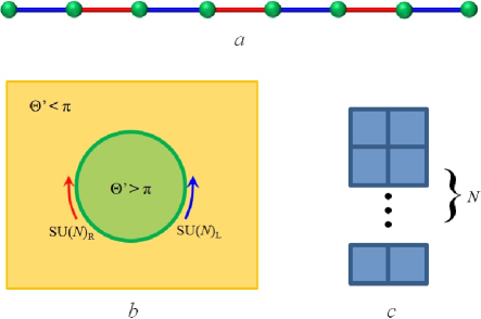
Figure 1: ($a$). The pictorial representation of the Haldane phase, where the blue and red links stand for the valence bonds of slave fermions with color $A=1$ and $2$ respectively. ($b$) A domain wall of $\Theta^{\prime}$ on the boundary of our 3$d$ SPT. ($c$) The Young diagram of the self-conjugate representation of the SU(2$N$) spin system that we are considering.

III 3. 3d SPT phase of SU(2$N$) spin system

III.1 3.1 Field Theory Description

Let us try to look for higher dimensional generalizations of the Haldane phase of spin-1 chain, which has a description in terms of NLSM plus a $\Theta-$term. The most naive generalization would be the AKLT state in higher dimensions, for instance the spin-2 AKLT phase on the square lattice. The boundary of the spin-2 AKLT phase on the square lattice is a spin-1/2 chain, which according to the LSM theorem cannot be gapped and nondegenrate, thus the spin-2 AKLT state seems to be a SPT phase. However, in order to protect the spin-2 AKLT state, we need translation symmetry, since the boundary spin-1/2 chain can be dimerized and gapped out once the translation symmetry of the system is explicitly broken. Thus this is not an ideal generalization of the $1d$ Haldane phase, whose stability does not rely on any translation symmetry. The spin-2 AKLT state on the square lattice can indeed be described by a NLSM with a topological term, but the configurational space of this NLSM would involve both the Néel and dimerization order parameters.

The goal of this paper is to find a three dimensional SPT phase without assuming the translation symmetry. Inspired by Eq. 1, we should first look for magnetic systems, whose ground state manifold $\mathcal{M}$ of the spin ordered phase has a nontrivial homotopy group $\pi_{4}[\mathcal{M}]=\mathbb{Z}$, then this SPT can be described by a NLSM defined in manifold $\mathcal{M}$ with a $\Theta-$term. The SU(2$N$) antiferromagnet with self-conjugate representation satisfies this criterion: its magnetic ordered phase has GSM Read and Sachdev (1990, 1989)

$$\mathcal{M}=\frac{\mathrm{U}(2N)}{\mathrm{U}(N)\times\mathrm{U}(N)},\ \ \ \pi_{4}[\mathcal{M}]=\mathbb{Z},\ \mathrm{for}\ N\geq 2.$$ (9)

Every Néel order configuration $\mathcal{P}\in\mathcal{M}$ can be represented as

$$\mathcal{P}=V^{\dagger}\Omega V,\ \ \ \Omega=\left(\begin{array}[]{cccc}\mathbf{1}_{N\times N},&\mathbf{0}_{N\times N}\\ \\ \mathbf{0}_{N\times N},&\mathbf{-1}_{N\times N}\end{array}\right)$$ (13)

where $V$ is a SU(2$N$) matrix. $\mathcal{P}$ is a hermitian traceless order parameter that satisfies $\mathcal{P}^{2}=\mathbf{1}$. In fact, when $N=1$, $\mathcal{M}$ is precisely $S^{2}$, and $\mathcal{P}$ can always be represented as $\mathcal{P}=\vec{n}\cdot\vec{\sigma}$, where $\vec{n}$ is the Néel vector.

Since $\pi_{4}[\mathcal{M}]=\mathbb{Z}$, the following NLSM defined on $\mathcal{M}$ can be written down:

$$\mathcal{S} = \int d^{3}xd\tau\ \frac{1}{g}\mathrm{tr}[\partial_{\mu}\mathcal{P}\partial_{\mu}\mathcal{P}]$$ (14)

$$+ \frac{i\Theta}{256\pi^{2}}\mathrm{tr}[\mathcal{P}\partial_{\mu}\mathcal{P}\partial_{\nu}\mathcal{P}\partial_{\rho}\mathcal{P}\partial_{\lambda}\mathcal{P}]\epsilon_{\mu\nu\rho\lambda}.$$ (16)

By tuning the parameter $g$, there is obviously an order-disorder transition. When $g$ is small, the system is in a spin ordered phase where $\mathcal{P}$ is condensed and spontaneously breaks the SU(2$N$) symmetry; when $g$ is large, the system is in a disordered phase, and this disordered phase is what we are interested in.

In the follows we will focus on the disordered phase of Eq. 16 with $\Theta=2\pi$, while assuming the trivial vacuum of this spin system has $\Theta=0$. Under the SU(2$N$) transformation, order parameter $\mathcal{P}$ transforms as $\mathcal{P}\rightarrow V^{\dagger}\mathcal{P}V$, where $V$ is a SU(2$N$) matrix. Under time-reversal transformation, we take $\mathcal{P}$ transform in the same way as the ordinary SU(2) Néel order parameter: $\mathcal{P}\rightarrow-\mathcal{P}^{\ast}$. Under this transformation, Eq. 16 and Eq. 1 are both invariant under time-reversal transformation, no matter which value $\Theta$ takes. Thus time-reversal symmetry is not required to protect $\Theta=2\pi$. We have argued that the Haldane phase does not need any discrete symmetry (including time-reversal symmetry), as long as the SO(3) symmetry is preserved. The same situation is true for the 3d SPT phase discussed in this section: the stability of the 3d SPT phase does not need time-reversal symmetry, as long as the SU(2$N$) symmetry is preserved.

We will argue the quantum disordered phase of Eq. 16 is a 3d SPT phase when $\Theta=2\pi$. Our argument proceeds in two steps: $(1)$, the boundary of the system must be either gapless or degenerate; $(2)$, the boundary cannot be realized as a 2d system with the same symmetry as the bulk.

Step 1: argue the edge state must be either gapless or degenerate

With $\Theta=2\pi$, the bulk spectrum of the field theory is identical to $\Theta=0$, thus the disordered phase is gapped and nondegenerate. In the 1+1d case, using explicit renormalization group calculation, it was demonstrated that $\Theta=2\pi$ is a stable fixed point Levine et al. (1983, 1984a, 1984b, 1984c); Pruisken et al. (2001). In fact, without explicit calculation, the symmetry of Eq. 16 and Eq. 1 determines that $\Theta=2\pi$ must be a fixed point which does not flow under renormalization group, while nothing forbids other values of $\Theta$ from flowing. Thus we will use the fixed point $\Theta=2\pi$ to derive the edge states.

Since the bulk is fully gapped and nondegenerate in the quantum disordered phase when $\Theta=2\pi$, we can safely integrate out the bulk, and look at the boundary theory. Using the standard bulk-boundary correspondence, we can derive the boundary theory of Eq. 16, which is a 2+1 dimensional NLSM defined in $\mathcal{M}$ with a WZW term at level $k=1$:

$$\mathcal{S}_{b}=\int d^{2}xd\tau\ \frac{1}{g}\mathrm{tr}[\partial_{\mu}\mathcal{P}\partial_{\mu}\mathcal{P}]$$ (17)

$$+ \int_{0}^{1}du\int d^{2}xd\tau\ \frac{i2\pi k}{256\pi^{2}}\mathrm{tr}[\mathcal{P}\partial_{\mu}\mathcal{P}\partial_{\nu}\mathcal{P}\partial_{\rho}\mathcal{P}\partial_{\lambda}\mathcal{P}]\epsilon_{\mu\nu\rho\lambda}.$$ (19)

Here $u\in(0,1)$, and $\mathcal{P}(\vec{x},\tau,u)$ is an extension of $\mathcal{P}(\vec{x},\tau)$ that satisfies

$$\mathcal{P}(\vec{x},\tau,1)=\mathcal{P}(\vec{x},\tau),\ \ \ \mathcal{P}(\vec{x},\tau,0)=\Omega.$$ (20)

The coefficient of the WZW term in Eq. 19 must be quantized, in order to make sure that the WZW term is a well-defined topological term in the 2+1d field theory.

Such WZW terms can be analyzed very reliably in 0+1d and 1+1d, and in both cases, these terms change the ground state dramatically. In 0+1d, a WZW term leads to degenerate ground states; in 1+1d, it drives the system to a stable gapless fixed point described by conformal field theory Witten (1984); Knizhnik and Zamolodchikov (1984). In higher dimensions, nontrivial effects of a WZW term are still expected, but we no longer have a complete understanding. Since we are interested in the strongly interacting disordered phase, basically any perturbative calculation will fail, thus this is a highly nontrivial problem. In the follows I will argue that the disordered phase of the 2+1d boundary theory Eq. 19 must be either gapless or degenerate.

In order to make this argument, let us first weakly break the SU(2$N$) symmetry down to SU($N$)$\times$SU($N$)$\rtimes Z_{2}$. This residual SU($N$)$\times$SU($N$) symmetry transformation can be written as

$$V=\left(\begin{array}[]{cccc}V_{L},&\mathbf{0}_{N\times N}\\ \\ \mathbf{0}_{N\times N},&V_{R}\end{array}\right)$$ (24)

while the residual $Z_{2}$ symmetry corresponds to exchanging $V_{L}$ and $V_{R}$. With this symmetry reduction, the order parameter $\mathcal{P}$ can be written as

$$\mathcal{P}=\left(\begin{array}[]{cccc}\cos(\theta)\mathbf{1}_{N\times N},&i\sin(\theta)U\\ \\ -i\sin(\theta)U^{\dagger},&-\cos(\theta)\mathbf{1}_{N\times N}\end{array}\right),$$ (28)

where $U$ is an SU($N$) matrix. Under the transformation $V_{L}$ and $V_{R}$, $U$ transforms $U\rightarrow V_{L}^{\dagger}UV_{R}$, thus the SU($N$)$\times$SU($N$) residual symmetry precisely corresponds to the left and right transformation of $U$. Under the $Z_{2}$ symmetry transformation,

$$Z_{2}:\ \ \theta\rightarrow\pi-\theta,\ \ \ U\rightarrow U^{\dagger}.$$ (29)

Under this symmetry reduction, $\theta$ and $U$ no longer have the same energy scale. We will replace $\cos(\theta)$ and $\sin(\theta)$ by their expectation values, and assume that the fluctuation of $\theta$ has a higher energy scale compared with $U$. Thus at low energy we can rewrite the boundary theory Eq. 19 in terms of slow mode $U$. Now Eq. 19 is reduced to a principal chiral model (PCM) defined on manifold SU($N$) with a $\Theta^{\prime}$ term:

$$\mathcal{L}_{b}\rightarrow\frac{1}{g}\mathrm{tr}[\partial_{\mu}U^{\dagger}\partial_{\mu}U]+\frac{i\Theta^{\prime}}{24\pi^{2}}\mathrm{tr}[U^{\dagger}\partial_{\mu}UU^{\dagger}\partial_{\nu}UU^{\dagger}\partial_{\rho}U].$$ (30)

If the $Z_{2}$ symmetry of the residual symmetry is unbroken, $i.e.$ the expectation value of $\cos(\theta)$ is $0$, then the derived boundary SU($N$) PCM has precisely $\Theta^{\prime}=\pi$. Notice that in Eq. 30, $U$ is the only dynamical field. Since $U\rightarrow U^{\dagger}$ under the $Z_{2}$ transformation, $\Theta^{\prime}=\pi$ is a symmetric point where the boundary Lagrangian Eq. 30 is invariant under this $Z_{2}$ transformation. When this $Z_{2}$ symmetry is explicitly broken, namely at the boundary we turn on a background field that tunes $\theta$ away from $\pi/2$, then a straightforward calculation shows that the derived $\Theta^{\prime}$ is also tuned away from $\pi$, and $\Theta^{\prime}=2\pi(2+\cos(\theta))(\sin(\theta/2))^{4}$.

The phase diagram of 2+1$d$ SU($N$) PCM was studied in Ref. Xu and Ludwig (2011), where it was argued that when $g$ is large enough, $\Theta^{\prime}>\pi$ and $\Theta^{\prime}<\pi$ are two different disordered phases, which are both fully gapped and nondegenerate. These two disordered phases are separated by either a first or second order transition at $\Theta^{\prime}=\pi$. Thus at $\Theta^{\prime}=\pi$ the system must be either gapless or two fold degenerate. In our formalism we can see that the residual SU($N$)$\times$SU($N$)$\rtimes Z_{2}$ symmetry guarantees $\Theta^{\prime}=\pi$ at the boundary, $i.e.$ these symmetries guarantee the boundary of Eq. 16 cannot be trivially gapped out.

Since SU($N$)$\times$SU($N$)$\rtimes Z_{2}$ is a subgroup of SU(2$N$), the original SU(2$N$) invariant model Eq. 16 must also describe a $3d$ SPT. Here we did not assume any symmetry more than SU(2$N$) or its subgroups. As we already discussed, just like the Haldane phase, in Eq. 16 $\Theta=2\pi$ is a fixed point with a fully gapped and nondegenerate spectrum in its disordered phase. If $\Theta$ is tuned slightly away from $2\pi$ ($\Theta=2\pi\pm\epsilon$), the bulk energy gap will not be closed immediately, thus this perturbation can only affect the boundary theory Eq. 19 and Eq. 30. However, $\Theta^{\prime}=\pi$ at the boundary theory Eq. 30 is protected by the subgroup $Z_{2}$ of SU(2$N$), thus as long as the spin symmetry is preserved, no perturbation can make the edge states have a trivial spectrum. Just like the Haldane phase, the edge state can only disappear through a phase transition in the bulk. This argument leads to the conclusion that in Eq. 16, $\Theta=2\pi$ is a stable fixed point of a SPT phase. In the future it is worth to perform an RG calculation for both $\Theta$ and $g$ in Eq. 16 directly, like what has been done for the 1+1d NLSMs Levine et al. (1983, 1984a, 1984b, 1984c); Pruisken et al. (2001).

Now let us create the following configuration of $\Theta^{\prime}$ at the 2d boundary (Fig. 1$b$):

$$\Theta^{\prime}(\vec{x}) = 2\pi,\ \ \ \mathrm{for}\ |\vec{x}|<R,$$ (31)

$$\Theta^{\prime}(\vec{x}) = 0,\ \ \ \mathrm{for}\ |\vec{x}|>R.$$ (33)

Or equivalently, the order parameter $\mathcal{P}$ on the two sides of the domain wall takes values $\mathcal{P}=\pm\Omega$, for $|\vec{x}|<R$ and $|\vec{x}|>R$ respectively. The two sides of the domain wall are conjugate to each other under the $Z_{2}$ subgroup of SU(2$N$). According to our previous work Xu and Ludwig (2011), in the disordered phase of Eq. 30, at the domain wall $|\vec{x}|=R$, there is a gapless $\mathrm{SU}(N)_{L}\times\mathrm{SU}(N)_{R}$ conformal field theory with level $k=1$. The $\mathrm{SU}(N)_{L}$ and $\mathrm{SU}(N)_{R}$ charges move clockwise and counter-clockwise respectively along the domain wall. Later these domain wall states will help to argue that with the SU($N$)$\times$SU($N$)$\rtimes Z_{2}$ symmetry, model Eq. 30 can only be realized at the boundary of a 3d system, $i.e.$ Eq. 16 describes a 3d SPT phase.

Step 2: argue the edge state cannot be realized as a 2d system

Let us take $N=2$ as an example, and reinvestigate the domain wall configuration in Fig. 1$b$. Let us couple the SU(2)_L charges to a U(1) gauge field $A_{\mu}\sigma^{z}$, which is a spin gauge field that couples to $\sigma^{z}$ only. Based on the gapless domain wall states, one can show that if a $2\pi-$flux of $A_{\mu}$ is inserted at the origin $\vec{x}=0$, the domain wall will accumulate gauge charge 2 Liu and Wen (2013); Levin and Senthil (2012).

As a comparison, let us make a similar domain wall in a pure 2d system described by the same SU(2) PCM Eq. 19 with SU(2)${}_{L}\times$SU(2)${}_{R}\rtimes Z_{2}$ symmetry, and inside the domain wall the SU(2)_L and SU(2)_R charges have opposite Hall conductivities. Since there is a $Z_{2}$ transformation connecting the two sides of the domain wall, and the $Z_{2}$ symmetry exchanges SU(2)_L and SU(2)_R, thus the systems inside and outside the domain wall should have opposite Hall conductivities of $A_{\mu}$. Since for a 2d bosonic system without fractionalization and topological degeneracy, the Hall conductivity can only be an even integer Levin and Senthil (2012); Lu and Vishwanath (2012); Liu and Wen (2013), then inserting a $2\pi-$flux of $A_{\mu}$ inside the domain wall will accumulate gauge charges $4k$ at the domain wall, with integer $k$. This proves that with the SU(2)${}_{L}\times$SU(2)${}_{R}\rtimes Z_{2}$ symmetry, the domain wall states at the boundary of the 3d SPT described in Eq. 16 cannot be realized in a 2d system.

Without the $Z_{2}$ symmetry that connects the two sides of the domain wall, the argument above would fail. For example, the 2+1 dimensional PCMs discussed in Ref. Liu and Wen (2013) have no such $Z_{2}$ symmetry that connects $\Theta^{\prime}=2\pi$ and $\Theta^{\prime}=0$.

The same argument can be generalized to the case with $N>2$. Now we conclude that Eq. 16 describes a 3$d$ SPT phase protected (at least) by the subgroup SU($N$)$\times$SU($N$)$\rtimes Z_{2}$ of the SU($2N$) spin symmetry. Since SU($N$)$\times$SU($N$)$\rtimes Z_{2}$ is a subgroup of SU(2$N$), the original SU(2$N$) invariant model Eq. 16 should also describe a $3d$ SPT phase.

Similar situation occurs in the ordinary 3d topological insulator: the single Dirac cone at the boundary of a 3d topological insulator cannot be realized in a 2d electron system with time-reversal symmetry; but without the time-reversal symmetry, a 2d electron system certainly can have a single Dirac cone. We can create a similar domain wall as Fig. 1$b$ at the boundary of a 3d topological insulator, and break the time-reversal symmetry on both sides of the domain wall oppositely, so the mass gap $m$ of the 2d boundary Dirac fermion satisfies $m>0$ inside the domain wall ($|\vec{x}|<R$), and $m<0$ outside the domain wall ($|\vec{x}|>R$). At the boundary of the 3d topological insulator, the two sides of the domain wall have Hall conductivity $\pm 1/2$ respectively. Then a $2\pi-$flux inserted inside the domain wall will accumulate charge $e$ at the domain wall. However, if such domain wall is created in a pure 2d quantum Hall system, where the two sides of the domain wall are connected through the time-reversal transformation, then a $2\pi-$flux inserted inside the domain wall will at least accumulate charge $2e$ at the domain wall.

By coupling two copies of Eq. 16 together like Eq. 4, one can show that the theory with $\Theta=4\pi$ can be continuously connected to $\Theta=0$ without a bulk transition. Thus again Eq. 16 describes a 3d SPT with $Z_{2}$ classification: there is a trivial class with $\Theta=4\pi k$, and a nontrivial Haldane class with $\Theta=(4k+2)\pi$. Using the same argument as Ref. Xu and Ludwig (2011), we can derive a phase diagram for model Eq. 16: The system is topological when $\Theta\in\left((4k+1)\pi,(4k+3)\pi\right)$, while the system is trivial when $\Theta\in\left((4k-1)\pi,(4k+1)\pi\right)$; $\Theta=(2k+1)\pi$ is the transition, where the system is either gapless, or two fold degenerate.

III.2 3.2 Lattice Construction

Now let us construct a trial spin state for Eq. 16 on a lattice. Consider a SU(2$N$) antiferromagnet on a diamond lattice, where there are two flavors on each site, and the spin of each flavor on every site carries a self-conjugate representation of SU(2$N$) (Fig. 1$c$). The spin operator can be represented using slave fermion $f_{i,A,\alpha,a}$:

$$S^{\alpha}_{i,\beta,a}=\sum_{A=1}^{2}\frac{1}{2N}f^{\dagger}_{i,A,a,\alpha}f_{i,A,a,\beta}-\frac{1}{2N}\delta_{\alpha\beta}.$$ (34)

Here $A=1,2$ is a color index, $\alpha,\beta=1,\cdots 2N$ are the SU(2$N$) indices, $a=1,2$ denotes the two flavors. In order to match the spin Hilbert space and fermion Hilbert space, again we need to impose two constraints $\sum_{A,\alpha}f^{\dagger}_{i,A,a,\alpha}f_{i,A,a,\alpha}=2N$, and $f^{\dagger}_{i,A}\rho^{\mu}_{AB}f_{i,B}=0$, whose effects can be effectively described by a dynamical compact U(1) gauge field, and a SU(2) gauge field that couples to the color space of $f_{i,A,a,\alpha}$ Xu (2010b); Hermele et al. (2009).

Instead of constructing the spin Hamiltonian, let us just consider a spin state, where the slave fermion $f_{i,A,a,\alpha}$ fills a similar mean field band structure as the Fu-Kane-Mele (FKM) model on the diamond lattice, and the flavor index $a=1,2$ plays the role of spin in the FKM model Fu et al. (2007):

$$H_{0} = \sum_{<i,j>,A,a,\alpha}-t_{ij}f^{\dagger}_{i,A,a,\alpha}f_{j,A,a,\alpha}$$ (35)

$$+ i\lambda\sum_{\ll i,j\gg}f^{\dagger}_{i,A,a,\alpha}\vec{\sigma}_{ab}\cdot(\vec{d}^{1}_{ij}\times\vec{d}^{2}_{ij})f_{j,A,b,\alpha}.$$ (37)

The spin wave function is obtained after projecting the slave fermion mean field wave function to satisfy the gauge constraints:

$$|G_{\mathrm{spin}}\rangle=\prod_{i}\mathrm{P}(\hat{n}_{i}=2N)\otimes\mathrm{P}(\hat{\rho}^{\mu}_{i}=0)|f_{i,A,a,\alpha}\rangle.$$ (38)

In Eq. 37, when $t_{ij}$ is uniform and isotropic, there are three independent 3d Dirac fermions in the Brillouin zone; two of the three Dirac fermions can be trivially gapped out with an anisotropic $t_{ij}$, now we are left with one Dirac fermion at $\vec{Q}=(0,0,\pi)$, whose low energy Hamiltonian reads

$$H = \sum_{\alpha=1}^{2N}\sum_{A}\psi^{\dagger}_{A,\alpha}\vec{\Gamma}\cdot\vec{q}\psi_{A,\alpha},$$ (41)

$$\Gamma_{1}=\tau^{z}\sigma^{x},\ \ \Gamma^{2}=\tau^{z}\sigma^{y},\ \ \Gamma_{3}=\tau^{y}.$$

Now we turn on a topological mass gap $H_{1}$ to the mean field Dirac Hamiltonian:

$$H_{1}=\sum_{\alpha,A,B}m\psi^{\dagger}_{A,\alpha}\Gamma_{4}\rho^{z}_{AB}\psi_{B,\alpha},\ \ \Gamma_{4}=\tau^{x}.$$ (42)

With this mass, the band structure of the slave fermions with color index $A=1$ is a topological insulator, thus $A=1$ fermions have massless $2d$ Dirac fermion edge states; the slave fermion with color index $A=2$ is a trivial band insulator without edge states. $H_{1}$ also breaks the SU(2) gauge field down to another U(1) gauge field generated by $\rho^{z}$, $i.e.$ with nonzero $H_{1}$, the slave fermion $f$ is coupled to two different compact U(1) gauge fields at low energy.

Notice that in the current situation we did not particularly assume the time-reversal symmetry in our model, thus one might expect the system to develop another mass gap $H_{2}=m_{2}\psi^{\dagger}\Gamma_{5}\psi$, where $\Gamma_{5}=\tau^{z}\sigma^{z}$. Indeed, in the original FKM model, this is precisely the mass gap that breaks the time-reversal symmetry and drives the system into a trivial insulator. Namely, in the original FKM model, due to the existence of $H_{2}$, a topological band structure and a trivial band structure can be adiabatically connected to each other without a bulk phase transition. However, the physical meaning of this mass gap is a slave fermion density modulation between two flavors and two sublattices, in the FKM model it is a spin density wave. Since our original spin model requires a constant slave fermion number on each flavor, then after gauge projection this mass gap $H_{2}$ does not correspond to any physical order parameter in our lattice spin model. Thus even without time-reversal symmetry, there is no physical term one can turn on in the spin Hamiltonian that connects the topological state to a trivial state without a phase transition.

In the following four paragraphs we will demonstrate that this lattice construction reproduces everything we have discussed in the field theory analysis. To build the connection with the NLSM Eq. 16, we couple the slave fermions with the antiferromagnetic Néel order parameter $\mathcal{P}$:

$$H_{3}=m_{3}\psi^{\dagger}_{\alpha}\Gamma_{5}\psi_{\beta}\mathcal{P}_{\alpha\beta}.$$ (43)

Both $H_{1}$ and $H_{3}$ are mass gaps of the Dirac fermion. Now the entire Lagrangian of the Dirac fermion can be written concisely as :

$$\mathcal{L} = \bar{\psi}\gamma_{\mu}\partial_{\mu}\psi+\bar{\psi}\mathcal{U}\psi,$$ (44)

$$\mathcal{U} = \cos(\vartheta)\Gamma_{4}\rho^{z}+\sin(\vartheta)\Gamma_{5}\mathcal{P}.$$ (46)

$\mathcal{U}$ is a unitary matrix. After integrating out the Dirac fermions, a 3+1d WZW term for unitary matrix $U$ is generated Abanov and Wiegmann (2000):

$$\mathrm{WZW}(\mathcal{U})=\int^{1}_{0}du\int d^{3}xd\tau\frac{2\pi}{480\pi^{3}}(\mathcal{U}^{\dagger}d\mathcal{U})^{5}.$$ (47)

Once we assume there is a nonzero background $H_{1}$ (the coefficient $\cos(\vartheta)$ in Eq. 46 is nonzero), the $\Theta-$term in Eq. 16 can be precisely derived by directly plugging $\mathcal{U}=\cos(\vartheta)\Gamma_{4}\rho^{z}+\sin(\vartheta)\Gamma_{5}\mathcal{P}$ in this WZW term Eq. 47. And the derived $\Theta$ is precisely $2\pi$.

With a nonzero $H_{1}$ in the bulk, the boundary of the system is described by $2N$ two-dimensional Dirac fermions with a SU(2$N$) symmetry, and these Dirac fermions are coupled to two U(1) gauge fields. The SU($N$) PCM at the boundary (Eq. 30) can also be directly derived using the boundary Dirac fermions, once we break the SU(2$N$) symmetry to SU($N$)$\times$SU$(N)\rtimes Z_{2}$. With the $Z_{2}$ symmetry, the derived PCM model has precisely $\Theta^{\prime}=\pi$.

If the $Z_{2}$ symmetry at the boundary is further broken, a mass term can be turned on at the boundary: $H_{4}=m_{4}\bar{\psi}\Omega\psi$. Just like the ordinary 3d topological insulator, this mass term $H_{4}$ drives the edge states into a quantum Hall state with Hall conductivity $\pm 1/2$ for the two SU($N$) charges respectively. Without topological degeneracy, a fractional Hall conductivity can only occur at the boundary of a 3d system. At the 2d boundary, a domain wall of $m_{4}$ is precisely the domain wall of $\Theta^{\prime}$ in Fig. 1$b$, and using the slave fermions it is straightforward to show that there are nonchiral gapless states localized at the domain wall of $m_{4}$.

We have demonstrated that at the mean field level, the slave fermion construction is completely consistent with all the predictions made by the field theory in the previous subsection. So far we have ignored the dynamical gauge fields, which in 3+1 dimensional space-time can have a gapless photon phase. In order to make sure the bulk is a fully gapped SPT, we need to drive the system into the confined phase of the U(1) gauge fields. Confinement of U(1) gauge field is driven by condensation of the magnetic monopoles. In the free electron case, a monopole in a topological band insulator will carry gauge charge due to the topological $\Theta-$term in the electromagnetic response function Qi et al. (2008). The $\Theta-$term leads to “oblique confinement” after the monopoles condense ’t Hooft (1981); Cardy and Rabinovici (1982). But in a system where charges are strongly interacting, the quantum number of the lightest monopole, as well as the nature of its confinement transition is not obvious, and I will leave this to future studies. Condensate of bound state between monopole and gauge charges in strongly interacting system is under active studies right now Cho et al. (2012); Fisher (private communications), and in our current work it is assumed that an ordinary confined phase is still possible by condensing appropriate bound state of monopole and gauge charges. The nontrivial edge physics of the 3d SPT will survive the confinement, because for example the 1+1d CFT at the domain wall in Fig. 1$b$ cannot be gapped out without backscattering between left and right moving modes, $i.e.$ the domain wall CFT is always stable unless the SU($N$)${}_{L}\times$SU($N$)_R symmetry is spontaneously broken down to its diagonal SU($N$) subgroup.

The trial lattice construction in this section can be tested by directly studying the wave function of the slave fermions, after turning on onsite gauge constraints. For example, the edge states will exist not only at a physical boundary of the system, it will also exist in entanglement spectrum. And to study the entanglement spectrum, one only needs the ground state wave function, which is what we have constructed in this section.

Just like the 1d Haldane phase, the state described above is a 3d SPT phase only if the color singlet constraint $f^{\dagger}_{i}\rho^{\mu}f_{i}=0$ is strictly imposed on every site. By contrast, if this constraint is softened, namely the representation on every site is no longer the one in Fig. 1$c$, another mass term can be added to the mean field band structure of the slave fermion: $H_{5}=m_{5}\psi^{\dagger}\Gamma_{5}\rho^{z}\psi$, which will completely destroy the bulk SPT, and gap out the edge states without degeneracy. $m_{5}$ corresponds to a “color density wave” on the lattice, which is not allowed with the on-site color singlet constraint.

Our construction only applies to the self-conjugate representation in Fig. 1$c$, which is invariant under the center $Z_{2N}$ subgroup of group SU(2$N$), while the fundamental representation is not invariant under the center $Z_{2N}$. Thus the 3d SPT state constructed in this work cannot be classified using the cohomology of SU(2$N$) group, it might be classified using the cohomology of group $\mathrm{PSU}(2N)$ = SU(2$N$)/$Z_{2N}$.

IV 4. Discussion and Summary

In this work, we studied one class of 3d symmetry protected topological phase, whose stability requires spin symmetry SU(2$N$) or its subgroup SU($N$)$\times$SU($N$)$\rtimes$$Z_{2}$, but does not require other discrete symmetries. For large enough $N$, homotopy groups $\pi_{2d}[\frac{\mathrm{U}(2N)}{\mathrm{U}(N)\times\mathrm{U}(N)}]$ and $\pi_{2d-1}[\mathrm{SU}(N)]$ are always $\mathbb{Z}$ for $d\geq 2$, thus our formalism and results can be generalized to any odd spatial dimension. A $\Theta-$term can be defined for Néel order parameter $\mathcal{P}\in\frac{\mathrm{U}(2N)}{\mathrm{U}(N)\times\mathrm{U}(N)}$ in any odd spatial dimension. After breaking the SU(2$N$) symmetry to SU($N$)$\times$SU$(N)\rtimes Z_{2}$ symmetry, this bulk $\Theta-$term always reduces to a boundary $\Theta^{\prime}-$term with $\Theta^{\prime}=\pi$ in the SU($N$) PCM at the boundary.

This work is supported by the Alfred P. Sloan Foundation, the David and Lucile Packard Foundation, Hellman Family Foundation, and NSF Grant No. DMR-1151208. While preparing for this work, the author became aware of another independent work on 3d SPT Vishwanath and Senthil (arXiv:1209.3058).

References

- Chen et al. (2011) X. Chen, Z.-C. Gu, Z.-X. Liu, and X.-G. Wen, arXiv:1106.4772 (2011).
- Kane and Mele (2005a) C. L. Kane and E. J. Mele, Physical Review Letter 95, 226801 (2005a).
- Kane and Mele (2005b) C. L. Kane and E. J. Mele, Physical Review Letter 95, 146802 (2005b).
- Bernevig et al. (2006) B. A. Bernevig, T. L. Hughes, and S.-C. Zhang, Science 314, 1757 (2006).
- Fu et al. (2007) L. Fu, C. L. Kane, and E. J. Mele, Phys. Rev. Lett. 98, 106803 (2007).
- Moore and Balents (2007) J. E. Moore and L. Balents, Physical Review B 75, 121306(R) (2007).
- Roy (2009) R. Roy, Physical Review B 79, 195322 (2009).
- Xu and Moore (2006) C. Xu and J. E. Moore, Phys. Rev. B 73, 045322 (2006).
- Wu et al. (2006) C. Wu, B. A. Bernevig, and S.-C. Zhang, Phys. Rev. Lett. 96, 106401 (2006).
- Xu (2010a) C. Xu, Phys. Rev. B 81, 020411 (2010a).
- Lu and Vishwanath (2012) Y.-M. Lu and A. Vishwanath, arXiv:1205.3156 (2012).
- Levin and Senthil (2012) M. Levin and T. Senthil, arXiv:1206.1604 (2012).
- Vishwanath and Senthil (arXiv:1209.3058) A. Vishwanath and T. Senthil (arXiv:1209.3058).
- Haldane (1983a) F. D. M. Haldane, Phys. Lett. A 93, 464 (1983a).
- Haldane (1983b) F. D. M. Haldane, Phys. Rev. Lett. 50, 1153 (1983b).
- Pollmann et al. (2012) F. Pollmann, E. Berg, A. M. Turner, and M. Oshikawa, Phys. Rev. B 85, 075125 (2012).
- Ng (1994) T.-K. Ng, Phys. Rev. B 50, 555 (1994).
- Xu and Senthil (2013) C. Xu and T. Senthil, arXiv:1301.6172 (2013).
- Levine et al. (1983) H. Levine, S. B. Libby, and A. M. M. Pruisken, Phys. Rev. Lett. 51, 1915 (1983).
- Levine et al. (1984a) H. Levine, S. B. Libby, and A. M. M. Pruisken, Nucl. Phys. B 240, 30, 49, 71 (1984a).
- Levine et al. (1984b) H. Levine, S. B. Libby, and A. M. M. Pruisken, Nucl. Phys. B 240, 49 (1984b).
- Levine et al. (1984c) H. Levine, S. B. Libby, and A. M. M. Pruisken, Nucl. Phys. B 240, 71 (1984c).
- Pruisken et al. (2001) A. M. M. Pruisken, M. A. Baranov, and M. Voropaev, arXiv:cond-mat/0101003 (2001).
- Xu and Ludwig (2011) C. Xu and A. W. W. Ludwig, arXiv:1112.5303 (2011).
- Coleman (1976) S. Coleman, Ann. of Phys. 101, 239 (1976).
- Xu et al. (2012) C. Xu, F. Wang, Y. Qi, L. Balents, and M. P. A. Fisher, Phys. Rev. Lett. 108, 087204 (2012).
- Abanov and Wiegmann (2000) A. G. Abanov and P. B. Wiegmann, Nucl. Phys. B 570, 685 (2000).
- Read and Sachdev (1990) N. Read and S. Sachdev, Phys. Rev. B 42, 4568 (1990).
- Read and Sachdev (1989) N. Read and S. Sachdev, Nucl. Phys. B 316, 609 (1989).
- Witten (1984) E. Witten, Commun. Math. Phys. 92, 455 (1984).
- Knizhnik and Zamolodchikov (1984) V. G. Knizhnik and A. B. Zamolodchikov, Nucl. Phys. B 247, 83 (1984).
- Liu and Wen (2013) Z.-X. Liu and X.-G. Wen, Phys. Rev. Lett. 110, 067205 (2013).
- Xu (2010b) C. Xu, Phys. Rev. B 81, 144431 (2010b).
- Hermele et al. (2009) M. Hermele, V. Gurarie, and A. M. Rey, Phys. Rev. Lett. 103, 135301 (2009).
- Qi et al. (2008) X.-L. Qi, T. L. Hughes, and S.-C. Zhang, Phys. Rev. B 78, 195424 (2008).
- ’t Hooft (1981) G. ’t Hooft, Nucl. Phys. B 190, 455 (1981).
- Cardy and Rabinovici (1982) J. L. Cardy and E. Rabinovici, Nucl. Phys. B 205, 1 (1982).
- Cho et al. (2012) G. Y. Cho, C. Xu, J. E. Moore, and Y. B. Kim, arXiv:1203.4593 (2012).
- Fisher (private communications) M. P. A. Fisher (private communications).