Minimum Communication Cost for Joint Distributed Source Coding and Dispersive Information Routing

Abstract

This paper considers the problem of minimum cost communication of correlated sources over a network with multiple sinks, which consists of distributed source coding followed by routing. We introduce a new routing paradigm called dispersive information routing, wherein the intermediate nodes are allowed to ‘split’ a packet and forward subsets of the received bits on each of the forward paths. This paradigm opens up a rich class of research problems which focus on the interplay between encoding and routing in a network. Unlike conventional routing methods such as in [1], dispersive information routing ensures that each sink receives just the information needed to reconstruct the sources it is required to reproduce. We demonstrate using simple examples that our approach offers better asymptotic performance than conventional routing techniques. This paradigm leads to a new information theoretic setup, which has not been studied earlier. We propose a new coding scheme, using principles from multiple descriptions encoding [2] and Han and Kobayashi decoding [3]. We show that this coding scheme achieves the complete rate region for certain special cases of the general setup and thereby achieves the minimum communication cost under this routing paradigm.

I Introduction

Compression of sources in conjunction with communication over a network has been an important research area, notably with the recent advancements in distributed compression of correlated sources and network (routing) design, coupled with the deployment of various sensor networks. Encoding correlated sources in a network, such as a sensor network with multiple nodes and sinks as shown in Fig. 1, has conventionally been approached from two different directions. The first approach is routing the information from different sources in such a way as to efficiently re-compress the data at intermediate nodes without recourse to distributed source coding (DSC) methods (we refer to this approach as joint coding via ‘explicit communication’). Such techniques tend to be wasteful at all but the last hops of the communication path. The second approach performs DSC followed by simple routing. Well designed DSC followed by optimal routing can provide good performance gains. We will focus on the latter category. Relevant background on DSC and route selection in a network is given in the next section.

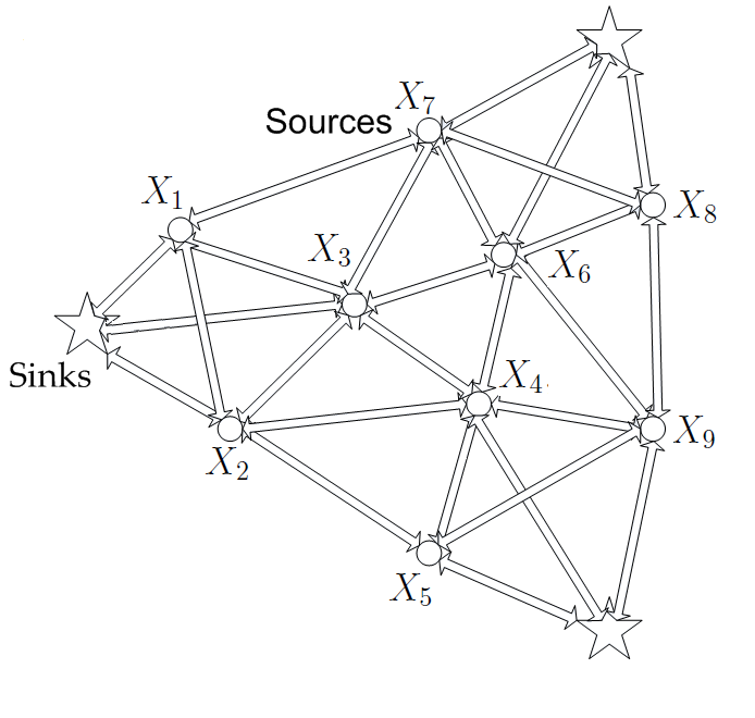
Figure 1: A general multi-source multi-sink sensor network. The circles denote sources and stars denote sinks. The arrows denote allowed communication links.

This paper focuses on minimum cost communication of correlated sources over a network with multiple-sinks. We introduce a new routing paradigm called Dispersive Information Routing (DIR), wherein intermediate nodes are allowed to “split a packet” and forward a subset of the received bits on each of the forward paths. This paradigm opens up a rich class of research problems which focus on the interplay between encoding and routing in a network. What makes it particularly interesting is the challenge in encoding sources such that exactly the required information is routed to each sink, to reconstruct the prescribed subset of sources. We will show, using simple examples that asymptotically, DIR achieves a lower cost over conventional routing methods, wherein the sinks usually receive more information than they need. This paradigm leads to a general class of information theoretic problems, which have not been studied earlier. In this paper, we formulate this problem and the associated rate region. We introduce a new (random) coding technique using principles from multiple descriptions encoding and Han and Kobayashi decoding, which leads to an achievable rate region for this problem. We show that this achievable rate region is complete under certain special scenarios.

The rest of the paper is organized as follows. In Section II, we review prior work related to distributed source coding and network routing. Before stating the problem formally, in Section III, we provide 2 simple examples to demonstrate the basic principles behind DIR and the new encoding scheme. We also demonstrate the suboptimality of conventional routing methods using these simple examples. In Section IV, we formally state the DIR problem and provide an achievable rate region. Finally, in Section V, we show that this achievable rate region is complete for some special cases of the setup.

II Prior Work

Multi-terminal source coding has one of its early roots in the seminal work of Slepian and Wolf [4]. They showed, in the context of lossless coding, that side-information available only at the decoder can nevertheless be fully exploited as if it were available to the encoder, in the sense that there is no asymptotic performance loss. Later, Wyner and Ziv [5] derived a lossy coding extension that bounds the rate-distortion performance in the presence of decoder side information. Extensive work followed considering different network scenarios and obtaining achievable rate regions for them, including [6, 7, 8, 9, 10, 11, 12, 13, 14]. Han and Kobayashi [3] extended the Slepian-Wolf result to general multi-terminal source coding scenarios. For a multi-sink network, with each sink reconstructing a prespecified subset of the sources, they characterized an achievable rate region for lossless reconstruction of the required sources at each sink. Csisz$\mathrm{\acute{a}}$r and K$\mathrm{\ddot{o}}$rner [15] provided an alternative characterization of the achievable rate region for the same setup by relating the region to the solution of a class of problems called the “entropy characterization problems”.

There has also been a considerable amount of work on joint compression-routing for networks. A survey of routing techniques for sensor networks is given in [16]. It was shown in [17] that the problem of finding the optimum route for compression using explicit communication is an NP-complete problem. [18] compared different joint compression-routing schemes for a correlated sensor grid and also proposed an approximate, practical, static source clustering scheme to achieve compression efficiency. Much of the above work is related to compression using explicit communication, without recourse to distributed source coding techniques. Cristescu et al. [1] considered joint optimization of Slepian-Wolf coding and a routing mechanism, we call ‘broadcasting’, wherein each source broadcasts its information to all sinks that intend to reconstruct it. Such a routing mechanism is motivated from the extensive literature on optimal routing for independent sources [19]. [20] proved the general optimality of that approach for networks with a single sink. We demonstrated its sub-optimality for the multi-sink scenario, recently in [21]. This paper takes a step further towards finding the best joint compression-routing mechanism for a multi-sink network. We note that a preliminary version of our results appeared in [22] and [23].

We note the existence of a volume of work on minimum cost network coding for correlated sources, e.g. [24, 25]. But the routing mechanism we introduce in this paper does not require possibly complex network coders at intermediate nodes, and can be realized using simple conventional routers. The approach does have potential implications on network coding, but these are beyond the scope of this paper.

III Dispersive Information Routing - Simple Networks

III-A Basic Notation

We begin by introducing the basic notation. In what follows, $2^{\mathcal{S}}$ denotes the set of all subsets (power set) of any set $\mathcal{S}$ and $|\mathcal{S}|$ denotes the set cardinality. Note that $|2^{\mathcal{S}}|=2^{|\mathcal{S}|}$. $\mathcal{S}^{c}$ denotes the set complement (the universal set will be specified when there is ambiguity) and $\phi$ denotes the null set. For two sets $\mathcal{S}_{1}$ and $\mathcal{S}_{2}$, we denote the set difference by $\mathcal{S}_{1}-\mathcal{S}_{2}=\{s:s\in\mathcal{S}_{1},s\notin\mathcal{S}_{2}\}$. Random variables are denoted by upper case letters (for example $X$) and their realizations are denoted by lower case letters (for example $x$). We also use upper case letters to denote source nodes and sinks and the ambiguity will be clarified wherever necessary. A sequence of $n$ independent and identically distributed (iid) random variables and its realization are denoted by $X^{n}$ and $x^{n}$, respectively. The length $n$, $\epsilon$-typical set is denoted by $\mathcal{T}_{\epsilon}^{n}$. $X\leftrightarrow Y\leftrightarrow Z$ denotes that the three random variables $(X,Y,Z)$ form a Markov chain in that order. Notation in [26] is used to denote standard information theoretic quantities.

III-B Illustrative example - No helpers case

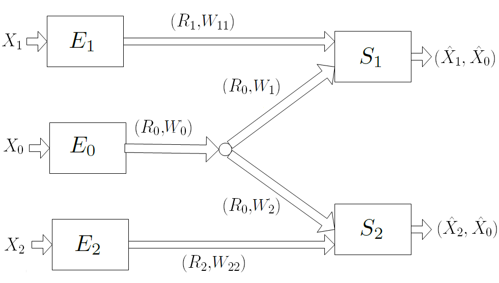
Figure 2: Example 1 - Conventional Routing

Consider the network shown in Fig. 2. There are three source nodes, $E_{0}$, $E_{1}$ and $E_{2}$ and two sinks $S_{1}$ and $S_{2}$. The three source nodes observe correlated memoryless sequences $X_{0}^{n},X_{1}^{n}$ and $X_{2}^{n}$, respectively. Sink $S_{1}$ reconstructs the pair $(X_{0}^{n},X_{1}^{n})$, while $S_{2}$ reconstructs $(X_{0}^{n},X_{2}^{n})$. $E_{0}$ communicates with the two sinks through an intermediate node (called the ‘collector’) which is functionally a simple router. The edge weights on each path in the network are as shown in the figure. The cost of communication through an edge, $e$, is a function of the bit rate flowing through it, denoted by $R_{e}$ and the corresponding edge weight, denoted by $W_{e}$, which in this paper, we will assume for simplicity to be a simple product $C(R_{e},W_{e})=R_{e}W_{e}$, noting that the approach is directly extendible to more complex cost functions. We further assume that the total cost is the sum of individual communication cost over each edge. The objective is to find the minimum total communication cost for lossless transmission of sources to the respective sinks.

We first consider the communication cost when broadcast routing is employed [1] wherein the routers forward all the bits received from a source to all the decoders that would reconstruct it. In other words, routers are not allowed to “split” a packet and forward a portion of the received information on the forward paths. Hence the branches connecting the collector to the two sinks carry the same rates as the branch connecting $E_{0}$ to the collector. We denote the rate at which $X_{0}$, $X_{1}$ and $X_{2}$ are encoded by $R_{0}$, $R_{1}$ and $R_{2}$, respectively.

Using results in [1], it can be shown that the minimum communication cost under broadcast routing is given by the solution to the following linear programming formulation:

$$C_{br}=\min\{(W_{0}+W_{1}+W_{2})R_{0}+W_{11}R_{1}+W_{22}R_{2}\}$$ (1)

under the constraints:

$$R_{0} \geq \max(H(X_{0}|X_{1}),H(X_{0}|X_{2}))$$

$$R_{1} \geq H(X_{1}|X_{0})$$

$$R_{2} \geq H(X_{2}|X_{0})$$

$$R_{1}+R_{0} \geq H(X_{0},X_{1})$$

$$R_{2}+R_{0} \geq H(X_{0},X_{2})$$ (2)

To gain intuition into dispersive information routing, we will later consider a special case of the above network when the branch weights are such that $W_{11},W_{22}\ll W_{0},W_{1},W_{2}$. Let us specialize the above equations for this case. The constraint $W_{11},W_{22}\ll W_{0},W_{1},W_{2}$, implies that $X_{1}$ and $X_{2}$ should be encoded at rates $R_{1}=H(X_{1})$ and $R_{2}=H(X_{2})$, respectively. Therefore the scenario effectively captures the case when $X_{1}$ and $X_{2}$ are available as side information at the respective decoders. It follows from (1) and (2) that for achieving minimum communication cost, $R_{0}$ is:

$$R_{0}^{*}=\max\left\{H(X_{0}|X_{1}),H(X_{0}|X_{2})\right\}$$ (3)

and therefore the minimum communication cost is given by:

$$C_{br}^{*} = (W_{0}+W_{1}+W_{2})R_{0}^{*}$$ (4)

$$+W_{11}H(X_{1})+W_{22}H(X_{2})$$

Is this the best we can do? The collector has to transmit enough information to sink $S_{1}$ for it to decode $X_{0}$ and therefore the rate is at least $H(X_{0}|X_{1})$. Similarly the rate on the branch connecting the collector to $S_{2}$ is at least $H(X_{0}|X_{2})$. But if $H(X_{0}|X_{1})\neq H(X_{0}|X_{2})$, there is excess rate on one of the branches.

Let us now relax this restriction and allow the collector node to “split” the packet and route different subsets of the received bits on the forward paths. We could equivalently think of the source $E_{0}$ transmitting 3 smaller packets to the collector; the first packet has a rate $R_{0,\{1,2\}}$ bits and is destined to both sinks. Two other packets have rates $R_{0,1}$ and $R_{0,2}$ and are destined to sinks $S_{1}$ and $S_{2}$, respectively. Technically, in this case, the collector is again a simple conventional router.

We refer to such a routing mechanism, where each intermediate node transmits a subset of the received bits on each of the forward paths, as “Dispersive Information Routing” (DIR). Note that unlike network coding, DIR does not require possibly expensive coders at intermediate nodes, and can always be realized using conventional routers, with each source transmitting multiple packets into the network intended to different subsets of sinks. Hereafter, we interchangeably use the ideas of “packet splitting” at intermediate nodes and conventional routing of smaller packets, noting the equivalence in achievable rates and costs. This scenario is depicted in Fig. 3 with the modified cost each packet encounters.

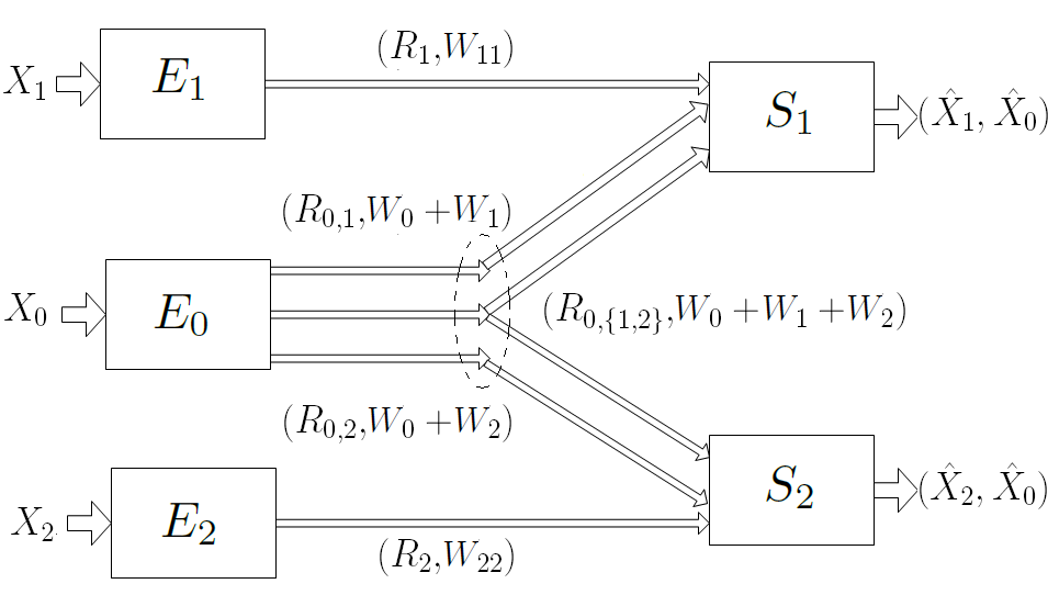
Figure 3: Example - DIR. Note that the notion of ‘packet splitting’ is equivalent to the sources transmitting multiple smaller packets

Two obvious questions arise - Does DIR achieve a lower communication cost compared to conventional routing? If so, what is the minimum communication cost under DIR?

We first aim to find the minimum cost using DIR under the special case of $W_{11},W_{22}\ll W_{0},W_{1},W_{2}$ (i.e., $R_{1}=H(X_{1})$ and $R_{2}=H(X_{2})$). To establish the minimum communication cost we need to first establish the complete achievable rate region for the rate tuple $\{R_{0,1},R_{0,\{1,2\}},R_{0,2}\}$ for lossless reconstruction of $X_{0}^{n}$ at both the decoders and then find the point in the achievable rate region that minimizes the total communication cost, determined using the modified weights shown in Fig. 3. Before deriving the ultimate solution, it is instructive to consider one operating point, $P_{1}\triangleq\{R_{0,1},R_{0,\{1,2\}},R_{0,2}\}=\{I(X_{1};X_{0}|X_{2}),H(X_{0}|X_{1},X_{2}),I(X_{2};X_{0}|X_{1})\}$ and provide the coding scheme that achieves it. Extension to other “interesting points” and to the whole achievable region follows in similar lines. This particular rate point is considered first due to its intuitive appeal as shown in a Venn diagram (Fig. 4a).

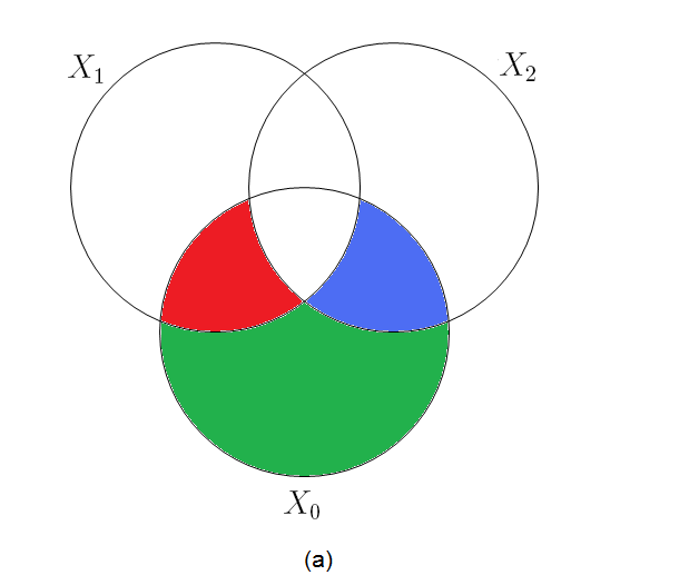
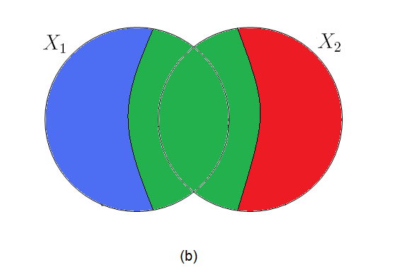
Figure 4: Venn Diagram based intuition: (a) Amount of information routed using DIR when operating at point $P_{1}$. Observe that each of the sinks receive information at the respective minimum rates. Green represents $R_{0,12}$, Blue represents $R_{0,1}$ and Red represents $R_{0,2}$ (b) Intuitive representation of Wyner’s common information. Observe that in Wyner’s setup, it is generally not possible to split the information exactly and that there is a rate loss due to transmitting the common bit stream.

Gray and Wyner considered a closely resembling network [13] shown in Fig. 5. In their setup, the encoder observes iid sequences of $2$ correlated random variables $(X_{1},X_{2})$ and transmits $3$ packets (at rates $R_{0,1},R_{0,\{1,2\}},R_{0,2}$, respectively), one meant for each subset of sinks. The two sinks reconstruct sequences $X_{1}^{n}$ and $X_{2}^{n}$, respectively. They showed that the rate tuple $\{R_{0,1},R_{0,\{1,2\}},R_{0,2}\}=\{H(X_{1}|X_{2}),I(X_{1};X_{2}),H(X_{2}|X_{1})\}$ is not achievable in general and that there is a rate loss due to transmitting a common bit stream; in the sense that individual decoders must receive more information than they need to reconstruct their respective sources if the sum rate is maintained at minimum. Wyner defined the term “Common Information” [11], here denoted by $C_{W}(X_{1};X_{2})$ as the minimum rate $R_{0,\{1,2\}}$ such that $\{R_{0,1},R_{0,\{1,2\}},R_{0,2}\}$ is achievable and $R_{0,1}+R_{0,\{1,2\}}+R_{0,2}=H(X_{1},X_{2})$. He also showed that $C(X_{1};X_{2})=\min I(X_{1},X_{2};U)$ where the $\min$ is taken over all auxiliary random variables $U$ such that $X_{1}\leftrightarrow U\leftrightarrow X_{2}$ form a Markov chain. He further showed that, in general, $I(X_{1};X_{2})\leq C_{w}(X_{1};X_{2})\leq\max(H(X_{1}),H(X_{2}))$. We note in passing, the existence of an earlier definition of common information by G$\mathrm{\acute{a}}$cs and K$\mathrm{\ddot{o}}$rner [27] which measures the maximum shared information that can be fully utilized by both the decoders. It is less relevant to dispersive information routing.

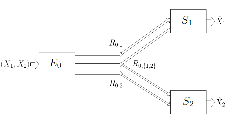
Figure 5: Gray-Wyner Setup. Note the resemblance to the DIR setup in Fig. 3

At first glance, it might be tempting to extend Wyner’s argument to the DIR setting and say $P_{1}$ is not achievable in general, i.e., each decoder has to receive more information than it needs. But interestingly enough, a rather simple coding scheme achieves this point and simple extensions of the coding scheme can achieve the entire rate region for this example. The primary difference between Gray-Wyner network and DIR is that in their setup two correlated sources are encoded jointly for separate decoding at each sink. However, in our setup, $X_{0}^{n}$ is encoded for lossless decoding at both the sinks. Note that this section only provides intuitive arguments to support the result. A coding scheme will be formally derived in section IV, for the general setup.

We concentrate on encoding at $E_{0}$ assuming that $E_{1}$ and $E_{2}$ transmit at their respective source entropies. $E_{0}$ observes a sequence of $n$ iid random variables $X_{0}^{n}$. This sequence belongs to the typical set, $\mathcal{T}_{\epsilon}^{n}$, with high probability. Every typical sequence is assigned $3$ indices, each independent of the other. The three indices are assigned using uniform pmfs over $[1:2^{nR_{{}_{0,1}}}]$, $[1:2^{nR_{0,\{1,2\}}}]$ and $[1:2^{nR_{0,2}}]$, respectively. All the sequences with the same first index, $m_{0,1}$, form a bin $\mathcal{B}_{0,1}(m_{0,1})$. Similarly bins $\mathcal{B}_{0,2}(m_{0,2})$ and $\mathcal{B}_{0,12}(m_{0,12})$ are formed for all indices $m_{0,2}$ and $m_{0,12}$, respectively. Upon observing a sequence $x_{0}^{n}\in\mathcal{T}_{\epsilon}^{n}$ with indices $m_{0,1},m_{0,2}$ and $m_{0,12}$, the encoder transmits index $m_{0,1}$ to decoder $1$ alone, index $m_{0,2}$ to decoder $2$ alone and index $m_{0,12}$ to both the decoders.

The first decoder receives indices $m_{0,1}$ and $m_{0,12}$. It tries to find a typical sequence $\hat{x}_{0}^{n}\in\mathcal{B}_{0,1}(m_{0,1})\cap\mathcal{B}_{0,12}(m_{0,12})$ which is jointly typical with the decoded information sequence $x_{1}^{n}$. As the indices are assigned independent of each other, every typical sequence has uniform pmf of being assigned to the index pair $\{m_{0,1},m_{0,12}\}$ over $[1:2^{n(R_{0,1}+R_{0,\{1,2\}})}]$. Therefore, having received indices $m_{0,1}$ and $m_{0,12}$, using arguments similar to Slepian-Wolf [4] and Cover [7], the probability of decoding error asymptotically approaches zero if:

$$R_{0,1}+R_{0,\{1,2\}}\geq H(X_{0}|X_{1})$$ (5)

Similarly, probability of decoding error approaches zero at the second decoder if:

$$R_{0,2}+R_{0,\{1,2\}}\geq H(X_{0}|X_{2})$$ (6)

Clearly (5) and (6) imply that $P_{1}$ is achievable. In similar lines to [4, 7], the above achievable region can also be shown to satisfy the converse and hence is the complete achievable rate region for this problem. We term such a binning approach as ‘Power Binning’ as an independent index is assigned to each (non-trivial) subset of the decoders - the power set. It is worthwhile to note that the same rate region can be obtained by applying results of Han and Kobayashi [3], assuming 3 independent encoders at $E_{0}$, albeit with a more complicated coding scheme involving multiple auxiliary random variables (see also [28]). We also note that the mechanism of assigning multiple independent random bin indices has been used is several related prior work, such as [29, 30].

The minimum cost operating point is the point that satisfies equations (5) and (6) and minimizes the cost function:

$$C_{DIR-SI}^{*} = \min\,\,\,\,\{(W_{0}+W_{1})R_{0,1}+(W_{0}+W_{2})R_{0,2}$$ (7)

$$+(W_{0}+W_{1}+W_{2})R_{0,\{1,2\}}\}$$

The solution is either one of the two points $P_{2}\triangleq\{0,H(X_{0}|X_{1}),H(X_{0}|X_{2})-H(X_{0}|X_{1})\}$ or $P_{3}\triangleq\{H(X_{0}|X_{1})-H(X_{0}|X_{2}),H(X_{0}|X_{2}),0\}$ and both achieve lower total communication cost compared to broadcast routing, $C_{conv}^{*}$ in (4), for any $W_{0},W_{1},W_{2}\gg W_{11},W_{22}$ if $H(X_{0}|X_{1})\neq H(X_{0}|X_{2})$.

The above coding scheme can be easily extended to the case of arbitrary edge weights. Then, the rate region for the tuple $\{R_{1},R_{2},R_{0,1},R_{0,\{1,2\}},R_{0,2}\}$ and the cost function to be minimized are given by:

$$C_{DIR}^{*}=\min\,\,\,\,\{W_{11}R_{1}+W_{22}R_{2}+(W_{0}+W_{1})R_{0,1}$$

$$+(W_{0}+W_{2})R_{0,2}+(W_{0}+W_{1}+W_{2})R_{0,\{1,2\}}\}$$ (8)

under the constraints:

$$R_{1} \geq H(X_{1}|X_{0})$$

$$R_{0,1}+R_{0,\{1,2\}} \geq H(X_{0}|X_{1})$$

$$R_{1}+R_{0,1}+R_{0,\{1,2\}} \geq H(X_{0},X_{1})$$

$$R_{2} \geq H(X_{2}|X_{0})$$

$$R_{0,2}+R_{0,\{1,2\}} \geq H(X_{0}|X_{2})$$

$$R_{2}+R_{0,2}+R_{0,\{1,2\}} \geq H(X_{0},X_{2})$$ (9)

If $R_{1}=H(X_{1})$ and $R_{2}=H(X_{2})$, (9) specializes to (5) and (6). Also, it can easily be shown that the total communication cost obtained as a solution to the above formulation is lower than that for conventional routing if $W_{0},W_{1},W_{2}>0$. This example clearly demonstrates the gains of DIR over broadcast routing to communicate correlated sources over a network.

Observe that in the above example, the sinks only receive information from the source nodes they intend to reconstruct. Such a scenario is called the ‘No helpers’ case in the literature [15]. In a network with multiple sources and sinks, if source $i$ is to be reconstructed at a subset of sinks $\Pi_{i}$, power binning assigns $2^{|\Pi_{i}|}-1$ independently generated indices, each being routed to a subset of $\Pi_{i}$. It will be shown later in section V that power binning achieves minimum cost under DIR, even for a general setup, as long as there are no helpers, i.e., when each sink is allowed to receive information only from the requested sources. However, the problem of establishing the complete achievable rate region becomes considerably harder when every source is allowed to communicate with every sink, a scenario, that is highly relevant to practical networks. It was shown in [21] that for certain networks, unbounded gains in communication cost are obtained when source nodes are allowed to communicate with sinks that do not reconstruct them. In this paper, we derive an achievable rate region for this setup. In the following subsection, to keep the notations and understanding simple, we begin with one of the simplest setups which illustrates the underlying ideas.

III-C A simple network with helpers

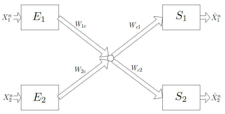
Figure 6: The 2 Source - 2 Sink example. Each source acts as the principle source for one sink and as a helper for the other

We will again provide only intuitive description for the encoding scheme here and defer the formal proofs for the general case to section IV. Consider the network shown in Fig. 6. Two source nodes $E_{1}$ and $E_{2}$ observe correlated memoryless sequences $X_{1}^{n}$ and $X_{2}^{n}$, respectively. Two sinks $S_{1}$ and $S_{2}$ require lossless reconstructions of $X_{1}^{n}$ and $X_{2}^{n}$, respectively. The source nodes can communicate with the sinks only through a collector node. The edge weights are as shown in the figure. Observe that, each source, while requested by one sink, acts as helper for the other.

Under dispersive information routing, each source transmits a packet to every subset of sinks. In this example, $E_{1}$ sends 3 packets to the collector at rates $(R_{1,1},R_{1,2},R_{1,12})$, respectively. The collector forwards the first packet to $S_{1}$, the second to $S_{2}$ and the third to both $S_{1}$ and $S_{2}$. Similarly, $E_{2}$ sends 3 packets to the collector at rates $(R_{2,1},R_{2,2},R_{2,12})$ which are forwarded to the corresponding sinks. Our objective is to determine the set of achievable rate tuples $(R_{1,1},R_{1,2},R_{1,12},R_{2,1},R_{2,2},R_{2,12})$ that allows for lossless reconstruction at the two sinks. The minimum cost then follows by finding the point in the achievable rate region which minimizes the effective communication cost, $C_{DIR}$, given by:

$$\sum_{i=1}^{2}(W_{ic}+W_{c1}+W_{c2})R_{i,12}+(W_{2c}+W_{c1})R_{2,1}$$

$$+\sum_{i=1}^{2}(W_{ic}+W_{ci})R_{i,i}+(W_{1c}+W_{c2})R_{1,2}$$ (10)

A non-single letter characterization of the complete rate region is possible using the results of Han and Kobayashi in [3]. They also provide a single-letter partial achievable rate region. However, applicability of their result requires artificial imposition of 3 independent encoders at each source, which is an unnecessary restriction. We present a more general achievable rate region, which maintains the dependencies between the messages at each encoder. Note that the source coding setup which arises out of the DIR framework is a special case of the general problem of distributed multiple descriptions and therefore the principles underlying the coding schemes for distributed source coding [3] and multiple descriptions encoding [2] play crucial roles in deriving a coding mechanism for dispersive information routing. It is interesting to observe that, unlike the general MD setting, the DIR framework is non-trivial even in the lossless scenario and deriving a complete rate region for lossless reconstruction at all the sinks is a challenging problem.

We now give an achievable region for the example in Fig. 6. Suppose we are given random variables $(U_{1,12},U_{1,1},U_{1,2},U_{2,12},U_{2,1},U_{2,2})$ jointly distributed with $(X_{1},X_{2})$ such that the following Markov chain conditions hold:

$$(U_{1,12},U_{1,1}) \leftrightarrow X_{1}\leftrightarrow X_{2}\leftrightarrow(U_{2,12},U_{2,1})$$

$$(U_{1,12},U_{1,2}) \leftrightarrow X_{1}\leftrightarrow X_{2}\leftrightarrow(U_{2,12},U_{2,2})$$ (11)

Note that the codeword indices of $U_{i,\mathcal{S}}$ are sent in the packet from source $E_{i}$ to sinks $S_{j}:j\in\mathcal{S}$. The encoding is divided into 3 stages.

Encoding : We first focus on the encoding at $E_{1}$. In the first stage, $2^{nR_{1,12}^{{}^{\prime}}}$ codewords of $U_{1,12}$, each of length $n$ are generated independently, with elements drawn according to the marginal density $P(U_{1,12})$. Conditioned on each of these codewords, $2^{nR_{1,1}^{{}^{\prime}}}$ and $2^{nR_{1,2}^{{}^{\prime}}}$ codewords of $U_{1,1}$ and $U_{1,2}$ are generated according to the conditional densities $P(U_{1,1}|U_{1,12})$ and $P(U_{1,2}|U_{1,12})$, respectively. Codebooks for $U_{2,12},U_{2,1}$ and $U_{2,2}$ are generated at $E_{2}$ in a similar fashion. On observing a sequence $x_{1}^{n}$, $E_{1}$ first tries to find a codeword tuple from the codebooks of $(U_{1,12},U_{1,1},U_{1,2})$ such that $(x_{1}^{n},u_{1,12}^{n},u_{1,1}^{n})\in\mathcal{T}_{\epsilon}^{n}$ and $(x_{1}^{n},u_{1,12}^{n},u_{1,2}^{n})\in\mathcal{T}_{\epsilon}^{n}$. The probability of finding such a codeword tuple approaches 1 if,

$$R_{1,12}^{{}^{\prime}} \geq I(X_{1};U_{1,12})$$

$$R_{1,1}^{{}^{\prime}} \geq I(X_{1};U_{1,1}|U_{1,12})$$

$$R_{1,2}^{{}^{\prime}} \geq I(X_{1};U_{1,2}|U_{1,12})$$ (12)

Let the codewords selected be denoted by ($u_{1,12},$$u_{1,1}$,$u_{1,2}$). Similar constraints on $(R_{2,1}^{{}^{\prime}},R_{2,2}^{{}^{\prime}},R_{2,12}^{{}^{\prime}})$ must be satisfied for encoding at $E_{2}$. Denote the codewords selected at $E_{2}$ by $(u_{2,12},u_{2,1},u_{2,2})$. It follows from (11) and the ‘Conditional Markov Lemma’ in [10] that $(x_{1}^{n},x_{2}^{n},u_{1,12},u_{1,1},u_{2,12},u_{2,1})\in\mathcal{T}_{\epsilon}^{n}$ and $(x_{1}^{n},x_{2}^{n},u_{1,12},u_{1,2},u_{2,12},u_{2,2})\in\mathcal{T}_{\epsilon}^{n}$ with high probability.

In the second stage of encoding, each encoder uniformly divides the $2^{nR_{i,\mathcal{S}}^{{}^{\prime}}}$ codewords of $U_{i,\mathcal{S}}$ into $2^{nR_{i,\mathcal{S}}^{{}^{\prime\prime}}}$ bins $\forall\,i\in\{1,2\}$, $\mathcal{S}\in\{1,2,12\}$. All the codewords which have the same bin index $m$ are said to fall in the bin $\mathcal{C}_{i,\mathcal{S}}(m)$ $\forall m\in(1\ldots 2^{nR_{i,\mathcal{S}}^{{}^{\prime\prime}}})$. Note that the number of codewords in bin $\mathcal{C}_{i,\mathcal{S}}(m)$ is $2^{n(R_{i,\mathcal{S}}^{{}^{\prime}}-R_{i,\mathcal{S}}^{{}^{\prime\prime}})}$. If $E_{1}$ selects the codewords $(u_{1,12},u_{1,1},u_{1,2})$ in the first stage and if the bin indices associated with $(u_{1,12},u_{1,1},u_{1,2})$ are $(m_{1,12},m_{1,1},m_{1,2})$, then index $m_{1,1}$ is routed to sink $S_{1}$, $m_{1,2}$ to sink $S_{2}$ and $m_{1,12}$ to both the sinks $S_{1}$ and $S_{2}$. Similarly, bin indices $(m_{2,12},m_{2,1},m_{2,2})$ are routed from $E_{2}$ to the corresponding sinks.

The third stage of encoding, resembles the ‘Power Binning’ scheme described in Section III-B. Every typical sequence of $X_{1}^{n}$ is assigned a random bin index uniformly chosen over $[1:2^{n\tilde{R}_{1,1}}]$. All sequences with the same index, $l_{1,1}$, form a bin $\mathcal{B}_{1,1}(l_{1,1})$ $\forall l_{1,1}\in\{1\ldots 2^{n\tilde{R}_{1,1}}\}$. Upon observing a sequence $X_{1}^{n}\in\mathcal{T}_{\epsilon}^{n}$ with bin index $l_{1,1}$, in addition to $m_{1,1}$ (from the second stage of encoding), encoder $E_{1}$ also routes index $l_{1,1}$ to sink $S_{1}$. Similarly bin index $l_{2,2}$ is routed from $E_{2}$ to $S_{2}$ in addition to $m_{2,2}$. These bin indices are used to reconstruct $X_{1}^{n}$ and $X_{2}^{n}$ losslessly at the respective decoders. Note that, in a general setup, if source $i$ is to be reconstructed at a subset of sinks $\Pi_{i}$, the source assigns $2^{|\Pi_{i}|}-1$ independently generated indices, each being routed to a subset of $\Pi_{i}$. We also note that $U_{1,1}$ and $U_{2,2}$ can be conveniently set to constants without changing the overall rate region. However, we continue to use them to avoid complex notation.

Decoding : We again focus on the first sink $S_{1}$. It receives the indices $(m_{1,12},m_{1,1},m_{2,12},m_{2,1},l_{1,1})$. It first looks for a pair of unique codewords from $\mathcal{C}_{1,12}(m_{1,12})$ and $\mathcal{C}_{2,12}(m_{2,12})$ which are jointly typical. Obviously, there is at least one pair, $(u_{1,12},u_{2,12})$, which is jointly typical. The probability that no other pair of codewords are jointly typical approaches $1$ if:

$$(R_{1,12}^{{}^{\prime}}-R_{1,12}^{{}^{\prime\prime}})+(R_{2,12}^{{}^{\prime}}-R_{2,12}^{{}^{\prime\prime}})\leq I(U_{1,12};U_{2,12})$$ (13)

Noting that $(R_{1,12}^{{}^{\prime}}-R_{1,12}^{{}^{\prime\prime}})\geq 0$ and $(R_{2,12}^{{}^{\prime}}-R_{2,12}^{{}^{\prime\prime}})\geq 0$, and applying the constraints on $R_{1,12}^{{}^{\prime}}$ and $R_{2,12}^{{}^{\prime}}$ from (12) we get the following constraints for $R_{1,12}^{{}^{\prime\prime}}$ and $R_{2,12}^{{}^{\prime\prime}}$:

$$R_{1,12}^{{}^{\prime\prime}} \geq I(X_{1};U_{1,12}|U_{2,12})$$

$$R_{2,12}^{{}^{\prime\prime}} \geq I(X_{2};U_{2,12}|U_{1,12})$$

$$R_{1,12}^{{}^{\prime\prime}}+R_{2,12}^{{}^{\prime\prime}} \geq I(X_{1},X_{2};U_{1,12},U_{2,12})$$ (14)

The decoder at $S_{1}$ next looks at the codebooks of $U_{1,1}$ and $U_{2,1}$ which were generated conditioned on $u_{1,12}$ and $u_{2,12}$, respectively, to find a unique pair of codewords from $\mathcal{C}_{1,1}(m_{1,1})$ and $\mathcal{C}_{2,1}(m_{2,1})$ which are jointly typical with $(u_{1,12},u_{2,12})$. We again have one pair, $(u_{1,1},u_{2,1})$, which is jointly typical with $(u_{1,12},u_{2,12})$. It can be shown using arguments similar to [3] that the probability of finding no other jointly typical pair approaches $1$ if :

$$(R_{1,1}^{{}^{\prime}}-R_{1,1}^{{}^{\prime\prime}}) \leq I(U_{1,1};U_{2,1},U_{2,12}|U_{1,12})$$

$$(R_{2,1}^{{}^{\prime}}-R_{2,1}^{{}^{\prime\prime}}) \leq I(U_{2,1};U_{1,1},U_{1,12}|U_{2,12})$$

$$\bigl{\{}(R_{1,1}^{{}^{\prime}}-R_{1,1}^{{}^{\prime\prime}}) \leq H(U_{1,1}|U_{1,12})+H(U_{2,1}|U_{2,12})$$

$$+(R_{2,1}^{{}^{\prime}}-R_{2,1}^{{}^{\prime\prime}})\bigr{\}} -H(U_{1,1},U_{2,1}|U_{1,12},U_{2,12})$$ (15)

On substituting the constraints for $R_{1,1}^{{}^{\prime}}$ and $R_{1,2}^{{}^{\prime}}$ from (12), and using the Markov chain condition in (11) we get:

$$R_{1,1}^{{}^{\prime\prime}} \geq I(X_{1};U_{1,1}|U_{1,12},U_{2,12},U_{2,1})$$

$$R_{2,1}^{{}^{\prime\prime}} \geq I(X_{2};U_{2,1}|U_{1,12},U_{2,12},U_{1,1})$$

$$R_{1,1}^{{}^{\prime\prime}}+R_{2,1}^{{}^{\prime\prime}} \geq I(X_{1},X_{2};U_{1,1},U_{2,1}|U_{1,12},U_{2,12})$$ (16)

After successfully decoding the codewords $(u_{1,12},u_{1,1},u_{2,12},u_{2,1})$, the decoder at $S_{1}$ looks for a unique sequence from $\mathcal{B}_{1,1}(l_{1,1})$ which is jointly typical with $(u_{1,12},u_{1,1},u_{2,12},u_{2,1})$. We again have $x_{1}^{n}$ satisfying this property. It can be shown that the probability of finding no other sequence which is jointly typical with $(u_{1,12},u_{1,1},u_{2,12},u_{2,1})$ approaches $1$ if:

$$\tilde{R}_{1,1}\geq H(X_{1}|U_{1,12},U_{2,12},U_{1,1},U_{2,1})$$ (17)

Similar conditions at sink $S_{2}$ lead to the following constraints:

$$R_{2,2}^{{}^{\prime\prime}} \geq I(X_{2};U_{2,2}|U_{1,12},U_{2,12},U_{1,2})$$

$$R_{1,2}^{{}^{\prime\prime}} \geq I(X_{2};U_{1,2}|U_{1,12},U_{2,12},U_{2,2})$$

$$R_{2,2}^{{}^{\prime\prime}}+R_{1,2}^{{}^{\prime\prime}} \geq I(X_{1},X_{2};U_{2,2},U_{1,2}|U_{1,12},U_{2,12})$$

$$\tilde{R}_{2,2} \geq H(X_{2}|U_{1,12},U_{2,12},U_{1,2},U_{2,2})$$ (18)

The first packet from $E_{1}$, destined to only $S_{1}$, carries indices $(m_{1,1},l_{1,1})$ at rate $R_{1,1}=R_{1,1}^{{}^{\prime\prime}}+\tilde{R}_{1,1}$. The second and third packets carry $m_{1,2}$ and $m_{1,12}$ at rates $R_{1,2}=R_{1,2}^{{}^{\prime\prime}}$ and $R_{1,12}=R_{1,12}^{{}^{\prime\prime}}$, respectively and are routed to the corresponding sinks. Similarly, 3 packets are transmitted from $E_{2}$ carrying indices $\{m_{2,1},m_{2,12},(m_{2,2},l_{2,2})\}$ at rates $(R_{2,1},R_{2,12},R_{2,2})=(R_{2,1}^{{}^{\prime\prime}},R_{2,12}^{{}^{\prime\prime}},R_{2,2}^{{}^{\prime\prime}}+\tilde{R}_{2,2})$ to sinks $\{S_{1},S_{2},(S_{1},S_{2})\}$, respectively. Constraints for $(R_{1,1},R_{1,2},R_{1,12},R_{2,1},R_{2,2},R_{2,12})$ can now be obtained using (14),(16), (17) and (18). The convex closure of achievable rates over all such random variables $(U_{1,12},U_{1,1},U_{1,2},U_{2,12},U_{2,1},U_{2,2})$ gives the achievable rate region for the 2 source - 2 sink DIR problem. It is easy to verify that this region subsumes the region that would be produced by employing the approach of Han and Kobayashi [3], which must assume three independent encoders at each source. Observe that in the above illustration, we assumed that the decoding is performed in a sequential manner, i.e., the codewords of $U_{1,12}$ are decoded first followed by the codewords of $(U_{1,1})$ and $(U_{1,2})$, respectively. This was done only for the ease of understanding. In Theorem 1, we derive the conditions on rates for the decoders to find typical sequences from all the codebooks jointly (at once). Note that conditions on the rates for joint decoding is generally weaker (the region is larger) than that for sequential decoding.

IV Dispersive Information Routing - General Setup

Let a network be represented by an undirected connected graph $G=(V,\mathcal{E})$. Each edge $e\in\mathcal{E}$ is associated with an edge weight, $W_{e}$. The communication cost is assumed to be a simple product of the edge rate and edge weight, i.e., $C_{e}=R_{e}W_{e}$. The nodes $V$ consist of $N$ source nodes (denoted by $E_{1},E_{2}\ldots E_{N}$), $M$ sinks (denoted by $S_{1},S_{2}\ldots S_{M}$), and $|V|\text{\textminus}N\text{\textminus}M$ intermediate nodes. We define the sets $\Sigma=\{1\ldots N\}$ and $\Pi=\{1\ldots M\}$. Source node $E_{i}$ observes $n$ iid random variables $X_{i}^{n}$, each taking values over a finite alphabet $\mathcal{X}_{i}$. Sink $S_{j}$ reconstructs (requests) a subset of the sources specified by $\Sigma_{j}\subseteq\Sigma$. Conversely, source node $E_{i}$ is reconstructed at a subset of sinks specified by $\Pi_{i}\subseteq\Pi$. The objective is to find the minimum communication cost achievable by dispersive information routing for lossless reconstruction of the requested sources at each sink when every source node can (possibly) communicate with every sink.

IV-A Obtaining the effective costs

Under DIR each source transmits at most $2^{M}-1$ packets into the network, each meant for a different subset of sinks. Note that, while $\Pi_{i}$ is the subset of sinks reconstructing $X_{i}^{n}$, $E_{i}$ may be transmitting packets to many other subsets of sinks. Let the packet from source $E_{i}$ to the subset of sinks $\mathcal{K}\subseteq\Pi$ be denoted by $\mathcal{P}_{i,\mathcal{K}}$ and let it carry information at rate $R_{i,\mathcal{K}}$.

The optimum route for packet $\mathcal{P}_{i,\mathcal{K}}$ from the source to these sinks is determined by a spanning tree optimization (minimum Steiner tree) [19]. More specifically, for each packet $\mathcal{P}_{i,\mathcal{K}}$, the optimum route is obtained by minimizing the cost over all trees rooted at node $i$ which span all sinks $j\in\mathcal{K}$. The minimum cost of transmitting packet $\mathcal{P}_{i,\mathcal{K}}$ with $R_{i,\mathcal{K}}$ bits from source $i$ to the subset of sinks $\mathcal{K}$, denoted by $d_{i}(\mathcal{K})$ is :

$$d_{i}(\mathcal{K})=R_{i,\mathcal{K}}\min_{Q\in\mathcal{E}_{i,\mathcal{K}}}\sum_{e\in Q}w_{e}$$ (19)

where $\mathcal{E}_{i,\mathcal{K}}$ denotes the set of all paths from source $i$ to the subset of sinks $\mathcal{K}$. Having obtained the effective cost for each packet in the network, our next objective is to find an achievable rate region for the tuple $(R_{i,\mathcal{K}}\,\,\forall i\in\Sigma,\mathcal{K}\subseteq\Pi)$. The minimum communication cost then follows directly from a simple linear programming formulation. Note that the minimum Steiner tree problem is NP - hard and requires approximate algorithms to solve in practice. Also note that in theory, each encoder transmits $2^{M}-1$ packets into the network. While in practice we might be able to realize improvements over broadcast routing using significantly fewer packets (see e.g., [31]).

IV-B An achievable rate region

In what follows, we use the shorthand $\{U_{i}\}{}_{\mathcal{S}}$ for $\{U_{i,\mathcal{K}}:\mathcal{K}\in\mathcal{S}\}$ and $\{U_{\Gamma}\}{}_{\mathcal{S}}$ for $\{U_{i,\mathcal{K}}:i\in\Gamma,\,\mathcal{K}\in\mathcal{S}\}$. Note the difference between $\{U_{i}\}{}_{\mathcal{S}}$ and $U_{i,\mathcal{S}}$. $\{U_{i}\}{}_{\mathcal{S}}$ is a set of variables, whereas $U_{i,\mathcal{S}}$ is a single variable. For example, $\{U_{1}\}_{(1,2,12)}$ denotes the set of variables $(U_{1,1},U_{1,2},U_{1,12})$ and $\{U_{(1,2)}\}_{(1,2,12)}$ represents the set $(U_{1,1},U_{1,2},U_{1,12},U_{2,1},U_{2,2},U_{2,12})$.

We first give a formal definition of a block code and an associated rate region for DIR. We denote the set $\{1,2\ldots L\}$ by $I_{L}$ for any positive integer $L$. We assume that the source node $E_{i}$ observes the random sequence $X_{i}^{n}$. An $(n,P_{e},L_{i,\mathcal{K}};\forall i\in\Sigma,\mathcal{K}\in 2^{\Pi}-\phi)$ DIR-code is defined by the following mappings:

• Encoders:

  $$f_{i}^{E}:\mathcal{X}_{i}^{n}\rightarrow\prod_{\mathcal{K}\in 2^{\Pi}-\phi}I_{L_{i,\mathcal{K}}}$$ (20)

• Decoders:

  $$f_{j}^{D}:\prod_{i\in\Sigma}\prod_{\mathcal{K}\in 2^{\Pi}:j\in\mathcal{K}}I_{L_{i,\mathcal{K}}}\rightarrow\{\mathcal{X}^{n}\}_{\Sigma_{j}}$$ (21)

Denoting $f_{i}^{E}(X_{i}^{n})=\{T_{i}\}_{2^{\Pi}-\phi}$ where $1\leq T_{i,\mathcal{K}}\leq L_{i,\mathcal{K}}$, the decoder estimates are given by:

$$\{\hat{X}^{n}\}_{\Sigma_{j}}=f_{j}^{D}(\{T_{\Sigma}\}_{(\mathcal{K}\in 2^{\Pi}:j\in\mathcal{K})})$$ (22)

Note the correspondence between the encoder-decoder mappings and dispersive information routing. Observe that packet $\mathcal{P}_{i,\mathcal{K}}$ carries $T_{i,\mathcal{K}}$ at rate $L_{i,\mathcal{K}}$ from source $i$ to the subset of sinks $\mathcal{K}$. The probability of error is defined as:

$$P_{e}=\frac{1}{M}\left[\sum_{j\in\Pi}P(\{X^{n}\}_{\Sigma_{j}}\neq\{\hat{X}^{n}\}_{\Sigma_{j}})\right]$$ (23)

A rate tuple $\{R_{i,\mathcal{K}};\forall i,\mathcal{K}\}$ is said to be achievable if for any $\eta>0$ and $0<\epsilon<1$, there exists a $(n,P_{e},L_{i,\mathcal{K}};\forall i\in\Sigma,\mathcal{K}\in 2^{\Pi}-\phi)$ code for $n$ sufficiently large such that,

$$R_{i,\mathcal{K}}\leq\frac{1}{n}\log L_{i,\mathcal{K}}+\eta$$ (24)

with the probability of error less than $\epsilon$, i.e.,

$$P_{e}<\epsilon$$ (25)

We extend the coding scheme described in section III-C to derive an achievable rate region for the tuple $(R_{i,\mathcal{K}}\,\,\forall i\in\Sigma,\mathcal{K}\in 2^{\Pi}-\phi)$ using principles from multiple descriptions encoding [2, 8, 12] and Han and Kobayashi decoding [3], albeit with more complex notation. Without loss of generality, we assume that every source can send packets to every sink.

Before stating the achievable rate region in Theorem 1, we define the following subsets of $2^{\Pi}$:

$$\mathcal{I}_{W} = \{\mathcal{K}:\mathcal{K}\in 2^{\Pi},\,\,|\mathcal{K}|=W\}$$

$$\mathcal{I}_{W+} = \{\mathcal{K}:\mathcal{K}\in 2^{\Pi},\,\,|\mathcal{K}|>W\}$$ (26)

Let $\mathcal{B}$ be any subset of $\Pi$ with $|\mathcal{B}|\leq W$. We define the following subsets of $\mathcal{I}_{W}$ and $\mathcal{I}_{W+}$:

$$\mathcal{I}_{W}(\mathcal{B}) = \{\mathcal{K}:\mathcal{K}\in\mathcal{I}_{W},\,\,\mathcal{B}\subseteq\mathcal{K}\}$$

$$\mathcal{I}_{W+}(\mathcal{B}) = \{\mathcal{K}:\mathcal{K}\in\mathcal{I}_{W+},\,\,\mathcal{B}\subseteq\mathcal{K}\}$$ (27)

We also define:

$$\mathcal{J}(\mathcal{S})=\{\mathcal{K}:\,\,\mathcal{K}\in 2^{\Pi},\,\,|\mathcal{K}\bigcap\mathcal{S}|>0\}$$ (28)

Note that $\mathcal{J}(\Pi)=2^{\Pi}-\phi$. Let $\mathcal{Q}$ be any subset of $2^{\Pi}-\phi$. We say that $\mathcal{Q}\in\mathcal{Q}^{*}$ if it satisfies the following property $\forall\mathcal{K}\in\mathcal{Q}$:

$$\mbox{if }\mathcal{K}\in\mathcal{Q}\,\,\Rightarrow\,\,\,\mathcal{I}_{|\mathcal{K}|+}(\mathcal{K})\subset\mathcal{Q}$$ (29)

Let $\{U_{\Sigma}\}{}_{\mathcal{J}(\Pi)}$ be any set of $N(2^{M}-1)$ random variables defined on arbitrary finite alphabets, jointly distributed with $\{X\}_{\Sigma}$ satisfying the following: $\forall j\in\Pi$,

$$P(\{X\}_{\Sigma},\{U_{\Sigma}\}_{\mathcal{J}(j)})=P(\{X\}_{\Sigma})\prod_{i\in\Sigma}P(\{U_{i}\}_{\mathcal{J}(j)}|X_{i})$$ (30)

The above Markov condition ensures that all the codewords which reach a sink are jointly typical with $\{X\}_{\Sigma_{j}}$.

We define $\alpha(i,\mathcal{Q})$ as:

$$\alpha(i,\mathcal{Q}) = -H\left(\{U_{i}\}_{\mathcal{Q}}|X_{i}\right)$$ (31)

$$+\sum_{\mathcal{K}\in\mathcal{Q}}H\left(U_{i,\mathcal{K}}|\{U_{i}\}_{\mathcal{I}_{|\mathcal{K}|+}(\mathcal{K})}\right)$$

$\forall i\in\Sigma,\mathcal{Q}\subseteq\mathcal{J}(\Pi)$. We further define $\beta(k,\mathcal{Q}_{1},\mathcal{Q}_{2},\ldots\mathcal{Q}_{N})$ $\forall k\in\Pi,\,\,\mathcal{Q}_{1},\mathcal{Q}_{2},\ldots\mathcal{Q}_{N}\subseteq\mathcal{J}(k)$ as:

$$\beta(k,\mathcal{Q}_{1},\mathcal{Q}_{2},\ldots\mathcal{Q}_{N})=H\left(\{U_{i}\}_{\mathcal{Q}_{i}^{c}}\forall i|\{U_{i}\}_{\mathcal{Q}_{i}}\forall i\right)$$

$$-\sum_{i\in\Sigma}\sum_{\mathcal{K}\in\mathcal{Q}_{i}^{c}}H(U_{i,\mathcal{K}}|\{U_{i}\}_{\mathcal{I}_{|\mathcal{K}|+}(\mathcal{K})})$$ (32)

where $\mathcal{Q}_{i}^{c}=\mathcal{J}(k)-\mathcal{Q}_{i}$ and define $\gamma_{k}(\Gamma)$ as :

$$\gamma_{k}(\Gamma)=H\left(\{X\}_{\Gamma}|\{X\}_{\Gamma^{c}},\{U_{\Sigma}\}_{\mathcal{J}(k)}\right)$$

$$\forall k\in\Pi,\Gamma\subseteq\Sigma_{k}$$ (33)

where $\Gamma^{c}=\Sigma_{k}-\Gamma$. We state our main result in the following Theorem.

Theorem 1.

Achievable Rate Region for DIR :Let $\{U_{\Sigma}\}{}_{2^{\Pi}-\phi}$ be any set of random variables satisfying (30). Let $(R_{i,\mathcal{K}}^{{}^{\prime}}\,\,\forall i\in\Sigma,\mathcal{K}\in 2^{\Pi}-\phi)$ be any set of auxiliary rate tuples such that:

$$\sum_{\mathcal{K}\in\mathcal{Q}}R_{i,\mathcal{K}}^{{}^{\prime}}\geq\alpha(i,\mathcal{Q})$$ (34)

$\forall\mathcal{Q}\in\mathcal{Q}^{*}$. Further, let $(R_{i,\mathcal{K}}^{{}^{\prime\prime}}\,\,\forall i\in\Sigma,\mathcal{K}\in 2^{\Pi}-\phi)$ be any set of rate tuples such that:

$$\sum_{i\in\Sigma}\sum_{\mathcal{K}\in\mathcal{Q}_{i}^{c}}R_{i,\mathcal{K}}^{{}^{\prime\prime}}\geq\sum_{i\in\Sigma}\sum_{\mathcal{K}\in\mathcal{Q}_{i}^{c}}R_{i,\mathcal{K}}^{{}^{\prime}}+\beta(k,\mathcal{Q}_{1},\mathcal{Q}_{2},\ldots\mathcal{Q}_{N})$$ (35)

for each $k\in\Pi$, $\forall\mathcal{Q}_{1},\mathcal{Q}_{2},\ldots\mathcal{Q}_{N}\subseteq\mathcal{J}(k)$ satisfying (29) such that $\exists i\in\{1,\dots,N\}:\mathcal{Q}_{i}\neq\mathcal{J}(k)$. Let $(\tilde{R}_{i,\mathcal{K}}\,\,\forall i\in\Sigma,\mathcal{K}\in 2^{\Pi_{k}}-\phi)$ satisfy:

$$\sum_{i\in\Gamma}\sum_{\mathcal{K}:k\in\mathcal{K}}\tilde{R}_{i,\mathcal{K}}\geq\gamma_{k}(\Gamma)$$ (36)

$\forall k\in\Pi,\Gamma\in 2^{\Sigma_{k}}-\phi$. Then, the achievable rate region for the tuple $(R_{i,\mathcal{S}}\,\,\forall i\in\Sigma,\mathcal{S}\in 2^{\Pi}-\phi)$ contains all rates such that,

$$R_{i,\mathcal{K}}\geq\begin{cases}R_{i,\mathcal{K}}^{{}^{\prime\prime}}+\tilde{R}_{i,\mathcal{K}}&\mbox{if }\mathcal{K}\subseteq 2^{\Pi_{i}}-\phi\\ R_{i,\mathcal{K}}^{{}^{\prime\prime}}&\mbox{if }\mathcal{K}\nsubseteq 2^{\Pi_{i}}-\phi\end{cases}$$ (37)

The convex closure of the achievable tuples over all such $N(2^{M}-1)$ random variables satisfying (30) is the achievable rate region for DIR and is denoted by $\mathcal{R}_{DIR}$.

Remark 1.

The converse to this achievability region does not hold in general. A simple counter example follows from the famous binary modulo two sum problem proposed by K$\mathrm{\ddot{o}}$rner and Marton for the 2 helper setup in [32]. However, in section V we prove the converse for certain special cases.

Remark 2.

The coding scheme in Theorem 1 can be easily specialized to ‘power binning’ by setting $\{U_{\Sigma}\}{}_{2^{\Pi}-\phi}$ to constants. This effectively becomes the ‘no-helpers’ scenario as setting $\{U_{\Sigma}\}{}_{2^{\Pi}-\phi}$ to constants implies that $R_{i,\mathcal{S}}=0$ $\forall\mathcal{S}\notin 2^{\Pi_{i}}$.

Proof.

We follow the notation and the notion of strong typicality defined in [3]. We refer to [3] (section 3) for formal definitions and basic Lemmas associated with typicality.

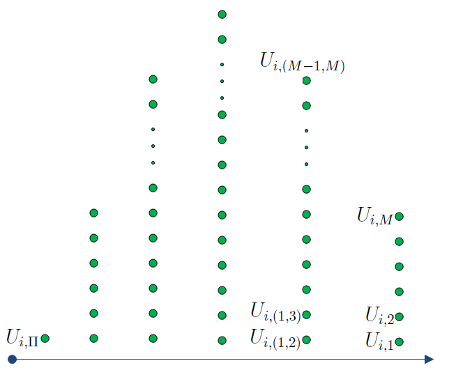
Figure 7: Illustrates the order of codebook generation at source $i$

Encoding : Suppose we are given $\{U_{\Sigma}\}{}_{2^{\Pi}-\phi}$ satisfying (30). As in section III-C, the encoding at each node is divided into 3 stages:

1) Stage 1 : We focus on the encoding at source node $E_{i}$. The codebook generation is done following the order of $U_{i,\mathcal{K}},\,\,|\mathcal{K}|=M,M-1,M-2\ldots,1$ as shown in Fig. 7. First, $2^{nR_{i,\Pi}^{{}^{\prime}}}$ independent codewords of $U_{i,\Pi}$, $u_{i,\Pi}^{n}(j)\,\,j\in\{1\ldots 2^{nR_{i,\Pi}^{{}^{\prime}}}\}$, are generated according to the density $\prod_{t=1}^{n}P_{U_{i,\Pi}}(u_{i,\Pi}^{(t)})$. Conditioned on each codeword $u_{i,\Pi}^{n}(j)$, $2^{nR_{i,\mathcal{K}}^{{}^{\prime}}}$ codewords of $U_{i,\mathcal{K}}:|\mathcal{K}|=M-1$ are generated independent of each other according to the conditional density $\prod_{t=1}^{n}P_{U_{i,\mathcal{K}}|U_{i,\Pi}}(u_{i,\mathcal{K}}^{(t)}|u_{i,\Pi}^{(t)})$. Similarly, $\forall\mathcal{K}:|\mathcal{K}|<M$, $2^{nR_{i,\mathcal{K}}^{{}^{\prime}}}$ codewords of $U_{i,\mathcal{K}}$ are independently generated conditioned on each codeword tuple of $\{U_{i}\}_{\mathcal{I}_{|\mathcal{K}|+}(\mathcal{K})}$ according to $\prod_{t=1}^{n}P_{U_{i,\mathcal{K}}|\{U_{i}\}_{\mathcal{I}_{|\mathcal{K}|+}(\mathcal{K})}}(u_{i,\mathcal{K}}^{(t)}|\{u_{i}\}_{\mathcal{I}_{|\mathcal{K}|+}(\mathcal{K})}^{(t)})$. Note that to generate the codewords of $U_{i,\mathcal{K}}$, we first need all the codebooks of $\{U_{i}\}_{\mathcal{I}_{|\mathcal{K}|+}(\mathcal{K})}$. On observing a sequence, $x_{i}^{n}$, the encoder at $E_{i}$ attempts to find a set of codewords, one for each variable, such that they are all jointly typical. If it fails to find such a set, it declares an error. Codebooks are generated similarly at all the source nodes. Note that all the random variables $U_{i,i}\forall i\in\Sigma$ can be set to constants without changing the rate region of Theorem 1. However, we continue to use them to avoid more complex notation.

2) Stage 2 : In stage 2, the codewords in each codebook are divided into uniform bins. Specifically, the $2^{nR_{i,\mathcal{K}}^{{}^{\prime}}}$ codewords in any codebook of $U_{i,\mathcal{K}}$ are subdivided into $2^{nR_{i,\mathcal{K}}^{{}^{\prime\prime}}}$ bins, with each bin containing $2^{n(R_{i,\mathcal{K}}^{{}^{\prime}}-R_{i,\mathcal{K}}^{{}^{\prime\prime}})}$ codewords. All the codewords which have the same bin index $m$ are said to fall in the bin $\mathcal{C}_{i,\mathcal{K}}(m)$ $\forall m\in(1\ldots 2^{nR_{i,\mathcal{K}}^{{}^{\prime\prime}}})$. If in stage 1, the encoder succeeds in finding a jointly typical set of codewords, the bin index of the codeword of $U_{i,\mathcal{K}}$ is sent as part of packet $\mathcal{P}_{i,\mathcal{K}}$.

3) Stage 3 : Power Binning : In this stage, each typical sequence of $X_{i}$ is assigned $2^{|\Pi_{i}|}-1$ indices, randomly generated using uniform pmfs over $(1,\ldots,2^{\tilde{R}_{i,\mathcal{K}}})\,\,\forall\mathcal{K}\in 2^{\Pi_{i}}-\phi$, respectively. All the sequences of $i$ which have the same bin index $l$ are said to fall in the bin $\mathcal{B}_{i,\mathcal{K}}(l)$ $\forall l\in(1\ldots 2^{n\tilde{R}_{i,\mathcal{K}}})$. On observing a sequence $x_{i}^{n}$, if it is typical, the encoder sends the corresponding bin indices in the packets $\mathcal{P}_{i,\mathcal{K}}:\mathcal{K}\in 2^{\Pi_{i}}-\phi$, in addition to the bin indices in stage 2. If it is not typical, the encoder declares an error. Note that all packets from source node $E_{i}$ to a subset of sinks $\mathcal{K}$ such that $\mathcal{K}\subseteq 2^{\Pi_{i}}-\phi$, carry two bin indices, one each from stages 2 and 3, respectively.

In Appendix Appendix A: Bounding Encoding/Decoding Errors in Theorem 1, we show that, if the rates $R_{i,\mathcal{K}}^{{}^{\prime}}$ satisfy (34), then the probability of encoding error asymptotically approaches zero, i.e., we can, with probability approaching 1, find a codeword tuple, one from each codebook such that all the codewords are jointly typical if the rates satisfy (34). Let the codewords, which are jointly typical with $x_{i}^{n}$, be denoted as $u_{i,\mathcal{K}}^{*}$ $\forall\mathcal{K}\in\mathcal{J}(\Pi)=2^{\Pi}-\phi$. To ensure joint typicality of $(\{x\}_{\Sigma}^{n},\{u_{\Sigma}^{*}\}_{\mathcal{J}(k)})$, we require a stronger version of the “conditional Markov lemma” in [10]. We state and prove this stronger version, called the “conditional Markov lemma for mutual covering” in Appendix B. From this lemma, it follows that $\left(\{x\}_{\Sigma}^{n},\{u_{\Sigma}^{*}\}_{\mathcal{J}(k)}\right)\in\mathcal{T}_{\epsilon}^{n}\left(\{X\}_{\Sigma}^{n},\{U_{\Sigma}^{*}\}_{\mathcal{J}(k)}\right)$ with very high probability given that the encoding at all the source nodes is error free. Let the bin indices of $u_{i,\mathcal{K}}^{*}$ (assigned in stage 2) be denoted by $m_{i,\mathcal{K}}\,\,\forall\mathcal{K}\in 2^{\Pi}-\phi$ and let the bin indices of $x_{i}^{n}$ (assigned in stage 3) be denoted by $l_{i,\mathcal{K}}\forall\mathcal{K}\in 2^{\Pi_{i}}-\phi$.

Decoding : We focus on a particular sink $S_{k}$. Sink $S_{k}$ receives all the indices $\{m_{\Sigma}\}_{\mathcal{J}(k)}$ of stage 2 of encoding from all source nodes. It also receives $\{l_{\Sigma_{k}}\}_{\mathcal{J}(k)}$ of stage 3 of encoding from source nodes $\Sigma_{k}$. In the first stage of decoding, it begins decoding $u_{i,\mathcal{J}(k)}^{*}\,\,\forall i\in\Sigma$ by looking for a unique jointly typical codeword tuple from $\{\mathcal{C}_{i,\mathcal{J}(k)}(m_{i,\mathcal{J}(k)});\forall i\in\Sigma\}$. Clearly $\{u_{\Sigma}^{*}\}_{\mathcal{J}(k)}$ satisfies this property. If the decoder finds another such jointly typical codeword tuple in the received bins, it declares an error. In Appendix Appendix A: Bounding Encoding/Decoding Errors in Theorem 1, we show that if conditions (35) are satisfied by $R_{i,\mathcal{K}}^{{}^{\prime\prime}}$, then the probability that the decoder finds another such jointly typical codeword tuple approaches zero.

In the last stage of decoding, after having decoded all $\{u_{\Sigma}^{*}\}_{\mathcal{J}(k)}$, the decoder looks for unique source sequences from $\bigcap\{\mathcal{B}_{i,\mathcal{K}}(l_{i,\mathcal{K}}):i\in\Sigma_{k},\mathcal{K}\ni k\}$ which are jointly typical with $\{u_{\Sigma}^{*}\}_{\mathcal{J}(k)}$. Hence what remains is to find conditions on $\tilde{R}_{i,\mathcal{K}}$ to ensure lossless reconstruction of the respective sources at each sink. Following similar steps as in [3, 4], it is easy to show that this probability can be made arbitrarily small if (36) is satisfied $\forall\Gamma\in 2^{\Sigma_{k}}-\phi$. We have shown that if the rates satisfy the conditions in Theorem 1, the probability of decoding error at each sink can be made arbitrarily small. Arbitrarily small decoding error ensures that the decoder decodes the correct sequence with very high probability. Hence, if the rate constraints are satisfied, for any $\epsilon>0$, we can find a sufficiently large $n$ such that:

$$P(\hat{X}_{\sum_{j}}^{n}\neq X_{\sum_{j}}^{n})<\epsilon$$ (38)

Recall that packets from source node $E_{i}$ to sinks $\mathcal{K}\subseteq\Pi_{i}$ carry both $m_{i,\mathcal{K}}$ (at rate $R_{i,\mathcal{K}}^{{}^{\prime\prime}}$) and $l_{i,\mathcal{K}}$ (at rate $\tilde{R}_{i,\mathcal{K}}$). While the other packets carry only $m_{i,\mathcal{K}}$ (at rate $R_{i,\mathcal{K}}^{{}^{\prime\prime}}$). Hence, the rates of each packet must satisfy the following constraints for lossless decoding of the requested sources:

$$R_{i,\mathcal{K}}\geq\begin{cases}R_{i,\mathcal{K}}^{{}^{\prime\prime}}+\tilde{R}_{i,\mathcal{K}}&\mbox{if }\mathcal{K}\subseteq 2^{\Pi_{i}}-\phi\\ R_{i,\mathcal{K}}^{{}^{\prime\prime}}&\mbox{if }\mathcal{K}\nsubseteq 2^{\Pi_{i}}-\phi\end{cases}$$ (39)

proving the theorem.∎

Remark 3.

A note on separability of distributed compression and routing : It was shown in [1] that the two problems of DSC (Slepian-Wolf compression) and optimum broadcast routing are separable problems, i.e., the optimum routes can be found without the knowledge of the achievable rates, and vice versa, the rate region can be found without the knowledge of the routes. However, we demonstrated in [21] that such separability holds only under the ‘no helpers’ assumption. We also showed that the extent of suboptimality due to separating DSC and broadcast routing is substantial and potentially unbounded when helpers are allowed to communicate. In general the optimum rate region cannot be found without the knowledge of the network costs for broadcast routing. However, for DIR, the two problems of finding the optimum rate region for the tuple $(R_{i,\mathcal{K}}\,\,\forall i\in\Sigma,\mathcal{K}\in 2^{\Pi}-\phi)$ and finding the optimum routes from the source nodes to the sinks can be separated and dealt independently, without entailing any loss of optimality. Note that even though DIR has the inherent advantage of separability, finding the optimum operating point requires optimizing over an $N\times 2^{M}$ dimensional space and the effective complexity remains the same as that for broadcast routing.

V Outerbounds to certain special scenarios

We note that the converse to the achievability region does not hold in general. However, we can prove the converse for two important special cases.

V-A When there are no helpers

Theorem 2.

When each sink is allowed to receive packets only from sources it intends to reconstruct, the complete rate region for dispersive information routing is given by: $\forall j\in\Pi$ and $\forall\mathcal{S}\in 2^{\Sigma_{j}}-\phi$:

$$\sum_{i\in\mathcal{S}}\sum_{\mathcal{K}\in 2^{\Pi_{i}}-\phi,\,\,\mathcal{K}\ni j}R_{i,\mathcal{K}}\geq H\left(\{X\}_{\mathcal{S}}|\{X\}_{\Sigma_{j}-\mathcal{S}}\right)$$ (40)

It is achieved by ‘Power Binning’.

Proof.

In the achievable rate region of Theorem 1, setting $U_{i,\mathcal{S}}=\Phi\,\,\forall i\in\Sigma,\mathcal{S}\in 2^{\Pi}-\phi$, where $\Phi$ is a constant, leads to the above rate region. The converse to this rate region follows directly from the converse to the lossless source coding theorem [26]. We omit the proof as it is straightforward. ∎

V-B A 2-Sink network with a single helper

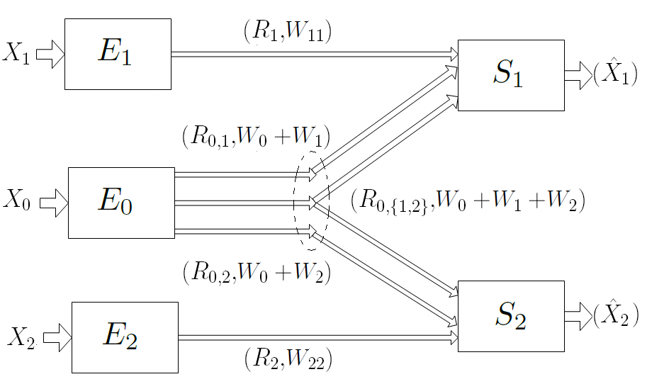
Figure 8: Example of a 2-sink, 1 Helper DIR

The converse can be proven in general for any 2 sink network with a single helper. However, to avoid complex notation, we just give a simple example of a 2 sink network with a single helper and prove the converse to the rate region. The proof of converse for a general 2 sink network with a single helper follows in similar lines.

Consider the network shown in Fig. 8, with 3 source nodes and 2 sinks. The three source nodes $E_{1},E_{0},E_{2}$ observe three correlated memoryless random sequences $X_{1}^{n},X_{0}^{n},X_{2}^{n}$, respectively. The two sinks $S_{1}$ and $S_{2}$ respectively reconstruct $X_{1}^{n}$ and $X_{2}^{n}$ losslessly. Note that $E_{0}$ acts as a helper to both the sinks. Our objective is to find the rate region for the tuple $(R_{1},R_{2},R_{0,1},R_{0,2},R_{0,\{1,2\}})$ for lossless reconstruction of the respective sources. It is important to remember that our ultimate objective is to find the minimum communication cost, which follows by finding the point in the rate region that minimizes the following cost function:

$$C_{DIR}^{*}=W_{11}R_{1}+W_{22}R_{2}+(W_{0}+W_{1})R_{0,1}$$

$$+(W_{0}+W_{2})R_{0,2}+(W_{0}+W_{1}+W_{2})R_{0,\{1,2\}}$$ (41)

The following theorem establishes the complete rate region.

Theorem 3.

Let $(U_{0},U_{1},U_{2})$ be random variables distributed over arbitrary finite sets $\mathcal{U}_{0}\times\mathcal{U}_{1}\times\mathcal{U}_{2}$, jointly distributed with $(X_{1},X_{0},X_{2})$ such that the following hold:

$$X_{1} \leftrightarrow X_{0}\leftrightarrow(U_{0},U_{1},U_{2})$$

$$X_{2} \leftrightarrow X_{0}\leftrightarrow(U_{0},U_{1},U_{2})$$ (42)

Then any rate tuple satisfying the following constraints is achievable for the 2-Sink 1-Helper DIR problem:

$$R_{0,12} \geq I(X_{0};U_{0})$$

$$R_{0,1} \geq I(X_{0};U_{1}|U_{0})$$

$$R_{0,2} \geq I(X_{0};U_{2}|U_{0})$$

$$R_{1,1} \geq H(X_{1}|U_{0},U_{1})$$

$$R_{2,2} \geq H(X_{2}|U_{0},U_{2})$$ (43)

The closure of the achievable rates over all such $(U_{0},U_{1},U_{2})$ is the complete rate region for this setup.

Proof.

Achievability : Let $(U_{0},U_{1},U_{2})$ be any random variables satisfying (42). The following achievable rate region is obtained by setting $U_{0,12}=U_{0}$, $U_{0,1}=U_{1}$, $U_{0,12}=U_{2}$ and all the remaining random variables to constants in the general achievable rate region of Theorem 1:

$$R_{0,12} \geq I(X_{0};U_{0})$$

$$R_{0,12}+R_{0,1} \geq I(X_{0};U_{0})+I(X_{0};U_{1}|U_{0})$$

$$R_{0,12}+R_{0,2} \geq I(X_{0};U_{0})+I(X_{0};U_{2}|U_{0})$$

$$R_{0,12}+R_{0,1}+R_{0,2} \geq I(X_{0};U_{1},U_{2},U_{0})+I(U_{1};U_{2}|U_{0})$$

$$R_{1,1} \geq H(X_{1}|U_{0},U_{1})$$

$$R_{2,2} \geq H(X_{2}|U_{0},U_{2})$$ (44)

We further restrict the joint density to satisfy the following Markov condition in addition to (42):

$$U_{1}\leftrightarrow(X_{0},U_{0})\leftrightarrow U_{2}$$ (45)

On using this Markov condition in (44), the sum rate constraint on $R_{0,12}+R_{0,1}+R_{0,2}$ becomes:

$$R_{0,12}+R_{0,1}+R_{0,2}\geq I(X_{0};U_{0})+I(X_{0};U_{1}|U_{0})$$

$$+I(X_{0};U_{2}|U_{0})$$ (46)

Observe that if a rate tuple satisfies (43), then it also satisfies (44) and hence the region given by (43) is achievable for the 2-Sink 1-Helper problem shown in Fig. 8.

Converse : Recall the notation in the definition of an achievable rate region in Section IV-B. The output of encoder 1 is denoted $f_{1}^{E}(X_{1}^{n})=T_{1}$ and the output of encoder 2 is $f_{2}^{E}(X_{2}^{n})=T_{2}$. Remember that $0\leq T_{1}\leq 2^{nR_{1}}$ and $0\leq T_{1}\leq 2^{nR_{2}}$. Similarly the encoder at $E_{0}$ transmits 3 indices denoted by $(T_{0,1},T_{0,2},T_{0,12})$ which are routed to the respective sinks. Sink $S_{1}$ receives $(T_{1},T_{0,1},T_{0,12})$ and reconstructs $X_{1}^{n}$ with vanishing probability of error. Similarly sink $S_{2}$ receives $(T_{2},T_{0,2},T_{0,12})$ and reconstructs $X_{2}^{n}$ losslessly. We need to prove that for any code with vanishing probability of error, the rates must satisfy (43) for some $(U_{0},U_{1},U_{2})$ satisfying (42).

We follow standard converse techniques to prove the above claim. We begin with the following series of inequalities:

$$nR_{0,12} \geq H(T_{0,12})\geq I(X_{0}^{n};T_{0,12})$$ (47)

$$= \sum_{i=1}^{n}I(X_{0}^{i};T_{0,12}|X_{0}^{1,i-1})$$

$$=^{(a)} \sum_{i=1}^{n}I(X_{0}^{i};T_{0,12},X_{0}^{1,i-1})$$

$$=^{(b)} \sum_{i=1}^{n}I(X_{0}^{i};U_{0,12}^{i})$$

where $(a)$ follows from the memoryless property of the sources and $(b)$ follows by setting $U_{0,12}^{i}=(T_{0,12},X_{0}^{1,i-1})$. Here $X_{0}^{i}$ denotes the $i$’th realization of $X_{0}^{n}$ and $X_{0}^{1,i-1}$ denotes the first $i-1$ realizations of $X_{0}^{n}$. Next we have:

$$nR_{0,1} \geq H(T_{0,1})\geq H(T_{0,1}|T_{0,12})$$ (48)

$$\geq I(X_{0}^{n};T_{0,1}|T_{0,12})$$

$$= \sum_{i=1}^{n}I(X_{0}^{i};T_{0,1}|T_{0,12},X_{0}^{1,i-1})$$

$$= \sum_{i=1}^{n}I(X_{0}^{i};U_{0,1}^{i}|U_{0,12}^{i})$$

Where $U_{0,1}^{i}=(T_{0,1})\,\,\forall i$. Similarly, we can show that:

$$nR_{0,2}\geq\sum_{i=1}^{n}I(X_{0}^{i};U_{0,2}^{i}|U_{0,12}^{i})$$ (49)

where $U_{0,2}^{i}=(T_{0,2})\,\,\forall i$. Note that as $(T_{0,1},T_{0,2},T_{0,12},X_{0}^{1,i-1})$ depends on $(X_{1}^{i},X_{2}^{i})$ only through $X_{0}^{i}$, we have the following two Markov chain conditions:

$$X_{1}^{i} \leftrightarrow X_{0}^{i}\leftrightarrow(U_{0}^{i},U_{1}^{i},U_{2}^{i})$$

$$X_{2}^{i} \leftrightarrow X_{0}^{i}\leftrightarrow(U_{0}^{i},U_{1}^{i},U_{2}^{i})$$ (50)

Further, we need lossless reconstruction of $X_{1}^{n}$ at $S_{1}$. The following series of inequalities hold:

$$nR_{1} \geq H(T_{1})$$ (51)

$$\geq H(T_{1}|T_{0,12},T_{0,1})$$

$$= H(T_{1}|T_{0,12},T_{0,1})+H(X_{1}^{n}|T_{0,12},T_{0,1},T_{1})$$

$$-H(X_{1}^{n}|T_{0,12},T_{0,1},T_{1})$$

$$\geq^{(a)} H(X_{1}^{n},T_{1}|T_{0,12},T_{0,1})-n\epsilon_{n}$$

$$= H(X_{1}^{n}|T_{0,12},T_{0,1})-n\epsilon_{n}$$

$$= \sum_{i=1}^{n}H(X_{1}^{i}|X_{1}^{i-1},T_{0,12},T_{0,1})-n\epsilon_{n}$$

$$= \sum_{i=1}^{n}H(X_{1}^{i}|U_{0,12}^{i},U_{0,1}^{i})-n\epsilon_{n}$$

where $(a)$ follows from Fano’s inequality, i.e., $H(X_{1}^{n}|T_{1},T_{0,1},T_{0,12})<n\epsilon_{n}$. Similarly, for lossless reconstruction at $S_{2}$, we have:

$$nR_{2}\geq\sum_{i=1}^{n}H(X_{2}^{i}|U_{0,12}^{i},U_{0,2}^{i})-n\epsilon_{n}$$ (52)

We next introduce a time sharing random variable $Q\sim\mbox{Unif}[1:n]$, independent of $(X_{0}^{n},X_{1}^{n},X_{2}^{n},U_{0,1}^{n},U_{0,2}^{n},U_{0,12}^{n})$, so that we can rewrite (47), (48), (49), (51) and (52) as:

$$nR_{0,12} \geq I(X_{0}^{Q};U_{0,12}^{Q}|Q)=I(X_{0}^{Q};U_{0,12}^{Q},Q)$$

$$nR_{0,1} \geq I(X_{0}^{Q};U_{0,1}^{Q}|U_{0,12}^{Q},Q)$$

$$= I(X_{0}^{Q};U_{0,1}^{Q},Q|U_{0,12}^{Q},Q)$$

$$nR_{0,2} \geq I(X_{0}^{Q};U_{0,2}^{Q}|U_{0,12}^{Q},Q)$$

$$= I(X_{0}^{Q};U_{0,2}^{Q},Q|U_{0,12}^{Q},Q)$$

$$nR_{1} \geq H(X_{1}^{Q}|U_{0,12}^{Q},U_{0,1}^{Q},Q)$$

$$nR_{2} \geq H(X_{2}^{Q}|U_{0,12}^{Q},U_{0,2}^{Q},Q)$$ (53)

Setting $(U_{0,12}^{Q},Q)=U_{0,12}$, $(U_{0,1}^{Q},Q)=U_{0,1}$, $(U_{0,2}^{Q},Q)=U_{0,2}$ and observing that $(X_{0}^{Q},X_{1}^{Q},X_{2}^{Q})$ has the same density as $(X_{0},X_{1},X_{2})$ we get the rate region given in (43). ∎

Example to demonstrate strict improvement: Next we show that DIR achieves strictly lower communication cost for the single helper network shown in Fig. 8. This example demonstrates the freedom DIR provides over broadcast routing by sending only the relevant information to each sink, even when the information is from a helper. The complete rate region under broadcast routing for the example shown in Fig. 8 was determined in [14, 33] and is given by the closure of the following rate tuples over all random variables $U_{0}$ satisfying $(X_{1},X_{2})\leftrightarrow X_{0}\leftrightarrow U_{0}$:

$$R_{0,12} \geq I(X_{0};U_{0})$$

$$R_{1,1} \geq H(X_{1}|U_{0})$$

$$R_{2,2} \geq H(X_{2}|U_{0})$$ (54)

We consider the example where $(X_{0},X_{1},X_{2})$ are binary symmetric sources such that $X_{1}\leftrightarrow X_{0}\leftrightarrow X_{2}$ holds. The transition probabilities are such that $X_{1}$ and $X_{2}$ are obtained as outputs of two independent binary symmetric channels with $X_{0}$ as input and cross-over probabilities of $P_{1}$ and $P_{2}$, respectively. Let us say that the network costs are such that $E_{1}$ and $E_{2}$ send at rates $\Delta$ more than their respective conditional entropies (for some $\Delta>0$), i.e., $R_{1}=H_{b}(P_{1})+\Delta$ and $R_{2}=H_{b}(P_{2})+\Delta$ where $H_{b}(\cdot)$ denotes the binary entropy function (note that the conditional entropy is the minimum information each encoder has to send). Wyner [14] (see also [34]) showed that the minimum rate from $E_{0}$ to the two sinks under broadcast routing is given by:

$$R_{0} \geq\max_{P_{0}\in\{P_{01},P_{02}\}}1-H_{b}(P_{0})$$ (55)

where $P_{01}$ and $P_{02}$ solve the respective equations $H_{b}(P_{1}\bullet P_{01})=H_{b}(P_{1})+\Delta$ and $H_{b}(P_{2}\bullet P_{02})=H_{b}(P_{2})+\Delta$ where $P_{1}\bullet P_{2}=P_{1}P_{2}+(1-P_{1})(1-P_{2})$. The optimum $U_{0}$ which achieves the boundary points is obtained by passing $X_{0}$ through a binary symmetric channel (BSC) with cross over probability $P_{0}$. Again observe that, if the sinks $S_{1}$ and $S_{2}$ receive information from $E_{1}$ and $E_{2}$ at rates $H_{b}(P_{1})+\Delta$ and $H_{b}(P_{2})+\Delta$, they require information from $E_{0}$ at rates $1-H_{b}(P_{01})$ and $1-H_{b}(P_{02})$, respectively. However, broadcast routing sends information at the maximum of the two to both sinks and hence if $P_{1}\neq P_{2}$ (which in turn implies $P_{01}\neq P_{02}$ in general), there is sub-optimality on either one of the two branches connecting from the collector to the two sinks.

On the other hand, using DIR, we can achieve minimum rates on all the branches. To prove this claim, without loss of generality, let us assume that $0.5>P_{01}>P_{02}>0$. Consider the following joint density for $(U_{0},U_{1},U_{2})$ in Theorem 3. $U_{2}$ is the output when $X_{0}$ is sent through a BSC with cross over probability $P_{02}$ and $U_{0}$ is the output when $U_{2}$ is sent through a BSC with cross over probability $P_{012}$ where $P_{02}\bullet P_{012}=P_{01}$. $U_{1}$ is set as a constant. It is easy to verify from Theorem 3 that the following rates are achievable:

$$R_{0,12} =1-H_{b}(P_{01})$$

$$R_{0,2} =H_{b}(P_{01})-H_{b}(P_{02})$$ (56)

which implies that the two sinks receive at their respective minima leading to the conclusion that DIR achieves the minimum communication cost for this example.

VI Conclusion

This paper considers a new routing paradigm called dispersive information routing, wherein each intermediate node is allowed to “split a packet” and forward subsets of the information on individual forward paths. We demonstrated using simple examples the gains of DIR over broadcast routing. Unlike network coding, this new routing technique can be realized using conventional routers with source nodes transmitting multiple smaller packets into the network. This paradigm introduces a new class of information theoretic problems. We derived an achievable rate region for this setup using principles from multiple descriptions encoding and Han and Kobayashi decoding which is complete for certain special cases of the setup.

Appendix A: Bounding Encoding/Decoding Errors in Theorem 1

Proof.

Probability of encoding error : Let us analyze the probability of encoding error at source node $E_{i}$. Let $\mathcal{E}$ denote the event of an encoding error. We have:

$$P(\mathcal{E}) = P(\mathcal{E}|x_{i}^{n}\in\mathcal{T}_{\epsilon}^{n})P(x_{i}^{n}\in\mathcal{T}_{\epsilon}^{n})$$ (57)

$$+P(\mathcal{E}|x_{i}^{n}\notin\mathcal{T}_{\epsilon}^{n})P(x_{i}^{n}\notin\mathcal{T}_{\epsilon}^{n})$$

From standard typicality arguments, we have $P(x_{i}^{n}\notin\mathcal{T}_{\epsilon}^{n})\rightarrow 0$ as $n\rightarrow\infty$. Hence, it is sufficient to find conditions on the rates to bound $P(\mathcal{E}|x_{i}^{n}\in\mathcal{T}_{\epsilon}^{n})$.

Towards finding conditions on the rate to bound $P(\mathcal{E}|x_{i}^{n}\in\mathcal{T}_{\epsilon}^{n})$, we define the random variables :

$$\chi(\{j\}_{\mathcal{J}(\Pi)})=\begin{cases}1&\mbox{if}\,\,\left(x_{i}^{n},u_{i}^{n}(\{j\}_{\mathcal{J}(\Pi)})\right)\in\mathcal{T}_{\epsilon}^{n}\\ 0&\mbox{else}\end{cases}$$ (58)

We have $P(\mathcal{E}|x_{i}^{n}\in\mathcal{T}_{\epsilon}^{n})=P(\Psi=0)$ where $\Psi=\sum_{\mathcal{J}(\Pi)}\chi(\{j\}_{\mathcal{J}(\Pi)})$. From Chebyshev’s inequality, it follows that:

$$P(\Psi=0)\leq P\left[|\Psi-E[\Psi]|\geq E[\Psi]/2\right]\leq\frac{4\mbox{Var}(\Psi)}{\left(E[\Psi]\right)^{2}}$$ (59)

From Lemma 3.1 in [3], we can bound $E[\Psi]$ as follows:

$$E[\Psi]\geq 2^{n\sum_{\mathcal{K}\in\mathcal{J}(\Pi)}R_{\mathcal{K}}^{{}^{\prime}}-n\left(\alpha(i,\mathcal{J}(\Pi))+\epsilon\right)}$$ (60)

where

$$\alpha(i,\mathcal{Q}) = -H\left(\{U_{i}\}_{\mathcal{Q}}|X_{i}\right)$$ (61)

$$+\sum_{\mathcal{K}\in\mathcal{Q}}H\left(U_{i,\mathcal{K}}|\{U_{i}\}_{\mathcal{I}_{|\mathcal{K}|+}(\mathcal{K})}\right)$$

$\forall i,\mathcal{Q}\subseteq\mathcal{J}(\Pi)$. We follow the convention $\alpha_{W}(i,\phi)=0$. Next consider $\mbox{Var}(\Psi)=E[\Psi^{2}]-\left(E[\Psi]\right)^{2}$ where,

$$E[\Psi^{2}]=\sum_{\{j\}_{\mathcal{J}(\Pi)}}\sum_{\{k\}_{\mathcal{J}(\Pi)}}E\left[\chi(\{j\}_{\mathcal{J}(\Pi)})\chi(\{k\}_{\mathcal{J}(\Pi)})\right]$$

$$=\sum_{\{j\}_{\mathcal{J}(\Pi)}}\sum_{\{k\}_{\mathcal{J}(\Pi)}}P\left[\chi(\{j\}_{\mathcal{J}(\Pi)})=1,\chi(\{k\}_{\mathcal{J}(\Pi)})=1\right]$$ (62)

The probability in (62) depends on whether $u_{i}^{n}(\{j\}_{\mathcal{J}(\Pi)})$ and $u_{i}^{n}(\{k\}_{\mathcal{J}(\Pi)})$ are equal for a subset of indices. Let $\mathcal{Q}\subseteq\mathcal{J}(\Pi),\,\,\mathcal{Q}\neq\phi$, such that $\{j\}_{\mathcal{Q}}=\{k\}_{\mathcal{Q}}$. Observe that, due to the hierarchical structure in the conditional codebook generation mechanism, for $u_{i}^{n}(\{j\}_{\mathcal{Q}})=u_{i}^{n}(\{k\}_{\mathcal{Q}})$ to hold, $\mathcal{Q}$ must be such that,

$$\mbox{if }\mathcal{K}\in\mathcal{Q}\,\,\Rightarrow\,\,\,\mathcal{I}_{|\mathcal{K}|+}(\mathcal{K})\subset\mathcal{Q}$$ (63)

i.e., $\mathcal{Q}\in\mathcal{Q}^{*}$ given in (29). It follows from the codebook generation mechanism that given the codeword tuple $\{u_{i}^{n}(\{j\}_{\mathcal{Q}})\}$, tuples $\{u_{i}^{n}(\{j\}_{\mathcal{J}(\Pi)-\mathcal{Q}})\}$ and $\{u_{i}^{n}(\{k\}_{\mathcal{J}(\Pi)-\mathcal{Q}})\}$ are independent and identically distributed. Hence we can rewrite the probability in (62) for some $\mathcal{Q}\subseteq\mathcal{J}(\Pi),\,\,\mathcal{Q}\neq\phi$, as:

$$P\left[\mathcal{E}(\{j\}_{\mathcal{J}(\Pi)})\cap\mathcal{E}(\{k\}_{\mathcal{J}(\Pi)})\right]=\left(\frac{P\left[\mathcal{E}(\{j\}_{\mathcal{J}(\Pi)})\right]}{P\left[\mathcal{E}(\{j\}_{\mathcal{Q}})\right]}\right)^{2}$$

$$\times P\left[\mathcal{E}(\{j\}_{\mathcal{Q}})\right]$$ (64)

However, note that if $\mathcal{Q}=\phi$, then:

$$P\left[\mathcal{E}(\{j\}_{\mathcal{J}(\Pi)})\cap\mathcal{E}(\{k\}_{\mathcal{J}(\Pi)})\right]=\left(P\left[\mathcal{E}(\{j\}_{\mathcal{J}(\Pi)})\right]\right)^{2}$$ (65)

Next, the total number of ways of choosing $\{j\}_{\mathcal{J}(\Pi)}$ and $\{k\}_{\mathcal{J}(\Pi)}$ such that they overlap in the subset $\mathcal{Q}$ is:

$$2^{n\sum_{\mathcal{K}\in\mathcal{Q}}R_{i,\mathcal{K}}^{{}^{\prime}}}\prod_{\mathcal{K}\in\mathcal{J}(\Pi)-\mathcal{Q}}2^{nR_{i,\mathcal{K}}^{{}^{\prime}}}(2^{nR_{i,\mathcal{K}}^{{}^{\prime}}}-1)$$

$$\leq 2^{n\{\sum_{\mathcal{K}\in\mathcal{J}(\Pi)}R_{i,\mathcal{K}}^{{}^{\prime}}+2\sum_{\mathcal{K}\in\mathcal{J}(\Pi)-\mathcal{Q}}R_{i,\mathcal{K}}^{{}^{\prime}}\}}$$ (66)

On substituting (64) and (66) in (62), we bound $\mbox{Var}(\Psi)$ as:

$$\mbox{Var}(\Psi) \leq \sum\biggl{\{}2^{-2n\left(\alpha(i,\mathcal{J}(\Pi))-\sum_{\mathcal{K}\in\mathcal{J}(\Pi)}R_{i,\mathcal{K}}^{{}^{\prime}}\right)}$$ (67)

$$2^{n\left(\alpha(i,\mathcal{Q})-\sum_{\mathcal{K}\in\mathcal{Q}}R_{i,\mathcal{K}}^{{}^{\prime}}\right)+5n\epsilon}\biggl{\}}$$

where the summation is over all non-empty $\mathcal{Q}$ such that (63) holds. Observe that the term corresponding to $\mathcal{Q}=\phi$ gets canceled with the ‘$(\mathcal{E}[\Psi])^{2}$’ term in $\mbox{Var}(\Psi)$. Inserting, (67) and (60) in (59), we get :

$$P(E|x_{i}^{n}\in\mathcal{T}_{\epsilon}^{n})\leq 4\sum 2^{n\left(\alpha(i,\mathcal{Q})-\sum_{\mathcal{K}\in\mathcal{Q}}R_{\mathcal{K}}^{{}^{\prime}}\right)+7n\epsilon}$$ (68)

where the summation is over all non-empty $\mathcal{Q}$ satisfying (63). Hence, the probability of encoding error at all the source nodes can be made arbitrarily small if:

$$\sum_{\mathcal{K}\in\mathcal{Q}}R_{i,\mathcal{K}}^{{}^{\prime}}\geq\alpha(i,\mathcal{Q})+7\epsilon$$ (69)

$\forall i,\mathcal{Q}$ satisfying (63).

Probability of decoding error : We focus on decoding at sink $S_{k}$. We first bound the probability of error for the first stage of decoding. The decoder looks for a unique codeword tuple from $\Bigl{\{}\{\mathcal{C}_{\Sigma}\}_{\mathcal{J}(k)}\bigl{(}\{m_{\Sigma}\}_{\mathcal{J}(k)}\bigr{)}\Bigr{\}}$ which are jointly typical. We know that $\{u_{\Sigma}^{*}\}_{\mathcal{J}(k)}$ are jointly typical from the Markov Lemma in Appendix B. We have to find conditions on $R_{i,\mathcal{S}}^{{}^{\prime\prime}}$ to ensure no other tuple satisfies this property. Denote by $\mathcal{F}$ the event of a decoding error given the encoding is error-free. Due to the symmetry in codebook generation, we can assume that the index tuple of $\{u_{\Sigma}^{*}\}_{\mathcal{J}(k)}$ is $(1,\ldots,1)$. Let $\{j_{\Sigma}\}_{\mathcal{J}(k)}$ be an index tuple such that:

$$\{j_{\Sigma}\}_{\mathcal{J}(k)}\neq(1,\ldots,1)$$ (70)

Define the event $\mathcal{F}(\{j_{\Sigma}\}_{\mathcal{J}(k)})$ as:

$$\mathcal{F}(\{j_{\Sigma}\}_{\mathcal{J}(k)})=\Bigl{\{}\left(u_{\Sigma}^{n}(\{j_{\Sigma}\}_{\mathcal{J}(k)})\right)\in\mathcal{T}_{\epsilon}^{n}\Bigr{\}}$$ (71)

It then follows from union bound that:

$$P(\mathcal{F}) \leq \sum P\bigl{(}\mathcal{F}(\{j_{\Sigma}\}_{\mathcal{J}(k)})\bigr{)}$$ (72)

where the summation is over all $\{j_{\Sigma}\}_{\mathcal{J}(k)}\neq(1,\ldots,1)$. However, a subset of indices of $\{j_{\Sigma}\}_{\mathcal{J}(k)}$ can still be equal to $1$. We expand the above summation over all such possible subsets. Let $\mathcal{Q}_{1},\mathcal{Q}_{2},\ldots\mathcal{Q}_{N}\subseteq\mathcal{J}(k)$ satisfying (63) be such that the following holds:

$$\exists i\in\{1,2,\dots,N\}:\mathcal{Q}_{i}\subset\mathcal{J}(k)$$ (73)

i.e., at least one of the $\mathcal{Q}_{i}$’s is a strict subset of $\mathcal{J}(k)$. Define the set:

$$A_{\mathcal{Q}_{1},\mathcal{Q}_{2},\ldots,\mathcal{Q}_{N}}=\{j_{\Sigma}\}_{\mathcal{J}(k)}\,\,\mbox{: }\forall i\begin{cases}j_{i,\mathcal{K}}=1&\mbox{if }\mathcal{K}\in\mathcal{Q}_{i}\\ j_{i,\mathcal{K}}\neq 1&\mbox{otherwise}\end{cases}$$

Then, we can expand (72) as:

$$P(F)\leq\sum\sum P\bigl{(}\mathcal{F}(\{j_{\Sigma}\}_{\mathcal{J}(k)})\bigr{)}$$ (74)

where the first summation is over all $\{\mathcal{Q}_{1},\ldots,\mathcal{Q}_{N}:\mathcal{Q}_{i}\subseteq\mathcal{J}(k),$ satisfying (63) and (73)$\}$ and the second summation is over all $\{j_{\Sigma}\}_{\mathcal{J}(k)}\in A_{\mathcal{Q}_{1},\mathcal{Q}_{2},\ldots\mathcal{Q}_{N}}$. We note that, due to the conditional independence of the codewords generated, $P\bigl{(}\mathcal{F}(\{j_{\Sigma}\}_{\mathcal{J}(k)})\bigr{)}$ is the same for all $\{j_{\Sigma}\}_{\mathcal{J}(k)}\in A(\mathcal{Q}_{1},\mathcal{Q}_{2},\ldots\mathcal{Q}_{N})$, i.e., $P\bigl{(}\mathcal{F}(\{j_{\Sigma}\}_{\mathcal{J}(k)})\bigr{)}$ depends only on $\mathcal{Q}_{1},\mathcal{Q}_{2},\ldots\mathcal{Q}_{N}$. We can bound $P(\mathcal{F})$ as:

$$P(\mathcal{F})\leq\sum\bigl{\{}|A_{\mathcal{Q}_{1},\mathcal{Q}_{2},\ldots\mathcal{Q}_{N}}|$$

$$P\bigl{(}\mathcal{F}(\mathcal{Q}_{i};\forall i\in\Sigma)\bigr{)}\bigr{\}}$$ (75)

where $P(\mathcal{F}(\mathcal{Q}_{i};\forall i\in\Sigma))=$$P\bigl{(}\mathcal{F}(\mathcal{Q}_{1},\mathcal{Q}_{2},\ldots,\mathcal{Q}_{N})\bigr{)}$ denotes $P(\mathcal{F}(\{j_{\Sigma}\}_{\mathcal{J}(k)}))$ for some $\{j_{\Sigma}\}_{\mathcal{J}(k)}\in A_{\mathcal{Q}_{1},\mathcal{Q}_{2},\ldots\mathcal{Q}_{N}}$ and the summation is over all $\{\mathcal{Q}_{1},\ldots,\mathcal{Q}_{N}:\mathcal{Q}_{i}\subseteq\mathcal{J}(k),\mbox{ satisfying (\ref{eq:cond_Q}) and (\ref{eq:noall_1})}\}$. We next bound the individual terms in the above product. Recall that each of the bins $\mathcal{C}_{i,\mathcal{S}}(\cdot)$ have $2^{n(R_{i,\mathcal{S}}^{{}^{\prime}}-R_{i,\mathcal{S}}^{{}^{\prime\prime}})}$ codewords. Using Lemma 3.1 [3], we can bound both the terms in the above product as:

$$P\bigl{(}\mathcal{F}(\mathcal{Q}_{i};\forall i\in\Sigma)\bigr{)}\leq \frac{2^{nH\big{(}\{U_{i}\}_{\mathcal{Q}_{i}^{c}}\forall i\big{|}\{U_{i}\}_{\mathcal{Q}_{i}}\forall i\big{)}}}{2^{n\sum\limits_{i\in\Sigma}\sum\limits_{\mathcal{K}\in\mathcal{Q}_{i}^{c}}H\big{(}U_{i,\mathcal{K}}\big{|}\{U_{i}\}_{\mathcal{I}_{|\mathcal{K}|+}(\mathcal{K})}\big{)}-4n\epsilon}}$$

$$|A_{\mathcal{Q}_{1},\mathcal{Q}_{2},\ldots\mathcal{Q}_{N}}|\leq 2^{n\sum\limits_{i\in\Sigma}\sum\limits_{\mathcal{K}\in\mathcal{Q}_{i}^{c}}(R_{i,\mathcal{K}}^{{}^{\prime}}-R_{i,\mathcal{K}}^{{}^{\prime\prime}})}$$ (76)

where $\mathcal{Q}_{i}^{c}=\mathcal{J}(k)-\mathcal{Q}_{i}$. Substituting (76) in (75), it follows that $P(\mathcal{F})$ can be made arbitrarily small if: $\forall\mathcal{Q}_{1},\mathcal{Q}_{2},\ldots\mathcal{Q}_{N}\subseteq\mathcal{J}(k)$ satisfying (63) and (73),

$$\sum_{i\in\Sigma}\sum_{\mathcal{K}\in\mathcal{Q}_{i}^{c}}(R_{i,\mathcal{K}}^{{}^{\prime}}-R_{i,\mathcal{K}}^{{}^{\prime\prime}})\leq\sum_{i\in\Sigma}\sum_{\mathcal{K}\in\mathcal{Q}_{i}^{c}}H(U_{i,\mathcal{K}}|\{U_{i}\}_{\mathcal{I}_{|\mathcal{K}|+}(\mathcal{K})})$$

$$-H\left(\{U_{i}\}_{\mathcal{Q}_{i}^{c}}\forall i|\{U_{i}\}_{\mathcal{Q}_{i}}\forall i\right)-4\epsilon$$

(77)

where $\mathcal{Q}_{i}^{c}=\mathcal{J}(k)-\mathcal{Q}_{i}$. On plugging in the bounds for $R_{i,\mathcal{K}}^{{}^{\prime}}$ from (69) into (77), we get (35) in Theorem 1.

∎

Appendix B: Conditional Markov Lemma - For Mutual Covering

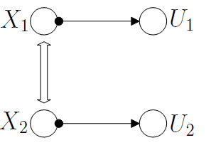
(a)

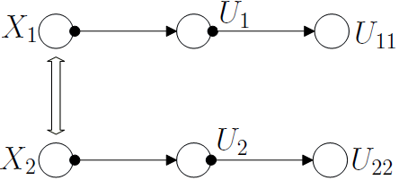
(b)

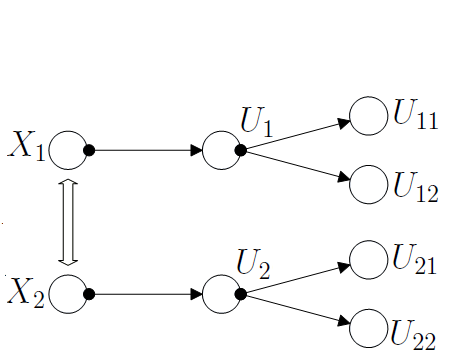
(c)

Figure 9: Depicts the different Markov lemmas.

It was shown in [3] that if a codeword of $U_{1}$ (denoted by $U_{1}^{*}$) is selected jointly typical with $X_{1}^{n}$ and a codeword of $U_{2}$ (denoted by $U_{2}^{*}$) is selected jointly typical with $X_{2}^{n}$ and if $U_{1}\leftrightarrow X_{1}\leftrightarrow X_{2}\leftrightarrow U_{2}$, then $(U_{1}^{*},X_{1}^{n},X_{2}^{n},U_{2}^{*})$ are jointly typical. This is called the generalized Markov lemma and is depicted in Fig. 9a. Similarly, Wagner et al. [10] considered the case in which codewords of $U_{11}$ and $U_{22}$ are generated conditioned on codewords of $U_{1}$ and $U_{2}$, respectively. They showed that if a pair of codewords of $(U_{1},U_{11})$ (denoted by $(U_{1}^{*},U_{11}^{*})$) are jointly typical with $X_{1}^{n}$ and a pair of codewords of $(U_{2},U_{22})$ (denoted by $(U_{2}^{*},U_{22}^{*})$) are typical with $X_{2}^{n}$, and if $(U_{1},U_{11})\leftrightarrow X_{1}\leftrightarrow X_{2}\leftrightarrow(U_{2},U_{22})$, then $(U_{1}^{*},U_{11}^{*},X_{1}^{n},X_{2}^{n},U_{2}^{*}.U_{22}^{*})$ are jointly typical. This is called the conditional Markov lemma for obvious reasons and is depicted in Fig. 9b. However, these results are not sufficient for our scenario and we require a stronger version of the conditional Markov lemma. In what follows, we will establish a series of lemmas, culminating with the needed variant called the conditional Markov lemma for mutual covering (Lemma 3). Note that these lemmas can be easily extended to more than $2$ random variables and layers of encoding. However, we restrict ourselves to the $2$ variable case to keep the notation simple. We also note that the lemmas and proofs here are applicable to more general contexts beyond DIR.

Lemma 1.

Let random variables $(Y,U,V_{1},V_{2})$ be given and let $y^{n}\in\mathcal{T}_{\epsilon}^{n}(Y)$. Let the subset $B_{0}(y^{n})\subset\mathcal{T}_{\epsilon}^{n}(U|y^{n})$ be such that:

$$2^{n(H(U|Y)-\lambda)}\leq|B_{0}(y^{n})|\leq 2^{n(H(U|Y)+\lambda)}$$ (78)

for some $\lambda>0$. For every $u^{n}\in B_{0}(y^{n})$, let subset $B_{12}(y^{n},u^{n})\subset\mathcal{T}_{\epsilon}^{n}((V_{1},V_{2})|u^{n})$ be such that:

$$2^{n(H(V_{1},V_{2}|U,Y)-\lambda)}\leq|B_{12}(y^{n},u^{n})|\leq 2^{n(H(V_{1},V_{2}|U,Y)+\lambda)}$$ (79)

and the following hold:

$$2^{n(H(V_{1}|U,Y)-\lambda)}\leq|B_{1}(y^{n},u^{n})|\leq 2^{n(H(V_{1}|U,Y)+\lambda)}$$

$$2^{n(H(V_{2}|U,Y)-\lambda)}\leq|B_{2}(y^{n},u^{n})|\leq 2^{n(H(V_{2}|U,Y)+\lambda)}$$

$$2^{n(H(V_{1}|U,Y,V_{2})-\lambda)}\leq|\hat{B}_{1}(y^{n},u^{n},v_{2}^{n})|\leq 2^{n(H(V_{1}|U,Y,V_{2})+\lambda)}$$

$$2^{n(H(V_{2}|U,Y,V_{1})-\lambda)}\leq|\hat{B}_{2}(y^{n},u^{n},v_{1}^{n})|\leq 2^{n(H(V_{2}|U,Y,V_{1})+\lambda)}$$ (80)

where $\forall(v_{1}^{n},v_{2}^{n})\in B_{12}(y^{n},u^{n})$:

$$\hat{B}_{1}(y^{n},u^{n},v_{2}^{n}) = \{v_{1}^{n}:(v_{1}^{n},v_{2}^{n})\in B_{12}(y^{n},u^{n})\}$$

$$\hat{B}_{2}(y^{n},u^{n},v_{1}^{n}) = \{v_{2}^{n}:(v_{1}^{n},v_{2}^{n})\in B_{12}(y^{n},u^{n})\}$$

$$B_{1}(y^{n},u^{n}) = \{v_{1}^{n}:\exists(v_{1}^{n},v_{2}^{n})\in B_{12}(y^{n},u^{n})\}$$

$$B_{2}(y^{n},u^{n}) = \{v_{2}^{n}:\exists(v_{1}^{n},v_{2}^{n})\in B_{12}(y^{n},u^{n})\}$$ (81)

Let $R_{0},R_{1}$ and $R_{2}$ be given positive rates. Let $\overline{U}_{j}(j=1,\ldots,2^{nR_{0}})$ be random variables drawn independently and uniformly from $\mathcal{T}_{\epsilon}^{n}(U)$. For each $\overline{U}_{j}$, let $\overline{V}_{jk}^{1}(k=1,\ldots,2^{nR_{1}})$ and $\overline{V}_{jk}^{2}(k=1,\ldots,2^{nR_{2}})$ be random variables drawn independently and uniformly from $\mathcal{T}_{\epsilon}^{n}(V_{1}|\bar{U}_{j})$ and $\mathcal{T}_{\epsilon}^{n}(V_{2}|\bar{U}_{j})$, respectively. Then for $n$ sufficiently large,

$$P\left(\nexists j,k_{1},k_{2}:\overline{U}_{j}\in B_{0}(y^{n}),\,(\bar{V}_{jk_{1}}^{1},\bar{V}_{jk_{2}}^{2})\in B_{12}(y^{n},\overline{U}_{j})\right)$$

$$\leq\delta(\epsilon)$$ (82)

where $\delta(\epsilon)\rightarrow 0$ as $\epsilon\rightarrow 0$, if the rates $R_{0}$,$R_{1}$ and $R_{2}$ satisfy:

$$R_{0} \geq I(Y;U)+7\lambda+19\epsilon$$

$$R_{0}+R_{1} \geq I(Y;V_{1},U)+8\lambda+17\epsilon$$

$$R_{0}+R_{2} \geq I(Y;V_{2},U)+8\lambda+17\epsilon$$

$$R_{0}+R_{1}+R_{2} \geq I(Y;V_{1},V_{2},U)+I(V_{1};V_{2}|U)$$ (83)

$$+6\lambda+15\epsilon$$

Proof.

Define the random variable $\mathcal{X}_{j,k_{1},k_{2}}$ as :

$$\mathcal{X}_{j,k_{1},k_{2}}=\begin{cases}1&\mbox{if }\bar{U}_{j}\in B_{0}(y^{n}),(\bar{V}_{k_{1}}^{1},\bar{V}_{k_{2}}^{2})\in B_{12}(y^{n},\bar{U}_{j})\\ 0&\mbox{else}\end{cases}$$ (84)

Denote by $\mathcal{X}=\sum_{j,k_{1},k_{2}}\mathcal{X}_{j,k_{1},k_{2}}$. Observe that the probability in (82) is equal to $P(\mathcal{X}=0)$. From Chebychev’s inequality, we have:

$$P\left(\mathcal{X}=0\right)\leq\frac{4Var(\mathcal{X})}{(E[\mathcal{X}])^{2}}$$ (85)

Next we have the following from (78) and (79):

$$E[\mathcal{X}] = \sum_{j,k_{1},k_{2}}E[\mathcal{X}_{j,k_{1},k_{2}}]$$

$$=^{(a)} 2^{n(R_{0}+R_{1}+R_{2})}P(\mathcal{X}_{1,1,1})$$

$$\geq 2^{n(R_{0}+R_{1}+R_{2})}\frac{2^{n(H(V_{1},V_{2},U|Y))-2\lambda-5\epsilon)}}{2^{n(H(U)+H(V_{1}|U)+H(V_{2}|U))}}$$

where equality in (a) holds because the random variables $\overline{U}_{j}$, $\overline{V}_{jk}^{1}$ and $\overline{V}_{jk}^{2}$ are drawn independently and uniformly from their respective typical sets. Also, using (79) and (80), we can bound $E[\mathcal{X}^{2}]$ as:

$$E[\mathcal{X}^{2}] = \sum_{j^{1},k_{1}^{1},k_{2}^{1}}\sum_{j^{2},k_{1}^{2},k_{2}^{2}}E[\mathcal{X}_{j^{1},k_{1}^{1},k_{2}^{1}}\mathcal{X}_{j^{2},k_{1}^{2},k_{2}^{2}}]$$ (87)

$$\leq 2^{n(R_{0}+R_{1}+R_{2})}P_{1}+2^{n(R_{0}+2R_{1}+2R_{2})}P_{2}$$

$$+2^{n(R_{0}+2R_{1}+R_{2})}P_{3}+2^{n(R_{0}+R_{1}+2R_{2})}P_{4}$$

$$+2^{2n(R_{0}+R_{1}+R_{2})}P_{1}^{2}$$

where

$$P_{1} = \frac{2^{n(H(V_{1},V_{2},U|Y)+2\lambda+5\epsilon)}}{2^{n(H(U)+H(V_{1}|U)+H(V_{2}|U))}}$$

$$P_{2} = \frac{2^{n(H(U|Y)+2H(V_{1},V_{2}|U,Y)+3\lambda+9\epsilon)}}{2^{n(H(U)+2H(V_{1}|U)+2H(V_{2}|U))}}$$

$$P_{3} = \frac{2^{n(H(V_{1},U|Y)+2H(V_{2}|U,Y,V_{1})+4\lambda+7\epsilon)}}{2^{n(H(V_{1},U)+2H(V_{2}|U))}}$$

$$P_{4} = \frac{2^{n(2H(V_{1}|U,Y,V_{2})+H(V_{2},U|Y))+4\lambda+7\epsilon)}}{2^{n(2H(V_{1}|U)+H(V_{2},U))}}$$ (88)

On substituting (LABEL:eq:Cond_Mark_Ex),(87) and (88) in (85), we have:

$$P\left(\mathcal{X}=0\right)\leq$$

$$4\Bigl{[}\delta(\epsilon)+2^{-n(R_{0}-I(Y;U)-7\lambda-19\epsilon)}$$

$$+2^{-n(R_{0}+R_{1}-I(Y;V_{1},U)-8\lambda-17\epsilon)}$$

$$+2^{-n(R_{0}+R_{2}-I(Y;V_{2},U)-8\lambda-17\epsilon)}$$

$$+2^{-n(R_{0}+R_{1}+R_{2}-I(Y;V_{1},V_{2},U)-I(V_{1};V_{2}|U)-6\lambda-15\epsilon)}\Bigr{]}$$ (89)

which can be made arbitrarily small if the rates satisfy (83). ∎

Lemma 2.

Let $W,Y,U,V_{1}$ and $V_{2}$ be random variables with values in finite sets $\mathcal{W},\mathcal{Y},\mathcal{U},\mathcal{V}_{1}$ and $\mathcal{V}_{2}$, respectively. Let $W^{*}$ be a random variable with values in $\mathcal{W}^{n}$, such that:

$$W^{*}\leftrightarrow Y^{n}\leftrightarrow(U^{n},V_{1}^{n},V_{2}^{n})$$ (90)

Let $R_{0}$, $R_{1}$ and $R_{2}$ be given positive rates. Let $\overline{U}_{i}|_{i=1}^{2^{nR_{0}}}$ denote independent random variables chosen uniformly with replacement from $\mathcal{T}_{\epsilon}^{n}(U)$. Let $\overline{V}_{i,j}^{1}(i=1,\ldots,2^{R_{0}},\,\,j=1,\ldots,2^{nR_{1}})$ and $\overline{V}_{i,j}^{2}(i=1,\ldots,2^{R_{0}},\,\,j=1\ldots 2^{nR_{2}})$ be random variables drawn independently and uniformly from $\mathcal{T}_{\epsilon}^{n}(V_{1}|\overline{U}_{i})$ and $\mathcal{T}_{\epsilon}^{n}(V_{2}|\overline{U}_{i})$, respectively $\forall i$. Further, let,

$$P(W^{*},Y^{n},U^{n},V_{1}^{n},V_{2}^{n}\in\mathcal{T}_{\epsilon}^{n}(W,Y,U,V_{1},V_{2}))\geq 1-\eta$$ (91)

Also, suppose $\forall v_{1}^{n}\in\mathcal{T}_{\epsilon}^{n}(V_{1})$ and $v_{2}^{n}\in\mathcal{T}_{\epsilon}^{n}(V_{2})$:

$$P\left((W^{*},Y^{n},U^{n},V_{1}^{n})\in\mathcal{T}_{\epsilon}^{n}\bigl{|}V_{2}^{n}=v_{2}^{n}\right)\geq 1-\eta$$

$$P\left((W^{*},Y^{n},U^{n},V_{2}^{n})\in\mathcal{T}_{\epsilon}^{n}\bigl{|}V_{1}^{n}=v_{1}^{n}\right)\geq 1-\eta$$ (92)

Then for $n$ sufficiently large, there exists functions $U^{*}(y^{n})$, $V_{1}^{*}(y^{n},U^{*})$ and $V_{2}^{*}(y^{n},U^{*})$, such that:

i) $\overline{U}^{*}(y^{n})=\overline{U}_{i}$ (for some $i\in\{1,\ldots,2^{R_{0}}\}$)$\Rightarrow V_{1}^{*}(y^{n},\overline{U}^{*})=\bar{V}_{i,j_{1}}^{1}$, $V_{2}^{*}(y^{n},\overline{U}^{*})=\bar{V}_{i,j_{2}}^{2}$ for some $j_{1}\in\{1,\ldots,2^{nR_{1}}\}$ and $j_{2}\in\{1,\ldots,2^{nR_{2}}\}$

ii)

$$P((W^{*},Y^{n},\bar{U}^{*},V_{1}^{*},V_{2}^{*})\in\mathcal{T}_{\epsilon}\geq 1-\delta(\epsilon)$$

$$P((W^{*},Y^{n},\bar{U}^{*},V_{1}^{*})\in\mathcal{T}_{\epsilon}\bigl{|}V_{2}^{*})\geq 1-\delta(\epsilon)$$

$$P((W^{*},Y^{n},\bar{U}^{*},V_{2}^{*})\in\mathcal{T}_{\epsilon}\bigl{|}V_{1}^{*})\geq 1-\delta(\epsilon)$$ (93)

for some $\delta(\epsilon)\rightarrow 0$ as $\epsilon\rightarrow 0$, if the rates $R_{0}$,$R_{1}$ and $R_{2}$ satisfy:

$$R_{0} \geq I(Y;U)+40\epsilon$$

$$R_{0}+R_{1} \geq I(Y;V_{1},U)+41\epsilon$$

$$R_{0}+R_{2} \geq I(Y;V_{2},U)+41\epsilon$$ (94)

$$R_{0}+R_{1}+R_{2} \geq I(Y;V_{1},V_{2},U)+I(V_{1};V_{2}|U)+33\epsilon$$

Proof.

Let us expand (91) as:

$$\sum_{y^{n}\in\mathcal{Y}^{n}}\Bigl{\{}P\Bigl{(}(W^{*},U^{n},V_{1}^{n},V_{2}^{n})\in\mathcal{T}_{\epsilon}^{n}\Bigl{|}Y^{n}=y^{n}\Bigr{)}$$

$$P(Y^{n}=y^{n})\Bigr{\}}\geq 1-\eta$$

(95)

Let,

$$A\triangleq\Bigl{\{}y^{n}:P\Bigl{(}(W^{*},U^{n},V_{1}^{n},V_{2}^{n})\in\mathcal{T}_{\epsilon}^{n}\Bigl{|}Y^{n}=y^{n}\Bigr{)}$$

$$\geq 1-\sqrt{\eta}\Bigr{\}}$$

and

$$A_{0}\triangleq A\bigcap\mathcal{T}_{\epsilon}^{n}(Y)$$ (96)

Then using the reverse Markov inequality, we can show that (similar to [3, 10]):

$$P(Y^{n}\in A_{0})\geq 1-\delta_{1}$$ (97)

where $\delta_{1}=\sqrt{\eta}+\epsilon$. Then for any $y^{n}\in A_{0}$, we have:

$$\sum_{u^{n}}\Bigl{\{}P\Bigl{(}(W^{*},V_{1}^{n},V_{2}^{n})\in\mathcal{T}_{\epsilon}^{n}\Bigl{|}Y^{n}=y^{n},U^{n}=u^{n}\Bigr{)}$$

$$P\Bigl{(}U^{n}=u^{n}\Bigl{|}Y^{n}=y^{n}\Bigr{)}\Bigr{\}}\geq 1-\sqrt{\eta}$$ (98)

Let,

$$B(y^{n})\triangleq\Bigl{\{}u^{n}:P\Bigl{(}(W^{*},V_{1}^{n},V_{2}^{n})\in\mathcal{T}_{\epsilon}^{n}\Bigl{|}Y^{n}=y^{n},U^{n}=u^{n}\Bigr{)}$$

$$\geq 1-\sqrt[4]{\eta}\Bigr{\}}$$

$$B_{0}\triangleq B\bigcap\mathcal{T}_{\epsilon}^{n}(U|y^{n})$$ (99)

Using the reverse Markov inequality, we again have:

$$P\Bigl{(}U^{n}\in B_{0}(y^{n})\Bigl{|}Y^{n}=y^{n}\Bigr{)}\geq 1-\delta_{2}$$ (100)

where $\delta_{2}=\sqrt[4]{\eta}+\epsilon$. Hence for any $y^{n}\in A_{0}$ and $u^{n}\in B_{0}(y^{n})$ we have:

$$\sum_{u^{n},v_{1}^{n},v_{2}^{n}}P\Bigl{(}V_{1}^{n}=v_{1}^{n},V_{2}^{n}=v_{2}^{n}\Bigl{|}Y^{n}=y^{n},U^{n}=u^{n}\Bigr{)}$$

$$Q(y^{n},u^{n},v_{1}^{n},v_{2}^{n})\geq 1-\sqrt[4]{\eta}$$ (101)

where we denote by $Q(\mathcal{S})$$=P\Bigl{(}W^{*}\in\mathcal{T}_{\epsilon}^{n}(W|\mathcal{S})\Bigl{|}Y^{n}=y^{n}\Bigr{)}$ for any set of sequences $\mathcal{S}$. Note that we have used the Markov condition (90) in the above equation. Now define sets $\tilde{B}_{12}(y^{n},u^{n})$ and $B_{12}(y^{n},u^{n})$ for any $y^{n}\in A_{0}$ and $u^{n}\in B_{0}(y^{n})$ such that:

$$\tilde{B}_{12}(y^{n},u^{n})\triangleq\Bigl{\{}(v_{1}^{n},v_{2}^{n}):Q(y^{n},u^{n},v_{1}^{n},v_{2}^{n})\geq 1-\sqrt[8]{\eta}\Bigr{\}}$$

$$B_{12}(y^{n})\triangleq\tilde{B}_{12}(y^{n})\bigcap\mathcal{T}_{\epsilon}^{n}(U,V_{1},V_{2}|y^{n})$$ (102)

Then using the reverse Markov inequality, we can show that:

$$P\Bigl{(}(V_{1}^{n},V_{2}^{n})\in B_{12}(y^{n})\Bigl{|}Y^{n}=y^{n},U^{n}=u^{n}\Bigr{)}\geq 1-\delta_{3}$$ (103)

where $\delta_{3}=\sqrt[8]{\eta}+\epsilon$. Then from (100), (103) and Lemma 3.1(f) in [3], for $n$ sufficiently large, we have:

$$2^{n(H(U|Y)-3\epsilon)} \leq|B_{0}(y^{n})|\leq 2^{n(H(U|Y)+\epsilon)}$$

$$2^{n(H(V_{1},V_{2}|Y,U)-3\epsilon)} \leq|B_{12}(y^{n},u^{n})|\leq 2^{n(H(V_{1},V_{2}|Y,U)+\epsilon)}$$ (104)

Note that we have two of the sets required by Lemma 1. However, we further require bounds on the projections of $B_{12}(y^{n},u^{n})$ (as in (80)) to invoke Lemma 1. Towards obtaining these bounds, we note that the following inequalities can be shown directly from (91):

$$P\left((W^{*},Y^{n},U^{n},V_{1}^{n})\in\mathcal{T}_{\epsilon}^{n}\right)\geq 1-\eta$$

$$P\left((W^{*},Y^{n},U^{n},V_{2}^{n})\in\mathcal{T}_{\epsilon}^{n}\right)\geq 1-\eta$$ (105)

Expanding (105) instead of (91) and repeating all steps from (95) through (104), we obtain:

$$2^{n(H(V_{1}|Y,U)-3\epsilon)} \leq|B_{1}(y^{n},u^{n})|\leq 2^{n(H(V_{1}|Y,U)+\epsilon)}$$

$$2^{n(H(V_{2}|Y,U)-3\epsilon)} \leq|B_{2}(y^{n},u^{n})|\leq 2^{n(H(V_{2}|Y,U)+\epsilon)}$$ (106)

where

$$B_{1}(y^{n},u^{n}) =\{v_{1}^{n}:\exists(v_{1}^{n},v_{2}^{n})\in B_{12}(y^{n},u^{n})\}$$

$$B_{2}(y^{n},u^{n}) =\{v_{2}^{n}:\exists(v_{1}^{n},v_{2}^{n})\in B_{12}(y^{n},u^{n})\}$$ (107)

Similarly, it is easy to show that expanding (92) instead of (91) leads to:

$$2^{n(H(V_{1}|Y,U,V_{2})-3\epsilon)} \leq|\hat{B}_{1}(y^{n},u^{n},v_{2}^{n})|\leq 2^{n(H(V_{1}|Y,U,V_{2})+\epsilon)}$$

$$2^{n(H(V_{2}|Y,U,V_{1})-3\epsilon)} \leq|\hat{B}_{2}(y^{n},u^{n},v_{1}^{n})|\leq 2^{n(H(V_{2}|Y,U,V_{1})+\epsilon)}$$ (108)

where $\forall v_{1}^{n}\in B_{1}(y^{n},u^{n})$ and $v_{2}^{n}\in B_{2}(y^{n},u^{n})$,

$$\hat{B}_{1}(y^{n},u^{n},v_{2}^{n}) =\{v_{1}^{n}:(v_{1}^{n},v_{2}^{n})\in B_{12}(y^{n},u^{n})\}$$

$$\hat{B}_{2}(y^{n},u^{n},v_{1}^{n}) =\{v_{2}^{n}:(v_{1}^{n},v_{2}^{n})\in B_{12}(y^{n},u^{n})\}$$ (109)

We now have sets $B_{0}$ and $B_{12}$ satisfying all the bounds as required in Lemma 1. Hence, we can define the functions $U^{*},V_{1}^{*}$ and $V_{2}^{*}$ as follows. $U^{*}(y^{n})=\overline{U}_{i}$ if $\bar{U}_{i}\in B_{0}(y^{n})$. If no such $\bar{U}_{i}$ exists, we set $U^{*}(y^{n})=\bar{U}_{1}$. Next, if there exists a pair $(\overline{V}_{i,j_{1}}^{1},\overline{V}_{i,j_{2}}^{2})$ such that $(\overline{V}_{i,j_{1}}^{1},\overline{V}_{i,j_{2}}^{2})\in B_{12}(y^{n},\overline{U}_{i})$, then define $(V_{1}^{*}(y^{n},U^{*}),V_{2}^{*}(y^{n},U^{*}))=(\overline{V}_{i,j_{1}}^{1},\overline{V}_{i,j_{2}}^{2})$. If there exists no such pair, define $(V_{1}^{*}(y^{n},U^{*}),V_{2}^{*}(y^{n},U^{*}))=(\overline{V}_{i,1}^{1},\overline{V}_{i,1}^{2})$.

It follows from the rate conditions in (94), Lemma 1 with $\lambda=3\epsilon$ and the bounds on set sizes that:

$$P\left(U^{*}\in B_{0}(Y^{n}),(V_{1}^{*},V_{2}^{*})\in B_{12}(Y^{n},U^{*})\Bigl{|}Y^{n}\in A_{0}\right)$$

$$\geq 1-\delta(\epsilon)$$ (110)

for some $\delta(\epsilon)\rightarrow 0$ as $\epsilon\rightarrow 0$. Note that $y^{n}\in A_{0}$, $U^{*}\in B_{0}(Y^{n})$ and $(V_{1}^{*},V_{2}^{*})\in B_{12}(Y^{n},U^{*})$ imply that $(y^{n},U^{*},V_{1}^{*},V_{2}^{*})\in\mathcal{T}_{\epsilon}^{n}(Y,U,V_{1},V_{2})$. We then have,

$$P(W^{*},Y^{n},U^{*},V_{1}^{*},V_{2}^{*}\in T_{\epsilon}^{n})\geq P(E_{1})P(E_{2}|E_{1})$$ (111)

where events $E_{1}$ and $E_{2}$ are defined as:

$$E_{1} = \{Y^{n}\in A_{0},U^{*}\in B_{0},(V_{1}^{*},V_{2}^{*})\in B_{12}\}$$

$$E_{2} = \{W^{*}\in T_{\epsilon}^{n}(W|Y^{n},U^{*},V_{1}^{*},V_{2}^{*})\}$$ (112)

From (97), (103) and (102), we obtain bounds on $P(E_{1})$ and $P(E_{2}|E_{1})$:

$$P(E_{1}) \geq 1-\delta_{1}-\delta_{2}-\delta_{3}$$

$$P(E_{2}|E_{1}) \geq 1-\sqrt[8]{\eta}$$ (113)

On substituting in (111), we obtain the first bound in (93). The other two bounds in (93) can be shown using similar arguments.∎

Lemma 3.

Conditional Markov Lemma - for Mutual Covering: Suppose that $(X_{1},X_{2},U_{1},U_{2},U_{11},U_{12},U_{21},U_{22})$ are random variables taking values in arbitrary finite sets $(\mathcal{X}_{1},\mathcal{X}_{2},\mathcal{U}_{1},\mathcal{U}_{2},\mathcal{U}_{11},\mathcal{U}_{12},\mathcal{U}_{21},\mathcal{U}_{22})$, respectively. Let the random variables satisfy the following Markov condition:

$$(U_{1},U_{11},U_{12})\leftrightarrow X_{1}\leftrightarrow X_{2}\leftrightarrow(U_{2},U_{21},U_{22})$$ (114)

Let $\overline{U}_{1,i}:i=1,\ldots,2^{nR_{1}}$ and $\overline{U}_{2,i}:i=1,\ldots,2^{nR_{2}}$ be independent codewords of length $n$ each generated using the marginals $P(U_{1})$ and $P(U_{2})$, respectively. Let $2^{nR_{11}}$ and $2^{nR_{12}}$ codewords of $U_{11}$ and $U_{12}$ (denoted by $\overline{U}_{11,ij}$ and $\overline{U}_{12,ij}$), respectively, be generated conditioned on each codeword $\overline{U}_{1,i}$. Similarly generate codewords of $U_{21}$ and $U_{22}$ at rates $R_{21}$ and $R_{22}$, respectively, conditioned on the codewords of $U_{2}$. Then for $n$ sufficiently large, there exists functions $U_{1}^{*}(X_{1}^{n})$,$U_{2}^{*}(X_{2}^{n})$, $U_{11}^{*}(X_{1}^{n},U_{1}^{*})$,$U_{12}^{*}(X_{1}^{n},U_{1}^{*})$,$U_{21}^{*}(X_{2}^{n},U_{2}^{*})$ and $U_{22}^{*}(X_{2}^{n},U_{2}^{*})$ taking values in $\mathcal{U}_{1}^{n},\mathcal{U}_{2}^{n},\mathcal{U}_{11}^{n},\mathcal{U}_{12}^{n},\mathcal{U}_{21}^{n}$ and $\mathcal{U}_{22}^{n}$, respectively, such that:

$$P\left((X_{1}^{n},X_{2}^{n},U_{1}^{*},U_{2}^{*},U_{11}^{*},U_{12}^{*},U_{21}^{*},U_{22}^{*})\in\mathcal{T}_{\epsilon}^{n}\right)\geq 1-\delta(\epsilon)$$ (115)

where $\delta(\epsilon)\rightarrow 0$ as $\epsilon\rightarrow 0$ if the rates satisfy:

$$R_{1} > I(X_{1};U_{1}),$$

$$R_{2} > I(X_{2};U_{2})$$

$$R_{1}+R_{11} > I(X_{1};U_{11},U_{1}),$$

$$R_{1}+R_{12} > I(X_{1};U_{12},U_{1}),$$

$$R_{2}+R_{21} > I(X_{2};U_{21},U_{2}),$$

$$R_{2}+R_{22} > I(X_{2};U_{22},U_{2}),$$

$$R_{1}+R_{11}+R_{12} > I(X_{1};U_{11}U_{12},U_{1})$$

$$+I(U_{11};U_{12}|U_{1}),$$

$$R_{2}+R_{22}+R_{21} > I(X_{2};U_{21},U_{22},U_{2})$$ (116)

$$+I(U_{21};U_{22}|U_{2})$$

Note that this lemma can be easily extended to the more general case of multiple random variables and multiple layers of encoding using induction (see [3] for the general methodology). While we use the more general version in the proof of Theorem 1 in Appendix Appendix A: Bounding Encoding/Decoding Errors in Theorem 1, we restrict to the simpler case here for ease of understanding and to avoid complex notation.

Proof.

We note that from standard arguments [8, 35, 2], it follows that if the rates satisfy (116), then there exists functions $U_{1}^{*}(X_{1}^{n})$, $U_{11}^{*}(X_{1}^{n},U_{1}^{*})$ and $U_{12}^{*}(X_{1}^{n},U_{1}^{*})$ such that:

$$P\left((X_{1}^{n},U_{1}^{*},U_{11}^{*},U_{12}^{*})\in\mathcal{T}_{\epsilon}^{n}\right)\geq 1-\delta(\epsilon)$$ (117)

for some $\delta(\epsilon)\rightarrow 0$ as $\epsilon\rightarrow 0$. Also, note that $X_{2}^{n}$ is drawn according to the right conditional PMF given $X_{1}^{n}$. Hence, we have:

$$P\left((X_{1}^{n},X_{2}^{n},U_{1}^{*},U_{11}^{*},U_{12}^{*})\in\mathcal{T}_{\epsilon}^{n}\right)\geq 1-\delta(\epsilon)$$ (118)

What remains for us to show is that there exists functions $U_{2}^{*}(X_{2}^{n})$, $U_{21}^{*}(X_{2}^{n},U_{2}^{*})$ and $U_{22}^{*}(X_{2}^{n},U_{2}^{*})$, taking values in $\mathcal{U}_{2}^{n},\mathcal{U}_{21}^{n},\mathcal{U}_{22}^{n}$, jointly typical with $X_{1}^{n},X_{2}^{n},U_{1}^{*},U_{11}^{*},U_{12}^{*}$. We invoke Lemma 2 with $W^{*}=(X_{1}^{n},U_{1}^{*},U_{11}^{*},U_{12}^{*})$, $Y^{n}=X_{2}^{n}$, $U=U_{2}$, $V_{1}=U_{21}$ and $V_{2}=U_{22}$. Note that given (116) and (118), conditions (90),(91) and (92) are satisfied (for a formal proof of this claim, refer to [35]). Hence, it follows from Lemma 2 that there exist functions $U_{2}^{*}(X_{2}^{n})$, $U_{21}^{*}(X_{2}^{n},U_{2}^{*})$ and $U_{22}^{*}(X_{2}^{n},U_{2}^{*})$ such that:

$$P\left((X_{1}^{n},X_{2}^{n},U_{1}^{*},U_{2}^{*},U_{11}^{*},U_{12}^{*},U_{21}^{*},U_{22}^{*})\in\mathcal{T}_{\epsilon}^{n}\right)\geq 1-\delta(\epsilon)$$ (119)

thus proving the lemma. ∎

References

• [1] R. Cristescu, B. Beferull-Lozano, and M. Vetterli, “Networked Slepian-Wolf: Theory, algorithms and scaling laws,” IEEE Trans. on Information Theory, vol. 51, no. 12, pp. 4057–4073, Dec 2005.
• [2] R. Venkataramani, G. Kramer, and V. Goyal, “Multiple descriptions coding with many channels,” IEEE Trans. on Information Theory, vol. 49, no. 9, pp. 2106–2114, Sep 2003.
• [3] T. S. Han and K. Kobayashi, “A unified achievable rate region for a general class of multiterminal source coding systems,” IEEE Trans. on Information Theory, vol. IT-26, pp. 277–288, May 1980.
• [4] D. Slepian and J. K. Wolf, “Noiseless coding of correlated information sources,” IEEE Trans. on Information Theory, vol. 19, pp. 471–480, Jul 1973.
• [5] A. D. Wyner and J. Ziv, “The rate-distortion function for source coding with side information at the decoder,” IEEE Trans. on Information Theory, vol. 22, pp. 1–10, Jan 1976.
• [6] T. Berger, Multiterminal source coding.   lecture note presented at CISM, Udine, Italy, 1977.
• [7] T. M. Cover, “A proof of the data compression theorem of Slepian and Wolf for ergodic sources,” IEEE Trans. on Information Theory, vol. IT-21, pp. 226–228, Mar 1975.
• [8] A. Gamal and T. M. Cover, “Achievable rates for multiple descriptions,” IEEE Trans. on Information Theory, vol. IT-28, pp. 851–857, Nov 1982.
• [9] S. Tung, Multiterminal source coding.   Ph.D. dissertation, School of Electrical Engineering, Cornell University, Ithaca, NY, 1978.
• [10] A. Wagner, B. Kelly, and Y. Altug, “Distributed rate-distortion with common components,” IEEE Trans. on Information Theory, vol. 57, no. 7, pp. 4035–4057, Jul 2011.
• [11] A. Wyner, “The common information of two dependent random variables,” IEEE Trans. on Information Theory, vol. 21, pp. 163 – 179, Mar 1975.
• [12] Z. Zhang and T. Berger, “New results in binary multiple descriptions,” IEEE Trans. on Information Theory, vol. IT-33, pp. 502–521, Jul 1987.
• [13] R. Gray and A. Wyner, “Source coding over simple networks,” Bell Systems Tech. Journal, vol. 53, no. 9, pp. 1681–1721, Nov. 1974.
• [14] A. Wyner, “On source coding with side information at the decoder,” IEEE Trans. on Information Theory, vol. IT 21, no. 3, pp. 294–300, May 1975.
• [15] I. Csisz$\mathrm{\acute{a}}$r and J. K$\mathrm{\ddot{o}}$rner, “Towards a general theory of source networks,” IEEE Trans. on Information Theory, vol. 26, pp. 155–165, Mar 1980.
• [16] H. Luo, Y. Liu, and S. K. Das, “Routing correlated data in wireless sensor networks: A survey,” IEEE Network, vol. 21, no. 6, pp. 40–47, Dec 2007.
• [17] R. Cristescu, B. Beferull-lozano, M. Vetterli, and R. Wattenhofer, “Network correlated data gathering with explicit communication: NP completeness and algorithms,” IEEE/ACM Trans. on Networking, vol. 14, pp. 41–54, 2006.
• [18] S. Pattem, B. Krishnamachari, and R. Govindan, “The impact of spatial correlation on routing with compression in wireless sensor networks,” IEEE Trans. on Sensor Networks, vol. 4, no. 4, 2008.
• [19] T. Cormen, C. Leiserson, and R. Rivest, Introduction to algorithms.   McGraw-Hill Science/Engineering/Math, Jul 2001.
• [20] J. Liu, M. Adler, D. Towsley, and C. Zhang, “On optimal communication cost for gathering correlated data through wireless sensor networks,” in Proceedings of the 12th ACM Annual International Conference on Mobile Computing and Networking, Sep 2006, pp. 310–321.
• [21] K. Viswanatha, E. Akyol, and K. Rose, “Towards optimum cost in multi-hop networks with arbitrary network demands,” in IEEE International Symposium on Information Theory (ISIT), Jun 2010, pp. 1833–1837.
• [22] ——, “On optimum communication cost for joint compression and dispersive information,” in IEEE Information Theory Workshop (ITW), Sep 2010, pp. 1–5.
• [23] ——, “An achievable rate region for distributed source coding and dispersive information routing,” in IEEE International Symposium on Information Theory (ISIT), Aug 2011, pp. 776–780.
• [24] D. S. Lun, M. Medard, T. Ho, and R. Koetter, “Network coding with a cost criterion,” in Proceedings of International Symposium on Information Theory and its Applications, 2004, pp. 1232–1237.
• [25] A. Ramamoorthy, “Minimum cost distributed source coding over a network,” IEEE Trans. on Information Theory, vol. 57, no. 1, Jan 2011.
• [26] T. M. Cover and J. A. Thomas, Elements of information theory.   Wiley-Interscience, 1991.
• [27] P. G$\mathrm{\acute{a}}$cs and J. K$\mathrm{\ddot{o}}$rner, “Common information is far less than mutual information,” Problems of Control and Information Theory, 1973.
• [28] R. Timo, A. Grant, T. Chan, and G. Kramer, “Source coding for a simple network with receiver side information,” in IEEE International Symposium on Information Theory (ISIT), Jul 2008, pp. 2307–2311.
• [29] A. Wyner, J. Wolf, and F. Willems, “Communicating via processing broadcast satellite,” IEEE Trans. on Information Theory, vol. 48, pp. 1243–1249, Jun 2002.
• [30] R. Timo, A. Grant, and L. Hanlen, “Source coding for a noiseless broadcast channel with partial receiver side information,” in IEEE Australian Communications Theory Workshop, Feb 2007.
• [31] K. Viswanatha, E. Akyol, S. Ramaswamy, and K. Rose, “Distributed source coding and dispersive information routing: An integrated approach with networking and database applications,” in European Signal Processing Conference (EUSIPCO), Aug 2010, pp. 1894–1898.
• [32] J. K$\mathrm{\ddot{o}}$rner and K. Marton, “How to encode the modulo-two sum of binary sources (Corresp.),” IEEE Trans. on Information Theory, vol. 25, pp. 219– 221, Mar 1979.
• [33] R. Ahlswede and J. K$\mathrm{\ddot{o}}$rner, “Source coding with side information and a converse for degraded broadcast channels,” IEEE Trans. on Information Theory, vol. IT-21, pp. 629–637, Nov 1975.
• [34] D. Marco and M. Effros, “On lossless coding with coded side information,” IEEE Trans. on Information Theory, vol. 55 (7), pp. 3284–3296, 2009.
• [35] A. Gamal and Y. Kim, Network information theory.   Cambridge University Press, 2011.