The naked emergence of solar active regions observed with SDO/HMI

Abstract

We take advantage of the HMI/SDO instrument to study the naked emergence of active regions from the first imprints of the magnetic field on the solar surface. To this end, we followed the first 24 hours in the life of two rather isolated ARs that appeared on the surface when they were about to cross the central meridian. We analyze the correlations between Doppler velocities and the orientation of the vector magnetic field finding, consistently, that the horizontal fields connecting the main polarities are dragged to the surface by relatively-strong upflows and are associated to elongated granulation that is, on average, brighter than its surroundings. The main magnetic footpoints, on the other hand, are dominated by vertical fields and downflowing plasma. The appearance of moving dipolar features, MDFs, (of opposite polarity to that of the AR) in between the main footpoints, is a rather common occurrence once the AR reaches a certain size. The buoyancy of the fields is insufficient to lift up the magnetic arcade as a whole. Instead, weighted by the plasma that it carries, the field is pinned down to the photosphere at several places in between the main footpoints, giving life to the MDFs and enabling channels of downflowing plasma. MDF poles tend to drift towards each other, merge and disappear. This is likely to be the signature of a reconnection process in the dipped field lines, which relieves some of the weight allowing the magnetic arcade to finally rise beyond the detection layer of the HMI spectral line.

1 Active region emergence

Solar active regions have puzzled humanity for millenia. The work of Hale (1908) established that sunspots harbour strong magnetic fields, which, together with other observations of the properties of the solar cycle, set the basis for the current theories of solar dynamo. Although specific details of the emergence of active regions (AR) are still a matter of research, the established paradigm says that their magnetic field is generated close to the base of the convection zone. Then, presumably triggered by deep convective flows and buoyant instabilities, these magnetic fields rise towards the surface, protrude through it and leave footprints in the form of sunspots and plage (see, for instance, the reviews by Moreno-Insertis, 1997; Fan, 2009).

Observationally, active region emergence sites have been the object of many studies. Most of these works, especially the ones from the earlier days, made use of intensity and circular polarization measurements, which restricted the inference of the magnetic field vector to its longitudinal component only (i.e. projected along the line-of-sight, LOS).

A series of papers (Zwaan, 1985; Brants, 1985a, b; Brants & Steenbeek, 1985) marked the starting point for the analysis of the magnetic and dynamic properties of the emergence process. Based on the width and Doppler shifts of the Stokes I profiles, they inferred $\sim 500{\rm G}$ transverse magnetic fields associated to small-scale upflows in the photosphere, which they interpreted to be the signatures of the top of the flux loops reaching the surface. They observed strong downflows in the vicinity of rapidly growing pores, but no systematic flows within the pores themselves. They also reported the existence of very strong (1000-2000G) transverse fields, result which was later questioned by Lites et al. (1998) on the basis of the limitations in the determination of the transverse component of the magnetic field using only intensity and circular polarization measurements. Strous (1994) and Strous & Zwaan (1999) saw elongated darkenings in the photospheric continuum intensity at emergence sites associated to $0.5{\rm kms^{-1}}$ upflows. These darkenings were almost aligned with the orientation of the AR, which lead the authors to interpret them as being the crests of undulatory flux tubes penetrating the photosphere.

Lites et al. (1998) used full Stokes measurements of small emerging bipolar regions to determine the properties of the magnetic field vector. They found horizontal fields of 200-600 Gauss associated to small transient upflows at the site of the emergence, suggesting that there is a canopy of weak horizontal magnetic fields over-arching the emergence zone. Small flux elements constantly drift away from the emergence site and attain kiloGauss strengths only when they become almost vertically oriented. Kubo et al. (2003) derived magnetic filling factors of around 80% at the emergence site, indicating that the horizontal fields of the tops of the magnetic arcades are intrinsically weak.

Bernasconi et al. (2002) reported on small moving dipolar features (MDFs) of opposite polarity to that of the active region, that appear in the midst of the emerging sites. They found that these features tended to flow into sunspots and supergranule boundaries. The authors identified MDFs as stitches where the emerging flux ropes were still tied to the photosphere by trapped mass, giving the emerging field a serpentine nature. Vargas Domínguez et al. (2012) observed small-scale short-lived dark features followed by brightenings in the low chromosphere associated to these serpentine fields. They were interpreted as signatures of the energy release due to reconnection of U-loops and elementary arch filament systems rising up into the chromosphere. Watanabe et al. (2008) suggested that the emergence of flux tubes inside active regions is a triggering mechanism of Ellerman bombs. They proposed several scenarios in which the newly emerged magnetic fields either interact with pre-existing fields or suffer reconnections within their dipped arcade structures. In both cases, the magnetic reconnection happens in the chromosphere, releasing the energy responsible for the observed Ellerman Bombs.

There are quite a few works that focus on the velocity flows in young emerging active regions. While it is accepted that systematic velocities in the umbrae of mature sunspots are insignificant, the flows during their formation seem to be a matter of debate. From the observational point of view, there has been a range of qualitatively different results over the last few decades. Symmetric downflows at the footpoints of individual emerging loops were reported by Brants (1985b). However, asymmetries in the flows have also been reported by several authors. From the predominant downflows in the leading part of young active regions found by Walton et al. (1994) and later Cauzzi et al. (1996), to the upwelling velocities in the umbra of a following sunspot pointed out by Sigwarth et al. (1998), obsevations in this respect seem to be non-conclusive.

Numerical simulations of the formation of ARs focus either on the deep convection zone or the uppermost 10 Mm and the photosphere. This is due to the huge range of time- and length-scales involved in the process. Fully compressible MHD simulations of the emergence of ARs in the last 10-20 Mm below the photosphere try to explain the rise of magnetic flux through a highly stratified atmosphere and the subsequent formation of coherent sunspots of kilo-Gauss strengths. By letting a buoyant, twisted semi-torus flux tube be kinematically advected into the computational domain, Cheung et al. (2010) have rather successfully achieved to explain the formation of an AR and some of the associated observational properties (elongated granules, mixed polarity patterns in the emergence zone, pore formation and light bridges). Stein et al. (2011a) and Stein et al. (2011b) studied a complementary situation where a uniform, untwisted, horizontal field is advected into the computational domain by convective inflows through a depth of 20 Mm. In their simulations, a large-scale magnetic loop emerges through the surface leading to the formation of a bipolar pore-like structure.

There is a tendency for new flux to emerge within - or in the vicinity of - existing active regions (see, for instance, Zhang et al., 2012; MacTaggart, 2011; Lites et al., 2010; Zuccarello et al., 2008), which indicates that the underlying toroidal field is already disturbed and likely to erupt again (van Ballegooijen, 2008). A vast majority of the existing observations of newly emerged magnetic flux takes place in this scenario. Observations reliant on non-synoptic instruments are very unlikely to capture the naked emergence of an AR. In the context of this paper, the attribute naked refers to flux emergence that is isolated from and unrelated to, pre-existing magnetic activity. This particular characteristic makes it possible to study the properties of emergence independently of the interaction with large-scale pre-existing fields. In order to comprehensively understand the properties of these emergence sites, the evolution of the full vector magnetic field needs to be measured. The Helioseismic and Magnetic Imager (HMI) suits the bill perfectly. Unlike any other instrument before, it provides uninterrupted, high cadence photospheric vector magnetic field and Doppler velocities of the full solar disk, rendering it possible to study the magnetic and dynamic properties of active regions from their very first stages of emergence, as long they appear on the visible disk.

In this paper we attempt to compile the main properties of the “naked” emergence of active regions as seen by HMI. The particularities of the chosen datasets and a comprehensive study of their advantages and limitations are analyzed in Section 2. In section 3, the evolution of different magnetic and dynamic aspects observed during the first stages of emergence are described and discussed, and a consistent scenario is put together in section 4.

2 Observations and data reduction

In this paper we analyze the properties of two relatively isolated active regions that emerged when they were about to cross the central meridian of the solar disk. The data were taken by the vector camera of the HMI instrument (Schou et al., 2012) on board the Solar Dynamics Observatory (SDO, Pesnell et al., 2012), which provides continuous full disk measurements of the Stokes vector of the photospheric Fe i 6173 Å line every $\sim 135$ seconds. Although this is the native cadence, the standard HMI vector products correspond to averages in 16-minute tapered windows, rendering a final cadence of 12 minutes. HMI is a filter instrument. The full width at half maximum (FWHM) of the HMI filtergrams is  76 mÅ and the spectral line is sampled at six equispaced wavelength positions. The spatial resolution of the HMI data is of $\sim 1\arcsec$ ($0.5\arcsec$ pixel) and the polarimetric sensitivity about $\sim 1.2\cdot 10^{-3}$ times continuum intensity.

The standard pipeline calibration and the spectral line inversion (Very Fast Inversion of the Stokes Vector (VFISV), Borrero et al., 2011) of 12-minute averages were used to compute the photospheric vector magnetic field quantities and Doppler velocities (see section 2.1).

	date & initial	hemisphere	approx. position	average $\mu$
	emergence time
AR 11105	Sep 1, 2010 @ 20:00UT	North	20N 5E	0.975
AR 11211	May 7, 2011 @ 23:00UT	South	13S 10E	0.982

Table 1: Details of the two datasets presented in this paper.

Details of the datasets can be found in table 1. Two active regions, AR 11105 and AR 11211, were followed for 24 hours after the first signatures of emergence were detected. Of course, the magnetic signature precedes any darkening in the continuum intensity, so we consider the beginning of the process to happen when magnetograms show the first hints of activity, beyond the signals of pre-existing network patches. SDO has been collecting data since April 2010. These particular events were selected from a very wealthy dataset for two reasons: 1, they were both relatively isolated from pre-existing active regions and 2, they took place very close to disk center, where projection effects are minimal (the average heliocentric angle, $\mu$, of the center of each AR over the first 24 hours of its life is listed in table 1). Not intending to carry out a statistical study of the properties of active region emergence, we do attempt to sample regions with significantly different flux output. Whilst AR 11105 grew quickly and developed into a full grown system with sunspots and pores, AR11211 generated a few tiny pores and decayed within a matter of days, before leaving the visible disk.

2.1 The spectral line inversion

In order to obtain the magnetic field and Doppler velocities at the Photosphere, the HMI full Stokes data were processed with the VFISV spectral line inversion code (Borrero et al., 2011). This code inverts the polarized radiative transfer equation assuming that the solar atmosphere can be represented by the Milne-Eddington (ME) approximation and that the generation of polarized radiation takes place within the classical Zeeman effect regime. These assumptions impose stringent constraints on the possible solutions for the model atmosphere and lead to limitations in the interpretation of the Stokes profiles. A Milne-Eddington model assumes that all of the physical parameters that describe the atmosphere are constant along the line of sight, except for the source function, which varies linearly with the optical depth. Asymmetries of the Stokes profiles cannot be interpreted in the context of this approximation since no gradients in the velocity or the magnetic field are allowed. Although no depth dependence for the inverted parameters is obtained, the results are representative of the average physical properties of the atmosphere in the region of formation of the spectral line (Westendorp Plaza et al., 1998).

VFISV operates assuming a magnetic filling factor of unity, $\alpha=1$, where $\alpha$ is the fraction of the area of the pixel that contains magnetic field. This means that each pixel is considered to be fully magnetized rather than composed of a magnetic and a non-magnetic components. This assumption has a different effect on the longitudinal and the transverse components of the retrieved magnetic field but, in general, it leads to an underestimation of the field strength and a biasing of the inclinations towards more horizontal configurations (see, for instance, the discussion in Sánchez Almeida & Martínez González, 2011).

No magnetic field disambiguation was applied to the datasets. The magnetic field inclinations, $\theta_{B}$, reported in this paper refer to the line-of-sight and the azimuth angles, $\chi_{B}$, vary between 0 and 180 degrees in the plane perpendicular to the LOS. Because during the time span of the observations presented in this paper neither of the ARs was far away from disk center (the heliocentric angle, $\mu$, was always larger than 0.97; see table 1), the two solutions for the azimuth of the magnetic field should yield inclinations with respect to the local vertical that do not differ much with those calculated with respect to the LOS.

Photon noise that propagates thorough the spectral line inversion process results in uncertainties in the magnetic field parameters derived by the inversion. The transverse component of the magnetic field vector is much more sensitive to this than the longitudinal component. But random noise is not the only contributor to the uncertainties. There are systematic effects that come from the instrument and from the inversion algorithm that are more difficult to characterize. The instrumental effects produce variations in time, with periods that are related to the orbital motion of the satellite. If we take a statistically significant sample of pixels whose polarization profiles are pure noise and we give them to the inversion code, the resulting average field strength will vary between 70 and 100 G, as a function of the orbital velocity of the satellite and the position on the solar disk. For a given location on the disk and a given orbital velocity, the spread in the derived field strength is of $\pm 30\,{\rm G}$. To be on the conservative side we adopted a noise level of 150 G for the total field strength and at 100 G for its longitudinal component, ${\rm B_{LOS}}$.

2.2 Velocity calibration

Figure 1: Steps in the velocity calibration procedure for both datasets (AR 11105 at the top and AR 11211 at the bottom). The first column shows the mean velocity in the surrounding quiet Sun as a function of time. The middle column is what remains after removing the sinusoidal component due to the spacecraft velocity. A polynomial fit to this solar remnant (dashed line) is calculated, and the difference between the remnant and the fit is shown in the third column. The dashed-dotted line in the middle column marks the time at which the center of the AR crosses the central meridian.

The kinematics of the observed features are important towards understanding the emergence scenario of active regions. This requires an absolute calibration of the Doppler velocities which, for an instrument like HMI, that lacks an absolute wavelength reference such as a telluric line, is almost impossible. The HMI filter profiles are centered at the Fe i 6173 Å wavelength at rest, measured in vacuum and corrected for gravitational redshift. This yields a reference wavelength of 6173.34 Å (Norton et al., 2006). However, the instrument filter profiles are not tuned to follow the orbital velocity of the satellite, so the first order component of the Doppler velocitiy inferred from the spectral line inversions is a sinusoid with a 24 hour period and an amplitude of approximately $\pm 3.5{\rm kms}^{-1}$.

Our approach in this work is to calibrate the velocities in each AR with respect to its non-magnetic surroundings. To this end, we take two strips of data, one North and one South of the AR, and calculate the mean Doppler velocity in the combined areas as a function of time (first column of fig. 1). Then, we subtract the effect of the orbital motion of the SDO satellite. The difference (solid line in middle column of fig. 1) comes mainly from solar contributions, such as the center to limb variation of the convective blueshift and the solar rotation as the AR travels from East to West (although the former should be a very small effect because the target ARs were never very far away from disk center). There are other minor contributions such a residual produced by the fringe pattern of the entrance window of the telescope (Schlichenmaier, private communication) and spatio-temporal variations due to the change in the position of the HMI transmittance filter profiles with respect to the rest wavelength of the spectral line during the satellite orbit. In order to remove these contributions we fit the velocity difference of the middle panels to a second order polynomial (dashed line in the middle column of fig. 1). After subtracting the fit, a residual no larger than $\pm 50{\rm ms^{-1}}$ is left (right column of fig. 1).

We apply this calibration, obtained from the non-magnetic areas, to the AR Doppler velocities. In this sense, we are not carrying out an absolute velocity calibration. Instead, we obtain a consistent measure of whether material is flowing upwards or downwards inside the AR with respect to its quiet, uneventful surroundings.

3 Evolution during the first stages of emergence

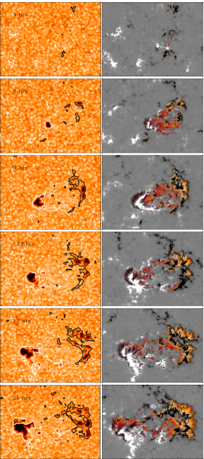
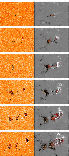
Figure 2: Sequence of the emergence of AR 11105 on the left (first two columns) and AR 11211 on the right. Time increases downwards, showing one image every 4 hours. For each data-set, the first column represents the continuum intensity with the black and white contours showing $B{{}_{LOS}}$ at $\pm$150G. The second column shows $B_{LOS}$ as a gray-scale background saturated between -150 and 150 G (black/white represent negative/positive polarities). Superposed, the headless arrows represent the transverse component of the magnetic field, $B_{T}$, only for pixels in which $B_{T}$ is above the noise level and the inclination is in the $50^{\circ}-130^{\circ}$ range. The black-red-white colour coding indicates values in this range, with red corresponding to purely transverse fields ($90^{\circ}$).

Fig 2 shows the sequence of the emergence for both data-sets. Time increases downwards and only one snapshot every 4 hours is shown. The first two columns correspond to AR 11105 and the other two to AR 11211. For each data-set, the first column represents the continuum intensity in the background with white and black contours showing the line-of-sight magnetic flux density, ${\rm B_{LOS}}$, at $\pm 150\,$G. The second column shows ${\rm B_{LOS}}$ as the grayscale background with superposed (headless) arrows representing the direction of the transverse component of the vector magnetic field, ${\rm B_{T}}$. Arrows are only plotted for pixels whose magnetic field is above the noise level and mostly horizontal with respect to the solar surface (i.e. with inclinations $\theta_{B}$, between $50-130^{\circ}$).

AR 11105 emerges in the Northern Hemisphere on September 1 2010. It grows fast, at large flux rate. Over the first few days of its life it develops many pores that coalesce into larger spots that eventually develop penumbrae. By the time it reaches the West limb, AR 11105 is composed of a large leading sunspot followed by groups of pores and surrounded by strong plage areas. AR 11211, on the other hand, appears in the Southern Hemisphere on May 8 2011. It only develops a few small pores that decay within three days of emerging. After that, its signature disappears completely from the continuum images, only to be seen in the magnetograms. Any magnetic remnant of this region fades away before crossing the West limb.

In this paper we focus on the 24 hours following the first signatures of the emergence. A rough common scenario applies to both ARs: during the first minutes of the emergence process, the only signatures of the AR are a small patch of horizontal fields connecting a magnetic dipole. In the following hours, new bursts of transverse fields bring more flux to the surface. As they rise, the anchoring points of the newly emerged field lines become more and more vertical, and drift and merge with pre-existing flux of the same polarity. The main footpoints of the active regions begin to differentiate themselves from the surrounding flux as they drift apart. After 2-3 hours, the first pores start to appear in the continuum images. The AR carries on growing without interruption, bringing magnetic flux to the surface at a steady rate. One of the differenes between the two ARs is the development of abnormal granulation in the area where the horizontal fields come to the surface. AR 11105 (left columns of figure 2) exhibits this characteristic whenever a new patch of horizontal field appears in the vector-magnetogram - with the granulation becoming brighter, with less contrast and elongated in the direction of the magnetic field. This effect, albeit also present in AR 11211, is not as common or as strong as in the first case (right columns of figure 2), probably because of the weaker nature of the magnetic fields that rise through the surface.

This paper will focus on the magnetic and kinematic properties of naked AR emergence, and the relation between them during these first stages of the emergence.

3.1 Flux history and other magnetic quantities

Figure 3: Flux history for both active regions, NOAA AR 11105 on the left and AR 11211 on the right. The dashed vertical line shows the time at which the first pores appear in the continuum intensity. In the first case, the flux rate is $\sim 4\cdot 10^{19}$ Mx/hr while in the second one, it varies from $1.2$ to $2\cdot 10^{19}$ Mx/hr. Two different linear fits have been applied to the flux evolution of AR 11211, in the first and the second halves of the sequence. This somewhat arbitrary division is marked by the solid vertical line in the right panel of the figure.

Figure 3 shows the flux history for both regions during the first 24 hours of existence. Diamonds represent the negative component and plus signs the positive component of the magnetic flux. In both cases, during the first 15 hours, the positive and negative fluxes are very well balanced. However, over time, the ARs occupy a larger area and a flux imbalance becomes evident. In the case of AR 11211 (right panel), towards the secont half of the sequence, the leading polarity (positive) becomes more compact than the following one. Just because the following polarity is more spread out, some of its signal might lie below the detection threshold of the HMI instrument, leading to a slight imbalance between the measured fluxes. This is not the case for AR 11105 (left), whose positive flux hits the edges of the FOV around hour 16, leading to a loss of flux through the boundaries of the box, and hence to an imbalance in the flux curve.

A linear fit to the flux curves shows that, during the first 12 hours of emergence, the rate of flux brought to the surface by the large active region (AR 11105 at $4\cdot 10^{19}$Mx/hr) triples that of the smaller one (AR 11211). However, the latter increases its flux output to $\sim 2\cdot 10^{19}$Mx/hr during the second half of the day. The solid vertical line at minute 60 marks, approximately, the time when the flux output changes. The vertical dahsed lines in figure 3 show the approximate time at which the first pores are seen in the continuum intensity.

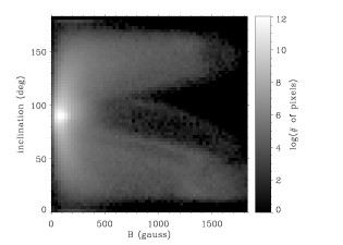
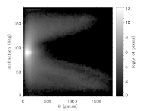
Figure 4: Density scatter plots of the inverted magnetic field inclination vs. the field strength for both ARs during the first 24 hours of emergence. In both cases, the stronger fields are the most vertical ones. The strength of the transverse fields lies in between 150-1000 G for AR 11105 (left) and 150-600 G for AR 11211 (right). Note that everything below 150 G is not reliable.

Figure 4 shows a scatter plot of the magnetic field inclination (with respect to the LOS) vs. the field strength for the combined first 24 hours of emergence. AR 11105 is on the left and AR 11211 on the right. Despite being represented in these figures, transverse fields ($\sim 90^{\circ}$) with strengths below 150 G are the result of the inversion of polarization signals that are pure noise. In fact, the strongest signal in the scatter plots correspond to this “horizontal field effect” of the spectral line inversion, and it has no physical meaning or significance. For both ARs, the strongest fields tend to be mostly vertical. Transverse fields (around 90 degrees of inclination) are comparatively much weaker, ranging between 150-900 G for AR 11105 and 150-400 G for AR 11211.

AR 11105 grows faster and at a higher flux rate than AR 11211. The larger flux rate is not only a consequence of the larger area, but also of the stronger transverse fields that it brings to the surface. Although the spectral line inversion that we use does not account for a magnetic filling factor and hence does not deliver intrinsic field strengths, Kubo et al. (2003) stated that the filling factors in emergence zones are always larger than 80%, which would mean that the strengths that we report here should be close to the intrinsic values. AR 11105 also harbours stronger vertical fields at its footpoints than AR 11211.

3.2 Moving dipolar features

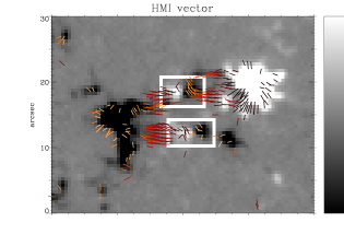
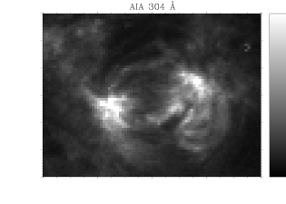
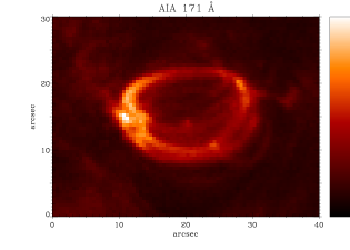
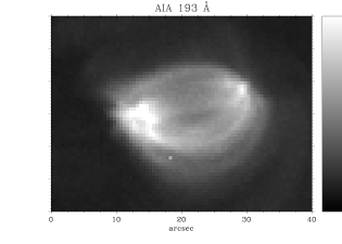
Figure 5: Top left: Detail of the magnetic field configuration around two MDFs (boxed in white) for AR 11211. As usual, the grayscale background represents the longitudinal magnetic flux density (positive/negative in white/black) while the red-ish headless arrows show the transverse component of the magnetic field for inclinations between $50^{\circ}$ and $130^{\circ}$ with respect to the LOS. The polarities of both MDFs are connected to the main footpoints of the AR by horizontal fields, rendering a picture of field lines that serpentine in and out of the solar surface. Top right: Quasi-simultaneous AIA 304 Å image that shows the loop structure in the chromosphere. Bottom: Quasi-simultaneous AIA 171 Å (left) and AIA 193 Å (right) channels showing the structure in the corona.

During the first stages of the emergence process, horizontal magnetic fields connect the footpoints of the AR, which grow fast, drift apart and differentiate themselves as the main dipole where the AR is anchored to the Photosphere. As soon as these footpoints are far enough (5-10”), the flux emergence process starts happening within smaller patches of horizontal fields that do not span the whole distance between the main footpoints. The top left panel of figure 5 shows one snapshot in the emergence of AR 11211. The main footpoints of the AR can be easily seen in the background magnetogram. In between the main polarities, two small dipoles (labelled moving dipolar features, MDFs, by Bernasconi et al., 2002) of opposite polarity to that of the AR, are highlighted by the white boxes. Each of the poles of these MDFs, is connected to one of the main footpoints of the AR by transverse fields (red headless arrows). The color coding of the arrows is such that red indicates a purely transverse field ($\theta=90^{\circ}$), while darker or lighter represent a range of inclinations, between $50^{\circ}\ {\rm and}\ 130^{\circ}$, white being a magnetic field mostly pointing into the solar surface and black pointing outwards (note that this black/white convention is opposite to that of the magnetogram, for clarity purposes). It has to be born in mind that these data have not been disambiguated. However, due to the proximity to disk center, the magnetic field disambiguation would only have a minor effect on the inclination angle and the projected transverse component of $\vec{B}$, rendering a very similar picture to that of Fig. 5. The relatively simple configuration of the AR and the obvious connectivity between each pair of magnetic poles calls for a scenario where the field lines that emerge from the main positive polarity, dip into the photosphere at the locations of the MDFs just to re-emerge again and arch their way over to the negative polarity. MDFs are just a more vertical counterpart of the horizontal field lines represented by the arrows.

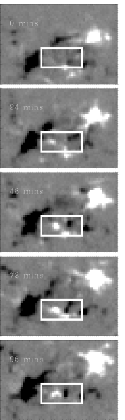
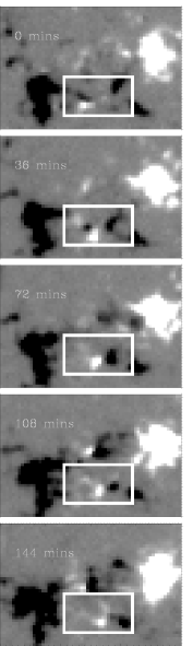
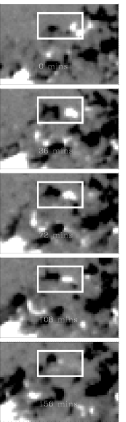
Figure 6: Temporal evolution of three MDFs. The grayscale background in all panels shows the LOS magnetic flux density saturated at $\pm 100$ G. The three columns represent three different events (the left and middle colums correspond to AR 11211 and the right column to AR 11105). Time increases downwards, and the starting time is approximately 3 hrs, 6 hrs and 20 hrs (from left to right) with respect to the first signature of the emergence of the ARs. The white squares highlight isolated MDFs, whose footpoints come closer together in the time span of these sequences. For the sake of showing the final moments of the MDF (when one polarity has been mostly cancelled out by the other), the snapshots are not evenly spread out in time.

Fig. 6 shows the temporal evolution of three individual MDFs, highlighted in the white boxes. The grayscale background shows the LOS magnetic flux density saturated at $\pm 100$ G. Time increases downwards but the snapshots are not necessarily evenly spread out in time. As captured in this figure, the poles of the MDFs often approach each other until they merge, partially cancelling one another and sometimes completely disappearing (the partial cancellation is obvious in the last panels of the middle and the right columns of this figure). This behaviour is in contrast to what Bernasconi et al. (2002) see in their observations, namely that MDFs tend to drift towards one of the main footpoints of the AR and then disappear.

The question of whether a reconnection event takes place below or above the surface, in between the footpoints of the MDF is up to debate. The HMI measurements are blind to the layers below or above the region of sensitivity of its spectral line, hence any conjecture of what happens underneath the surface or in the high the photosphere goes beyond the capability of these observations and the scope of this paper. If the reconnection happened above the photosphere, one would expect to see downflows associated to the cancelling site, where the submerging part of the magnetic loop crosses the surface. If, on the other hand, the reconnection took place below the surface, ascending motions should be present where the arcade finally manages to emerge. The HMI observations at a 12 minute cadence do not provide evidence either way. The spatial and temporal resolution and the uncertainties in the velocity measurements do not offer an answer to this question.

In any case, Cheung et al. (2010) suggest this reconnection as a mechanism to get rid of the mass carried by the rising field lines and Watanabe et al. (2008) even use it to explain the triggering of Ellerman Bombs in the chromosphere.

MDFs are just the signature of emerging field lines that are trapped in the photosphere due to entrained mass that acts as an anchoring weight. Once an MDF cancels out (supposedly after a reconnection of the dipped loop), the magnetic arcade is no longer pinned down to the photosphere at these points and the loop will be free to rise into the corona (while its counterpart submerges into the solar interior). The top right panel of figure 5 shows a near-simultaneous image of the chromosphere taken by the Atmospheric Imaging Assembly (AIA, Lemen et al., 2012) in the 304 Å wavelength. The bottom panels of the same figure show, on the other hand, quasi-simultaneous images of the corona in the AIA 171 and 193 Å channels. While the chromospheric image (at 304 Å) presents loops that are structured a lot like the photospheric field (the lower left side of the image shows shorter loops connecting the lower MDF to the leading footpoint of the AR), the coronal structures span the entire distance between the main footpoints, and are almost oblivious to what happens at the smaller spatial scales seen at photospheric levels. That said, time sequences of AIA 171 and 193 Å, show transient brightenings and small loop-like structures associated to the locations of the MDFs (the simultaneity with the photospheric phenomena cannot be pinned down since the HMI vector data have a much lower cadence). However, most of the time, the overall structure of the coronal images is that of large-scale loops connecting the main footpoints of the AR. These pieces of evidence support a picture in which the emerging horizontal fields pinned down to the photosphere at the MDF locations cannot rise much beyond the chromosphere until the MDF reconnects and the magnetic arcade is released from its photospheric trap.

3.3 Doppler velocities

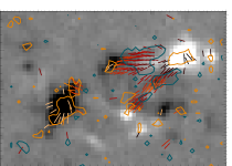
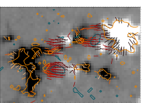
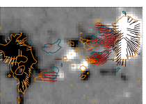
Figure 7: Three non-consecutive snapshots in the evolution of AR 11211. The contours show the Doppler velocities at -200 (blue, upflows) and 200 (orange, downflows) ${\rm ms^{-1}}$ for pixels where the magnetic field strength is above the noise level. The background image shows the longitudinal magnetic flux density saturated at $\pm 100$ gauss (white/black represents positive/negative polarity) and the headless arrows show the mostly transverse component of the field. The FOV of these images is 30 x 20 arcsecs.

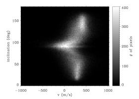
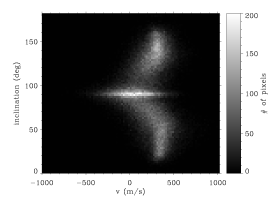
Figure 8: Kinematic aspects for AR 11105 (top) and 11211 (bottom). Left: density scatter plots of the magnetic field inclination versus the Doppler velocity for both active regions. Each plot combines the first 24 hours of emergence and only pixels with magnetic field strength above the noise are considered. An inclination of $90^{\circ}$ corresponds to a magnetic field almost parallel to the solar surface and negative velocities represent upflows. Vertical fields always harbour downflows whilst horizontal fields have a strong correspondence with upflowing material. Right: temporal evolution of the average downflowing velocity at the footpoints of both ARs (defined as where the magnetic field is inclined less than $40^{\circ}$ with respect to the vertical). The velocities are shown separately for the positive and the negative polarities. The vertical dash-dotted line marks, approximately, the time at which the center of the AR passes the central meridian.

One of the main characteristics of the emergence process of ARs is the relation between the plasma flows and the magnetic topology. AR emergence sites are characterized by downflows of up to $2\,{\rm kms^{-1}}$ in the vicinity of rapidly growing pores and by upflows around the main polarity inversion line, where the new magnetic flux is surfacing (see, for instance, Zwaan, 1985; Brants, 1985b).

Figure 7 shows three snapshots in the evolution of AR 11211. Upflows (blue contours) and downflows (orange contours) for the magnetized pixels are plotted over the grayscale background that represents the longitudinal magnetic flux density saturated at $\pm 100$ G). Red arrows show the direction of the transverse component of the magnetic field vector where it is rather inclined with respect to the LOS (forming an angle of less than $40^{\circ}$ from the solar surface). In magnetized areas, there is a strong correlation between the velocity patterns and the magnetic field orientation. Upflows are present wherever the magnetic field has a predominantly transverse nature, whilst downflows are systematically correlated to the more vertical configurations. Although only the velocity contours for magnetized areas are shown in figure 7, it is important to note that the sizes and velocities of the upflow patches do not differ significantly from those of the surrounding quiet Sun at the spatial resolution of the HMI data. Horizontal field patches brought up to the surface span spatial scales of several granules (5 to 10 ″).

The left column of figure 8 shows density scatterplots of the magnetic field inclination versus the Doppler velocity for the first 24 hours of emergence of each of the active regions. An inclination of $90^{\circ}$ corresponds to a magnetic field parallel to the solar surface. It is clear that, during these first stages of the emergence process, the more vertical fields (with inclinations close to 0 and $180^{\circ}$) always harbour downflows, whilst the horizontal component of these fields tends to be accompanied by upflowing material.

Both scatter plots present a slight asymmetry in the Doppler shifts of the AR footpoints. In both cases, the leading polarity ($\theta\sim 180^{\circ}$ for AR 11105 and $\theta\sim 0^{\circ}$ for AR 11211) shows stronger downflows than the following one - this is especially obvious in the case of AR 11105 (top left panel). This is partly due to the proper motions of the footpoints, which drift apart as the AR grows. These proper motions have a line-of-sight component that adds up to the measured Doppler velocity whenever the AR is not at disk center. Our targets are never very far away from disk center for the time span of the observations presented in this paper. However, during the very early stages of emergence (for the first 10-12 hours of the sequence) both ARs are approaching the central meridian from the East side, whilst, for the second half of the sequence, they travel Westwards away from it. One would expect to see a larger LOS component of the proper motions of the footpoints in the second half of the sequence, when the ARs are larger and more developed. On the West side of the meridian, the projection of the proper motion of the footpoints is always in the sense that the leading polarity would seem to be moving away from the observer (redshift) whilst the following polarity would appear to do the opposite (blueshift). Hence, this could explain the Doppler shift asymmetry seen in the scatter plots.

The panels on the right column of Figure 8 show the temporal evolution of the average velocity at the footpoints of both active regions, separated by polarity. The vertical dash-dotted line marks the approximate time when the center of the AR crosses the central meridian. Although AR 11211 (bottom right panel) presents a slight asymmetry of the mean downflows at its footpoints, this is relatively small when compared to the spread in velocity values. Also note that, for a fraction of the time, the following polarity has stronger downflows than the leading one, but the trend switches when the AR is about to cross the meridian. This is likely to be an effect of the footpoint proper motions.

AR 11105, on the other hand, shows a systematic strong asymmetry that does not switch its behavior when crossing from the East to the West side of the meridian. The leading polarity has, on average, $100{\rm ms^{-1}}$ stronger downflows than the following one, suggesting that the imbalance is real and not just a product of transverse motions and projection effects. It is also interesting to note that there is a strong correlation between the flows at both footpoints (see how the solid and dashed lines of the top right panel of figure 8 follow each other’s trend). This supports the idea of a net flow going from the following to the leading polarity (the flow becomes stronger or weaker at both footpoints in synchrony).

In both ARs, downflows are present in the entire area of the pores, being stronger at the edges. MDF’s, albeit usually less vertical than the main footpoints of the AR, also harbour consistent downflows during their short lifetimes.

3.4 Continuum intensity

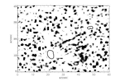
Figure 9: Negative snapshot of the continuum intensity of AR 11105, saturated below $1.013\cdot{\rm I_{CONT}}$ (white). Black contours mark the locations of the pores over the grayscale background, where only the brighter granules stand out. The granulation pattern in between the footpoints of the AR often shows fibrilar structures, lower contrasts and higher-than-average intenisties.

The regions of emergence of the top of the magnetic arcades are characterized by horizontal fields and upflowing velocities. The granulation in these areas is often elongated in the direction that connects the main footpoints of the AR (see, for instance Schlichenmaier et al., 2010; Cheung et al., 2010; Stein et al., 2011b). Small-scale short-lived dark features in the Photosphere and the Chromosphere, often followed by brightenings, accompany the emergence. These events are thought to be the signature of arch filament systems of the scale of several granules, rising up from the photosphere to the chromosphere (Vargas Domínguez et al., 2012).

The spatial resolution of the HMI data imposes some constraints on the analysis of granular-scale events. Nevertheless, the data allow us to witness some of the characteristical properties of granulation at the emergence site (in between the main footpoints of the AR). Elongated bright features are a common sighting in these areas. Figure 9 enhances these occurrences by masking out anything that is darker than 1.013 times the average continuum intensity of the surrounding quiet Sun, highlighting the brighter granules only (note that it is a negative image, so a lighter shade of gray represents a lower continuum intensity). The black contours show the locations of the pores. Elongated bright features can be seen in between the AR footpoints. They are always are co-spatial with patches of horizontal magnetic field and parallel to the direction of the field lines (note that these are not always necessarily aligned with the general orientation of the active region, though). Sometimes, short-lived (30 minutes or less) dark filamentary structures also pop up in these areas, often delineating the brighter elongated ones.

Emergence sites are also characterized by other granulation peculiarities. The average continuum intensity in the area in between the footpoints of the AR exceeds by 0.3-2% that of the quiet Sun in both of our datasets. The strongest excesses are co-temporal and co-spatial with the occurrance of the strongest patches of horizontal fields. Also, despite the brightenings and darkenings taking place, granulation has a systematically lower rms contrast in the emergence site than in the quieter places in the vicinity of the AR. This excess intensity of the granulation in the emergence zone could be a consequence of the larger radiative losses of the hotter plasma that is dragged up to the surface by the buoyant fields. It could also be due to the pressure balance requirement in and around the emerging site. The weak horizontal fields (200-500 G) create a magnetic pressure that has to be compensated by a lower gas pressure. This leads to a less dense environment that is consequently more transparent so the spectral lines will form at deeper (hotter) layers.

4 Discussion

This paper focuses on the “naked” emergence of active regions from their first imprints on the solar surface. With this purpose in mind, we follow the first 24 hours of existence of two relatively-isolated active regions using sequences of photospheric vector magnetic fields and Doppler velocities obtained with the Helioseismic and Magnetic Imager on board SDO.

AR 11105 grows faster and at 3 times the flux rate of AR 11211. It brings intrinsically stronger transverse fields to the surface (up to 1000 G as opposed to 400 G) and harbours stronger vertical fields at its footpoints. It also presents a systematic asymmetry in the downflowing plasma at its footpoints, with the leading polarity having, on average, $100{\rm ms^{-1}}$ faster downflows than the following one. This characteristic together with the strong correlation in the strength of the flows at both footpoints, suggests the existence of a net flow from the following to the leading polarity, in agreement with the findings by Cauzzi et al. (1996) and in disagreement with certain models of flux emergence (Fan et al., 1993). This flow asymmetry is not clear in the smaller AR.

Qualitatively, however, both ARs display a similar behaviour during emergence. The process of the “naked” emergence of an AR is simplified in the cartoon of figure 10. The very first signature of an AR on the surface is a relatively simple dipole connected by horizontal fields. Small (5 - 15″) bursts of transverse field patches flanked by more vertical footpoints keep bringing new flux to the surface. As the vertical magnetic features coalesce, the AR starts growing appreciably and its main footpoints differentiate themselves and drift apart. Systematic downflows begin to dominate at the places where the field is anchored to the photosphere. Once the AR reaches a certain size, the patches of horizontal field do not span the entire distance between the main footpoints anymore. Instead, they connect via an intermediate layer of MDFs (dipoles of opposite polarity to that of the AR) that appears in between the two polarities. Upflows characterize the patches of transverse field while plasma drains back down into the photosphere through all of the places where the field is pinned down to the surface. Brighter granulation, elongated in the direction of the magnetic field, often accompanies the horizontal patches. This characteristic is more evident the stronger the magnetic flux is. When the AR is big enough, several layers of MDFs coexist in the emergence zone. The magnetic field contributing to the global emergence serpentines into and out of the surface from the main positive polarity to the negative one, process that is commonly referred to in the literature as resistive emergence (e.g. Pariat et al., 2004, 2009). In this scenario, the MDFs are just the drainage points of the plasma carried by the upwelling field lines. The poles of MDFs tend to approach each other and cancel out, presumably reconnecting somewhere close to the surface (below or above) and releasing the field lines that are now free to continue rising up into the corona. This is consistent with the scenario described by Cheung et al. (2010), where the cancelling MDFs are the visual signature of the reconnection of field lines and the discharge of mass from the rising magnetic structure.

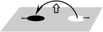
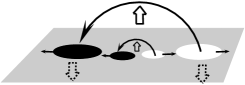
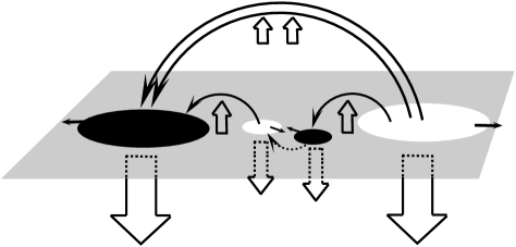
Figure 10: Sequence of the naked emergence of an AR. The first photospheric signature is a small dipole connected by horizontal fields. Patches of transverse fields continue to emerge with their corresponding footpoints, which drift and merge with the pre-existing ones. When the AR is large enough, the magnetic arcade is not able to lift the weight of the plasma that it carries and remains trapped to the photosphere at the locations of the MDFs. The poles of the MDFs approach one another and cancel out, liberating the field lines and letting the arcade rise into the corona.

5 Acknowledgments

The National Center for Atmospheric Research is sponsored by the National Science Foundation. This manuscript was mostly written while RC was a visiting scientist at the Kiepenheuer-Insitut für Sonnenphysik (Freiburg, Germany). RC wishes to thank Rolf Schlichenmaier, Juan Borrero, Wolfgang Schmidt, Valentín Martínez Pillet and Alfred de Wijn for insightful comments on this piece of research.

References

- (1)
- Bernasconi et al. (2002) Bernasconi, P. N., Rust, D. M., Georgoulis, M. K., & Labonte, B. J. 2002, Sol. Phys., 209, 119
- Borrero et al. (2011) Borrero, J. M., Tomczyk, S., Kubo, M., Socas-Navarro, H., Schou, J., Couvidat, S., & Bogart, R. 2011, Sol. Phys., 273, 267
- Brants (1985a) Brants, J. J. 1985a, Sol. Phys., 95, 15
- Brants (1985b) —. 1985b, Sol. Phys., 98, 197
- Brants & Steenbeek (1985) Brants, J. J. & Steenbeek, J. C. M. 1985, Sol. Phys., 96, 229
- Cauzzi et al. (1996) Cauzzi, G., Canfield, R. C., & Fisher, G. H. 1996, ApJ, 456, 850
- Cheung et al. (2010) Cheung, M. C. M., Rempel, M., Title, A. M., & Schüssler, M. 2010, ApJ, 720, 233
- Fan (2009) Fan, Y. 2009, Living Reviews in Solar Physics, 6, 4
- Fan et al. (1993) Fan, Y., Fisher, G. H., & Deluca, E. E. 1993, ApJ, 405, 390
- Hale (1908) Hale, G. E. 1908, ApJ, 28, 315
- Kubo et al. (2003) Kubo, M., Shimizu, T., & Lites, B. W. 2003, ApJ, 595, 465
- Lemen et al. (2012) Lemen, J. R., Title, A. M., Akin, D. J., Boerner, P. F., Chou, C., Drake, J. F., Duncan, D. W., Edwards, C. G., Friedlaender, F. M., Heyman, G. F., Hurlburt, N. E., Katz, N. L., Kushner, G. D., Levay, M., Lindgren, R. W., Mathur, D. P., McFeaters, E. L., Mitchell, S., Rehse, R. A., Schrijver, C. J., Springer, L. A., Stern, R. A., Tarbell, T. D., Wuelser, J.-P., Wolfson, C. J., Yanari, C., Bookbinder, J. A., Cheimets, P. N., Caldwell, D., Deluca, E. E., Gates, R., Golub, L., Park, S., Podgorski, W. A., Bush, R. I., Scherrer, P. H., Gummin, M. A., Smith, P., Auker, G., Jerram, P., Pool, P., Soufli, R., Windt, D. L., Beardsley, S., Clapp, M., Lang, J., & Waltham, N. 2012, Sol. Phys., 275, 17
- Lites et al. (2010) Lites, B. W., Kubo, M., Berger, T., Frank, Z., Shine, R., Tarbell, T., Title, A., Okamoto, T. J., & Otsuji, K. 2010, ApJ, 718, 474
- Lites et al. (1998) Lites, B. W., Skumanich, A., & Martinez Pillet, V. 1998, A&A, 333, 1053
- MacTaggart (2011) MacTaggart, D. 2011, A&A, 531, A108
- Moreno-Insertis (1997) Moreno-Insertis, F. 1997, Mem. Soc. Astron. Italiana, 68, 429
- Norton et al. (2006) Norton, A. A., Graham, J. P., Ulrich, R. K., Schou, J., Tomczyk, S., Liu, Y., Lites, B. W., López Ariste, A., Bush, R. I., Socas-Navarro, H., & Scherrer, P. H. 2006, Sol. Phys., 239, 69
- Pariat et al. (2004) Pariat, E., Aulanier, G., Schmieder, B., Georgoulis, M. K., Rust, D. M., & Bernasconi, P. N. 2004, ApJ, 614, 1099
- Pariat et al. (2009) Pariat, E., Masson, S., & Aulanier, G. 2009, ApJ, 701, 1911
- Pesnell et al. (2012) Pesnell, W. D., Thompson, B. J., & Chamberlin, P. C. 2012, Sol. Phys., 275, 3
- Sánchez Almeida & Martínez González (2011) Sánchez Almeida, J. & Martínez González, M. 2011, in Astronomical Society of the Pacific Conference Series, Vol. 437, Solar Polarization 6, ed. J. R. Kuhn, D. M. Harrington, H. Lin, S. V. Berdyugina, J. Trujillo-Bueno, S. L. Keil, & T. Rimmele, 451
- Schlichenmaier et al. (2010) Schlichenmaier, R., Rezaei, R., Bello González, N., & Waldmann, T. A. 2010, A&A, 512, L1
- Schou et al. (2012) Schou, J., Scherrer, P. H., Bush, R. I., Wachter, R., Couvidat, S., Rabello-Soares, M. C., Bogart, R. S., Hoeksema, J. T., Liu, Y., Duvall, T. L., Akin, D. J., Allard, B. A., Miles, J. W., Rairden, R., Shine, R. A., Tarbell, T. D., Title, A. M., Wolfson, C. J., Elmore, D. F., Norton, A. A., & Tomczyk, S. 2012, Sol. Phys., 275, 229
- Sigwarth et al. (1998) Sigwarth, M., Schmidt, W., & Schuessler, M. 1998, A&A, 339, L53
- Stein et al. (2011a) Stein, R. F., Lagerfjärd, A., Nordlund, Å., & Georgobiani, D. 2011a, Sol. Phys., 268, 271
- Stein et al. (2011b) —. 2011b, Sol. Phys., 268, 271
- Strous (1994) Strous, L. H. 1994, PhD thesis, PhD Thesis, Utrecht University, (1994)
- Strous & Zwaan (1999) Strous, L. H. & Zwaan, C. 1999, ApJ, 527, 435
- van Ballegooijen (2008) van Ballegooijen, A. A. 2008, in Astronomical Society of the Pacific Conference Series, Vol. 383, Subsurface and Atmospheric Influences on Solar Activity, ed. R. Howe, R. W. Komm, K. S. Balasubramaniam, & G. J. D. Petrie, 191
- Vargas Domínguez et al. (2012) Vargas Domínguez, S., van Driel-Gesztelyi, L., & Bellot Rubio, L. R. 2012, Sol. Phys., 278, 99
- Walton et al. (1994) Walton, S. R., Corbin, K. H., & Chapman, G. A. 1994, in Astronomical Society of the Pacific Conference Series, Vol. 68, Solar Active Region Evolution: Comparing Models with Observations, ed. K. S. Balasubramaniam & G. W. Simon, 75
- Watanabe et al. (2008) Watanabe, H., Kitai, R., Okamoto, K., Nishida, K., Kiyohara, J., Ueno, S., Hagino, M., Ishii, T. T., & Shibata, K. 2008, ApJ, 684, 736
- Westendorp Plaza et al. (1998) Westendorp Plaza, C., del Toro Iniesta, J. C., Ruiz Cobo, B., Martinez Pillet, V., Lites, B. W., & Skumanich, A. 1998, ApJ, 494, 453
- Zhang et al. (2012) Zhang, Y., Kitai, R., & Takizawa, K. 2012, ApJ, 751, 85
- Zuccarello et al. (2008) Zuccarello, F., Battiato, V., Contarino, L., Guglielmino, S., Romano, P., & Spadaro, D. 2008, A&A, 488, 1117
- Zwaan (1985) Zwaan, C. 1985, Sol. Phys., 100, 397